分类: 强化学习作业代写

机器学习代写|强化学习project代写reinforence learning代考|Actor-Critic Hypothesis

如果你也在 怎样代写强化学习reinforence learning这个学科遇到相关的难题,请随时右上角联系我们的24/7代写客服。

强化学习是一种基于奖励期望行为和/或惩罚不期望行为的机器学习训练方法。一般来说,强化学习代理能够感知和解释其环境,采取行动并通过试验和错误学习。

statistics-lab™ 为您的留学生涯保驾护航 在代写强化学习reinforence learning方面已经树立了自己的口碑, 保证靠谱, 高质且原创的统计Statistics代写服务。我们的专家在代写强化学习reinforence learning代写方面经验极为丰富,各种代写强化学习reinforence learning相关的作业也就用不着说。

我们提供的强化学习reinforence learning及其相关学科的代写,服务范围广, 其中包括但不限于:

  • Statistical Inference 统计推断
  • Statistical Computing 统计计算
  • Advanced Probability Theory 高等概率论
  • Advanced Mathematical Statistics 高等数理统计学
  • (Generalized) Linear Models 广义线性模型
  • Statistical Machine Learning 统计机器学习
  • Longitudinal Data Analysis 纵向数据分析
  • Foundations of Data Science 数据科学基础
on-policy vs. off-policy actor-critic : r/reinforcementlearning
机器学习代写|强化学习project代写reinforence learning代考|Actor-Critic Hypothesis

机器学习代写|强化学习project代写reinforence learning代考|Actor-Critic Hypothesis

Houk, Adams and Barto attempted to solve the credit assignment problem in animals by linking activity of dopamine neurons in the basal ganglia to an actor-critic model [8]. There is evidence that links an actor to habitual behavior (stimulus response or S-R associations) of mammals with action selection mechanisms in the dorsolateral striatum located in the basal ganglia [14].

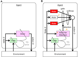
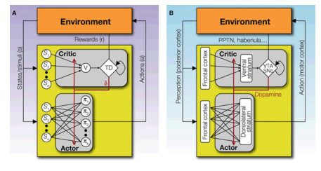
In his review on reinforcement learning and the neural basis of conditioning, Tiago V. Maia states that in order for an area to be taken seriously as the critic, it needs to fulfill three requirements. The area should show neuronal activity during the expectation of reward. The area should also show activation during an unexpected reward or a reward-predicting stimulus but not in the period between predictor and the reward itself. The third requirement is that the area should project to and from neurons in the dopamine system because they represent prediction errors as discussed in the section above [12]. The ventral striatum fulfills all three criteria. It has been shown that the expectation of external events with behavioral significance is related to activity in the ventral striatum [19]. This area also sends dopaminergic projections to and receives from all regions in the striatum including what is hypothesized to be the actor [10]. The orbitofrontal cortex and the amygdala are two other structures in the brain that also fulfill these criteria [17]. The two areas are both anatomically and functionally closely related to the ventral striatum [1]. Fig. I shows a diagram that depicts how the structure of a neural actor-critic might look like. The actor in the dorsolateral striatum receives its input from the posterior regions (somatosensory and visual cortices) and sends action decisions back to the environment through signals to the motor cortex. The critic in the ventral striatum computes the prediction error and returns it to the actor through dopamine projections to the dorsal striatum.

机器学习代写|强化学习project代写reinforence learning代考|Multiple Critics Hypothesis

As was mentioned in the previous subsection, the amygdala and the orbitofrontal cortex are also correlated with learning and have dopamine receptors/projections from and to the dorsal striatum. The former shows activation patterns during emotional learning [13] and the latter during associative learning [6]. This raises the question of whether there can be multiple critics with different criteria interacting with each other. The main function of each structure could represent a unique criterion that perhaps projects its value to the other areas. If this hypothesis is valid, then we might see excitatory or inhibitory dopamine receptors being activated by presynaptic neurons in the amygdala during learning while different emotions that trigger activation in the amgydala are induced. Furthermore, it would be interesting to investigate the role of different dopamine transmitter sub-types and receptors that might play different learning roles in these structures.

机器学习代写|强化学习project代写reinforence learning代考|Limitations

The main difficulty with neuroscience research is our limited understanding of how biochemical reactions in the brain can represent and process information. Studies on humans are conducted mostly with fMRI and EEG (electroencephalography). fMRI achieves relatively high spatial resolution with one voxel representing a few million neurons and tens of billions of synapses [9]. However, fMRI has low temporal resolution producing images after 1 second of the event. This is not desirable when we consider that prediction errors are time-based. EEG measures electrophysiological activity by placing non-invasive electrodes on the scull. The electrodes achieve a high temporal resolution in the range of milliseconds but with a very low spatial resolution. This is due to volume conduction and other distortions which can even affect the validity of the temporal resolution [3].

Transferring concepts of reinforcement learning between psychology, neuroscience and computer science has resulted in mutual progress. The early development of classical conditioning in behavioral psychology eventually resulted in TD learning and an actor-critic paradigm is now being hypothesized to function in the brain. We believe that despite current limitations in measurement technologies, future research which integrates integrates reinforcement learning in psychology, neuroscience, and computer science can bring novel theories to the three fields.

Towered Actor Critic For Handling Multiple Action Types In Reinforcement  Learning For Drug Discovery
机器学习代写|强化学习project代写reinforence learning代考|Actor-Critic Hypothesis

强化学习代写

机器学习代写|强化学习project代写reinforence learning代考|Actor-Critic Hypothesis

Houk、Adams 和 Barto 试图通过将基底神经节中多巴胺神经元的活动与演员-评论模型联系起来来解决动物的信用分配问题 [8]。有证据表明,行为者与哺乳动物的习惯行为(刺激反应或 SR 关联)与位于基底神经节的背外侧纹状体中的行为选择机制有关 [14]。

在他对强化学习和条件反射的神经基础的评论中,Tiago V. Maia 指出,为了让一个领域被认真对待,它需要满足三个要求。该区域应在期望奖励期间显示神经元活动。该区域还应该在意外奖励或奖励预测刺激期间显示激活,但不是在预测变量和奖励本身之间的时期内。第三个要求是该区域应该投射到多巴胺系统中的神经元和从多巴胺系统中的神经元投射,因为它们代表了上面部分中讨论的预测误差[12]。腹侧纹状体满足所有三个标准。已经表明,对具有行为意义的外部事件的预期与腹侧纹状体的活动有关 [19]。该区域还向纹状体的所有区域发送和接收多巴胺能投射,包括被假设为演员的区域 [10]。眶额皮质和杏仁核是大脑中另外两个也符合这些标准的结构 [17]。这两个区域在解剖学和功能上都与腹侧纹状体密切相关 [1]。图 I 显示了一个图表,描述了神经演员-评论家的结构可能是什么样子。背外侧纹状体中的参与者接收来自后部区域(躯体感觉和视觉皮层)的输入,并通过运动皮层的信号将动作决策发送回环境。腹侧纹状体中的批评者计算预测误差并通过多巴胺对背侧纹状体的投射将其返回给演员。

机器学习代写|强化学习project代写reinforence learning代考|Multiple Critics Hypothesis

如前一小节所述,杏仁核和眶额叶皮层也与学习相关,并且具有来自和到背侧纹状体的多巴胺受体/投射。前者显示情绪学习期间的激活模式[13],后者显示关联学习期间的激活模式[6]。这就提出了一个问题,即是否可以有多个具有不同标准的评论家相互影响。每个结构的主要功能可以代表一个独特的标准,可能会将其价值投射到其他领域。如果这个假设是有效的,那么我们可能会看到兴奋性或抑制性多巴胺受体在学习过程中被杏仁核中的突触前神经元激活,而引发杏仁核激活的不同情绪被诱导。此外,

机器学习代写|强化学习project代写reinforence learning代考|Limitations

神经科学研究的主要困难是我们对大脑中的生化反应如何代表和处理信息的理解有限。对人类的研究主要使用 fMRI 和 EEG(脑电图)进行。fMRI 实现了相对较高的空间分辨率,一个体素代表数百万个神经元和数百亿个突触 [9]。然而,fMRI 在事件发生 1 秒后生成图像的时间分辨率较低。当我们认为预测误差是基于时间的时,这是不可取的。EEG 通过在双桨上放置非侵入性电极来测量电生理活动。电极实现了毫秒范围内的高时间分辨率,但空间分辨率非常低。

在心理学、神经科学和计算机科学之间转移强化学习的概念已经导致相互进步。行为心理学中经典条件反射的早期发展最终导致了 TD 学习,现在假设演员-批评范式在大脑中发挥作用。我们相信,尽管目前测量技术存在局限性,但未来将强化学习与心理学、神经科学和计算机科学相结合的研究可以为这三个领域带来新的理论。

机器学习代写|强化学习project代写reinforence learning代考 请认准statistics-lab™

统计代写请认准statistics-lab™. statistics-lab™为您的留学生涯保驾护航。

金融工程代写

金融工程是使用数学技术来解决金融问题。金融工程使用计算机科学、统计学、经济学和应用数学领域的工具和知识来解决当前的金融问题,以及设计新的和创新的金融产品。

非参数统计代写

非参数统计指的是一种统计方法,其中不假设数据来自于由少数参数决定的规定模型;这种模型的例子包括正态分布模型和线性回归模型。

广义线性模型代考

广义线性模型(GLM)归属统计学领域,是一种应用灵活的线性回归模型。该模型允许因变量的偏差分布有除了正态分布之外的其它分布。

术语 广义线性模型(GLM)通常是指给定连续和/或分类预测因素的连续响应变量的常规线性回归模型。它包括多元线性回归,以及方差分析和方差分析(仅含固定效应)。

有限元方法代写

有限元方法(FEM)是一种流行的方法,用于数值解决工程和数学建模中出现的微分方程。典型的问题领域包括结构分析、传热、流体流动、质量运输和电磁势等传统领域。

有限元是一种通用的数值方法,用于解决两个或三个空间变量的偏微分方程(即一些边界值问题)。为了解决一个问题,有限元将一个大系统细分为更小、更简单的部分,称为有限元。这是通过在空间维度上的特定空间离散化来实现的,它是通过构建对象的网格来实现的:用于求解的数值域,它有有限数量的点。边界值问题的有限元方法表述最终导致一个代数方程组。该方法在域上对未知函数进行逼近。[1] 然后将模拟这些有限元的简单方程组合成一个更大的方程系统,以模拟整个问题。然后,有限元通过变化微积分使相关的误差函数最小化来逼近一个解决方案。

tatistics-lab作为专业的留学生服务机构,多年来已为美国、英国、加拿大、澳洲等留学热门地的学生提供专业的学术服务,包括但不限于Essay代写,Assignment代写,Dissertation代写,Report代写,小组作业代写,Proposal代写,Paper代写,Presentation代写,计算机作业代写,论文修改和润色,网课代做,exam代考等等。写作范围涵盖高中,本科,研究生等海外留学全阶段,辐射金融,经济学,会计学,审计学,管理学等全球99%专业科目。写作团队既有专业英语母语作者,也有海外名校硕博留学生,每位写作老师都拥有过硬的语言能力,专业的学科背景和学术写作经验。我们承诺100%原创,100%专业,100%准时,100%满意。

随机分析代写


随机微积分是数学的一个分支,对随机过程进行操作。它允许为随机过程的积分定义一个关于随机过程的一致的积分理论。这个领域是由日本数学家伊藤清在第二次世界大战期间创建并开始的。

时间序列分析代写

随机过程,是依赖于参数的一组随机变量的全体,参数通常是时间。 随机变量是随机现象的数量表现,其时间序列是一组按照时间发生先后顺序进行排列的数据点序列。通常一组时间序列的时间间隔为一恒定值(如1秒,5分钟,12小时,7天,1年),因此时间序列可以作为离散时间数据进行分析处理。研究时间序列数据的意义在于现实中,往往需要研究某个事物其随时间发展变化的规律。这就需要通过研究该事物过去发展的历史记录,以得到其自身发展的规律。

回归分析代写

多元回归分析渐进(Multiple Regression Analysis Asymptotics)属于计量经济学领域,主要是一种数学上的统计分析方法,可以分析复杂情况下各影响因素的数学关系,在自然科学、社会和经济学等多个领域内应用广泛。

MATLAB代写

MATLAB 是一种用于技术计算的高性能语言。它将计算、可视化和编程集成在一个易于使用的环境中,其中问题和解决方案以熟悉的数学符号表示。典型用途包括:数学和计算算法开发建模、仿真和原型制作数据分析、探索和可视化科学和工程图形应用程序开发,包括图形用户界面构建MATLAB 是一个交互式系统,其基本数据元素是一个不需要维度的数组。这使您可以解决许多技术计算问题,尤其是那些具有矩阵和向量公式的问题,而只需用 C 或 Fortran 等标量非交互式语言编写程序所需的时间的一小部分。MATLAB 名称代表矩阵实验室。MATLAB 最初的编写目的是提供对由 LINPACK 和 EISPACK 项目开发的矩阵软件的轻松访问,这两个项目共同代表了矩阵计算软件的最新技术。MATLAB 经过多年的发展,得到了许多用户的投入。在大学环境中,它是数学、工程和科学入门和高级课程的标准教学工具。在工业领域,MATLAB 是高效研究、开发和分析的首选工具。MATLAB 具有一系列称为工具箱的特定于应用程序的解决方案。对于大多数 MATLAB 用户来说非常重要,工具箱允许您学习应用专业技术。工具箱是 MATLAB 函数(M 文件)的综合集合,可扩展 MATLAB 环境以解决特定类别的问题。可用工具箱的领域包括信号处理、控制系统、神经网络、模糊逻辑、小波、仿真等。

R语言代写问卷设计与分析代写
PYTHON代写回归分析与线性模型代写
MATLAB代写方差分析与试验设计代写
STATA代写机器学习/统计学习代写
SPSS代写计量经济学代写
EVIEWS代写时间序列分析代写
EXCEL代写深度学习代写
SQL代写各种数据建模与可视化代写

机器学习代写|强化学习project代写reinforence learning代考| Instrumental Conditioning

如果你也在 怎样代写强化学习reinforence learning这个学科遇到相关的难题,请随时右上角联系我们的24/7代写客服。

强化学习是一种基于奖励期望行为和/或惩罚不期望行为的机器学习训练方法。一般来说,强化学习代理能够感知和解释其环境,采取行动并通过试验和错误学习。

statistics-lab™ 为您的留学生涯保驾护航 在代写强化学习reinforence learning方面已经树立了自己的口碑, 保证靠谱, 高质且原创的统计Statistics代写服务。我们的专家在代写强化学习reinforence learning代写方面经验极为丰富,各种代写强化学习reinforence learning相关的作业也就用不着说。

我们提供的强化学习reinforence learning及其相关学科的代写,服务范围广, 其中包括但不限于:

  • Statistical Inference 统计推断
  • Statistical Computing 统计计算
  • Advanced Probability Theory 高等概率论
  • Advanced Mathematical Statistics 高等数理统计学
  • (Generalized) Linear Models 广义线性模型
  • Statistical Machine Learning 统计机器学习
  • Longitudinal Data Analysis 纵向数据分析
  • Foundations of Data Science 数据科学基础
机器学习代写|强化学习project代写reinforence learning代考| Instrumental Conditioning

机器学习代写|强化学习project代写reinforence learning代考|Operant Conditioning

In instrumental conditioning, animals learn to modify their behavior in order to enforce a reward or to repress a punishment. The difference to classical conditioning is therefore that the animal does not receive the reward if he does not a perform desired action. As mentioned above, Thorndike already provided early evidence for this behavior in his law of effect. In some of the experiments, cats were put in puzzle boxes and they had to escape in order to receive a reward (like food). He noted that the cats initially tried actions that appeared random but gradually started to stamp out behavior which was not successful and stamp in rewarding behavior. As one could imagine, the cat became faster after a while. This showed that the cats were learning by trial and error and Thorndike called this the “law of effect”. The idea of the law of effect corresponds to learning algorithms that select among different alternatives and that actions on specific states are associated with a reward or even a right step to the expected future reward. Influenced by Thorndike’s research, Hull and Skinner argued that behavior is selected on the basis of the consequences they produce and coined the term operant conditioning. For his experiments, Skinner invented what is now called Skinner’s box in which he put pigeons that can press a lever in order to get a reward. Skinner further popularized what he called the process of shaping. Shaping occurs when the trainer rewards the agent with any taken action that has a slight resemblance to the desired behavior and this process converged to the correct result when applied to pigeons [21]. This process can be directly mapped to reward shaping in reinforcement learning.

机器学习代写|强化学习project代写reinforence learning代考|Neural View

Neuroscience is the field that is concerned with studying the structure and function of the central nervous system including the brain. Neurons are the basic building blocks of brains and, unlike other cells, are densely interconnected. On average each neuron has 7000 synaptic connections and the cerebral cortex alone (the folded outer layer of the brain) is estimated to have $1.5 \times 10^{14}$ synapses [5]. Synaptic connections can be of a chemical or an electrical nature. We concentrate on the former because they are a basis for synaptic plasticity which is correlated with learning [7]. According to the Hebbian theory, repeated stimulation of the postsynaptic neurons increases or decreases the synaptic efficacy. Chemical communication occurs through the synapses by secreting neurotransmitters from the presynaptic cell to receptors on the postsynaptic cell through the synaptic cleft. Fig. 2 shows an illustration of such a chemical synapse. The effect of these neurotransmitters on the postsynaptic neurons can be of an excitatory or an inhibitory nature. Dopamine is perhaps the most famous neurotransmitter. Dopamine plays a role in multiple brain areas and is correlated with different brain functions including learning and will be discussed further in the subsections below. A key feature that makes dopamine a promising candidate to be involved with learning is that the dopamine system is a neuromodulator. Neuromodulators are not as restricted as excitatory or inhibitory neurotransmitters and can reach distant regions in the CNS and affect large numbers of neurons simultaneously.

机器学习代写|强化学习project代写reinforence learning代考|Reward Prediction Error Hypothesis

Work by Schultz et al. and others have shown that there is a strong similarity between the phasic activation of midbrain dopamine neurons and the prediction error $\delta[20]$. They showed that when an animal receives an unpredicted reward, dopamine neuron activity increases substantially. After the conditioning phase, the neuronal activity relocates to the moment when the $\mathrm{CS}$ is presented and not of the reward itself. If the $\mathrm{CS}$ is presented but with omitting the reward afterwards, a decrease of the activity below the baseline is observed approximately at the moment when the reward was presented during conditioning. These observations are consistent with the concept of prediction error. Findings from functional Magnetic Resonance Imaging (fMRI) have shown activation correlated with prediction errors in the striatum and the orbitofrontal cortex [2]. The presence or absence of activity related to prediction errors in the striatum distinguishes participants who learn to perform optimally from those who do not [18].

机器学习代写|强化学习project代写reinforence learning代考| Instrumental Conditioning

强化学习代写

机器学习代写|强化学习project代写reinforence learning代考|Operant Conditioning

在工具性条件反射中,动物学会改变自己的行为以强制奖励或抑制惩罚。因此,与经典条件反射的不同之处在于,如果动物没有执行所需的动作,则不会获得奖励。如上所述,桑代克已经在他的效力定律中为这种行为提供了早期证据。在一些实验中,猫被放在拼图盒中,它们必须逃跑才能获得奖励(比如食物)。他指出,猫最初会尝试看似随机的行为,但逐渐开始消除不成功的行为并刻意奖励行为。可以想象,过了一会儿,猫变得更快了。这表明猫是通过反复试验来学习的,桑代克称之为“效果法则”。效应定律的概念对应于在不同备选方案中进行选择的学习算法,并且对特定状态的动作与奖励相关联,甚至与预期未来奖励的正确步骤相关联。受桑代克研究的影响,赫尔和斯金纳认为,行为是根据它们产生的后果来选择的,并创造了操作性条件反射一词。在他的实验中,斯金纳发明了现在被称为斯金纳的盒子,他在里面放了可以按下杠杆以获得奖励的鸽子。斯金纳进一步普及了他所谓的塑造过程。当训练员用与预期行为略有相似之处的任何行动奖励代理时,就会发生塑造,并且当应用于鸽子时,这个过程会收敛到正确的结果[21]。

机器学习代写|强化学习project代写reinforence learning代考|Neural View

神经科学是研究包括大脑在内的中枢神经系统的结构和功能的领域。神经元是大脑的基本组成部分,与其他细胞不同,它们紧密相连。平均每个神经元有 7000 个突触连接,仅大脑皮层(大脑的折叠外层)估计有1.5×10¹⁴突触[5]。突触连接可以是化学或电气性质的。我们专注于前者,因为它们是与学习相关的突触可塑性的基础[7]。根据赫布理论,对突触后神经元的反复刺激会增加或减少突触的功效。通过突触间隙将神经递质从突触前细胞分泌到突触后细胞上的受体,从而通过突触发生化学通讯。图 2 显示了这种化学突触的示意图。这些神经递质对突触后神经元的影响可以是兴奋性或抑制性的。多巴胺可能是最著名的神经递质。多巴胺在多个大脑区域中发挥作用,并与包括学习在内的不同大脑功能相关,将在下面的小节中进一步讨论。使多巴胺成为参与学习的有希望的候选者的一个关键特征是多巴胺系统是一种神经调节剂。神经调节剂不像兴奋性或抑制性神经递质那样受到限制,可以到达中枢神经系统的较远区域并同时影响大量神经元。

机器学习代写|强化学习project代写reinforence learning代考|Reward Prediction Error Hypothesis

舒尔茨等人的工作。和其他人已经表明,中脑多巴胺神经元的阶段性激活与预测误差之间存在很强的相似性d[20]. 他们表明,当动物获得意想不到的奖励时,多巴胺神经元的活动会大幅增加。在调节阶段之后,神经元活动重新定位到C小号是呈现出来的,而不是奖励本身。如果C小号被呈现但随后省略了奖励,大约在调节期间呈现奖励的那一刻观察到低于基线的活动减少。这些观察结果与预测误差的概念是一致的。功能性磁共振成像 (fMRI) 的研究结果表明,激活与纹状体和眶额皮质的预测误差相关 [2]。纹状体中是否存在与预测误差相关的活动将学习最佳表现的参与者与不学习的参与者区分开来[18]。

机器学习代写|强化学习project代写reinforence learning代考 请认准statistics-lab™

统计代写请认准statistics-lab™. statistics-lab™为您的留学生涯保驾护航。

金融工程代写

金融工程是使用数学技术来解决金融问题。金融工程使用计算机科学、统计学、经济学和应用数学领域的工具和知识来解决当前的金融问题,以及设计新的和创新的金融产品。

非参数统计代写

非参数统计指的是一种统计方法,其中不假设数据来自于由少数参数决定的规定模型;这种模型的例子包括正态分布模型和线性回归模型。

广义线性模型代考

广义线性模型(GLM)归属统计学领域,是一种应用灵活的线性回归模型。该模型允许因变量的偏差分布有除了正态分布之外的其它分布。

术语 广义线性模型(GLM)通常是指给定连续和/或分类预测因素的连续响应变量的常规线性回归模型。它包括多元线性回归,以及方差分析和方差分析(仅含固定效应)。

有限元方法代写

有限元方法(FEM)是一种流行的方法,用于数值解决工程和数学建模中出现的微分方程。典型的问题领域包括结构分析、传热、流体流动、质量运输和电磁势等传统领域。

有限元是一种通用的数值方法,用于解决两个或三个空间变量的偏微分方程(即一些边界值问题)。为了解决一个问题,有限元将一个大系统细分为更小、更简单的部分,称为有限元。这是通过在空间维度上的特定空间离散化来实现的,它是通过构建对象的网格来实现的:用于求解的数值域,它有有限数量的点。边界值问题的有限元方法表述最终导致一个代数方程组。该方法在域上对未知函数进行逼近。[1] 然后将模拟这些有限元的简单方程组合成一个更大的方程系统,以模拟整个问题。然后,有限元通过变化微积分使相关的误差函数最小化来逼近一个解决方案。

tatistics-lab作为专业的留学生服务机构,多年来已为美国、英国、加拿大、澳洲等留学热门地的学生提供专业的学术服务,包括但不限于Essay代写,Assignment代写,Dissertation代写,Report代写,小组作业代写,Proposal代写,Paper代写,Presentation代写,计算机作业代写,论文修改和润色,网课代做,exam代考等等。写作范围涵盖高中,本科,研究生等海外留学全阶段,辐射金融,经济学,会计学,审计学,管理学等全球99%专业科目。写作团队既有专业英语母语作者,也有海外名校硕博留学生,每位写作老师都拥有过硬的语言能力,专业的学科背景和学术写作经验。我们承诺100%原创,100%专业,100%准时,100%满意。

随机分析代写


随机微积分是数学的一个分支,对随机过程进行操作。它允许为随机过程的积分定义一个关于随机过程的一致的积分理论。这个领域是由日本数学家伊藤清在第二次世界大战期间创建并开始的。

时间序列分析代写

随机过程,是依赖于参数的一组随机变量的全体,参数通常是时间。 随机变量是随机现象的数量表现,其时间序列是一组按照时间发生先后顺序进行排列的数据点序列。通常一组时间序列的时间间隔为一恒定值(如1秒,5分钟,12小时,7天,1年),因此时间序列可以作为离散时间数据进行分析处理。研究时间序列数据的意义在于现实中,往往需要研究某个事物其随时间发展变化的规律。这就需要通过研究该事物过去发展的历史记录,以得到其自身发展的规律。

回归分析代写

多元回归分析渐进(Multiple Regression Analysis Asymptotics)属于计量经济学领域,主要是一种数学上的统计分析方法,可以分析复杂情况下各影响因素的数学关系,在自然科学、社会和经济学等多个领域内应用广泛。

MATLAB代写

MATLAB 是一种用于技术计算的高性能语言。它将计算、可视化和编程集成在一个易于使用的环境中,其中问题和解决方案以熟悉的数学符号表示。典型用途包括:数学和计算算法开发建模、仿真和原型制作数据分析、探索和可视化科学和工程图形应用程序开发,包括图形用户界面构建MATLAB 是一个交互式系统,其基本数据元素是一个不需要维度的数组。这使您可以解决许多技术计算问题,尤其是那些具有矩阵和向量公式的问题,而只需用 C 或 Fortran 等标量非交互式语言编写程序所需的时间的一小部分。MATLAB 名称代表矩阵实验室。MATLAB 最初的编写目的是提供对由 LINPACK 和 EISPACK 项目开发的矩阵软件的轻松访问,这两个项目共同代表了矩阵计算软件的最新技术。MATLAB 经过多年的发展,得到了许多用户的投入。在大学环境中,它是数学、工程和科学入门和高级课程的标准教学工具。在工业领域,MATLAB 是高效研究、开发和分析的首选工具。MATLAB 具有一系列称为工具箱的特定于应用程序的解决方案。对于大多数 MATLAB 用户来说非常重要,工具箱允许您学习应用专业技术。工具箱是 MATLAB 函数(M 文件)的综合集合,可扩展 MATLAB 环境以解决特定类别的问题。可用工具箱的领域包括信号处理、控制系统、神经网络、模糊逻辑、小波、仿真等。

R语言代写问卷设计与分析代写
PYTHON代写回归分析与线性模型代写
MATLAB代写方差分析与试验设计代写
STATA代写机器学习/统计学习代写
SPSS代写计量经济学代写
EVIEWS代写时间序列分析代写
EXCEL代写深度学习代写
SQL代写各种数据建模与可视化代写

机器学习代写|强化学习project代写reinforence learning代考|Prediction Error and Actor-Critic

如果你也在 怎样代写强化学习reinforence learning这个学科遇到相关的难题,请随时右上角联系我们的24/7代写客服。

强化学习是一种基于奖励期望行为和/或惩罚不期望行为的机器学习训练方法。一般来说,强化学习代理能够感知和解释其环境,采取行动并通过试验和错误学习。

statistics-lab™ 为您的留学生涯保驾护航 在代写强化学习reinforence learning方面已经树立了自己的口碑, 保证靠谱, 高质且原创的统计Statistics代写服务。我们的专家在代写强化学习reinforence learning代写方面经验极为丰富,各种代写强化学习reinforence learning相关的作业也就用不着说。

我们提供的强化学习reinforence learning及其相关学科的代写,服务范围广, 其中包括但不限于:

  • Statistical Inference 统计推断
  • Statistical Computing 统计计算
  • Advanced Probability Theory 高等概率论
  • Advanced Mathematical Statistics 高等数理统计学
  • (Generalized) Linear Models 广义线性模型
  • Statistical Machine Learning 统计机器学习
  • Longitudinal Data Analysis 纵向数据分析
  • Foundations of Data Science 数据科学基础
机器学习代写|强化学习project代写reinforence learning代考|Prediction Error and Actor-Critic

机器学习代写|强化学习project代写reinforence learning代考|Hypotheses in the Brain

Abstract Humans, as well as other life forms, can be seen as agents in nature who interact with their environment to gain rewards like pleasure and nutrition. This view has parallels with reinforcement learning from computer science and engineering. Early developments in reinforcement learning were inspired by intuitions from animal learning theories. More recent research in computational neuroscience has borrowed ideas that come from reinforcement learning to better understand the function of the mammalian brain during learning. In this report, we will compare computational, behavioral, and neural views of reinforcement learning. For each view we start by introducing the field and discuss the problems of prediction and control while focusing on the temporal difference learning method and the actor-critic paradigm. Based on the literature survey, we then propose a hypothesis for learning in the brain using multiple critics.

While science is the systematic study of natural phenomena, technology is often inspired by our observations of them. Computer scientists for example have developed algorithms based on behavior of animals and insects. On the other hand, sometimes developments from mathematics and pure reasoning find connections in nature afterwards. The actor-critic hypothesis of learning in the brain is an example of the latter case.

This report is composed of the three views of behaviorism from psychology, (computational) neuroscience from biology, and reinforcement learning from computer science and engineering. Each view is divided into the problems of prediction and control. The goal of prediction is to measure an expected value like a reward. The goal of control is to find an optimal strategy that maximizes the expected reward. We begin the discussion with the computational view in Sect. 2 by specifying the underlying framework and introducing Temporal Difference learning for prediction and the actor-critic method for control. Next we discuss the behavioral view in Sect. $3 .$ There we will highlight historical developments of two conditioning (i.e learning) theories in animals. These two theories, called classical conditioning and instrumental conditioning, can be directly mapped to prediction and control. Furthermore, we discuss the neuroscientific view in Sect. 4. In this section, we discuss the prediction error and actor-critic hypotheses in the brain. Finally, we propose further research into the interaction between different regions associated with the critic in the brain. Before we conclude, we will highlight some limitations within the neuroscientific view.

机器学习代写|强化学习project代写reinforence learning代考|Computational View

Reinforcement learning (RL) in computer science and engineering is the branch of machine learning that deals with decision making. For this view we use the Markov decision process (MDP) as the underlying framework. MDP is defined mathematically as the tuple $(S, A, P, R)$. An agent that observes a state $s_{t} \in S$ of the environment at time $t$. The agent can then interact with the environment by taking action $a \in A$. The results of this interaction yields a reward $r(s, a) \in R$ which depends on the current state $s$ produced by taking the action $a$. At the same time the action can cause a state transition. In this case the resulting state $s_{t+1}$ is produced according to state transition model $P$, which defines the probability of reaching state $s_{t+1}$ when taking action $a$ on state $s$. The goal of the agent is then to learn a policy $\pi$ that maximizes the cumulative reward. A key difference to supervised learning is that RL deals with data that is dynamically generated by the agent as opposed to having a fixed set already available beforehand.

机器学习代写|强化学习project代写reinforence learning代考|Behavioral View

Behaviorism is a branch of psychology that focuses on reproducible behavior in animals. Thorndike wrote in 1898 about animal intelligence based on his experiments that were used to study associative behaviour in animals [26]. He formulated the law of effect which states that responses that produce rewards tend to occur more likely given a similar situation and responses that produce punishments tend to be avoided in the future when given a similar situation. In behavioral psychology, there are two different concepts of conditioning (i.e. learning) called classical and operant conditioning. These two concepts can be mapped to prediction and control in reinforcement learning and will be discussed in the subsections below.

Animal behavior, as well as their underlying neural substrates, consists of complicated and not fully understood mechanisms. There are many, possibly antagonist processes in biology happening simultaneously as opposed to artificial agents that implement idealized computational algorithms. This shows that the difference between the function of artificial and biological agents should not be taken for granted. Furthermore, there is an unresolved gap in the relationship between subjective experience of (biological) agents and measurable neural activity [4].

Classical conditioning, sometimes referred to as Pavlovian conditioning, is a type of learning documented by Ivan Pavlov in the mid-20th century during his experiments with dogs [15]. In classical conditioning, animals learn by associating stimuli with rewards. In order to understand how animals can learn to predict rewards, we invoke terminology from Pavlov’s experiments:

  • Unconditioned Stimulus (US): A dog is presented with a reward, for example a piece of meat.
  • Unconditioned Response $(U R)$ : Shortly after noticing the meat, the dog starts to salivate.
  • Neutral Stimulus (NS): The dog hears a unique sound. We will assume its the sound of a bell. Neutral here means that it does not initially produce a specific response relevant for the experiment.
  • Conditioning: The dog is repeatedly presented with meat and the bell sound simultaneously.
  • Conditioned Stimulus (CS): Now the bell has been paired with the expectation of getting the reward.
  • Conditioned Response (SR): Subsequently, when the dog hears the sound of the bell, he starts to salivate. Here we can assume that the dog has learned to predict the reward.
机器学习代写|强化学习project代写reinforence learning代考|Prediction Error and Actor-Critic

强化学习代写

机器学习代写|强化学习project代写reinforence learning代考|Hypotheses in the Brain

摘要 人类以及其他生命形式可以被视为自然界中的代理人,他们与环境互动以获得快乐和营养等奖励。这种观点与计算机科学和工程的强化学习有相似之处。强化学习的早期发展受到动物学习理论直觉的启发。最近的计算神经科学研究借鉴了强化学习的想法,以更好地理解哺乳动物大脑在学习过程中的功能。在本报告中,我们将比较强化学习的计算、行为和神经观点。对于每个视图,我们首先介绍该领域并讨论预测和控制问题,同时关注时间差异学习方法和演员-评论家范式。根据文献调查,

虽然科学是对自然现象的系统研究,但技术往往受到我们对自然现象的观察的启发。例如,计算机科学家已经开发出基于动物和昆虫行为的算法。另一方面,有时数学和纯粹推理的发展后来在自然界中找到了联系。大脑中学习的演员-批评家假设是后一种情况的一个例子。

本报告由心理学的行为主义、生物学的(计算)神经科学和计算机科学与工程的强化学习三种观点组成。每个视图都分为预测和控制问题。预测的目标是衡量一个期望值,比如奖励。控制的目标是找到最大化预期回报的最优策略。我们从 Sect 中的计算视图开始讨论。2 通过指定底层框架并引入用于预测的时间差异学习和用于控制的 actor-critic 方法。接下来我们讨论 Sect 中的行为观。3.在那里,我们将重点介绍两种动物条件反射(即学习)理论的历史发展。这两种理论,称为经典条件反射和工具条件反射,可以直接映射到预测和控制。此外,我们在 Sect 中讨论了神经科学观点。4. 在本节中,我们讨论大脑中的预测误差和演员批评假设。最后,我们建议进一步研究与大脑中批评者相关的不同区域之间的相互作用。在我们结束之前,我们将强调神经科学观点中的一些局限性。

机器学习代写|强化学习project代写reinforence learning代考|Computational View

计算机科学与工程中的强化学习 (RL) 是处理决策的机器学习的一个分支。对于这个观点,我们使用马尔可夫决策过程(MDP)作为底层框架。MDP 在数学上定义为元组(小号,一种,磷,R). 观察状态的代理s吨∈小号当时的环境吨. 然后代理可以通过采取行动与环境交互一种∈一种. 这种互动的结果产生了回报r(s,一种)∈R这取决于当前状态s采取行动产生的一种. 同时该动作可以引起状态转换。在这种情况下,结果状态s吨+1根据状态转移模型产生磷,它定义了达到状态的概率s吨+1采取行动时一种在状态s. 代理的目标是学习策略圆周率最大化累积奖励。与监督学习的一个关键区别在于,RL 处理由代理动态生成的数据,而不是预先拥有一个固定的数据集。

机器学习代写|强化学习project代写reinforence learning代考|Behavioral View

行为主义是心理学的一个分支,专注于动物的可重复行为。桑代克在 1898 年根据他用于研究动物联想行为的实验写了关于动物智能的文章 [26]。他制定了效果定律,该定律指出,在类似的情况下,产生奖励的反应往往更有可能发生,而在未来类似的情况下,产生惩罚的反应往往会被避免。在行为心理学中,有两种不同的条件反射(即学习)概念,称为经典条件反射和操作条件反射。这两个概念可以映射到强化学习中的预测和控制,并将在下面的小节中讨论。

动物行为及其潜在的神经基础由复杂且尚未完全理解的机制组成。与实现理想化计算算法的人工代理相反,生物学中有许多可能是拮抗的过程同时发生。这表明不应将人工制剂和生物制剂的功能差异视为理所当然。此外,(生物)代理的主观体验与可测量的神经活动之间的关系存在未解决的差距[4]。

经典条件反射,有时也称为巴甫洛夫条件反射,是 Ivan Pavlov 在 20 世纪中叶用狗做实验时记录的一种学习方式 [15]。在经典条件反射中,动物通过将刺激与奖励联系起来进行学习。为了了解动物如何学习预测奖励,我们引用了巴甫洛夫实验中的术语:

  • 无条件刺激(美国):向狗提供奖励,例如一块肉。
  • 无条件反应(在R): 注意到肉后不久,狗开始​​流口水。
  • 中性刺激(NS):狗听到独特的声音。我们假设它是铃声。这里的中性意味着它最初不会产生与实验相关的特定响应。
  • 调理:狗被反复呈现肉和铃声同时响起。
  • 条件刺激(CS):现在已经与获得奖励的期望配对。
  • 条件反应(SR):随后,当狗听到铃声时,他开始流口水。在这里,我们可以假设狗已经学会了预测奖励。
机器学习代写|强化学习project代写reinforence learning代考 请认准statistics-lab™

统计代写请认准statistics-lab™. statistics-lab™为您的留学生涯保驾护航。

金融工程代写

金融工程是使用数学技术来解决金融问题。金融工程使用计算机科学、统计学、经济学和应用数学领域的工具和知识来解决当前的金融问题,以及设计新的和创新的金融产品。

非参数统计代写

非参数统计指的是一种统计方法,其中不假设数据来自于由少数参数决定的规定模型;这种模型的例子包括正态分布模型和线性回归模型。

广义线性模型代考

广义线性模型(GLM)归属统计学领域,是一种应用灵活的线性回归模型。该模型允许因变量的偏差分布有除了正态分布之外的其它分布。

术语 广义线性模型(GLM)通常是指给定连续和/或分类预测因素的连续响应变量的常规线性回归模型。它包括多元线性回归,以及方差分析和方差分析(仅含固定效应)。

有限元方法代写

有限元方法(FEM)是一种流行的方法,用于数值解决工程和数学建模中出现的微分方程。典型的问题领域包括结构分析、传热、流体流动、质量运输和电磁势等传统领域。

有限元是一种通用的数值方法,用于解决两个或三个空间变量的偏微分方程(即一些边界值问题)。为了解决一个问题,有限元将一个大系统细分为更小、更简单的部分,称为有限元。这是通过在空间维度上的特定空间离散化来实现的,它是通过构建对象的网格来实现的:用于求解的数值域,它有有限数量的点。边界值问题的有限元方法表述最终导致一个代数方程组。该方法在域上对未知函数进行逼近。[1] 然后将模拟这些有限元的简单方程组合成一个更大的方程系统,以模拟整个问题。然后,有限元通过变化微积分使相关的误差函数最小化来逼近一个解决方案。

tatistics-lab作为专业的留学生服务机构,多年来已为美国、英国、加拿大、澳洲等留学热门地的学生提供专业的学术服务,包括但不限于Essay代写,Assignment代写,Dissertation代写,Report代写,小组作业代写,Proposal代写,Paper代写,Presentation代写,计算机作业代写,论文修改和润色,网课代做,exam代考等等。写作范围涵盖高中,本科,研究生等海外留学全阶段,辐射金融,经济学,会计学,审计学,管理学等全球99%专业科目。写作团队既有专业英语母语作者,也有海外名校硕博留学生,每位写作老师都拥有过硬的语言能力,专业的学科背景和学术写作经验。我们承诺100%原创,100%专业,100%准时,100%满意。

随机分析代写


随机微积分是数学的一个分支,对随机过程进行操作。它允许为随机过程的积分定义一个关于随机过程的一致的积分理论。这个领域是由日本数学家伊藤清在第二次世界大战期间创建并开始的。

时间序列分析代写

随机过程,是依赖于参数的一组随机变量的全体,参数通常是时间。 随机变量是随机现象的数量表现,其时间序列是一组按照时间发生先后顺序进行排列的数据点序列。通常一组时间序列的时间间隔为一恒定值(如1秒,5分钟,12小时,7天,1年),因此时间序列可以作为离散时间数据进行分析处理。研究时间序列数据的意义在于现实中,往往需要研究某个事物其随时间发展变化的规律。这就需要通过研究该事物过去发展的历史记录,以得到其自身发展的规律。

回归分析代写

多元回归分析渐进(Multiple Regression Analysis Asymptotics)属于计量经济学领域,主要是一种数学上的统计分析方法,可以分析复杂情况下各影响因素的数学关系,在自然科学、社会和经济学等多个领域内应用广泛。

MATLAB代写

MATLAB 是一种用于技术计算的高性能语言。它将计算、可视化和编程集成在一个易于使用的环境中,其中问题和解决方案以熟悉的数学符号表示。典型用途包括:数学和计算算法开发建模、仿真和原型制作数据分析、探索和可视化科学和工程图形应用程序开发,包括图形用户界面构建MATLAB 是一个交互式系统,其基本数据元素是一个不需要维度的数组。这使您可以解决许多技术计算问题,尤其是那些具有矩阵和向量公式的问题,而只需用 C 或 Fortran 等标量非交互式语言编写程序所需的时间的一小部分。MATLAB 名称代表矩阵实验室。MATLAB 最初的编写目的是提供对由 LINPACK 和 EISPACK 项目开发的矩阵软件的轻松访问,这两个项目共同代表了矩阵计算软件的最新技术。MATLAB 经过多年的发展,得到了许多用户的投入。在大学环境中,它是数学、工程和科学入门和高级课程的标准教学工具。在工业领域,MATLAB 是高效研究、开发和分析的首选工具。MATLAB 具有一系列称为工具箱的特定于应用程序的解决方案。对于大多数 MATLAB 用户来说非常重要,工具箱允许您学习应用专业技术。工具箱是 MATLAB 函数(M 文件)的综合集合,可扩展 MATLAB 环境以解决特定类别的问题。可用工具箱的领域包括信号处理、控制系统、神经网络、模糊逻辑、小波、仿真等。

R语言代写问卷设计与分析代写
PYTHON代写回归分析与线性模型代写
MATLAB代写方差分析与试验设计代写
STATA代写机器学习/统计学习代写
SPSS代写计量经济学代写
EVIEWS代写时间序列分析代写
EXCEL代写深度学习代写
SQL代写各种数据建模与可视化代写

统计代写|强化学习作业代写Reinforcement Learning代考|Challenges in Approximation

如果你也在 怎样代写强化学习Reinforcement Learning这个学科遇到相关的难题,请随时右上角联系我们的24/7代写客服。

强化学习是一种基于奖励期望行为和/或惩罚不期望行为的机器学习训练方法。一般来说,强化学习代理能够感知和解释其环境,采取行动并通过试验和错误学习。

statistics-lab™ 为您的留学生涯保驾护航 在代写强化学习Reinforcement Learning方面已经树立了自己的口碑, 保证靠谱, 高质且原创的统计Statistics代写服务。我们的专家在代写强化学习Reinforcement Learning代写方面经验极为丰富,各种代写强化学习Reinforcement Learning相关的作业也就用不着说。

我们提供的强化学习Reinforcement Learning及其相关学科的代写,服务范围广, 其中包括但不限于:

  • Statistical Inference 统计推断
  • Statistical Computing 统计计算
  • Advanced Probability Theory 高等楖率论
  • Advanced Mathematical Statistics 高等数理统计学
  • (Generalized) Linear Models 广义线性模型
  • Statistical Machine Learning 统计机器学习
  • Longitudinal Data Analysis 纵向数据分析
  • Foundations of Data Science 数据科学基础
统计代写|强化学习作业代写Reinforcement Learning代考|Challenges in Approximation

统计代写|强化学习作业代写Reinforcement Learning代考|Challenges in Approximation

While we leverage the knowledge of supervised learning-based methods like gradient descent explained earlier, we have to keep two things in mind that make gradient-based methods harder to work in reinforcement learning as compared to the supervised learning.
First, in supervised learning, the training data is held constant. The data is generated from the model, and while we do, the model does not change. It is a ground truth that is given to us and that we are trying to approximate by using the data to learn about the way inputs are mapped to outputs. The data provided to the training algorithm is external to the algorithm, and it does not depend on the algorithm in any way. It is given as constant and independent of the learning algorithm. Unfortunately, in RL, especially in a model-free setup, such is not the case. The data used to generate training samples are based on the policy the agent is following, and it is not a complete picture of the underlying model. As we explore the environment, we learn more, and a new set of training data is generated. We either use the MC-based approach of observing an actual trajectory or bootstrap under TD to form an estimate of the target value, the $y(t)$. As we explore and learn more, the target $y(t)$ changes, which is not the case in supervised learning. This is known as the problem of nonstationary targets.

Second, supervised learning is based on the theoretical premise of samples being uncorrelated to each other, mathematically known as i.i.d. (for “independent identically distributed”) data. However, in RL, the data we see depends on the policy that the agent followed to generate the data. In a given episode, the states we see are dependent on the policy the agent is following at that instant. States that come in later time steps depend

on the action (decisions) the agent took earlier. In other words, the data is correlated. The next state $s_{t+1}$ we see depends on the current state $s_{t}$ and the action $a_{t}$ agent takes in that state.
These two issues make function approximation harder in an RL setup. As we go along, we will see the various approaches that have been taken to address these challenges.
With a broad understanding of the approach, it is time now to start with our usual course of first looking at value prediction/estimate to learn a function that can represent the value functions. We will then look at the control aspect, i.e., the process of the agent trying to optimize the policy. It will follow the usual pattern of using Generalized Policy Iteration (GPI), just like the approach in the previous chapter.

统计代写|强化学习作业代写Reinforcement Learning代考|Incremental Prediction

In this section, we will look at the prediction problem, i.e., how to estimate the state values using function approximation.

Following along, let’s try to extend the supervised training process of finding a model using training data consisting of inputs and targets to function approximation under RL using the loss function in (5.4) and weight update in (5.5). If you compare the loss function in (5.4) and MC/TD updates in (5.2) and (5.3), you can draw a parallel by thinking of MC and TD updates as operations, which are trying to minimize the error between the actual target $v_{\pi}(s)$ and the current estimate $v(s)$. We can represent the loss function as follows:
$$
J(w)=E_{\pi}\left[V_{\pi}(s)-V_{t}(s)\right]^{2}
$$
Following the same derivation as in (5.5) and using stochastic gradient descent (i.e., replacing expectation with update at each sample), we can write the update equation for weight vector $w$ as follows:
$$
\begin{gathered}
w_{t+1}=w_{t}-\alpha \cdot \nabla_{w} J(w) \
w_{t+1}=w_{t}+\alpha \cdot\left[V_{\pi}(s)-V_{t}(s ; w)\right] \cdot \nabla_{w} V_{t}(s ; w)
\end{gathered}
$$

However, unlike supervised learning, we do not have the actual/target output values $V_{\pi}(s)$; rather, we use estimates of these targets. With $\mathrm{MC}$, the estimate/target of $V_{\pi}(s)$ is $G_{\mathrm{r}}(s)$, while the estimate/target under $\mathrm{TD}(0)$ is $R_{t+1}+\gamma * V_{t}\left(s^{\prime}\right)$. Accordingly, the updates under $\mathrm{MC}$ and $\mathrm{TD}(0)$ with functional approximation can be written as follows.
Here is the MC update:
$$
w_{t+1}=w_{t}+\alpha \cdot\left[G_{t}(s)-V_{t}(s ; w)\right] \cdot \nabla_{w} V_{t}(s ; w)
$$
Here is the $\operatorname{TD}(0)$ update:
$$
w_{t+1}=w_{t}+\alpha \cdot\left[R_{t+1}+\gamma * V_{t}\left(s^{\prime} ; w\right)-V_{t}(s ; w)\right] \cdot \nabla_{w} V_{t}(s ; w)
$$
A similar set of equations can be written for q-values. We will see that in the next section. This is along the same lines of what we did for the MC and TD control sections in the previous chapter.

Let’s first consider the setup of linear approximation where the state value $\hat{v}(s ; w)$ can be expressed as a dot product of state vector $x(s)$ and weight vector $w$ :
$$
\hat{v}(s ; w)=x(s)^{T} \cdot w=\sum_{i} x_{i}(s) * w_{i}
$$
The derivative of $\hat{v}(s ; w)$ with respect to $w$ will now be simply state vector $x(s)$.
$$
\Delta_{w} V_{t}(s ; w)=x(s)
$$
Combining (5.11) with equation (5.7) gives us the following:
$$
w_{t+1}=w_{t}+\alpha \cdot\left[V_{x}(s)-V_{t}(s ; w)\right] \cdot x(s)
$$

统计代写|强化学习作业代写Reinforcement Learning代考|Incremental Control

Just like in the previous chapter, we will follow a similar approach. We start with function approximation to estimate the q-values.
$$
\hat{q}(s, a ; w) \approx q_{\pi}(s, a)
$$

Like before, we form a loss function between the target and current value.
$$
J(w)=E_{\pi}\left[\left(q_{\pi}(s, a)-\hat{q}(s, a ; w)\right)^{2}\right]
$$
Loss is minimized with respect to $w$ to carry out stochastic gradient descent:
$$
w_{t+1}=w_{t}-\alpha \cdot \nabla_{u} J(w)
$$
where,
$$
\nabla_{w} J(w)=\left(q_{n}(s, a)-\hat{q}(s, a ; w)\right) . \nabla_{w} \hat{q}(s, a ; w)
$$
Like before, we can simplify the equation when $\hat{q}(s, a ; w)$ uses linear approximation with $\hat{q}(s, a ; w)=x(s, a)^{T} . w$. The derivative $\nabla_{w} \hat{q}(s, a ; w)$, in a linear case as shown previously, will become $\nabla_{w} \hat{q}(s, a ; w)=x(s, a)$.

Next, as we do not know the true q-value $q_{n}(s, a)$, we replace it with the estimates using either MC or TD, giving us a set of equations.
Here is the MC update:
$$
w_{t+1}=w_{t}+\alpha \cdot\left[G_{t}(s)-q_{t}(s, a ; w)\right] \cdot \nabla_{w} q_{t}(s, a)
$$
Here is the $\operatorname{TD}(0)$ update:
$$
w_{t+1}=w_{t}+\alpha \cdot\left[R_{t+1}+\gamma * q_{t}\left(s^{\prime}, a^{\prime} ; w\right)-q_{t}(s, a ; w)\right] \cdot \nabla_{w} q_{t}(s ; a ; w)
$$
These equations allow us to carry out q-value estimation/prediction. This is the evaluation step of Generalized Policy Iteration where we carry out multiple rounds of gradient descent to improve on the q-value estimates for a given policy and get them close to the actual target values.
Evaluation is followed by greedy policy maximization to improve the policy. Figure $5-4$ shows the process of iteration under GPI with function approximation.

统计代写|强化学习作业代写Reinforcement Learning代考|Challenges in Approximation

强化学习代写

统计代写|强化学习作业代写Reinforcement Learning代考|Challenges in Approximation

虽然我们利用了基于监督学习的方法(如前面解释的梯度下降)的知识,但我们必须牢记两件事,与监督学习相比,基于梯度的方法在强化学习中更难工作。
首先,在监督学习中,训练数据保持不变。数据是从模型生成的,当我们这样做时,模型不会改变。这是给我们的一个基本事实,我们正试图通过使用数据来了解输入映射到输出的方式来近似。提供给训练算法的数据是算法外部的,它不以任何方式依赖于算法。它是常数并且独立于学习算法。不幸的是,在 RL 中,尤其是在无模型设置中,情况并非如此。用于生成训练样本的数据基于代理所遵循的策略,并不是底层模型的完整图景。当我们探索环境时,我们会学到更多,并生成一组新的训练数据。是(吨). 随着我们探索和了解更多,目标是(吨)变化,而在监督学习中并非如此。这被称为非平稳目标问题。

其次,监督学习基于样本彼此不相关的理论前提,在数学上称为 iid(“独立同分布”)数据。但是,在 RL 中,我们看到的数据取决于代理生成数据所遵循的策略。在给定的情节中,我们看到的状态取决于代理当时遵循的策略。后面时间步长的状态取决于

代理早先采取的行动(决定)。换句话说,数据是相关的。下一个状态s吨+1我们看到的取决于当前状态s吨和行动一种吨代理处于该状态。
这两个问题使 RL 设置中的函数逼近变得更加困难。随着我们的前进,我们将看到为应对这些挑战而采取的各种方法。
有了对该方法的广泛理解,现在是时候从我们通常的课程开始,首先查看价值预测/估计,以学习可以表示价值函数的函数。然后我们将研究控制方面,即代理尝试优化策略的过程。它将遵循使用通用策略迭代 (GPI) 的通常模式,就像上一章中的方法一样。

统计代写|强化学习作业代写Reinforcement Learning代考|Incremental Prediction

在本节中,我们将研究预测问题,即如何使用函数逼近来估计状态值。

接下来,让我们尝试使用(5.4)中的损失函数和(5.5)中的权重更新来扩展使用由输入和目标组成的训练数据来寻找模型的监督训练过程,以在 RL 下进行函数逼近。如果你比较 (5.4) 中的损失函数和 (5.2) 和 (5.3) 中的 MC/TD 更新,你可以将 MC 和 TD 更新视为操作,它们试图最小化实际目标之间的误差在圆周率(s)和目前的估计在(s). 我们可以将损失函数表示如下:
Ĵ(在)=和圆周率[在圆周率(s)−在吨(s)]2
按照与 (5.5) 相同的推导并使用随机梯度下降(即,用每个样本的更新替换期望),我们可以写出权重向量的更新方程在如下:
在吨+1=在吨−一种⋅∇在Ĵ(在) 在吨+1=在吨+一种⋅[在圆周率(s)−在吨(s;在)]⋅∇在在吨(s;在)

然而,与监督学习不同,我们没有实际/目标输出值在圆周率(s); 相反,我们使用这些目标的估计值。和米C, 的估计/目标在圆周率(s)是Gr(s),而估计/目标下吨D(0)是R吨+1+C∗在吨(s′). 因此,根据更新米C和吨D(0)函数近似可以写成如下。
这是MC更新:
在吨+1=在吨+一种⋅[G吨(s)−在吨(s;在)]⋅∇在在吨(s;在)
这里是运输署⁡(0)更新:
在吨+1=在吨+一种⋅[R吨+1+C∗在吨(s′;在)−在吨(s;在)]⋅∇在在吨(s;在)
可以为 q 值编写一组类似的方程。我们将在下一节中看到。这与我们在前一章中对 MC 和 TD 控制部分所做的相同。

让我们首先考虑线性近似的设置,其中状态值在^(s;在)可以表示为状态向量的点积X(s)和权重向量在 :
在^(s;在)=X(s)吨⋅在=∑一世X一世(s)∗在一世
的导数在^(s;在)关于在现在将是简单的状态向量X(s).
Δ在在吨(s;在)=X(s)
将 (5.11) 与等式 (5.7) 结合,我们得到以下结果:
在吨+1=在吨+一种⋅[在X(s)−在吨(s;在)]⋅X(s)

统计代写|强化学习作业代写Reinforcement Learning代考|Incremental Control

就像在上一章中一样,我们将采用类似的方法。我们从函数逼近开始来估计 q 值。
q^(s,一种;在)≈q圆周率(s,一种)

和之前一样,我们在目标值和当前值之间形成一个损失函数。
Ĵ(在)=和圆周率[(q圆周率(s,一种)−q^(s,一种;在))2]
损失被最小化相对于在进行随机梯度下降:
在吨+1=在吨−一种⋅∇在Ĵ(在)
在哪里,
∇在Ĵ(在)=(qn(s,一种)−q^(s,一种;在)).∇在q^(s,一种;在)
像以前一样,我们可以简化方程q^(s,一种;在)使用线性近似q^(s,一种;在)=X(s,一种)吨.在. 导数∇在q^(s,一种;在),在如前所示的线性情况下,将变为∇在q^(s,一种;在)=X(s,一种).

接下来,因为我们不知道真正的 q 值qn(s,一种),我们将其替换为使用 MC 或 TD 的估计值,从而为我们提供了一组方程。
这是MC更新:
在吨+1=在吨+一种⋅[G吨(s)−q吨(s,一种;在)]⋅∇在q吨(s,一种)
这里是运输署⁡(0)更新:
在吨+1=在吨+一种⋅[R吨+1+C∗q吨(s′,一种′;在)−q吨(s,一种;在)]⋅∇在q吨(s;一种;在)
这些方程允许我们进行 q 值估计/预测。这是广义策略迭代的评估步骤,我们执行多轮梯度下降来改进给定策略的 q 值估计,并使它们接近实际目标值。
评估之后是贪婪策略最大化以改进策略。数字5−4显示了在 GPI 下使用函数逼近的迭代过程。

统计代写|强化学习作业代写Reinforcement Learning代考 请认准statistics-lab™

统计代写请认准statistics-lab™. statistics-lab™为您的留学生涯保驾护航。

金融工程代写

金融工程是使用数学技术来解决金融问题。金融工程使用计算机科学、统计学、经济学和应用数学领域的工具和知识来解决当前的金融问题,以及设计新的和创新的金融产品。

非参数统计代写

非参数统计指的是一种统计方法,其中不假设数据来自于由少数参数决定的规定模型;这种模型的例子包括正态分布模型和线性回归模型。

广义线性模型代考

广义线性模型(GLM)归属统计学领域,是一种应用灵活的线性回归模型。该模型允许因变量的偏差分布有除了正态分布之外的其它分布。

术语 广义线性模型(GLM)通常是指给定连续和/或分类预测因素的连续响应变量的常规线性回归模型。它包括多元线性回归,以及方差分析和方差分析(仅含固定效应)。

有限元方法代写

有限元方法(FEM)是一种流行的方法,用于数值解决工程和数学建模中出现的微分方程。典型的问题领域包括结构分析、传热、流体流动、质量运输和电磁势等传统领域。

有限元是一种通用的数值方法,用于解决两个或三个空间变量的偏微分方程(即一些边界值问题)。为了解决一个问题,有限元将一个大系统细分为更小、更简单的部分,称为有限元。这是通过在空间维度上的特定空间离散化来实现的,它是通过构建对象的网格来实现的:用于求解的数值域,它有有限数量的点。边界值问题的有限元方法表述最终导致一个代数方程组。该方法在域上对未知函数进行逼近。[1] 然后将模拟这些有限元的简单方程组合成一个更大的方程系统,以模拟整个问题。然后,有限元通过变化微积分使相关的误差函数最小化来逼近一个解决方案。

tatistics-lab作为专业的留学生服务机构,多年来已为美国、英国、加拿大、澳洲等留学热门地的学生提供专业的学术服务,包括但不限于Essay代写,Assignment代写,Dissertation代写,Report代写,小组作业代写,Proposal代写,Paper代写,Presentation代写,计算机作业代写,论文修改和润色,网课代做,exam代考等等。写作范围涵盖高中,本科,研究生等海外留学全阶段,辐射金融,经济学,会计学,审计学,管理学等全球99%专业科目。写作团队既有专业英语母语作者,也有海外名校硕博留学生,每位写作老师都拥有过硬的语言能力,专业的学科背景和学术写作经验。我们承诺100%原创,100%专业,100%准时,100%满意。

随机分析代写


随机微积分是数学的一个分支,对随机过程进行操作。它允许为随机过程的积分定义一个关于随机过程的一致的积分理论。这个领域是由日本数学家伊藤清在第二次世界大战期间创建并开始的。

时间序列分析代写

随机过程,是依赖于参数的一组随机变量的全体,参数通常是时间。 随机变量是随机现象的数量表现,其时间序列是一组按照时间发生先后顺序进行排列的数据点序列。通常一组时间序列的时间间隔为一恒定值(如1秒,5分钟,12小时,7天,1年),因此时间序列可以作为离散时间数据进行分析处理。研究时间序列数据的意义在于现实中,往往需要研究某个事物其随时间发展变化的规律。这就需要通过研究该事物过去发展的历史记录,以得到其自身发展的规律。

回归分析代写

多元回归分析渐进(Multiple Regression Analysis Asymptotics)属于计量经济学领域,主要是一种数学上的统计分析方法,可以分析复杂情况下各影响因素的数学关系,在自然科学、社会和经济学等多个领域内应用广泛。

MATLAB代写

MATLAB 是一种用于技术计算的高性能语言。它将计算、可视化和编程集成在一个易于使用的环境中,其中问题和解决方案以熟悉的数学符号表示。典型用途包括:数学和计算算法开发建模、仿真和原型制作数据分析、探索和可视化科学和工程图形应用程序开发,包括图形用户界面构建MATLAB 是一个交互式系统,其基本数据元素是一个不需要维度的数组。这使您可以解决许多技术计算问题,尤其是那些具有矩阵和向量公式的问题,而只需用 C 或 Fortran 等标量非交互式语言编写程序所需的时间的一小部分。MATLAB 名称代表矩阵实验室。MATLAB 最初的编写目的是提供对由 LINPACK 和 EISPACK 项目开发的矩阵软件的轻松访问,这两个项目共同代表了矩阵计算软件的最新技术。MATLAB 经过多年的发展,得到了许多用户的投入。在大学环境中,它是数学、工程和科学入门和高级课程的标准教学工具。在工业领域,MATLAB 是高效研究、开发和分析的首选工具。MATLAB 具有一系列称为工具箱的特定于应用程序的解决方案。对于大多数 MATLAB 用户来说非常重要,工具箱允许您学习应用专业技术。工具箱是 MATLAB 函数(M 文件)的综合集合,可扩展 MATLAB 环境以解决特定类别的问题。可用工具箱的领域包括信号处理、控制系统、神经网络、模糊逻辑、小波、仿真等。

R语言代写问卷设计与分析代写
PYTHON代写回归分析与线性模型代写
MATLAB代写方差分析与试验设计代写
STATA代写机器学习/统计学习代写
SPSS代写计量经济学代写
EVIEWS代写时间序列分析代写
EXCEL代写深度学习代写
SQL代写各种数据建模与可视化代写

统计代写|强化学习作业代写Reinforcement Learning代考|Reinforcement learning

如果你也在 怎样代写强化学习Reinforcement Learning这个学科遇到相关的难题,请随时右上角联系我们的24/7代写客服。

强化学习是一种基于奖励期望行为和/或惩罚不期望行为的机器学习训练方法。一般来说,强化学习代理能够感知和解释其环境,采取行动并通过试验和错误学习。

statistics-lab™ 为您的留学生涯保驾护航 在代写强化学习Reinforcement Learning方面已经树立了自己的口碑, 保证靠谱, 高质且原创的统计Statistics代写服务。我们的专家在代写强化学习Reinforcement Learning代写方面经验极为丰富,各种代写强化学习Reinforcement Learning相关的作业也就用不着说。

我们提供的强化学习Reinforcement Learning及其相关学科的代写,服务范围广, 其中包括但不限于:

  • Statistical Inference 统计推断
  • Statistical Computing 统计计算
  • Advanced Probability Theory 高等楖率论
  • Advanced Mathematical Statistics 高等数理统计学
  • (Generalized) Linear Models 广义线性模型
  • Statistical Machine Learning 统计机器学习
  • Longitudinal Data Analysis 纵向数据分析
  • Foundations of Data Science 数据科学基础
统计代写|强化学习作业代写Reinforcement Learning代考|Reinforcement learning

统计代写|强化学习作业代写Reinforcement Learning代考|Reinforcement learning

Reinforcement learning can be used to solve very big problems with many discrete state configurations or problems with continuous state space. Consider the game of backgammon, which has close to $10^{20}$ discrete states, or consider the game of Go, which has close to $10^{170}$ discrete states. Also consider environments like self-driving cars, drones, or robots: these have a continuous state space.
Up to now we saw problems where the state space was discrete and also small in size, such as the grid world with $\sim 100$ states or the taxi world with 500 states. How do we scale the algorithms we have learned so far to bigger environments or environments with continuous state spaces? All along we have been representing the state values $V(s)$ or the action values $Q(s, a)$ with a table, with one entry for each value of state $s$ or a combination of state $s$ and action $a$. As the numbers increase, the table size is going to become huge, making it infeasible to be able to store state or action values in a table. Further, there will be too many combinations, which can slow down the learning of a policy. The algorithm may spend too much time in states that are very low probability in a real run of the environment.

We will take a different approach now. Let’s represent the state value (or state-action value) with the following function:
$$
\begin{gathered}
\hat{v}(s ; w) \approx v_{\pi}(s) \
\hat{q}(s, a ; w) \approx q_{\pi}(s, a)
\end{gathered}
$$
Instead of representing values in a table, they are now being represented by the function $\hat{v}(s ; w)$ or $\hat{q}(s, a ; w)$ where the parameter $w$ is dependent on the policy being followed by the agent, and where $s$ or $(s, a)$ are the inputs to the state or state-value functions. We choose the number of parameters $|w|$ which is lot smaller than the number of states $|s|$ or the number of state-action pairs $(|s| x|a|)$. The consequence of this approach is that there is a generalization of representation of state of the stateaction values. When we update the weight vector $w$ based on some update equation for a given state $s$, it not only updates the value for that specific $s$ or $(s, a)$, but also updates the values for many other states or state actions that are close to the original $s$ or $(s, a)$ for which the update has been carried out. This depends on the geometry of the function. The other values of states near $s$ will also be impacted by such an update as shown previously. We are approximating the values with a function that is a lot more restricted than the number of states. Just to be specific, instead of updating $v(s)$ or $q(s, a)$ directly, we now update the parameter set $w$ of the function, which in turn impacts the value estimates $\hat{v}(s ; w)$ or $\hat{q}(s, a ; w)$. Of course, like before, we carry out the $w$ update using the MC or TD approach. There are various approaches to function approximation. We could feed the state vector (the values of all the variables that signify the state, e.g., position, speed, location, etc.) and get $\hat{v}(s ; w)$, or we could feed state and action vectors and get $\hat{q}(s, a ; w)$ as an output. An alternate approach that is very dominant in the case of actions being discrete and coming from a small set is to feed state vector $s$ and get $|A|$ number of $\hat{q}(s, a ; w)$, one for each action possible $(|A|$ denotes the number of possible actions). Figure 5-1 shows the schematic.

统计代写|强化学习作业代写Reinforcement Learning代考|Theory of Approximation

Function approximation is a topic studied extensively in the field of supervised learning wherein based on training data we build a generalization of the underlying model. Most of the theory from supervised learning can be applied to reinforcement learning with functional approximation. However, RL with functional approximation brings to fore new issues such as how to bootstrap as well as its impact on nonstationarity. In supervised learning, while the algorithm is learning, the problem/model from which the training data was generated does not change. However, when it comes to RL with function approximation, the way the target (labeled output in supervised learning) is formed, it induces nonstationarity, and we need to come up with new ways to handle it. What we mean by nonstationarity is that we do not know the actual target values of $v(s)$ or $q(s, a)$. We use either the MC or TD approach to form estimates and then use these estimates as “targets.” And as we improve our estimates of target values, we used the revised estimates as new targets. In supervised learning it is different; the targets are given and fixed during training. The learning algorithm has no impact on the targets. In reinforcement learning, we do not have actual targets, and we are using estimates of the target values. As these estimates change, the targets being used in the learning algorithm change; i.e., they are not fixed or stationary during the learning.
Let’s revisit the update equations for $\mathrm{MC}$ (equation 4.2) and TD (equation 4.4), reproduced here. We have modified the equations to make both MC and TD use the same notations of subscript $t$ for the current time and $t+1$ for the next instant. Both equations carry out the same update to move $V_{t}(s)$ closer to its target, which is $G_{t}(s)$ in the case of the $\mathrm{MC}$ update and $R_{t+1}+\gamma * V_{t}(s)$ for the $\operatorname{TD}(0)$ update.
$$
\begin{gathered}
V_{t+1}(s)=V_{t}(s)+\alpha\left[G_{t}(s)-V_{t}(s)\right] \
V_{t+1}(s)=V_{t}(s)+\alpha\left[R_{t+1}+\gamma * V_{t}\left(s^{\prime}\right)-V_{t}(s)\right]
\end{gathered}
$$
This is similar to what we do in supervised learning, especially in linear least square regression. We have the output values/targets $y(t)$, and we have the input features $x(t)$, together called training data. We can choose a model Model $_{w}[x(t)]$ like the polynomial linear model, decision tree, or support vectors, or even other nonlinear models like neural nets. The training data is used to minimize the error between what the model is predicting and what the actual output values are from the training set. The is called the minimizing loss function and is represented as follows.

统计代写|强化学习作业代写Reinforcement Learning代考|Coarse Coding

Let’s look at the mountain car problem that was discussed in Figure 2-2. The car has a two-dimensional state, a position, and a velocity. Suppose we divide the twodimensional state space into overlapping circles with each circle representing a feature. If state $S$ lies inside a circle, that particular feature is present and has a value of 1 ; otherwise, the feature is absent and has a value of 0 . The number of features is the number of circles. Let’s say we have $p$ circles; then we have converted a two-dimensional continuous state space to a p-dimensional state space where each dimension can be 0 or 1. In other words, each dimension can belong to ${0,1}$.ellipses, the generalization will be more in the direction of the elongation. We could also choose shapes other than circles to control the amount of generalization.

Now consider the case with large, densely packed circles. A large circle makes the initial generalization wide where two faraway states are connected because they fall inside at least one common circle. However, the density (i.e., number of circles) allows us to control the fine-grained generalization. By having many circles, we ensure that even nearby states have at least one feature that is different between two states. This will hold even when each of the individual circles is big. With the help of experiments with varying configurations of the circle size and number of circles, one can fine-tune the size and number of circles to control the generalization appropriate for the problem/domain in question.

统计代写|强化学习作业代写Reinforcement Learning代考|Reinforcement learning

强化学习代写

统计代写|强化学习作业代写Reinforcement Learning代考|Reinforcement learning

强化学习可用于解决具有许多离散状态配置的非常大的问题或具有连续状态空间的问题。考虑步步高游戏,它有接近1020离散状态,或者考虑围棋游戏,它有接近10170离散状态。还要考虑自动驾驶汽车、无人机或机器人等环境:这些环境具有连续的状态空间。
到目前为止,我们看到的问题是状态空间是离散的并且尺寸也很小,例如网格世界∼100州或拥有 500 个州的出租车世界。我们如何将迄今为止所学的算法扩展到更大的环境或具有连续状态空间的环境?一直以来我们都在代表状态值在(s)或动作值问(s,一种)有一张表,每个状态值都有一个条目s或状态的组合s和行动一种. 随着数字的增加,表的大小将变得巨大,使得能够在表中存储状态或操作值变得不可行。此外,组合太多,可能会减慢策略的学习速度。该算法可能会在实际运行环境中概率非常低的状态中花费太多时间。

我们现在将采取不同的方法。让我们用以下函数表示状态值(或状态动作值):
在^(s;在)≈在圆周率(s) q^(s,一种;在)≈q圆周率(s,一种)
它们现在由函数表示,而不是在表中表示值在^(s;在)或者q^(s,一种;在)参数在哪里在取决于代理所遵循的策略,以及在哪里s或者(s,一种)是状态或状态值函数的输入。我们选择参数的数量|在|这比状态的数量要小得多|s|或状态-动作对的数量(|s|X|一种|). 这种方法的结果是对 stateaction 值的状态表示进行了概括。当我们更新权重向量在基于给定状态的一些更新方程s,它不仅会更新特定的值s或者(s,一种),但也会更新许多其他状态或接近原始状态的动作的值s或者(s,一种)已对其进行了更新。这取决于函数的几何形状。附近状态的其他值s也将受到如前所示的此类更新的影响。我们正在使用一个比状态数量更受限制的函数来近似值。只是为了具体,而不是更新在(s)或者q(s,一种)直接,我们现在更新参数集在函数,这反过来会影响价值估计在^(s;在)或者q^(s,一种;在). 当然,像以前一样,我们执行在使用 MC 或 TD 方法进行更新。函数逼近有多种方法。我们可以输入状态向量(表示状态的所有变量的值,例如位置、速度、位置等)并得到在^(s;在),或者我们可以输入状态和动作向量并得到q^(s,一种;在)作为输出。在动作是离散的并且来自一个小集合的情况下非常占主导地位的另一种方法是提供状态向量s并得到|一种|数量q^(s,一种;在), 一个代表每个可能的动作(|一种|表示可能动作的数量)。图 5-1 显示了原理图。

统计代写|强化学习作业代写Reinforcement Learning代考|Theory of Approximation

函数逼近是监督学习领域中广泛研究的主题,其中基于训练数据,我们构建了基础模型的泛化。监督学习的大部分理论都可以应用于函数逼近的强化学习。然而,具有函数近似的强化学习带来了新的问题,例如如何引导以及它对非平稳性的影响。在监督学习中,当算法在学习时,生成训练数据的问题/模型不会改变。然而,当涉及到函数逼近的强化学习时,目标(监督学习中的标记输出)的形成方式会导致非平稳性,我们需要想出新的方法来处理它。我们所说的非平稳性是指我们不知道实际的目标值在(s)或者q(s,一种). 我们使用 MC 或 TD 方法来形成估计,然后将这些估计用作“目标”。随着我们改进对目标值的估计,我们将修订后的估计用作新目标。在监督学习中是不同的。目标是在训练期间给出并固定的。学习算法对目标没有影响。在强化学习中,我们没有实际的目标,我们使用的是目标值的估计。随着这些估计值的变化,学习算法中使用的目标也会发生变化;即,它们在学习过程中不是固定的或静止的。
让我们重新审视更新方程米C(等式 4.2)和 TD(等式 4.4),在此复制。我们修改了方程,使 MC 和 TD 使用相同的下标符号吨当前时间和吨+1下一瞬间。两个方程执行相同的更新以移动在吨(s)更接近它的目标,即G吨(s)在这种情况下米C更新和R吨+1+C∗在吨(s)为了运输署⁡(0)更新。
在吨+1(s)=在吨(s)+一种[G吨(s)−在吨(s)] 在吨+1(s)=在吨(s)+一种[R吨+1+C∗在吨(s′)−在吨(s)]
这类似于我们在监督学习中所做的,尤其是在线性最小二乘回归中。我们有输出值/目标是(吨),我们有输入特征X(吨),统称为训练数据。我们可以选择模型模型在[X(吨)]例如多项式线性模型、决策树或支持向量,甚至其他非线性模型,如神经网络。训练数据用于最小化模型预测的内容与训练集的实际输出值之间的误差。称为最小化损失函数,表示如下。

统计代写|强化学习作业代写Reinforcement Learning代考|Coarse Coding

让我们看一下图 2-2 中讨论的山地车问题。汽车具有二维状态、位置和速度。假设我们将二维状态空间划分为重叠的圆圈,每个圆圈代表一个特征。如果状态小号位于一个圆圈内,该特定特征存在并且值为 1 ;否则,该特征不存在且值为 0 。特征数就是圈数。假设我们有p界; 那么我们将二维连续状态空间转换为p维状态空间,其中每个维度可以是0或1。换句话说,每个维度都可以属于0,1.椭圆,泛化将更多地在伸长的方向上。我们还可以选择圆形以外的形状来控制泛化量。

现在考虑具有大而密集的圆圈的情况。一个大圆圈使两个遥远的状态连接在一起的初始泛化范围变宽,因为它们至少落在一个公共圆圈内。然而,密度(即圈数)允许我们控制细粒度的泛化。通过有很多圈,我们确保即使是附近的州也至少有一个特征在两个州之间是不同的。即使每个单独的圈子都很大,这也会成立。借助对圆圈大小和圆圈数量的不同配置的实验,可以微调圆圈的大小和数量,以控制适合所讨论问题/领域的泛化。

统计代写|强化学习作业代写Reinforcement Learning代考 请认准statistics-lab™

统计代写请认准statistics-lab™. statistics-lab™为您的留学生涯保驾护航。

金融工程代写

金融工程是使用数学技术来解决金融问题。金融工程使用计算机科学、统计学、经济学和应用数学领域的工具和知识来解决当前的金融问题,以及设计新的和创新的金融产品。

非参数统计代写

非参数统计指的是一种统计方法,其中不假设数据来自于由少数参数决定的规定模型;这种模型的例子包括正态分布模型和线性回归模型。

广义线性模型代考

广义线性模型(GLM)归属统计学领域,是一种应用灵活的线性回归模型。该模型允许因变量的偏差分布有除了正态分布之外的其它分布。

术语 广义线性模型(GLM)通常是指给定连续和/或分类预测因素的连续响应变量的常规线性回归模型。它包括多元线性回归,以及方差分析和方差分析(仅含固定效应)。

有限元方法代写

有限元方法(FEM)是一种流行的方法,用于数值解决工程和数学建模中出现的微分方程。典型的问题领域包括结构分析、传热、流体流动、质量运输和电磁势等传统领域。

有限元是一种通用的数值方法,用于解决两个或三个空间变量的偏微分方程(即一些边界值问题)。为了解决一个问题,有限元将一个大系统细分为更小、更简单的部分,称为有限元。这是通过在空间维度上的特定空间离散化来实现的,它是通过构建对象的网格来实现的:用于求解的数值域,它有有限数量的点。边界值问题的有限元方法表述最终导致一个代数方程组。该方法在域上对未知函数进行逼近。[1] 然后将模拟这些有限元的简单方程组合成一个更大的方程系统,以模拟整个问题。然后,有限元通过变化微积分使相关的误差函数最小化来逼近一个解决方案。

tatistics-lab作为专业的留学生服务机构,多年来已为美国、英国、加拿大、澳洲等留学热门地的学生提供专业的学术服务,包括但不限于Essay代写,Assignment代写,Dissertation代写,Report代写,小组作业代写,Proposal代写,Paper代写,Presentation代写,计算机作业代写,论文修改和润色,网课代做,exam代考等等。写作范围涵盖高中,本科,研究生等海外留学全阶段,辐射金融,经济学,会计学,审计学,管理学等全球99%专业科目。写作团队既有专业英语母语作者,也有海外名校硕博留学生,每位写作老师都拥有过硬的语言能力,专业的学科背景和学术写作经验。我们承诺100%原创,100%专业,100%准时,100%满意。

随机分析代写


随机微积分是数学的一个分支,对随机过程进行操作。它允许为随机过程的积分定义一个关于随机过程的一致的积分理论。这个领域是由日本数学家伊藤清在第二次世界大战期间创建并开始的。

时间序列分析代写

随机过程,是依赖于参数的一组随机变量的全体,参数通常是时间。 随机变量是随机现象的数量表现,其时间序列是一组按照时间发生先后顺序进行排列的数据点序列。通常一组时间序列的时间间隔为一恒定值(如1秒,5分钟,12小时,7天,1年),因此时间序列可以作为离散时间数据进行分析处理。研究时间序列数据的意义在于现实中,往往需要研究某个事物其随时间发展变化的规律。这就需要通过研究该事物过去发展的历史记录,以得到其自身发展的规律。

回归分析代写

多元回归分析渐进(Multiple Regression Analysis Asymptotics)属于计量经济学领域,主要是一种数学上的统计分析方法,可以分析复杂情况下各影响因素的数学关系,在自然科学、社会和经济学等多个领域内应用广泛。

MATLAB代写

MATLAB 是一种用于技术计算的高性能语言。它将计算、可视化和编程集成在一个易于使用的环境中,其中问题和解决方案以熟悉的数学符号表示。典型用途包括:数学和计算算法开发建模、仿真和原型制作数据分析、探索和可视化科学和工程图形应用程序开发,包括图形用户界面构建MATLAB 是一个交互式系统,其基本数据元素是一个不需要维度的数组。这使您可以解决许多技术计算问题,尤其是那些具有矩阵和向量公式的问题,而只需用 C 或 Fortran 等标量非交互式语言编写程序所需的时间的一小部分。MATLAB 名称代表矩阵实验室。MATLAB 最初的编写目的是提供对由 LINPACK 和 EISPACK 项目开发的矩阵软件的轻松访问,这两个项目共同代表了矩阵计算软件的最新技术。MATLAB 经过多年的发展,得到了许多用户的投入。在大学环境中,它是数学、工程和科学入门和高级课程的标准教学工具。在工业领域,MATLAB 是高效研究、开发和分析的首选工具。MATLAB 具有一系列称为工具箱的特定于应用程序的解决方案。对于大多数 MATLAB 用户来说非常重要,工具箱允许您学习应用专业技术。工具箱是 MATLAB 函数(M 文件)的综合集合,可扩展 MATLAB 环境以解决特定类别的问题。可用工具箱的领域包括信号处理、控制系统、神经网络、模糊逻辑、小波、仿真等。

R语言代写问卷设计与分析代写
PYTHON代写回归分析与线性模型代写
MATLAB代写方差分析与试验设计代写
STATA代写机器学习/统计学习代写
SPSS代写计量经济学代写
EVIEWS代写时间序列分析代写
EXCEL代写深度学习代写
SQL代写各种数据建模与可视化代写

统计代写|强化学习作业代写Reinforcement Learning代考|Eligibility Traces and TD

如果你也在 怎样代写强化学习Reinforcement Learning这个学科遇到相关的难题,请随时右上角联系我们的24/7代写客服。

强化学习是一种基于奖励期望行为和/或惩罚不期望行为的机器学习训练方法。一般来说,强化学习代理能够感知和解释其环境,采取行动并通过试验和错误学习。

statistics-lab™ 为您的留学生涯保驾护航 在代写强化学习Reinforcement Learning方面已经树立了自己的口碑, 保证靠谱, 高质且原创的统计Statistics代写服务。我们的专家在代写强化学习Reinforcement Learning代写方面经验极为丰富,各种代写强化学习Reinforcement Learning相关的作业也就用不着说。

我们提供的强化学习Reinforcement Learning及其相关学科的代写,服务范围广, 其中包括但不限于:

  • Statistical Inference 统计推断
  • Statistical Computing 统计计算
  • Advanced Probability Theory 高等楖率论
  • Advanced Mathematical Statistics 高等数理统计学
  • (Generalized) Linear Models 广义线性模型
  • Statistical Machine Learning 统计机器学习
  • Longitudinal Data Analysis 纵向数据分析
  • Foundations of Data Science 数据科学基础
统计代写|强化学习作业代写Reinforcement Learning代考|Eligibility Traces and TD

统计代写|强化学习作业代写Reinforcement Learning代考|Eligibility Traces and TD

Eligibility traces unify the MC and TD methods in an algorithmically efficient way. TD methods when combined with eligibility trace produce $\operatorname{TD}(\lambda)$ where $\lambda=0$, making it equivalent to the one-step TD that we have studied so far. That’s the reason why one-step TD is also known as $\operatorname{TD}(0)$. The value of $\lambda=1$ makes it similar to the regular $\infty$-step TD or in other words an MC method. Eligibility trace makes it possible to apply MC methods on nonepisodic tasks. We will cover only high-level concepts of eligibility trace and $\operatorname{TD}(\lambda)$.
In the previous section, we looked at n-step returns with $\mathrm{n}=1$ taking us to the regular TD method and $n=\infty$ taking us to MC. We also touched upon the fact that neither extreme is good. An algorithm performs best with some intermediate value of

n. n-step offered a view on how to unify TD and MC. What eligibility does is to offer an efficient way to combine them without keeping track of the n-step transitions at each step. Until now we have looked at an approach of updating a state value based on the next $n$ transitions in the future. This is called the forward view. However, you could also look backward, i.e., at each time step $t$, and see the impact that the reward at time step $t$ would have on the preceding $n$ states in past. This is known as backward view and forms the core of $\operatorname{TD}(\lambda)$. The approach allows an efficient implementation of integrating n-step returns in TD learning.
Look back at Figure 4-20. What if instead of choosing different values of $n$, we combined all the n-step returns with some weight? This is known as $\lambda$-return, and the equation is as follows:
$$
G_{t}^{\lambda}=(1-\lambda) \sum_{n=1}^{T-t-1} \lambda^{n-1} G_{t: t+n}+\lambda^{T-t-1} G_{t}
$$
Here, $G_{t: t+n}$ is the n-step return which uses bootstrapped value of remaining steps at the end of the $n^{\text {th }}$ step. It is defined as follows:
$$
G_{t: t+n}=R_{t+1}+\gamma R_{t+2}+\ldots+\gamma^{n-1} R_{t+n}+\gamma^{n} V\left(S_{t+n}\right)
$$
If we put $\lambda=0$ in (4.13), we get the following:
$$
G_{t}^{0}=G_{t: t+1}=R_{t+1}+\gamma V\left(S_{t+1}\right)
$$

统计代写|强化学习作业代写Reinforcement Learning代考|Summary

In this chapter, we looked at the model-free approach to reinforcement learning. We started by estimating the state value using the Monte Carlo approach. We looked at the “first visit” and “every visit” approaches. We then looked at the bias and variance tradeoff in general and specifically in the context of the $\mathrm{MC}$ approaches. With the foundation of MC estimation in place, we looked at MC control methods connecting it with the GPI framework for policy improvement that was introduced in Chapter 3 . We saw how GPI could be applied by swapping the estimation step of the approach from DP-based to an MC-based approach. We looked in detail at the exploration exploitation dilemma that needs to be balanced, especially in the model-free world where the transition probabilities are not known. We then briefly talked about the off-policy approach in the context of the MC methods.

TD was the next approach we looked into with respect to model-free learning. We started off by establishing the basics of TD learning, starting with TD-based value estimation. This was followed by a deep dive into SARSA, an on-policy TD control method. We then looked into Q-learning, a powerful off-policy TD learning approach, and some of its variants like expected SARSA.
In the context of TD learning, we also introduced the concept of state approximation to convert continuous state spaces into approximate discrete state values. The concept of state approximation will form the bulk of the next chapter and will allow us to combine deep learning with reinforcement learning.

Before concluding the chapter, we finally looked at n-step returns, eligibility traces, and $\operatorname{TD}(\lambda)$ as ways to combine TD and MC into a single framework.

统计代写|强化学习作业代写Reinforcement Learning代考|Function Approximation

In the previous three chapters, we looked at various approaches to planning and control, first using dynamic programming (DP), then using the Monte Carlo approach (MC), and finally using the temporal difference (TD) approach. In all these approaches, we always looked at problems where the state space and actions were both discrete. Only in the previous chapter toward the end did we talk about Q-learning in a continuous state space. We discretized the state values using an arbitrary approach and trained a learning model. In this chapter, we are going to extend that approach by talking about the theoretical foundations of approximation and how it impacts the setup for reinforcement learning. We will then look at the various approaches to approximating values, first with a linear approach that has a good theoretical foundation and then with a nonlinear approach specifically with neural networks. This aspect of combining deep learning with reinforcement learning is the most exciting development that has moved reinforcement learning algorithms to scale.

As usual, the approach will be to look at everything in the context of the prediction/ estimation setup where the agent tries to follow a given policy to learn the state value and/or action values. This will be followed by talking about control, i.e., to find the optimal policy. We will continue to be in a model-free world where we do not know the transition dynamics. We will then talk about the issues of convergence and stability in the world of function approximation. So far, the convergence has not been a big issue in the context of the exact and discrete state spaces. However, function approximation brings about new issues that need to be considered for theoretical guarantees and practical best practices. We will also touch upon batch methods and compare them with the incremental learning approach discussed in the first part of this chapter.

We will close the chapter with a quick overview of deep learning, basic theory, and the basics of building/training models using PyTorch and TensorFlow.

统计代写|强化学习作业代写Reinforcement Learning代考|Eligibility Traces and TD

强化学习代写

统计代写|强化学习作业代写Reinforcement Learning代考|Eligibility Traces and TD

资格跟踪以一种算法有效的方式统一了 MC 和 TD 方法。TD 方法与资格跟踪相结合时产生运输署⁡(λ)在哪里λ=0,使其等价于我们目前研究的单步 TD。这就是为什么一步法TD也被称为运输署⁡(0). 的价值λ=1使其类似于常规∞-step TD,或者换句话说,是一种 MC 方法。资格跟踪使得将 MC 方法应用于非情节任务成为可能。我们将仅涵盖资格跟踪的高级概念和运输署⁡(λ).
在上一节中,我们查看了 n 步回报n=1带我们到常规的 TD 方法和n=∞带我们去MC。我们还谈到了两个极端都不是好的事实。一个算法在一些中间值的情况下表现最好

n. n-step 提供了一个关于如何统一 TD 和 MC 的观点。资格的作用是提供一种有效的方法来组合它们,而无需跟踪每一步的 n 步转换。到目前为止,我们已经研究了一种基于下一个更新状态值的方法n未来的过渡。这称为前视。但是,您也可以向后看,即在每个时间步吨,并查看奖励在时间步的影响吨会在前面n过去的状态。这被称为后视,构成了运输署⁡(λ). 该方法允许在 TD 学习中有效地集成 n 步回报。
回头看图 4-20。如果不是选择不同的值怎么办n,我们将所有 n 步收益与一些权重结合起来?这被称为λ-return,等式如下:
G吨λ=(1−λ)∑n=1吨−吨−1λn−1G吨:吨+n+λ吨−吨−1G吨
这里,G吨:吨+n是 n 步返回,它在结束时使用剩余步的自举值nth 步。定义如下:
G吨:吨+n=R吨+1+CR吨+2+…+Cn−1R吨+n+Cn在(小号吨+n)
如果我们把λ=0在 (4.13) 中,我们得到以下结果:
G吨0=G吨:吨+1=R吨+1+C在(小号吨+1)

统计代写|强化学习作业代写Reinforcement Learning代考|Summary

在本章中,我们研究了强化学习的无模型方法。我们首先使用蒙特卡罗方法估计状态值。我们研究了“首次访问”和“每次访问”方法。然后,我们总体上研究了偏差和方差权衡,特别是在米C方法。在 MC 估计的基础上,我们研究了 MC 控制方法,将其与第 3 章介绍的 GPI 政策改进框架联系起来。我们看到了如何通过将方法的估计步骤从基于 DP 的方法交换到基于 MC 的方法来应用 GPI。我们详细研究了需要平衡的探索利用困境,特别是在转移概率未知的无模型世界中。然后,我们在 MC 方法的背景下简要讨论了 off-policy 方法。

TD 是我们研究的下一个关于无模型学习的方法。我们从建立 TD 学习的基础开始,从基于 TD 的价值估计开始。随后深入研究了 SARSA,一种基于策略的 TD 控制方法。然后,我们研究了 Q-learning,一种强大的离策略 TD 学习方法,以及它的一些变体,如预期的 SARSA。
在TD学习的背景下,我们还引入了状态近似的概念,将连续状态空间转换为近似离散状态值。状态近似的概念将构成下一章的大部分内容,并将允许我们将深度学习与强化学习结合起来。

在结束本章之前,我们最后查看了 n 步回报、资格迹和运输署⁡(λ)作为将 TD 和 MC 组合成一个框架的方法。

统计代写|强化学习作业代写Reinforcement Learning代考|Function Approximation

在前三章中,我们研究了各种规划和控制方法,首先使用动态规划 (DP),然后使用蒙特卡洛方法 (MC),最后使用时间差分 (TD) 方法。在所有这些方法中,我们总是关注状态空间和动作都是离散的问题。只有在前一章接近尾声时,我们才讨论了连续状态空间中的 Q-learning。我们使用任意方法离散状态值并训练学习模型。在本章中,我们将通过讨论近似的理论基础以及它如何影响强化学习的设置来扩展这种方法。然后,我们将研究近似值的各种方法,首先是具有良好理论基础的线性方法,然后是专门针对神经网络的非线性方法。将深度学习与强化学习相结合的这一方面是使强化学习算法规模化的最令人兴奋的发展。

像往常一样,该方法将在代理尝试遵循给定策略以学习状态值和/或动作值的预测/估计设置的上下文中查看所有内容。接下来将讨论控制,即寻找最优策略。我们将继续处于一个无模型的世界中,我们不知道过渡动态。然后,我们将讨论函数逼近领域的收敛性和稳定性问题。到目前为止,在精确和离散状态空间的背景下,收敛并不是一个大问题。然而,函数逼近带来了理论保证和实践最佳实践需要考虑的新问题。我们还将涉及批处理方法,并将它们与本章第一部分讨论的增量学习方法进行比较。

我们将以快速概述深度学习、基础理论以及使用 PyTorch 和 TensorFlow 构建/训练模型的基础知识来结束本章。

统计代写|强化学习作业代写Reinforcement Learning代考 请认准statistics-lab™

统计代写请认准statistics-lab™. statistics-lab™为您的留学生涯保驾护航。

金融工程代写

金融工程是使用数学技术来解决金融问题。金融工程使用计算机科学、统计学、经济学和应用数学领域的工具和知识来解决当前的金融问题,以及设计新的和创新的金融产品。

非参数统计代写

非参数统计指的是一种统计方法,其中不假设数据来自于由少数参数决定的规定模型;这种模型的例子包括正态分布模型和线性回归模型。

广义线性模型代考

广义线性模型(GLM)归属统计学领域,是一种应用灵活的线性回归模型。该模型允许因变量的偏差分布有除了正态分布之外的其它分布。

术语 广义线性模型(GLM)通常是指给定连续和/或分类预测因素的连续响应变量的常规线性回归模型。它包括多元线性回归,以及方差分析和方差分析(仅含固定效应)。

有限元方法代写

有限元方法(FEM)是一种流行的方法,用于数值解决工程和数学建模中出现的微分方程。典型的问题领域包括结构分析、传热、流体流动、质量运输和电磁势等传统领域。

有限元是一种通用的数值方法,用于解决两个或三个空间变量的偏微分方程(即一些边界值问题)。为了解决一个问题,有限元将一个大系统细分为更小、更简单的部分,称为有限元。这是通过在空间维度上的特定空间离散化来实现的,它是通过构建对象的网格来实现的:用于求解的数值域,它有有限数量的点。边界值问题的有限元方法表述最终导致一个代数方程组。该方法在域上对未知函数进行逼近。[1] 然后将模拟这些有限元的简单方程组合成一个更大的方程系统,以模拟整个问题。然后,有限元通过变化微积分使相关的误差函数最小化来逼近一个解决方案。

tatistics-lab作为专业的留学生服务机构,多年来已为美国、英国、加拿大、澳洲等留学热门地的学生提供专业的学术服务,包括但不限于Essay代写,Assignment代写,Dissertation代写,Report代写,小组作业代写,Proposal代写,Paper代写,Presentation代写,计算机作业代写,论文修改和润色,网课代做,exam代考等等。写作范围涵盖高中,本科,研究生等海外留学全阶段,辐射金融,经济学,会计学,审计学,管理学等全球99%专业科目。写作团队既有专业英语母语作者,也有海外名校硕博留学生,每位写作老师都拥有过硬的语言能力,专业的学科背景和学术写作经验。我们承诺100%原创,100%专业,100%准时,100%满意。

随机分析代写


随机微积分是数学的一个分支,对随机过程进行操作。它允许为随机过程的积分定义一个关于随机过程的一致的积分理论。这个领域是由日本数学家伊藤清在第二次世界大战期间创建并开始的。

时间序列分析代写

随机过程,是依赖于参数的一组随机变量的全体,参数通常是时间。 随机变量是随机现象的数量表现,其时间序列是一组按照时间发生先后顺序进行排列的数据点序列。通常一组时间序列的时间间隔为一恒定值(如1秒,5分钟,12小时,7天,1年),因此时间序列可以作为离散时间数据进行分析处理。研究时间序列数据的意义在于现实中,往往需要研究某个事物其随时间发展变化的规律。这就需要通过研究该事物过去发展的历史记录,以得到其自身发展的规律。

回归分析代写

多元回归分析渐进(Multiple Regression Analysis Asymptotics)属于计量经济学领域,主要是一种数学上的统计分析方法,可以分析复杂情况下各影响因素的数学关系,在自然科学、社会和经济学等多个领域内应用广泛。

MATLAB代写

MATLAB 是一种用于技术计算的高性能语言。它将计算、可视化和编程集成在一个易于使用的环境中,其中问题和解决方案以熟悉的数学符号表示。典型用途包括:数学和计算算法开发建模、仿真和原型制作数据分析、探索和可视化科学和工程图形应用程序开发,包括图形用户界面构建MATLAB 是一个交互式系统,其基本数据元素是一个不需要维度的数组。这使您可以解决许多技术计算问题,尤其是那些具有矩阵和向量公式的问题,而只需用 C 或 Fortran 等标量非交互式语言编写程序所需的时间的一小部分。MATLAB 名称代表矩阵实验室。MATLAB 最初的编写目的是提供对由 LINPACK 和 EISPACK 项目开发的矩阵软件的轻松访问,这两个项目共同代表了矩阵计算软件的最新技术。MATLAB 经过多年的发展,得到了许多用户的投入。在大学环境中,它是数学、工程和科学入门和高级课程的标准教学工具。在工业领域,MATLAB 是高效研究、开发和分析的首选工具。MATLAB 具有一系列称为工具箱的特定于应用程序的解决方案。对于大多数 MATLAB 用户来说非常重要,工具箱允许您学习应用专业技术。工具箱是 MATLAB 函数(M 文件)的综合集合,可扩展 MATLAB 环境以解决特定类别的问题。可用工具箱的领域包括信号处理、控制系统、神经网络、模糊逻辑、小波、仿真等。

R语言代写问卷设计与分析代写
PYTHON代写回归分析与线性模型代写
MATLAB代写方差分析与试验设计代写
STATA代写机器学习/统计学习代写
SPSS代写计量经济学代写
EVIEWS代写时间序列分析代写
EXCEL代写深度学习代写
SQL代写各种数据建模与可视化代写

统计代写|强化学习作业代写Reinforcement Learning代考|Replay Buffer and Off-Policy Learning

如果你也在 怎样代写强化学习Reinforcement Learning这个学科遇到相关的难题,请随时右上角联系我们的24/7代写客服。

强化学习是一种基于奖励期望行为和/或惩罚不期望行为的机器学习训练方法。一般来说,强化学习代理能够感知和解释其环境,采取行动并通过试验和错误学习。

statistics-lab™ 为您的留学生涯保驾护航 在代写强化学习Reinforcement Learning方面已经树立了自己的口碑, 保证靠谱, 高质且原创的统计Statistics代写服务。我们的专家在代写强化学习Reinforcement Learning代写方面经验极为丰富,各种代写强化学习Reinforcement Learning相关的作业也就用不着说。

我们提供的强化学习Reinforcement Learning及其相关学科的代写,服务范围广, 其中包括但不限于:

  • Statistical Inference 统计推断
  • Statistical Computing 统计计算
  • Advanced Probability Theory 高等楖率论
  • Advanced Mathematical Statistics 高等数理统计学
  • (Generalized) Linear Models 广义线性模型
  • Statistical Machine Learning 统计机器学习
  • Longitudinal Data Analysis 纵向数据分析
  • Foundations of Data Science 数据科学基础
统计代写|强化学习作业代写Reinforcement Learning代考|Replay Buffer and Off-Policy Learning

统计代写|强化学习作业代写Reinforcement Learning代考|Replay Buffer and Off-Policy Learning

Off-policy learning involves two separate policies: behavior policy $b(a \mid s)$ to explore and generate examples; and $\pi(a \mid s)$, the target policy that the agent is trying to learn as the optimal policy. Accordingly, we could use the samples generated by the behavior policy again and again to train the agent. The approach makes the process sample efficient as a single transition observed by the agent can be used multiple times.
This is called experience replay. The agent is collecting experiences from the environment and replaying those experiences multiple times as part of the learning process. In experience replay, we store the samples (s, a, $r, s^{\prime}$, done) in a buffer. The samples are generated using an exploratory behavior policy while we improve a deterministic target policy using q-values. Therefore, we can always use older samples from a behavior policy and apply them again and again. We keep the buffer size fixed to

some predetermined size and keep deleting the older samples as we collect new ones. The process makes learning sample efficient by reusing a sample multiple time. The rest of the approach remains the same as an off-policy agent.
Let’s apply this approach to the Q-learning agent. This time we will skip giving the pseudocode as there is hardly any change except for using samples from the replay buffer multiple times in each transition. We store a new transition in the buffer and then sample batch_size samples from the buffer. These samples are used to train the Q-agent in the usual way. The agent then takes another step in the environment, and the cycle begins again. Listing4_6.ipynb gives the implementation of the replay buffer and how it is used in the learning algorithm. See Listing 4-6.

统计代写|强化学习作业代写Reinforcement Learning代考|Q-Learning for Continuous State Spaces

Until now all the examples we have looked at had discrete state spaces. All the methods studied so far could be categorized as tabular methods. The state action space was represented as a matrix with states along one dimension and actions along the cross-axis.
We will soon transition to continuous state spaces and make heavy use of deep learning to represent the state through a neural net. However, we can still solve many of the continuous state problems with some simple approaches. In preparation for the next chapter, let’s look at the simplest approach of converting continuous values into discrete bins. The approach we will take is to round off continuous floating-point numbers with some precision, e.g., for a continuous state space value between $-1$ to 1 being converted into $-1,-0.9,-0.8, \ldots 0,0.1,0.2, \ldots 1.0$.
listing4_7.ipynb shows this approach in action. We will continue to use the Qlearning agent, experience reply, and learning algorithm from listing4_6. However, this time we will be applying the learning on a continuous environment, that of CartPole, which was described in detail at the beginning of the chapter. The key change that we need is to receive the state values from environment, discretize the values, and then pass this along to the agent as observations. The agent only gets to see the discrete values and uses these discrete values to learn the optimal policy using QAgent. We reproduce in Listing 4-7 the approach used for converting continuous state values into discrete ones. See Figure 4-19.

统计代写|强化学习作业代写Reinforcement Learning代考|n-Step Returns

In this section, we will unify the MC and TD approaches. MC methods sample the return from a state until the end of the episode, and they do not bootstrap. Accordingly, MC methods cannot be applied for continuing tasks. TD, on the other hand, uses one-step return to estimate the value of the remaining rewards. TD methods take a short view of the trajectory and bootstrap right after one step.

Both the methods are two extremes, and there are many situations when a middleof-the-road approach could produce lot better results. The idea in $n$-step is to use the rewards from the next $\mathrm{n}$ steps and then bootstrap from $\mathrm{n}+1$ step to estimate the value of the remaining rewards. Figure 4-20 shows the backup diagrams for various values of $n$. On one extreme is one-step, which is the $\mathrm{TD}(0)$ method that we just saw in the context of SARSA, Q-learning, and other related approaches. At the other extreme is the $\infty$-step TD, which is nothing but an MC method. The broad idea is to see that the TD and MC methods are two extremes of the same continuum.

统计代写|强化学习作业代写Reinforcement Learning代考|Replay Buffer and Off-Policy Learning

强化学习代写

统计代写|强化学习作业代写Reinforcement Learning代考|Replay Buffer and Off-Policy Learning

离策略学习涉及两个独立的策略:行为策略b(一种∣s)探索和生成示例;和圆周率(一种∣s),代理试图学习的目标策略作为最优策略。因此,我们可以一次又一次地使用行为策略生成的样本来训练代理。该方法使流程样本高效,因为代理观察到的单个转换可以多次使用。
这称为经验回放。作为学习过程的一部分,代理正在从环境中收集经验并多次重播这些经验。在体验回放中,我们存储样本 (s, a,r,s′, 完成) 在缓冲区中。样本是使用探索性行为策略生成的,而我们使用 q 值改进确定性目标策略。因此,我们总是可以使用行为策略中的旧样本并一次又一次地应用它们。我们将缓冲区大小固定为

一些预定的大小,并在我们收集新样本时不断删除旧样本。该过程通过多次重用样本来提高学习样本的效率。该方法的其余部分与离策略代理相同。
让我们将这种方法应用于 Q-learning 代理。这次我们将跳过给出伪代码,因为除了在每次转换中多次使用重放缓冲区中的样本之外几乎没有任何变化。我们在缓冲区中存储一个新的转换,然后从缓冲区中采样 batch_size 样本。这些样本用于以通常的方式训练 Q-agent。然后代理在环境中又迈出一步,循环又开始了。Listing4_6.ipynb 给出了重放缓冲区的实现以及它在学习算法中的使用方式。见清单 4-6。

统计代写|强化学习作业代写Reinforcement Learning代考|Q-Learning for Continuous State Spaces

到目前为止,我们看到的所有示例都有离散的状态空间。迄今为止研究的所有方法都可以归类为表格方法。状态动作空间被表示为一个矩阵,其中状态沿一维,动作沿横轴。
我们将很快过渡到连续状态空间,并大量使用深度学习通过神经网络来表示状态。但是,我们仍然可以通过一些简单的方法解决许多连续状态问题。在为下一章做准备时,让我们看看将连续值转换为离散值的最简单方法。我们将采用的方法是以某种精度对连续浮点数进行四舍五入,例如,对于−1为 1 被转换为−1,−0.9,−0.8,…0,0.1,0.2,…1.0.
Listing4_7.ipynb 展示了这种方法的实际应用。我们将继续使用清单4_6中的Qlearning代理、经验回复和学习算法。然而,这一次我们将把学习应用到一个连续的环境中,即 CartPole 的环境中,这在本章的开头已经详细描述过。我们需要的关键更改是从环境接收状态值,离散化这些值,然后将其作为观察值传递给代理。代理只能看到离散值并使用这些离散值来学习使用 QAgent 的最佳策略。我们在清单 4-7 中重现了用于将连续状态值转换为离散值的方法。请参见图 4-19。

统计代写|强化学习作业代写Reinforcement Learning代考|n-Step Returns

在本节中,我们将统一 MC 和 TD 方法。MC 方法对从一个状态返回的样本进行采样,直到剧集结束,并且它们不会引导。因此,MC 方法不能应用于持续的任务。另一方面,TD 使用一步回报来估计剩余奖励的价值。TD 方法在一个步骤后立即查看轨迹和引导程序。

这两种方法都是两个极端,在很多情况下,中间的方法可以产生更好的结果。这个想法在n-step是使用下一个奖励n步骤,然后从n+1步骤来估计剩余奖励的价值。图 4-20 显示了不同值的备份图n. 一个极端是一步,即吨D(0)我们刚刚在 SARSA、Q-learning 和其他相关方法的背景下看到的方法。另一个极端是∞-step TD,这不过是一种 MC 方法。广义的想法是看到 TD 和 MC 方法是同一连续体的两个极端。

统计代写|强化学习作业代写Reinforcement Learning代考 请认准statistics-lab™

统计代写请认准statistics-lab™. statistics-lab™为您的留学生涯保驾护航。

金融工程代写

金融工程是使用数学技术来解决金融问题。金融工程使用计算机科学、统计学、经济学和应用数学领域的工具和知识来解决当前的金融问题,以及设计新的和创新的金融产品。

非参数统计代写

非参数统计指的是一种统计方法,其中不假设数据来自于由少数参数决定的规定模型;这种模型的例子包括正态分布模型和线性回归模型。

广义线性模型代考

广义线性模型(GLM)归属统计学领域,是一种应用灵活的线性回归模型。该模型允许因变量的偏差分布有除了正态分布之外的其它分布。

术语 广义线性模型(GLM)通常是指给定连续和/或分类预测因素的连续响应变量的常规线性回归模型。它包括多元线性回归,以及方差分析和方差分析(仅含固定效应)。

有限元方法代写

有限元方法(FEM)是一种流行的方法,用于数值解决工程和数学建模中出现的微分方程。典型的问题领域包括结构分析、传热、流体流动、质量运输和电磁势等传统领域。

有限元是一种通用的数值方法,用于解决两个或三个空间变量的偏微分方程(即一些边界值问题)。为了解决一个问题,有限元将一个大系统细分为更小、更简单的部分,称为有限元。这是通过在空间维度上的特定空间离散化来实现的,它是通过构建对象的网格来实现的:用于求解的数值域,它有有限数量的点。边界值问题的有限元方法表述最终导致一个代数方程组。该方法在域上对未知函数进行逼近。[1] 然后将模拟这些有限元的简单方程组合成一个更大的方程系统,以模拟整个问题。然后,有限元通过变化微积分使相关的误差函数最小化来逼近一个解决方案。

tatistics-lab作为专业的留学生服务机构,多年来已为美国、英国、加拿大、澳洲等留学热门地的学生提供专业的学术服务,包括但不限于Essay代写,Assignment代写,Dissertation代写,Report代写,小组作业代写,Proposal代写,Paper代写,Presentation代写,计算机作业代写,论文修改和润色,网课代做,exam代考等等。写作范围涵盖高中,本科,研究生等海外留学全阶段,辐射金融,经济学,会计学,审计学,管理学等全球99%专业科目。写作团队既有专业英语母语作者,也有海外名校硕博留学生,每位写作老师都拥有过硬的语言能力,专业的学科背景和学术写作经验。我们承诺100%原创,100%专业,100%准时,100%满意。

随机分析代写


随机微积分是数学的一个分支,对随机过程进行操作。它允许为随机过程的积分定义一个关于随机过程的一致的积分理论。这个领域是由日本数学家伊藤清在第二次世界大战期间创建并开始的。

时间序列分析代写

随机过程,是依赖于参数的一组随机变量的全体,参数通常是时间。 随机变量是随机现象的数量表现,其时间序列是一组按照时间发生先后顺序进行排列的数据点序列。通常一组时间序列的时间间隔为一恒定值(如1秒,5分钟,12小时,7天,1年),因此时间序列可以作为离散时间数据进行分析处理。研究时间序列数据的意义在于现实中,往往需要研究某个事物其随时间发展变化的规律。这就需要通过研究该事物过去发展的历史记录,以得到其自身发展的规律。

回归分析代写

多元回归分析渐进(Multiple Regression Analysis Asymptotics)属于计量经济学领域,主要是一种数学上的统计分析方法,可以分析复杂情况下各影响因素的数学关系,在自然科学、社会和经济学等多个领域内应用广泛。

MATLAB代写

MATLAB 是一种用于技术计算的高性能语言。它将计算、可视化和编程集成在一个易于使用的环境中,其中问题和解决方案以熟悉的数学符号表示。典型用途包括:数学和计算算法开发建模、仿真和原型制作数据分析、探索和可视化科学和工程图形应用程序开发,包括图形用户界面构建MATLAB 是一个交互式系统,其基本数据元素是一个不需要维度的数组。这使您可以解决许多技术计算问题,尤其是那些具有矩阵和向量公式的问题,而只需用 C 或 Fortran 等标量非交互式语言编写程序所需的时间的一小部分。MATLAB 名称代表矩阵实验室。MATLAB 最初的编写目的是提供对由 LINPACK 和 EISPACK 项目开发的矩阵软件的轻松访问,这两个项目共同代表了矩阵计算软件的最新技术。MATLAB 经过多年的发展,得到了许多用户的投入。在大学环境中,它是数学、工程和科学入门和高级课程的标准教学工具。在工业领域,MATLAB 是高效研究、开发和分析的首选工具。MATLAB 具有一系列称为工具箱的特定于应用程序的解决方案。对于大多数 MATLAB 用户来说非常重要,工具箱允许您学习应用专业技术。工具箱是 MATLAB 函数(M 文件)的综合集合,可扩展 MATLAB 环境以解决特定类别的问题。可用工具箱的领域包括信号处理、控制系统、神经网络、模糊逻辑、小波、仿真等。

R语言代写问卷设计与分析代写
PYTHON代写回归分析与线性模型代写
MATLAB代写方差分析与试验设计代写
STATA代写机器学习/统计学习代写
SPSS代写计量经济学代写
EVIEWS代写时间序列分析代写
EXCEL代写深度学习代写
SQL代写各种数据建模与可视化代写

统计代写|强化学习作业代写Reinforcement Learning代考|On-Policy SARSA

如果你也在 怎样代写强化学习Reinforcement Learning这个学科遇到相关的难题,请随时右上角联系我们的24/7代写客服。

强化学习是一种基于奖励期望行为和/或惩罚不期望行为的机器学习训练方法。一般来说,强化学习代理能够感知和解释其环境,采取行动并通过试验和错误学习。

statistics-lab™ 为您的留学生涯保驾护航 在代写强化学习Reinforcement Learning方面已经树立了自己的口碑, 保证靠谱, 高质且原创的统计Statistics代写服务。我们的专家在代写强化学习Reinforcement Learning代写方面经验极为丰富,各种代写强化学习Reinforcement Learning相关的作业也就用不着说。

我们提供的强化学习Reinforcement Learning及其相关学科的代写,服务范围广, 其中包括但不限于:

  • Statistical Inference 统计推断
  • Statistical Computing 统计计算
  • Advanced Probability Theory 高等楖率论
  • Advanced Mathematical Statistics 高等数理统计学
  • (Generalized) Linear Models 广义线性模型
  • Statistical Machine Learning 统计机器学习
  • Longitudinal Data Analysis 纵向数据分析
  • Foundations of Data Science 数据科学基础
统计代写|强化学习作业代写Reinforcement Learning代考|On-Policy SARSA

统计代写|强化学习作业代写Reinforcement Learning代考|On-Policy SARSA

Like the MC control methods, we will again leverage GPI. We will use a TD-driven approach for the policy value estimation/prediction step and will continue to use greedy maximization for the policy improvement. Just like with $\mathrm{MC}$, we need to explore enough and visit all the states an infinite number of times to find an optimal policy. Similar to the MC method, we can use a $\varepsilon$-greedy policy and slowly reduce the $\varepsilon$ value to zero, i.e., for the limit bring down the exploration to zero.
TD setup is model-free; i.e., we have no prior comprehensive knowledge of transitions. At the same time, to be able to maximize the return by choosing the right actions, we need to know the state-action values $Q(S, A)$. We can reformulate TD estimation from equation (4.4) to the one in (4.6), essentially replacing $V(s)$ with $Q(s, a)$. Both the setups are Markov processes, with equation (4.4) focusing on state-to-state transitions and now the focus being state-action to state-action.

$$
Q\left(S_{t}, A_{t}\right)=Q\left(S_{t}, A_{t}\right)+\alpha *\left[R_{t+1}+\gamma * Q\left(S_{t+1}, A_{t+1}\right)-Q\left(S_{t}, A_{t}\right)\right]
$$
Similar to equation (4.5), the TD error is now given in context of q-values.
$$
\delta_{t}=R_{t+1}+\gamma * Q\left(S_{t+1}, A_{t+1}\right)-Q\left(S_{t}, A_{t}\right)
$$
To carry out an update as per equation (4.6), we need all the five values $S_{t}, A_{t} R_{t+1}$, $S_{t+1}$, and $A_{t+1}$. This is the reason the approach is called SARSA (state, action, reward, state, action). We will follow a $\varepsilon$-greedy policy to generate the samples, update the q-values using (4.6), and then based on the updated q-values create a new $\varepsilon$-greedy. The policy improvement theorem guarantees that the new policy will be better than the old policy unless the old policy was already optimal. Of course, for the guarantee to hold, we need to bring down the exploration probability $\varepsilon$ to zero in the limit.

Please also note that for all episodic policies, the terminal states have $Q(S, A)$ equal to zero; i.e., once in terminal state, the person cannot transition anywhere and will keep getting a reward of zero. This is another way of saying that the episode ends and $Q(S, A)$ is zero for all terminal states. Therefore, when $S_{t+1}$ is a terminal state, equation (4.6) will have $Q\left(S_{t+1}, A_{t+1}\right)=0$, and the update equation will look like this:
$$
Q\left(S_{t}, A_{t}\right)=Q\left(S_{t}, A_{t}\right)+\alpha *\left[R_{t+1}-Q\left(S_{t}, A_{t}\right)\right]
$$
Let’s now look at the pseudocode of the SARSA algorithm; see Figure 4-13.

统计代写|强化学习作业代写Reinforcement Learning代考|An Off-Policy TD Control

In SARSA, we used the samples with the values $S, A, R, S^{\prime}$, and $A^{\prime}$ that were generated by the following policy. Action $A^{\prime}$ from state $S^{\prime}$ was produced using the $\varepsilon$-greedy policy, the same policy that was then improved in the “improvement” step of GPI. However, instead of generating $A^{\prime}$ from the policy, what if we looked at all the $Q\left(S, A^{\prime}\right)$ and chose the action $A^{\prime}$, which maximizes the value of $\mathrm{Q}\left(\mathrm{S}^{\prime}, \mathrm{A}^{\prime}\right)$ across actions $A^{\prime}$ available in state $S^{\prime}$ ? We could continue to generate the samples $\left(S, A, R, S^{\prime}\right.$ ) (notice no $A^{\prime}$ as the fifth value in this tuple) using an exploratory policy like $\varepsilon$-greedy. However, we improve the policy by choosing $A^{\prime}$ to be $\operatorname{argmax}{A} Q\left(S, A^{\prime}\right)$. This small change in the approach creates a new way to learn the optimal policy called $Q$-learning. It is no more an on-policy learning, rather an off-policy control method where the samples $\left(S, A, R, S^{\prime}\right)$ are being generated by an exploratory policy, while we maximize $Q\left(S^{\prime}, A\right)$ to find a deterministic optimal target policy. We are using exploration with the $\varepsilon$-greedy policy to generate the samples $(S, A, R, S)$. At the same time, we are exploiting the existing knowledge by finding the $\mathrm{Q}$ maximizing action $\operatorname{argmax}{A} \cdot Q\left(S^{\prime}, A^{\prime}\right)$ in state $S^{\prime}$. We will have lot more to say about these trade-offs between exploration and exploitation in Chapter $9 .$
The update rule for $\mathrm{q}$-values is now defined as follows:
$$
Q\left(S_{t}, A_{t}\right) \leftarrow Q\left(S_{t}, A_{t}\right)+\alpha *\left[R_{t+1}+\gamma * \max {A{t+1}} Q\left(S_{t+1}, A_{t+1}\right)-Q\left(S_{t}, A_{t}\right)\right]
$$
Comparing the previous equation with equation (4.8), you will notice the subtle difference between the two approaches and how that makes Q-learning an off-policy method. The off-policy behavior of Q-learning is handy, and it makes the sample efficient. We will touch upon this in a later section when we talk about experience replay or replay buffer. Figure 4-15 gives the pseudocode of Q-learning.

统计代写|强化学习作业代写Reinforcement Learning代考|Maximization Bias and Double Learning

If you look back at equation (4.10), you will notice that we are maximizing over $A$ ‘ to get the max value $Q\left(S, A^{\prime}\right)$. Similarly, in SARSA, we find a new $\varepsilon$-greedy policy that is also maximizing over $Q$ to get the action with highest q-value. Further, these q-values are estimates themselves of the true state-action values. In summary, we are using a max over the q-estimate as an “estimate” of the maximum value. Such an approach of “max of estimate” as an “estimate of max” introduces a +ve bias.

To see this, consider a scenario where the reward in some transition takes three values: $5,0,+5$ with an equal probability of $1 / 3$ for each value. The expected reward is zero, but the moment we see $\mathrm{a}+5$, we take that as part of the maximization, and then it never comes down. So, $+5$ becomes an estimate of the true reward that otherwise in expectation is 0 . This is a positive bias introduced due to maximization step.

One of the ways to remove the +ve bias is to use a set of two $q$-values. One $q$-value is used to find the action that maximizes the q-value, and the other set of q-values is then used to find the q-value for that max action. Mathematically, it can be represented as follows:
Replace $\max \boldsymbol{A Q}(\boldsymbol{S}, \boldsymbol{A})$ with $Q_{1}\left(S, \operatorname{argmax}^{2} Q_{2}(S, A)\right)$.
We are using $Q_{2}$ to find the maximizing action $A$, and then $Q_{1}$ is used to find the maximum q-value. It can be shown that such an approach removes the +ve or maximization bias. We will revisit this concept when we talk about DQN.

统计代写|强化学习作业代写Reinforcement Learning代考|On-Policy SARSA

强化学习代写

统计代写|强化学习作业代写Reinforcement Learning代考|On-Policy SARSA

与 MC 控制方法一样,我们将再次利用 GPI。我们将使用 TD 驱动的方法进行策略值估计/预测步骤,并将继续使用贪婪最大化来改进策略。就像与MC,我们需要进行足够多的探索并无限次访问所有状态以找到最优策略。与 MC 方法类似,我们可以使用ε- 贪婪的政策,慢慢减少ε值为零,即极限将探索降低为零。
TD 设置是无模型的;即,我们没有关于转换的先验综合知识。同时,为了能够通过选择正确的动作来最大化回报,我们需要知道状态-动作值Q(S,A). 我们可以将方程 (4.4) 中的 TD 估计重新表述为 (4.6) 中的一个,本质上是替换V(s)和Q(s,a). 两种设置都是马尔可夫过程,方程(4.4)关注状态到状态的转换,现在关注的是状态到状态的转换。Q(St,At)=Q(St,At)+α∗[Rt+1+γ∗Q(St+1,At+1)−Q(St,At)]
与等式 (4.5) 类似,TD 误差现在在 q 值的上下文中给出。
δt=Rt+1+γ∗Q(St+1,At+1)−Q(St,At)
为了按照方程(4.6)进行更新,我们需要所有五个值St,AtRt+1, St+1, 和At+1. 这就是该方法被称为 SARSA(状态、动作、奖励、状态、动作)的原因。我们将遵循一个ε-greedy 策略来生成样本,使用 (4.6) 更新 q-values,然后基于更新的 q-values 创建一个新的ε-贪婪的。策略改进定理保证新策略将优于旧策略,除非旧策略已经是最优的。当然,为了保证保全,我们需要降低探索概率ε在极限为零。

另请注意,对于所有情节政策,终端状态具有Q(S,A)等于零;即,一旦处于最终状态,此人将无法在任何地方转换,并且将继续获得零奖励。这是另一种说法,剧集结束并且Q(S,A)对于所有终端状态为零。因此,当St+1是一个终端状态,方程(4.6)将有Q(St+1,At+1)=0,更新方程将如下所示:
Q(St,At)=Q(St,At)+α∗[Rt+1−Q(St,At)]
现在让我们看一下SARSA算法的伪代码;见图 4-13。

统计代写|强化学习作业代写Reinforcement Learning代考|An Off-Policy TD Control

在 SARSA 中,我们使用了具有值的样本S,A,R,S′, 和A′由以下策略生成。行动A′从状态S′是使用ε-贪婪政策,与随后在 GPI 的“改进”步骤中改进的政策相同。但是,而不是生成A′从政策来看,如果我们查看所有Q(S,A′)并选择了动作A′, 最大化Q(S′,A′)跨动作A′可在状态S′? 我们可以继续生成样本(S,A,R,S′) (注意没有A′作为该元组中的第五个值)使用探索性策略,例如ε-贪婪的。但是,我们通过选择来改进策略A′成为argmax⁡AQ(S,A′). 这种方法的微小变化创造了一种学习最优策略的新方法,称为Q-学习。它不再是一种 on-policy 学习,而是一种 off-policy 控制方法,其中样本(S,A,R,S′)由探索性政策产生,而我们最大化Q(S′,A)找到一个确定性的最优目标策略。我们正在使用探索与ε- 生成样本的贪婪策略(S,A,R,S). 同时,我们正在利用现有的知识,找到Q最大化行动argmax⁡A⋅Q(S′,A′)处于状态S′. 在第 1 章中,我们将有更多关于探索和利用之间的权衡的内容。9.
更新规则为q-values 现在定义如下:
Q(St,At)←Q(St,At)+α∗[Rt+1+γ∗maxAt+1Q(St+1,At+1)−Q(St,At)]
将前面的方程与方程 (4.8) 进行比较,你会注意到这两种方法之间的细微差别以及这如何使 Q-learning 成为一种 off-policy 方法。Q-learning 的 off-policy 行为很方便,它使样本高效。当我们讨论经验回放或回放缓冲区时,我们将在后面的部分中谈到这一点。图 4-15 给出了 Q-learning 的伪代码。

统计代写|强化学习作业代写Reinforcement Learning代考|Maximization Bias and Double Learning

如果你回顾方程(4.10),你会注意到我们正在最大化A’ 获取最大值Q(S,A′). 同样,在 SARSA 中,我们发现了一个新的ε- 贪婪策略也最大化Q得到具有最高 q 值的动作。此外,这些 q 值本身就是对真实状态动作值的估计。总之,我们使用 q 估计的最大值作为最大值的“估计”。这种“估计的最大值”作为“最大值估计”的方法引入了 +ve 偏差。

要看到这一点,请考虑某个转换中的奖励取三个值的场景:5,0,+5以相同的概率1/3对于每个值。预期的回报是零,但我们看到的那一刻a+5,我们把它作为最大化的一部分,然后它就永远不会下降。所以,+5成为对真实奖励的估计,否则预期为 0 。这是由于最大化步骤而引入的正偏差。

消除 +ve 偏差的一种方法是使用一组两个q-价值观。一q-value 用于找到最大化 q 值的操作,然后使用另一组 q 值来找到该最大操作的 q 值。在数学上,它可以表示如下:
替换maxAQ(S,A)和Q1(S,argmax2⁡Q2(S,A)).
我们正在使用Q2找到最大化的行动A, 进而Q1用于找到最大 q 值。可以证明,这种方法消除了 +ve 或最大化偏差。当我们谈论 DQN 时,我们将重新审视这个概念。

统计代写|强化学习作业代写Reinforcement Learning代考 请认准statistics-lab™

统计代写请认准statistics-lab™. statistics-lab™为您的留学生涯保驾护航。

金融工程代写

金融工程是使用数学技术来解决金融问题。金融工程使用计算机科学、统计学、经济学和应用数学领域的工具和知识来解决当前的金融问题,以及设计新的和创新的金融产品。

非参数统计代写

非参数统计指的是一种统计方法,其中不假设数据来自于由少数参数决定的规定模型;这种模型的例子包括正态分布模型和线性回归模型。

广义线性模型代考

广义线性模型(GLM)归属统计学领域,是一种应用灵活的线性回归模型。该模型允许因变量的偏差分布有除了正态分布之外的其它分布。

术语 广义线性模型(GLM)通常是指给定连续和/或分类预测因素的连续响应变量的常规线性回归模型。它包括多元线性回归,以及方差分析和方差分析(仅含固定效应)。

有限元方法代写

有限元方法(FEM)是一种流行的方法,用于数值解决工程和数学建模中出现的微分方程。典型的问题领域包括结构分析、传热、流体流动、质量运输和电磁势等传统领域。

有限元是一种通用的数值方法,用于解决两个或三个空间变量的偏微分方程(即一些边界值问题)。为了解决一个问题,有限元将一个大系统细分为更小、更简单的部分,称为有限元。这是通过在空间维度上的特定空间离散化来实现的,它是通过构建对象的网格来实现的:用于求解的数值域,它有有限数量的点。边界值问题的有限元方法表述最终导致一个代数方程组。该方法在域上对未知函数进行逼近。[1] 然后将模拟这些有限元的简单方程组合成一个更大的方程系统,以模拟整个问题。然后,有限元通过变化微积分使相关的误差函数最小化来逼近一个解决方案。

tatistics-lab作为专业的留学生服务机构,多年来已为美国、英国、加拿大、澳洲等留学热门地的学生提供专业的学术服务,包括但不限于Essay代写,Assignment代写,Dissertation代写,Report代写,小组作业代写,Proposal代写,Paper代写,Presentation代写,计算机作业代写,论文修改和润色,网课代做,exam代考等等。写作范围涵盖高中,本科,研究生等海外留学全阶段,辐射金融,经济学,会计学,审计学,管理学等全球99%专业科目。写作团队既有专业英语母语作者,也有海外名校硕博留学生,每位写作老师都拥有过硬的语言能力,专业的学科背景和学术写作经验。我们承诺100%原创,100%专业,100%准时,100%满意。

随机分析代写


随机微积分是数学的一个分支,对随机过程进行操作。它允许为随机过程的积分定义一个关于随机过程的一致的积分理论。这个领域是由日本数学家伊藤清在第二次世界大战期间创建并开始的。

时间序列分析代写

随机过程,是依赖于参数的一组随机变量的全体,参数通常是时间。 随机变量是随机现象的数量表现,其时间序列是一组按照时间发生先后顺序进行排列的数据点序列。通常一组时间序列的时间间隔为一恒定值(如1秒,5分钟,12小时,7天,1年),因此时间序列可以作为离散时间数据进行分析处理。研究时间序列数据的意义在于现实中,往往需要研究某个事物其随时间发展变化的规律。这就需要通过研究该事物过去发展的历史记录,以得到其自身发展的规律。

回归分析代写

多元回归分析渐进(Multiple Regression Analysis Asymptotics)属于计量经济学领域,主要是一种数学上的统计分析方法,可以分析复杂情况下各影响因素的数学关系,在自然科学、社会和经济学等多个领域内应用广泛。

MATLAB代写

MATLAB 是一种用于技术计算的高性能语言。它将计算、可视化和编程集成在一个易于使用的环境中,其中问题和解决方案以熟悉的数学符号表示。典型用途包括:数学和计算算法开发建模、仿真和原型制作数据分析、探索和可视化科学和工程图形应用程序开发,包括图形用户界面构建MATLAB 是一个交互式系统,其基本数据元素是一个不需要维度的数组。这使您可以解决许多技术计算问题,尤其是那些具有矩阵和向量公式的问题,而只需用 C 或 Fortran 等标量非交互式语言编写程序所需的时间的一小部分。MATLAB 名称代表矩阵实验室。MATLAB 最初的编写目的是提供对由 LINPACK 和 EISPACK 项目开发的矩阵软件的轻松访问,这两个项目共同代表了矩阵计算软件的最新技术。MATLAB 经过多年的发展,得到了许多用户的投入。在大学环境中,它是数学、工程和科学入门和高级课程的标准教学工具。在工业领域,MATLAB 是高效研究、开发和分析的首选工具。MATLAB 具有一系列称为工具箱的特定于应用程序的解决方案。对于大多数 MATLAB 用户来说非常重要,工具箱允许您学习应用专业技术。工具箱是 MATLAB 函数(M 文件)的综合集合,可扩展 MATLAB 环境以解决特定类别的问题。可用工具箱的领域包括信号处理、控制系统、神经网络、模糊逻辑、小波、仿真等。

R语言代写问卷设计与分析代写
PYTHON代写回归分析与线性模型代写
MATLAB代写方差分析与试验设计代写
STATA代写机器学习/统计学习代写
SPSS代写计量经济学代写
EVIEWS代写时间序列分析代写
EXCEL代写深度学习代写
SQL代写各种数据建模与可视化代写

统计代写|强化学习作业代写Reinforcement Learning代考|Off-Policy MC Control

如果你也在 怎样代写强化学习Reinforcement Learning这个学科遇到相关的难题,请随时右上角联系我们的24/7代写客服。

强化学习是一种基于奖励期望行为和/或惩罚不期望行为的机器学习训练方法。一般来说,强化学习代理能够感知和解释其环境,采取行动并通过试验和错误学习。

statistics-lab™ 为您的留学生涯保驾护航 在代写强化学习Reinforcement Learning方面已经树立了自己的口碑, 保证靠谱, 高质且原创的统计Statistics代写服务。我们的专家在代写强化学习Reinforcement Learning代写方面经验极为丰富,各种代写强化学习Reinforcement Learning相关的作业也就用不着说。

我们提供的强化学习Reinforcement Learning及其相关学科的代写,服务范围广, 其中包括但不限于:

  • Statistical Inference 统计推断
  • Statistical Computing 统计计算
  • Advanced Probability Theory 高等楖率论
  • Advanced Mathematical Statistics 高等数理统计学
  • (Generalized) Linear Models 广义线性模型
  • Statistical Machine Learning 统计机器学习
  • Longitudinal Data Analysis 纵向数据分析
  • Foundations of Data Science 数据科学基础
统计代写|强化学习作业代写Reinforcement Learning代考|Off-Policy MC Control

统计代写|强化学习作业代写Reinforcement Learning代考|Off-Policy MC Control

In GLIE, we saw that to explore enough, we needed to use $\varepsilon$-greedy policies so that all state actions are visited often enough in limit. The policy learned at the end of the loop is used to generate the episodes for the next iteration of the loop. We are using the same policy to explore as the one that is being maximized. Such an approach is called onpolicy where samples are generated from the same policy that is being optimized.
There is another approach in which the samples are generated using a policy that is more exploratory with a higher $\varepsilon$, while the policy being optimized is the one that may have a lower $\varepsilon$ or could even be a fully deterministic one. Such an approach of using a different policy to learn than the one being optimized is called off-policy learning. The policy being used to generate the samples is called the behavior policy, and the one being learned (maximized) is called the target policy. Let’s look at Figure $4-7$ for the pseudocode of the off-policy MC control algorithm.

统计代写|强化学习作业代写Reinforcement Learning代考|Temporal Difference Learning Methods

Refer to Figure 4-1 to study the backup diagrams of the DP and MC methods. In DP, we back up the values over only one step using values from the successor states to estimate the current state value. We also take an expectation over action probabilities based on the policy being followed and then from the $(s, a)$ pair to all possible rewards and successor states.
$$
v_{\pi}(s)=\sum_{a} \pi(a \mid s) \sum_{s^{\prime}, r} p\left(s^{\prime}, r \mid s, a\left[r+\gamma v_{\pi}\left(s^{\prime}\right)\right]\right.
$$
The value of a state $v_{\pi}(s)$ is estimated based on the current estimate of the successor states $v_{\pi}(s)$. This is known as bootstrapping. The estimate is based on another set of estimates. The two sums are the ones that are represented as branch-off nodes in the DP backup diagram in Figure 4-1. Compared to DP, MC is based on starting from a state and sampling the outcomes based on the current policy the agent is following. The value estimates are averages over multiple runs. In other words, the sum over model transition probabilities is replaced by averages, and hence the backup diagram for MC is a single long path from one state to the terminal state. The $\mathrm{MC}$ approach allowed us to build a scalable learning approach while removing the need to know the exact model dynamics. However, it created two issues: the MC approach works only for episodic environments, and the updates happen only at the end of the termination of an episode. DP had the advantage of using an estimate of the successor state to update the current state value without waiting for an episode to finish.

Temporal difference learning is an approach that combines the benefits of both DP and $\mathrm{MC}$, using bootstrapping from DP and the sample-based approach from $\mathrm{MC}$. The update equation for TD is as follows:
$$
V(s)=V(s)+\alpha\left[R+\gamma * V\left(s^{\prime}\right)-V(s)\right]
$$
The current estimate of the total return for state $S=s$, i.e., $G_{b}$, is now given by bootstrapping from the current estimate of the successor state $(s)$ shown in the sample run. In other words, $G_{t}$ in equation (4.2) is replaced by $R+\gamma * V(s)$, an estimate. Compared to this, in the MC method, $G_{t}$ was the discounted total return for the sample run.

统计代写|强化学习作业代写Reinforcement Learning代考|Temporal Difference Control

This section will start taking you into the realm of the real algorithms used in the RL world. In the remaining sections of the chapter, we will look at various methods used in TD learning. We will start with a simple one-step on-policy learning method called $S A R S A$. This will be followed by a powerful off-policy technique called $Q$-learning. We will study some foundational aspects of Q-learning in this chapter, and in the next chapter we will

integrate deep learning with Q-learning, giving us a powerful approach called Deep Q Networks (DQN). Using DQN, you will be able to train game-playing agents on an Atari simulator. In this chapter, we will also cover a variant of Q-learning called expected SARSA, another off-policy learning algorithm. We will then talk about the issue of maximization bias in Q-learning, taking us to double Q-learning. All the variants of Q-learning become very powerful when combined with deep learning to represent the state space, which will form the bulk of next chapter. Toward the end of this chapter, we will cover additional concepts such as experience replay, which make off-learning algorithms efficient with respect to the number of samples needed to learn an optimal policy. We will then talk about a powerful and a bit involved approach called $\operatorname{TD}(\lambda)$ that tries to combine $\mathrm{MC}$ and TD methods on a continuum. Finally, we will look at an environment that has continuous state space and how we can binarize the state values and apply the previously mentioned TD methods. The exercise will demonstrate the need for the approaches that we will take up in the next chapter, covering functional approximation and deep learning for state representation. After Chapters 5 and 6 on deep learning and DQN, we will show another approach called policy optimization that revolve around directly learning the policy without needing to find the optimal state/action values.

We have been using the $4 \times 4$ grid world so far. We will now look at a few more environments that will be used in the rest of the chapter. We will write the agents in an encapsulated way so that the same agent/algorithm could be applied in various environments without any changes.
The first environment we will use is a variant of the grid world; it is part of the Gym library called the cliff-walking environment. In this environment, we have a $4 \times 12$ grid world, with the bottom-left cell being the start state $S$ and the bottom-right state being the goal state $G$. The rest of the bottom row forms a cliff; stepping on it earns a reward of $-100$, and the agent is put back to start state again. Each time a step earns a reward of $-1$ until the agent reaches the goal state. Similar to the $4 \times 4$ grid world, the agent can take a step in any direction [UP, RIGHT, DOWN, LEFT]. The episode terminates when the agent reaches the goal state. Figure 4-10 depicts the setup.

统计代写|强化学习作业代写Reinforcement Learning代考|Off-Policy MC Control

强化学习代写

统计代写|强化学习作业代写Reinforcement Learning代考|Off-Policy MC Control

在 GLIE 中,我们看到要进行足够的探索,我们需要使用e- 贪婪策略,以便在有限的情况下经常访问所有状态操作。在循环结束时学习的策略用于为循环的下一次迭代生成情节。我们正在使用与最大化的策略相同的策略进行探索。这种方法称为 onpolicy,其中样本是从正在优化的同一策略生成的。
还有另一种方法,其中使用更具探索性的策略生成样本e,而正在优化的策略可能具有较低的e甚至可以是完全确定的。这种使用与优化策略不同的策略进行学习的方法称为离策略学习。用于生成样本的策略称为行为策略,正在学习(最大化)的策略称为目标策略。我们来看图4−7为off-policy MC控制算法的伪代码。

统计代写|强化学习作业代写Reinforcement Learning代考|Temporal Difference Learning Methods

参考图 4-1 学习 DP 和 MC 方法的备份图。在 DP 中,我们使用来自后继状态的值来估计当前状态值,只备份一个步骤中的值。我们还根据所遵循的政策对行动概率进行预期,然后从(s,一种)与所有可能的奖励和后续状态配对。
在圆周率(s)=∑一种圆周率(一种∣s)∑s′,rp(s′,r∣s,一种[r+C在圆周率(s′)]
一个国家的价值在圆周率(s)是根据继承国的当前估计来估计的在圆周率(s). 这称为自举。该估计基于另一组估计。这两个总和是在图 4-1 中的 DP 备份图中表示为分支节点的总和。与 DP 相比,MC 是基于从一个状态开始并根据代理遵循的当前策略对结果进行采样。价值估计是多次运行的平均值。换句话说,模型转移概率的总和被平均值取代,因此 MC 的备份图是从一个状态到终端状态的一条长路径。这米C方法使我们能够构建可扩展的学习方法,同时无需了解确切的模型动态。但是,它产生了两个问题:MC 方法仅适用于情节环境,并且更新仅在情节终止时发生。DP 的优势在于使用对后继状态的估计来更新当前状态值,而无需等待情节结束。

时间差异学习是一种结合了 DP 和米C,使用 DP 的引导和基于样本的方法米C. TD 的更新方程如下:
在(s)=在(s)+一种[R+C∗在(s′)−在(s)]
当前对 state 总回报的估计小号=s, IE,Gb, 现在通过从对后继状态的当前估计进行引导给出(s)在示例运行中显示。换句话说,G吨在等式(4.2)中被替换为R+C∗在(s),一个估计。与此相比,在 MC 方法中,G吨是样本运行的贴现总回报。

统计代写|强化学习作业代写Reinforcement Learning代考|Temporal Difference Control

本节将开始带您进入 RL 世界中使用的真实算法领域。在本章的其余部分中,我们将研究 TD 学习中使用的各种方法。我们将从一个简单的一步策略学习方法开始,称为小号一种R小号一种. 紧随其后的是一种强大的离策略技术,称为问-学习。我们将在本章中研究 Q 学习的一些基础方面,在下一章中我们将

将深度学习与 Q 学习相结合,为我们提供了一种称为深度 Q 网络 (DQN) 的强大方法。使用 DQN,您将能够在 Atari 模拟器上训练游戏代理。在本章中,我们还将介绍一种称为预期 SARSA 的 Q 学习变体,这是另一种离策略学习算法。然后,我们将讨论 Q-learning 中的最大化偏差问题,带我们进行双重 Q-learning。当与深度学习相结合来表示状态空间时,Q-learning 的所有变体都变得非常强大,这将构成下一章的大部分内容。在本章的最后,我们将介绍经验回放等其他概念,这些概念使离学习算法在学习最优策略所需的样本数量方面有效。然后我们将讨论一种强大且有点复杂的方法,称为运输署⁡(λ)试图结合米C和连续统一体上的 TD 方法。最后,我们将研究一个具有连续状态空间的环境,以及我们如何对状态值进行二值化并应用前面提到的 TD 方法。该练习将展示我们将在下一章中采用的方法的必要性,涵盖状态表示的函数逼近和深度学习。在关于深度学习和 DQN 的第 5 章和第 6 章之后,我们将展示另一种称为策略优化的方法,它围绕直接学习策略而无需找到最佳状态/动作值。

我们一直在使用4×4网格世界到目前为止。现在,我们将看看本章其余部分将使用的更多环境。我们将以封装的方式编写代理,以便相同的代理/算法可以在各种环境中应用而无需任何更改。
我们将使用的第一个环境是网格世界的变体;它是健身房图书馆的一部分,称为悬崖步行环境。在这种环境下,我们有一个4×12网格世界,左下角的单元格是开始状态小号右下角的状态是目标状态G. 底行的其余部分形成悬崖;踩到它可以获得奖励−100,并且代理再次回到启动状态。每走一步就能获得奖励−1直到代理达到目标状态。类似于4×4在网格世界中,智能体可以向任何方向 [UP, RIGHT, DOWN, LEFT] 迈出一步。当代理达到目标状态时,情节终止。图 4-10 描述了设置。

统计代写|强化学习作业代写Reinforcement Learning代考 请认准statistics-lab™

统计代写请认准statistics-lab™. statistics-lab™为您的留学生涯保驾护航。

金融工程代写

金融工程是使用数学技术来解决金融问题。金融工程使用计算机科学、统计学、经济学和应用数学领域的工具和知识来解决当前的金融问题,以及设计新的和创新的金融产品。

非参数统计代写

非参数统计指的是一种统计方法,其中不假设数据来自于由少数参数决定的规定模型;这种模型的例子包括正态分布模型和线性回归模型。

广义线性模型代考

广义线性模型(GLM)归属统计学领域,是一种应用灵活的线性回归模型。该模型允许因变量的偏差分布有除了正态分布之外的其它分布。

术语 广义线性模型(GLM)通常是指给定连续和/或分类预测因素的连续响应变量的常规线性回归模型。它包括多元线性回归,以及方差分析和方差分析(仅含固定效应)。

有限元方法代写

有限元方法(FEM)是一种流行的方法,用于数值解决工程和数学建模中出现的微分方程。典型的问题领域包括结构分析、传热、流体流动、质量运输和电磁势等传统领域。

有限元是一种通用的数值方法,用于解决两个或三个空间变量的偏微分方程(即一些边界值问题)。为了解决一个问题,有限元将一个大系统细分为更小、更简单的部分,称为有限元。这是通过在空间维度上的特定空间离散化来实现的,它是通过构建对象的网格来实现的:用于求解的数值域,它有有限数量的点。边界值问题的有限元方法表述最终导致一个代数方程组。该方法在域上对未知函数进行逼近。[1] 然后将模拟这些有限元的简单方程组合成一个更大的方程系统,以模拟整个问题。然后,有限元通过变化微积分使相关的误差函数最小化来逼近一个解决方案。

tatistics-lab作为专业的留学生服务机构,多年来已为美国、英国、加拿大、澳洲等留学热门地的学生提供专业的学术服务,包括但不限于Essay代写,Assignment代写,Dissertation代写,Report代写,小组作业代写,Proposal代写,Paper代写,Presentation代写,计算机作业代写,论文修改和润色,网课代做,exam代考等等。写作范围涵盖高中,本科,研究生等海外留学全阶段,辐射金融,经济学,会计学,审计学,管理学等全球99%专业科目。写作团队既有专业英语母语作者,也有海外名校硕博留学生,每位写作老师都拥有过硬的语言能力,专业的学科背景和学术写作经验。我们承诺100%原创,100%专业,100%准时,100%满意。

随机分析代写


随机微积分是数学的一个分支,对随机过程进行操作。它允许为随机过程的积分定义一个关于随机过程的一致的积分理论。这个领域是由日本数学家伊藤清在第二次世界大战期间创建并开始的。

时间序列分析代写

随机过程,是依赖于参数的一组随机变量的全体,参数通常是时间。 随机变量是随机现象的数量表现,其时间序列是一组按照时间发生先后顺序进行排列的数据点序列。通常一组时间序列的时间间隔为一恒定值(如1秒,5分钟,12小时,7天,1年),因此时间序列可以作为离散时间数据进行分析处理。研究时间序列数据的意义在于现实中,往往需要研究某个事物其随时间发展变化的规律。这就需要通过研究该事物过去发展的历史记录,以得到其自身发展的规律。

回归分析代写

多元回归分析渐进(Multiple Regression Analysis Asymptotics)属于计量经济学领域,主要是一种数学上的统计分析方法,可以分析复杂情况下各影响因素的数学关系,在自然科学、社会和经济学等多个领域内应用广泛。

MATLAB代写

MATLAB 是一种用于技术计算的高性能语言。它将计算、可视化和编程集成在一个易于使用的环境中,其中问题和解决方案以熟悉的数学符号表示。典型用途包括:数学和计算算法开发建模、仿真和原型制作数据分析、探索和可视化科学和工程图形应用程序开发,包括图形用户界面构建MATLAB 是一个交互式系统,其基本数据元素是一个不需要维度的数组。这使您可以解决许多技术计算问题,尤其是那些具有矩阵和向量公式的问题,而只需用 C 或 Fortran 等标量非交互式语言编写程序所需的时间的一小部分。MATLAB 名称代表矩阵实验室。MATLAB 最初的编写目的是提供对由 LINPACK 和 EISPACK 项目开发的矩阵软件的轻松访问,这两个项目共同代表了矩阵计算软件的最新技术。MATLAB 经过多年的发展,得到了许多用户的投入。在大学环境中,它是数学、工程和科学入门和高级课程的标准教学工具。在工业领域,MATLAB 是高效研究、开发和分析的首选工具。MATLAB 具有一系列称为工具箱的特定于应用程序的解决方案。对于大多数 MATLAB 用户来说非常重要,工具箱允许您学习应用专业技术。工具箱是 MATLAB 函数(M 文件)的综合集合,可扩展 MATLAB 环境以解决特定类别的问题。可用工具箱的领域包括信号处理、控制系统、神经网络、模糊逻辑、小波、仿真等。

R语言代写问卷设计与分析代写
PYTHON代写回归分析与线性模型代写
MATLAB代写方差分析与试验设计代写
STATA代写机器学习/统计学习代写
SPSS代写计量经济学代写
EVIEWS代写时间序列分析代写
EXCEL代写深度学习代写
SQL代写各种数据建模与可视化代写

统计代写|强化学习作业代写Reinforcement Learning代考|Prediction with Monte Carlo

如果你也在 怎样代写强化学习Reinforcement Learning这个学科遇到相关的难题,请随时右上角联系我们的24/7代写客服。

强化学习是一种基于奖励期望行为和/或惩罚不期望行为的机器学习训练方法。一般来说,强化学习代理能够感知和解释其环境,采取行动并通过试验和错误学习。

statistics-lab™ 为您的留学生涯保驾护航 在代写强化学习Reinforcement Learning方面已经树立了自己的口碑, 保证靠谱, 高质且原创的统计Statistics代写服务。我们的专家在代写强化学习Reinforcement Learning代写方面经验极为丰富,各种代写强化学习Reinforcement Learning相关的作业也就用不着说。

我们提供的强化学习Reinforcement Learning及其相关学科的代写,服务范围广, 其中包括但不限于:

  • Statistical Inference 统计推断
  • Statistical Computing 统计计算
  • Advanced Probability Theory 高等楖率论
  • Advanced Mathematical Statistics 高等数理统计学
  • (Generalized) Linear Models 广义线性模型
  • Statistical Machine Learning 统计机器学习
  • Longitudinal Data Analysis 纵向数据分析
  • Foundations of Data Science 数据科学基础
统计代写|强化学习作业代写Reinforcement Learning代考|Prediction with Monte Carlo

统计代写|强化学习作业代写Reinforcement Learning代考|Prediction with Monte Carlo

When we do not know the model dynamics, what do we do? Think back to a situation when you did not know something about a problem. What did you do in that situation? You experiment, take some steps, and find out how the situation responds. For example, say you want to find out if a die or a coin is biased or not. You toss the coin or throw the die multiple times, observe the outcome, and use that to form your opinion. In other words, you sample. The law of large numbers from statistics tell us that the average of samples is a good substitute for the averages. Further, these averages become better as the number of samples increase. If you look back at the Bellman equations in the previous chapter, you will notice that we had expectation operator $\mathrm{E}[\cdot]$ in those equations; e.g., the value of a state being $v(s)=E\left[G_{t} \mid S_{t}=s\right]$. Further, to calculate $v(s)$, we used dynamic programming requiring the transition dynamics $p(s, r \mid s, a)$. In the absence of the model dynamics knowledge, what do we do? We just sample from the model, observing returns starting from state $S=s$ and until the end of the episode. We then average the returns from all episode runs and use that average as an estimate of $v_{\pi}(s)$ for the policy $\pi$ that the agent is following. This in a nutshell is the approach of Monte Carlo methods: replace expected returns with the average of sample returns.
There are a few points to note. MC methods do not require knowledge of the model. The only thing required is that we should be able to sample from it. We need to know the return of starting from a state until termination, and hence we can use MC methods only on episodic MDPs in which every run finally terminates. It will not work on nonterminating environments. The second point is that for a large MDP we can keep the focus on sampling only that part of the MDP that is relevant and avoid exploring irrelevant parts of the MDP. Such an approach makes MC methods highly scalable for very large problems. A variant of the MC method called Monte Carlo tree search (MCTS) was used by OpenAI in training a Go game-playing agent.

统计代写|强化学习作业代写Reinforcement Learning代考|Bias and Variance of MC Predication Methods

Let’s now look at the pros and cons of “first visit” versus “every visit.” Do both of them converge to the true underlying $V(s)$ ? Do they fluctuate a lot while converging? Does one converge faster to true value? Before we answer this question, let’s first review the basic concept of bias-variance trade-off that we see in all statistical model estimations, e.g., in supervised learning.

Bias refers to the property of the model to converge to the true underlying value that we are trying to estimate, in our case $v_{\pi}(s)$. Some estimators are biased, meaning they are not able to converge to the true value due to their inherent lack of flexibility, i.e., being too simple or restricted for a given true model. At the same time, in some other cases, models have bias that goes down to zero as the number of samples grows.

Variance refers to the model estimate being sensitive to the specific sample data being used. This means the estimate value may fluctuate a lot and hence may require a large data set or trials for the estimate average to converge to a stable value.

The models, which are very flexible, have low bias as they are able to fit the model to any configuration of a data set. At the same time, due to flexibility, they can overfit to the data, making the estimates vary a lot as the training data changes. On the other hand, models that are simpler have high bias. Such models, due to the inherent simplicity and restrictions, may not be able to represent the true underlying model. But they will also have low variance as they do not overfit. This is known as bias-variance trade-off and can be presented in a graph as shown in Figure 4-3.

统计代写|强化学习作业代写Reinforcement Learning代考|Control with Monte Carlo

Let’s now talk about control in a model-free setup. We need to find the optimal policy in this setup without knowing the model dynamics. As a refresher, let’s look at the generalized policy iteration (GPI) that was introduced in Chapter 3. In GPI, we iterate between two steps. The first step is to find the state values for a given policy, and the second step is to improve the policy using greedy optimization. We will follow the same GPI approach for control under MC. We will have some tweaks, though, to account for the fact that we are in model-free world with no access/knowledge of transition dynamics.
In Chapter 3 , we looked at state values, $v(s)$. However, in the absence of transition dynamics, state values alone will not be sufficient. For the greedy improvement step, we need access to the action values, $q(s, a)$. We need to know the q-values for all possible actions, i.e., all $q(S=s, a)$ for all possible actions $a$ in state $S=s$. Only with that information will we be able to apply a greedy maximization to pick the best action, i.e., $\operatorname{argmax}_{\mathrm{a}} q(\mathrm{~s}, a)$. $^{2}$

We have another complication when compared to DP. The agent follows a policy at the time of generating the samples. However, such a policy may result in many stateaction pairs never being visited, and even more so if the policy is a deterministic one. If the agent does not visit a state-action pair, it does not know all $q(s, a)$ for a given state, and hence it cannot find the maximum q-value yielding an action. One way to solve the issue is to ensure enough exploration by exploring starts, i.e., ensuring that the agent starts an episode from a random state-action pair and over the course of many episodes covers each state-action pair enough times, in fact, infinite in limit.
Figure 4-4 shows the GPI diagram with the change of $v$-values to $q$-values. The evaluation step now is the MC prediction step that was introduced in the previous section. Once the q-values stabilize, greedy maximization can be applied to obtain a new policy. The policy improvement theorem ensures that the new policy will be better or at least as good as the old policy. The previous approach of GPI will be a recurring theme. Based on the setup, the evaluation steps will change, and the improvement step invariably will continue to be greedy maximization.

统计代写|强化学习作业代写Reinforcement Learning代考|Prediction with Monte Carlo

强化学习代写

统计代写|强化学习作业代写Reinforcement Learning代考|Prediction with Monte Carlo

当我们不知道模型动力学时,我们该怎么办?回想一下您对某个问题一无所知的情况。在那种情况下你做了什么?您进行实验,采取一些步骤,并找出情况如何反应。例如,假设您想知道骰子或硬币是否有偏差。您多次掷硬币或掷骰子,观察结果,并以此形成您的意见。换句话说,你采样。统计中的大数定律告诉我们,样本的平均值可以很好地替代平均值。此外,随着样本数量的增加,这些平均值会变得更好。如果你回顾上一章的贝尔曼方程,你会注意到我们有期望算子和[⋅]在那些方程中;例如,一个状态的值是在(s)=和[G吨∣小号吨=s]. 此外,要计算在(s),我们使用需要过渡动态的动态规划p(s,r∣s,一种). 在没有模型动力学知识的情况下,我们该怎么办?我们只是从模型中采样,观察从状态开始的回报小号=s直到这一集结束。然后,我们平均所有剧集运行的回报,并使用该平均值作为在圆周率(s)为政策圆周率代理正在跟踪。简而言之,这就是蒙特卡洛方法的方法:用样本收益的平均值代替预期收益。
有几点需要注意。MC 方法不需要模型知识。唯一需要的是我们应该能够从中取样。我们需要知道从一个状态开始到终止的返回,因此我们只能在每次运行最终终止的情节 MDP 上使用 MC 方法。它不适用于非终止环境。第二点是,对于大型 MDP,我们可以将重点放在仅对 MDP 中相关的部分进行采样,而避免探索 MDP 中不相关的部分。这种方法使得 MC 方法对于非常大的问题具有高度可扩展性。OpenAI 使用称为蒙特卡洛树搜索 (MCTS) 的 MC 方法的一种变体来训练围棋游戏代理。

统计代写|强化学习作业代写Reinforcement Learning代考|Bias and Variance of MC Predication Methods

现在让我们看看“首次访问”与“每次访问”的优缺点。它们都收敛到真正的底层吗在(s)? 它们在收敛时波动很大吗?一个人会更快地收敛到真实值吗?在我们回答这个问题之前,让我们首先回顾一下我们在所有统计模型估计中看到的偏差-方差权衡的基本概念,例如在监督学习中。

在我们的例子中,偏差是指模型收敛到我们试图估计的真实基础价值的属性在圆周率(s). 一些估计器是有偏差的,这意味着由于它们固有的缺乏灵活性,即对于给定的真实模型过于简单或受限,它们无法收敛到真实值。同时,在其他一些情况下,随着样本数量的增加,模型的偏差会下降到零。

方差是指模型估计对所使用的特定样本数据敏感。这意味着估计值可能会波动很大,因此可能需要大量数据集或试验才能使估计平均值收敛到稳定值。

这些模型非常灵活,具有低偏差,因为它们能够使模型适应数据集的任何配置。同时,由于灵活性,它们可以对数据进行过拟合,使得估计值随着训练数据的变化而变化很大。另一方面,更简单的模型具有高偏差。由于固有的简单性和限制,此类模型可能无法代表真正的基础模型。但它们也将具有低方差,因为它们不会过度拟合。这被称为偏差-方差权衡,可以在图 4-3 中显示。

统计代写|强化学习作业代写Reinforcement Learning代考|Control with Monte Carlo

现在让我们谈谈无模型设置中的控制。我们需要在不知道模型动态的情况下找到此设置中的最优策略。作为复习,让我们看一下第 3 章中介绍的广义策略迭代(GPI)。在 GPI 中,我们在两个步骤之间进行迭代。第一步是找到给定策略的状态值,第二步是使用贪心优化改进策略。在 MC 下,我们将遵循相同的 GPI 方法进行控制。不过,我们将进行一些调整,以说明我们处于无模型世界,无法访问/了解过渡动态这一事实。
在第 3 章中,我们研究了状态值,在(s). 然而,在没有过渡动态的情况下,仅靠状态值是不够的。对于贪心改进步骤,我们需要访问动作值,q(s,一种). 我们需要知道所有可能动作的 q 值,即所有q(小号=s,一种)对于所有可能的动作一种处于状态小号=s. 只有有了这些信息,我们才能应用贪心最大化来选择最佳行动,即最大参数一种⁡q( s,一种). 2

与 DP 相比,我们还有另一个问题。代理在生成样本时遵循策略。但是,这样的策略可能会导致许多状态动作对永远不会被访问,如果策略是确定性的,则更是如此。如果代理不访问状态-动作对,它不知道所有q(s,一种)对于给定的状态,因此它无法找到产生动作的最大 q 值。解决这个问题的一种方法是通过探索开始来确保足够的探索,即确保代理从随机状态-动作对开始一个情节,并且在许多情节的过程中足够多次地覆盖每个状态-动作对,事实上,无限的极限。
图 4-4 显示了 GPI 图随着在-值到q-价值观。现在的评估步骤是上一节中介绍的 MC 预测步骤。一旦 q 值稳定,就可以应用贪心最大化来获得新策略。策略改进定理确保新策略将更好或至少与旧策略一样好。GPI 以前的方法将是一个反复出现的主题。根据设置,评估步骤会发生变化,而改进步骤总是会继续贪婪最大化。

统计代写|强化学习作业代写Reinforcement Learning代考 请认准statistics-lab™

统计代写请认准statistics-lab™. statistics-lab™为您的留学生涯保驾护航。

金融工程代写

金融工程是使用数学技术来解决金融问题。金融工程使用计算机科学、统计学、经济学和应用数学领域的工具和知识来解决当前的金融问题,以及设计新的和创新的金融产品。

非参数统计代写

非参数统计指的是一种统计方法,其中不假设数据来自于由少数参数决定的规定模型;这种模型的例子包括正态分布模型和线性回归模型。

广义线性模型代考

广义线性模型(GLM)归属统计学领域,是一种应用灵活的线性回归模型。该模型允许因变量的偏差分布有除了正态分布之外的其它分布。

术语 广义线性模型(GLM)通常是指给定连续和/或分类预测因素的连续响应变量的常规线性回归模型。它包括多元线性回归,以及方差分析和方差分析(仅含固定效应)。

有限元方法代写

有限元方法(FEM)是一种流行的方法,用于数值解决工程和数学建模中出现的微分方程。典型的问题领域包括结构分析、传热、流体流动、质量运输和电磁势等传统领域。

有限元是一种通用的数值方法,用于解决两个或三个空间变量的偏微分方程(即一些边界值问题)。为了解决一个问题,有限元将一个大系统细分为更小、更简单的部分,称为有限元。这是通过在空间维度上的特定空间离散化来实现的,它是通过构建对象的网格来实现的:用于求解的数值域,它有有限数量的点。边界值问题的有限元方法表述最终导致一个代数方程组。该方法在域上对未知函数进行逼近。[1] 然后将模拟这些有限元的简单方程组合成一个更大的方程系统,以模拟整个问题。然后,有限元通过变化微积分使相关的误差函数最小化来逼近一个解决方案。

tatistics-lab作为专业的留学生服务机构,多年来已为美国、英国、加拿大、澳洲等留学热门地的学生提供专业的学术服务,包括但不限于Essay代写,Assignment代写,Dissertation代写,Report代写,小组作业代写,Proposal代写,Paper代写,Presentation代写,计算机作业代写,论文修改和润色,网课代做,exam代考等等。写作范围涵盖高中,本科,研究生等海外留学全阶段,辐射金融,经济学,会计学,审计学,管理学等全球99%专业科目。写作团队既有专业英语母语作者,也有海外名校硕博留学生,每位写作老师都拥有过硬的语言能力,专业的学科背景和学术写作经验。我们承诺100%原创,100%专业,100%准时,100%满意。

随机分析代写


随机微积分是数学的一个分支,对随机过程进行操作。它允许为随机过程的积分定义一个关于随机过程的一致的积分理论。这个领域是由日本数学家伊藤清在第二次世界大战期间创建并开始的。

时间序列分析代写

随机过程,是依赖于参数的一组随机变量的全体,参数通常是时间。 随机变量是随机现象的数量表现,其时间序列是一组按照时间发生先后顺序进行排列的数据点序列。通常一组时间序列的时间间隔为一恒定值(如1秒,5分钟,12小时,7天,1年),因此时间序列可以作为离散时间数据进行分析处理。研究时间序列数据的意义在于现实中,往往需要研究某个事物其随时间发展变化的规律。这就需要通过研究该事物过去发展的历史记录,以得到其自身发展的规律。

回归分析代写

多元回归分析渐进(Multiple Regression Analysis Asymptotics)属于计量经济学领域,主要是一种数学上的统计分析方法,可以分析复杂情况下各影响因素的数学关系,在自然科学、社会和经济学等多个领域内应用广泛。

MATLAB代写

MATLAB 是一种用于技术计算的高性能语言。它将计算、可视化和编程集成在一个易于使用的环境中,其中问题和解决方案以熟悉的数学符号表示。典型用途包括:数学和计算算法开发建模、仿真和原型制作数据分析、探索和可视化科学和工程图形应用程序开发,包括图形用户界面构建MATLAB 是一个交互式系统,其基本数据元素是一个不需要维度的数组。这使您可以解决许多技术计算问题,尤其是那些具有矩阵和向量公式的问题,而只需用 C 或 Fortran 等标量非交互式语言编写程序所需的时间的一小部分。MATLAB 名称代表矩阵实验室。MATLAB 最初的编写目的是提供对由 LINPACK 和 EISPACK 项目开发的矩阵软件的轻松访问,这两个项目共同代表了矩阵计算软件的最新技术。MATLAB 经过多年的发展,得到了许多用户的投入。在大学环境中,它是数学、工程和科学入门和高级课程的标准教学工具。在工业领域,MATLAB 是高效研究、开发和分析的首选工具。MATLAB 具有一系列称为工具箱的特定于应用程序的解决方案。对于大多数 MATLAB 用户来说非常重要,工具箱允许您学习应用专业技术。工具箱是 MATLAB 函数(M 文件)的综合集合,可扩展 MATLAB 环境以解决特定类别的问题。可用工具箱的领域包括信号处理、控制系统、神经网络、模糊逻辑、小波、仿真等。

R语言代写问卷设计与分析代写
PYTHON代写回归分析与线性模型代写
MATLAB代写方差分析与试验设计代写
STATA代写机器学习/统计学习代写
SPSS代写计量经济学代写
EVIEWS代写时间序列分析代写
EXCEL代写深度学习代写
SQL代写各种数据建模与可视化代写