如果你也在 怎样代写投资组合Investment Portfolio这个学科遇到相关的难题，请随时右上角联系我们的24/7代写客服。

投资组合是由投资人或金融机构所持有的股票、债券、金融衍生产品等组成的集合。目的是分散风险。投资组合可以看成几个层面上的组合。

statistics-lab™ 为您的留学生涯保驾护航 在代写投资组合Investment Portfolio方面已经树立了自己的口碑, 保证靠谱, 高质且原创的统计Statistics代写服务。我们的专家在代写投资组合Investment Portfolio方面经验极为丰富，各种代写投资组合Investment Portfolio相关的作业也就用不着说。

我们提供的投资组合Investment Portfolio及其相关学科的代写，服务范围广, 其中包括但不限于:

• Statistical Inference 统计推断
• Statistical Computing 统计计算
• Advanced Probability Theory 高等楖率论
• Advanced Mathematical Statistics 高等数理统计学
• (Generalized) Linear Models 广义线性模型
• Statistical Machine Learning 统计机器学习
• Longitudinal Data Analysis 纵向数据分析
• Foundations of Data Science 数据科学基础

金融代写|投资组合代写Investment Portfolio代考|THE BENEFITS OF DIVERSIFICATION

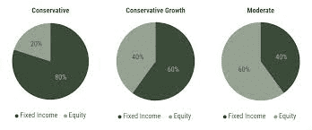
Conventional wisdom has always dictated “not putting all your eggs into one basket.” In more technical terms, this old adage is addressing the benefits of diversification. Markowitz quantified the concept of diversification through the statistical notion of covariance between individual securities, and the overall standard deviation of a portfolio. In essence, the old adage is saying that investing all your money in assets that may all perform poorly at the same time-that is, whose returns are highly correlated-is not a very prudent investment strategy no matter how small the chance that any one asset will perform poorly. This is because if any one single asset performs poorly, it is likely, due to its high correlation with the other assets, that these other assets are also going to perform poorly, leading to the poor performance of the portfolio.

Diversification is related to the Central Limit Theorem, which states that the sum of identical and independent random variables with bounded variance is asymptotically Gaussian. ${ }^2$ In its simplest form, we can formally state this as follows: if $X_1, X_2, \ldots, X_N$ are $N$ independent random variables, each $X_i$ with an arbitrary probability distribution, with finite mean $\mu$ and variance $\sigma^2$, then
$$
\lim {N \rightarrow \infty} P\left(\frac{1}{\sigma \sqrt{N}} \sum{i=1}^N\left(X_i-\mu\right) \leq y\right)=\frac{1}{\sqrt{2 \pi}} \int_{-\infty}^y e^{-\frac{1}{2} s^2} d s
$$
For a portfolio of $N$ identically and independently distributed assets with returns $R_1, R_2, \ldots, R_N$, in each of which we invest an equal amount, the portfolio return
$$
R_p=\frac{1}{N} \sum_{i=1}^N R_i
$$
is a random variable that will be distributed approximately Gaussian when $N$ is sufficiently large. The Central Limit Theorem implies that the variance of this portfolio is
$$
\begin{aligned}
\operatorname{var}\left(R_p\right) &=\frac{1}{N^2} \sum_{i=1}^N \operatorname{var}\left(R_i\right) \
&=\frac{1}{N^2} N \cdot \sigma^2 \
&=\frac{\sigma^2}{N}{\underset{N \rightarrow \infty}{\longrightarrow}}
\end{aligned}
$$

金融代写|投资组合代写Investment Portfolio代考|MEAN-VARIANCE ANALYSIS: OVERVIEW

Markowitz’s starting point is that of a rational investor who, at time $t$, decides what portfolio of investments to hold for a time horizon of $\Delta t$. The investor makes decisions on the gains and losses he will make at time $t+\Delta t$, without considering eventual gains and losses either during or after the period $\Delta$ t. At time $t+\Delta t$, the investor will reconsider the situation and decide anew. This one-period framework is often referred to as myopic (or “short-sighted”) behavior. In general, a myopic investor’s behavior is suboptimal in comparison to an investor who takes a broader approach and makes investment decisions based upon a multiperiod framework. For example, nonmyopic investment strategies are adopted when it is necessary to make trade-offs at future dates between consumption and investment or when significant trading costs related to specific subsets of investments are incurred throughout the holding period.

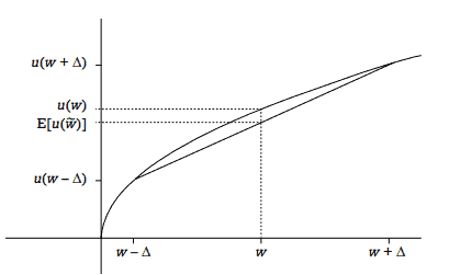
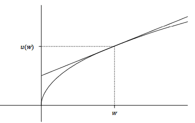
Markowitz reasoned that investors should decide on the basis of a trade-off between risk and expected return. Expected return of a security is defined as the expected price change plus any additional income over the time horizon considered, such as dividend payments, divided by the beginning price of the security. He suggested that risk should be measured by the variance of returns-the average squared deviation around the expected return.

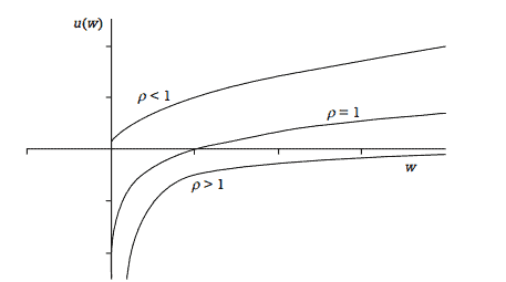
We note that it is a common misunderstanding that Markowitz’s mean-variance framework relies on joint normality of security returns. Markowitz’s mean-variance framework does not assume joint normality of security returns. However, later in this chapter we show that the mean-variance approach is consistent with two different frameworks: (1) expected utility maximization under certain assumptions; or (2) the assumption that security returns are jointly normally distributed.

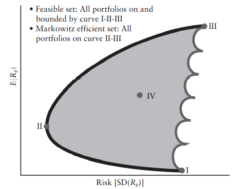
Moreover, Markowitz argued that for any given level of expected return, a rational investor would choose the portfolio with minimum variance from amongst the set of all possible portfolios. The set of all possible portfolios that can be constructed is called the feasible set. Minimum variance portfolios are called mean-variance efficient portfolios. The set of all mean-variance efficient portfolios, for different desired levels of expected return, is called the efficient frontier. Exhibit $2.1$ provides a graphical illustration of the efficient frontier of risky assets. In particular, notice that the feasible set is bounded by the curve I-II-III. All portfolios on the curve II-III are efficient portfolios for different levels of risk. These portfolios offer the lowest level of standard deviation for a given level of expected return. Or equivalently, they constitute the portfolios that maximize expected return for a given level of risk. Therefore, the efficient frontier provides the best possible trade-off between expected return and risk-portfolios below it, such as portfolio IV, are inefficient and portfolios above it are unobtainable.

投资组合代考

金融代写|投资组合代写Investment Portfolio代考|THE BENEFITS OF DIVERSIFICATION

传统智慧总是要求”不要把所有的鸡蛋都放在一个篮子里”。用更专业的术语来说，这句古老的格言是在说明多元 化的好处。马科维茨通过单个证券之间协方差的统计概念和投资组合的整体标准差来量化多元化的概念。从本质 上讲，这句古老的格言是说，将所有资金投资于可能同时表现不佳的资产一一也就是说，其回报高度相关一一并 不是一种非常谨慎的投资策略，无论任何一个人出现这种情况的可能性有多小。资产将表现不佳。这是因为如果 任何一项资产表现不佳，由于其与其他资产的高度相关性，这些其他资产也可能表现不佳，从而导致投资组合表 现不佳。
多样化与中心极限定理有关，该定理指出具有有界方差的相同且独立的随机变量之和呈渐近高斯分布。 ${ }^2$ 以最简 单的形式，我们可以正式地表述如下: 如果 $X_1, X_2, \ldots, X_N$ 是 $N$ 独立随机变量，每个 $X_i$ 具有任意概率分布， 具有有限均值 $\mu$ 和方差 $\sigma^2$ ， 然后
$$
\lim N \rightarrow \infty P\left(\frac{1}{\sigma \sqrt{N}} \sum i=1^N\left(X_i-\mu\right) \leq y\right)=\frac{1}{\sqrt{2 \pi}} \int_{-\infty}^y e^{-\frac{1}{2} s^2} d s
$$
对于一个投资组合 $N$ 具有收益的相同且独立分布的资产 $R_1, R_2, \ldots, R_N$ ，我们在每个投资中投资等量，投资 组合回报
$$
R_p=\frac{1}{N} \sum_{i=1}^N R_i
$$
是一个随机变量，当 $N$ 足够大。中心极限定理意味着这个投资组合的方差是
$$
\operatorname{var}\left(R_p\right)=\frac{1}{N^2} \sum_{i=1}^N \operatorname{var}\left(R_i\right) \quad=\frac{1}{N^2} N \cdot \sigma^2=\frac{\sigma^2}{N} \underset{N \rightarrow \infty}{\longrightarrow}
$$

金融代写|投资组合代写Investment Portfolio代考|MEAN-VARIANCE ANALYSIS: OVERVIEW

马科维茨的出发点是一位理性投资者，他在某个时候吨, 决定在以下时间范围内持有何种投资组合丁吨. 投资者根据他将在某个时间做出的收益和损失做出决定吨+丁吨, 不考虑期中或期后的最终损益丁吨。在时间吨+丁吨, 投资者将重新考虑情况并重新决定。这种一次性框架通常被称为近视（或“短视”）行为。一般来说，与采取更广泛方法并根据多周期框架做出投资决策的投资者相比，短视投资者的行为是次优的。例如，当需要在未来日期在消费和投资之间进行权衡或在整个持有期间产生与特定投资子集相关的重大交易成本时，就会采用非近视投资策略。

马科维茨推断，投资者应该根据风险和预期回报之间的权衡来做出决定。证券的预期回报被定义为预期价格变化加上所考虑时间范围内的任何额外收入，例如股息支付，除以证券的起始价格。他建议风险应该用回报的方差来衡量——即预期回报的平均平方偏差。

我们注意到，马科维茨的均值-方差框架依赖于证券回报的联合正态性，这是一种常见的误解。Markowitz 的均值-方差框架不假设证券收益的联合正态性。然而，在本章后面我们将展示均值-方差方法与两个不同的框架是一致的：（1）某些假设下的预期效用最大化；(2) 证券收益呈联合正态分布的假设。

此外，马科维茨认为，对于任何给定的预期回报水平，理性投资者会从所有可能的投资组合中选择方差最小的投资组合。可以构建的所有可能投资组合的集合称为可行集。最小方差投资组合称为均值-方差有效投资组合。对于不同期望水平的预期回报，所有均值-方差有效投资组合的集合称为有效边界。展示2.1提供了风险资产有效边界的图形说明。特别要注意，可行集以曲线 I-II-III 为界。曲线 II-III 上的所有投资组合都是针对不同风险水平的有效投资组合。这些投资组合为给定的预期回报水平提供最低水平的标准差。或者等价地，它们构成了在给定风险水平下最大化预期回报的投资组合。因此，有效边界在预期收益和低于它的风险投资组合（例如投资组合 IV）之间提供了最好的权衡，它是无效的，高于它的投资组合是无法获得的。

统计代写请认准statistics-lab™. statistics-lab™为您的留学生涯保驾护航。统计代写|python代写代考

随机过程代考

在概率论概念中，随机过程是随机变量的集合。 若一随机系统的样本点是随机函数，则称此函数为样本函数，这一随机系统全部样本函数的集合是一个随机过程。 实际应用中，样本函数的一般定义在时间域或者空间域。 随机过程的实例如股票和汇率的波动、语音信号、视频信号、体温的变化，随机运动如布朗运动、随机徘徊等等。

贝叶斯方法代考

贝叶斯统计概念及数据分析表示使用概率陈述回答有关未知参数的研究问题以及统计范式。后验分布包括关于参数的先验分布，和基于观测数据提供关于参数的信息似然模型。根据选择的先验分布和似然模型，后验分布可以解析或近似，例如，马尔科夫链蒙特卡罗 (MCMC) 方法之一。贝叶斯统计概念及数据分析使用后验分布来形成模型参数的各种摘要，包括点估计，如后验平均值、中位数、百分位数和称为可信区间的区间估计。此外，所有关于模型参数的统计检验都可以表示为基于估计后验分布的概率报表。

广义线性模型代考

广义线性模型（GLM）归属统计学领域，是一种应用灵活的线性回归模型。该模型允许因变量的偏差分布有除了正态分布之外的其它分布。

statistics-lab作为专业的留学生服务机构，多年来已为美国、英国、加拿大、澳洲等留学热门地的学生提供专业的学术服务，包括但不限于Essay代写，Assignment代写，Dissertation代写，Report代写，小组作业代写，Proposal代写，Paper代写，Presentation代写，计算机作业代写，论文修改和润色，网课代做，exam代考等等。写作范围涵盖高中，本科，研究生等海外留学全阶段，辐射金融，经济学，会计学，审计学，管理学等全球99%专业科目。写作团队既有专业英语母语作者，也有海外名校硕博留学生，每位写作老师都拥有过硬的语言能力，专业的学科背景和学术写作经验。我们承诺100%原创，100%专业，100%准时，100%满意。

机器学习代写

随着AI的大潮到来，Machine Learning逐渐成为一个新的学习热点。同时与传统CS相比，Machine Learning在其他领域也有着广泛的应用，因此这门学科成为不仅折磨CS专业同学的“小恶魔”，也是折磨生物、化学、统计等其他学科留学生的“大魔王”。学习Machine learning的一大绊脚石在于使用语言众多，跨学科范围广，所以学习起来尤其困难。但是不管你在学习Machine Learning时遇到任何难题，StudyGate专业导师团队都能为你轻松解决。

多元统计分析代考

基础数据: $N$ 个样本， $P$ 个变量数的单样本，组成的横列的数据表
变量定性: 分类和顺序；变量定量：数值
数学公式的角度分为: 因变量与自变量

时间序列分析代写

随机过程，是依赖于参数的一组随机变量的全体，参数通常是时间。 随机变量是随机现象的数量表现，其时间序列是一组按照时间发生先后顺序进行排列的数据点序列。通常一组时间序列的时间间隔为一恒定值（如1秒，5分钟，12小时，7天，1年），因此时间序列可以作为离散时间数据进行分析处理。研究时间序列数据的意义在于现实中，往往需要研究某个事物其随时间发展变化的规律。这就需要通过研究该事物过去发展的历史记录，以得到其自身发展的规律。

回归分析代写

多元回归分析渐进（Multiple Regression Analysis Asymptotics）属于计量经济学领域，主要是一种数学上的统计分析方法，可以分析复杂情况下各影响因素的数学关系，在自然科学、社会和经济学等多个领域内应用广泛。

MATLAB代写

MATLAB 是一种用于技术计算的高性能语言。它将计算、可视化和编程集成在一个易于使用的环境中，其中问题和解决方案以熟悉的数学符号表示。典型用途包括：数学和计算算法开发建模、仿真和原型制作数据分析、探索和可视化科学和工程图形应用程序开发，包括图形用户界面构建MATLAB 是一个交互式系统，其基本数据元素是一个不需要维度的数组。这使您可以解决许多技术计算问题，尤其是那些具有矩阵和向量公式的问题，而只需用 C 或 Fortran 等标量非交互式语言编写程序所需的时间的一小部分。MATLAB 名称代表矩阵实验室。MATLAB 最初的编写目的是提供对由 LINPACK 和 EISPACK 项目开发的矩阵软件的轻松访问，这两个项目共同代表了矩阵计算软件的最新技术。MATLAB 经过多年的发展，得到了许多用户的投入。在大学环境中，它是数学、工程和科学入门和高级课程的标准教学工具。在工业领域，MATLAB 是高效研究、开发和分析的首选工具。MATLAB 具有一系列称为工具箱的特定于应用程序的解决方案。对于大多数 MATLAB 用户来说非常重要，工具箱允许您学习和应用专业技术。工具箱是 MATLAB 函数（M 文件）的综合集合，可扩展 MATLAB 环境以解决特定类别的问题。可用工具箱的领域包括信号处理、控制系统、神经网络、模糊逻辑、小波、仿真等。

如果你也在 怎样代写投资组合Investment Portfolio这个学科遇到相关的难题，请随时右上角联系我们的24/7代写客服。

投资组合是由投资人或金融机构所持有的股票、债券、金融衍生产品等组成的集合。目的是分散风险。投资组合可以看成几个层面上的组合。

statistics-lab™ 为您的留学生涯保驾护航 在代写投资组合Investment Portfolio方面已经树立了自己的口碑, 保证靠谱, 高质且原创的统计Statistics代写服务。我们的专家在代写投资组合Investment Portfolio方面经验极为丰富，各种代写投资组合Investment Portfolio相关的作业也就用不着说。

我们提供的投资组合Investment Portfolio及其相关学科的代写，服务范围广, 其中包括但不限于:

• Statistical Inference 统计推断
• Statistical Computing 统计计算
• Advanced Probability Theory 高等楖率论
• Advanced Mathematical Statistics 高等数理统计学
• (Generalized) Linear Models 广义线性模型
• Statistical Machine Learning 统计机器学习
• Longitudinal Data Analysis 纵向数据分析
• Foundations of Data Science 数据科学基础

金融代写|投资组合代写Investment Portfolio代考|Computer Technology and the Internet

The appearance of the first personal computers in the late $1970 \mathrm{~s}$ and early 1980 s forever changed the world of computing. It put computational resources within the reach of most people. In a few years every trading desk on Wall Street was equipped with a PC. From that point on, computing costs have declined at the significant pace of about a factor of 2 every year. For example, the cost per gigaflops ${ }^{16}$ is about $\$ 1$ today, to be compared to about $\$ 50,000$ about 10 years ago. ${ }^{17}$ At the same time, computer speed increased in a similar fashion: today’s fastest computers are able to perform an amazing 300 trillion calculations per second. ${ }^{18}$ This remarkable development of computing technology has allowed finance professionals to deploy more sophisticated algorithms used, for instance, for derivative and asset pricing, market forecasting, portfolio allocation, and computerized execution and trading. With state-of-theart optimization software, a portfolio manager is able to calculate the optimal allocation for a portfolio of thousands of assets in no more than a few seconds-on the manager’s desktop computer!
${ }^{15}$ Peter L. Bernstein, Capital Ideas (New York: Free Press, 1993).
${ }^{16}$ Flops is an abbreviation for floating point operations per second and is used as a measure of a computer’s performance. 1 gigaflops $=10^9$ flops.
${ }^{17}$ See Michael S. Warren, John K. Salmon, Donald J. Becker, M. Patrick Goda, Thomas Sterling, and Grégoire S. Winckelmans, “Pentium Pro Inside: I. A Treecode at 430 Gigaflops on ASCI Red. II. Price/Performance of \$50/Mflop on Loki and Hyglac,” Supercomputing ’97, Los Alamitos, 1997, IEEE Computer Society; and Wikipedia contributors, “FLOPS,” Wikipedia, The Free Encyclopedia, http:// en.wikipedia.org/w/index.php?title=FLOPS\&coldid=90585825 (accessed December 1, 2006).
${ }^{18}$ As of November 2006, the IBM BlueGene/L system with 131072 processor units held the so-called Linpack record with a remarkable performance of $280.6$ teraflops (that is, $280.6$ trillions of floating-point operations per second). See TOP500, www.top500.org.

金融代写|投资组合代写Investment Portfolio代考|Capital Markets

The development of the capital markets has of course had a significant impact on quantitative finance and the investment management industry as a whole. Investors today have a vast number of assets available in the capital markets, from more traditional assets such as stocks, bonds, commodities (precious metals, etc.) and real estate to derivative instruments such as options, futures, swaps, credit linked securities, mortgage-backed securities and other structured products, and specialized financial insurance products. These securities and products allow market participants to get exposure to, or to hedge risks-sometimes very specific risks. For example, a corporatè bond portfolio manager may decide to hédgè speecific credit risks in his portfolio using a credit default swap, or a proprietary trader can short equity volatility by selling a volatility swap.

However, the number of assets available alone is not enough to guarantee success, if the assets are only traded infrequently and in small volumes. Successful capital markets have to be liquid, allowing market participants to trade their positions quickly and at low cost. An asset is said to be liquid if it can be converted to cash quickly at a price close to fair market value. The U.S. capital markets are the most liquid in the world with Japan and the United Kingdom following. Cash, being the basic liquid asset, does not fluctuate in value-it itself defines price. All other assets can change in value and have an uncertain future price, making them risky assets. Naturally, informed investors will only hold less liquid and risky assets if they can expect to earn a premium, a risk premium.
With the tremendous increase in the number of assets-and with it, the amount of investment opportunities-it is hard, even for larger investment houses, to track and evaluate the different markets. Quantitative techniques lend themselves for automatic monitoring and analysis of the full multitude of securities. These tools give quantitative analysts, portfolio managers, and other decision makers the opportunity to summarize the vast amount of information available, and to present it in a cohesive manner. Modern financial and the econometric models rely on the access to accurate data, often with as long history as possible. It is typically much easier to obtain clean and trustworthy financial data from mature and liquid markets. In fact, the lack of reliable data is one of the inherent problems in applying sophisticated quantitative models to more illiquid markets. In these cases, practitioners are forced to rely on simulated data, make stronger assumptions in their models, or use less data-intensive models.

投资组合代考

金融代写|投资组合代写Investment Portfolio代考|Computer Technology and the Internet

晚期第一台个人电脑的出现1970 秒20 世纪 80 年代初永远地改变了计算世界。它使大多数人都能获得计算资源。几年后，华尔街的每个交易柜台都配备了个人电脑。从那时起，计算成本每年以大约 2 倍的显着速度下降。例如，每 gigaflops 的成本16是关于$1今天，与大约$50,000大约 10 年前。17与此同时，计算机速度以类似的方式提高：当今最快的计算机每秒能够执行惊人的 300 万亿次计算。18计算技术的这一显着发展使金融专业人士能够部署更复杂的算法，例如用于衍生品和资产定价、市场预测、投资组合分配以及计算机化执行和交易。借助最先进的优化软件，投资组合经理能够在不超过几秒钟的时间内在经理的台式计算机上计算出数千种资产的投资组合的最佳配置！
15Peter L. Bernstein，Capital Ideas（纽约：自由出版社，1993 年）。
16Flops 是每秒浮点运算的缩写，用来衡量计算机的性能。1 千兆浮点数=109拖鞋。
17参见 Michael S. Warren、John K. Salmon、Donald J. Becker、M. Patrick Goda、Thomas Sterling 和 Grégoire S. Winckelmans，“Pentium Pro Inside：I. A Treecode at 430 Gigaflops on ASCI Red。二。Loki 和 Hyglac的价格/性能为 50美元/Mflop，”Supercomputing ’97，Los Alamitos，1997，IEEE 计算机协会；和维基百科贡献者，“FLOPS”，维基百科，免费百科全书，http://en.wikipedia.org/w/index.php?title=FLOPS\&coldid=90585825（2006 年 12 月 1 日访问）。
18截至 2006 年 11 月，拥有 131072 个处理器单元的 IBM BlueGene/L 系统保持着所谓的 Linpack 记录，性能卓越280.6万亿次浮点数（即280.6每秒数万亿次浮点运算）。参见 TOP500，www.top500.org。

金融代写|投资组合代写Investment Portfolio代考|Capital Markets

资本市场的发展当然对量化金融乃至整个投资管理行业产生了重大影响。今天的投资者在资本市场上拥有大量可用资产，从股票、债券、商品（贵金属等）和房地产等更传统的资产到期权、期货、掉期、信用挂钩证券等衍生工具，抵押贷款支持证券和其他结构性产品，以及专门的金融保险产品。这些证券和产品允许市场参与者接触或对冲风险——有时是非常具体的风险。例如，公司债券投资组合经理可能决定使用信用违约互换来对冲其投资组合中的特定信用风险，

然而，如果资产的交易不频繁且交易量很小，仅凭可用资产的数量不足以保证成功。成功的资本市场必须具有流动性，允许市场参与者以低成本快速交易他们的头寸。如果一项资产能够以接近公平市场价值的价格迅速转换为现金，则称该资产具有流动性。美国资本市场是世界上流动性最强的，其次是日本和英国。现金作为基本的流动资产，其价值不会波动——它本身就决定了价格。所有其他资产的价值都可能发生变化，未来价格也不确定，因此成为风险资产。自然地，消息灵通的投资者如果可以预期赚取溢价，即风险溢价，他们只会持有流动性和风险较低的资产。
随着资产数量的急剧增加——随之而来的是投资机会的数量——即使对于较大的投资公司来说，也很难跟踪和评估不同的市场。定量技术有助于自动监控和分析大量证券。这些工具让量化分析师、投资组合经理和其他决策者有机会总结大量可用信息，并以连贯的方式呈现这些信息。现代金融和计量经济学模型依赖于对准确数据的访问，这些数据通常具有尽可能长的历史。从成熟且流动性强的市场获取干净可靠的财务数据通常要容易得多。实际上，缺乏可靠数据是将复杂​​的定量模型应用于流动性较差的市场的固有问题之一。在这些情况下，从业者被迫依赖模拟数据，在他们的模型中做出更强的假设，或者使用较少的数据密集型模型。

统计代写请认准statistics-lab™. statistics-lab™为您的留学生涯保驾护航。统计代写|python代写代考

随机过程代考

在概率论概念中，随机过程是随机变量的集合。 若一随机系统的样本点是随机函数，则称此函数为样本函数，这一随机系统全部样本函数的集合是一个随机过程。 实际应用中，样本函数的一般定义在时间域或者空间域。 随机过程的实例如股票和汇率的波动、语音信号、视频信号、体温的变化，随机运动如布朗运动、随机徘徊等等。

贝叶斯方法代考

贝叶斯统计概念及数据分析表示使用概率陈述回答有关未知参数的研究问题以及统计范式。后验分布包括关于参数的先验分布，和基于观测数据提供关于参数的信息似然模型。根据选择的先验分布和似然模型，后验分布可以解析或近似，例如，马尔科夫链蒙特卡罗 (MCMC) 方法之一。贝叶斯统计概念及数据分析使用后验分布来形成模型参数的各种摘要，包括点估计，如后验平均值、中位数、百分位数和称为可信区间的区间估计。此外，所有关于模型参数的统计检验都可以表示为基于估计后验分布的概率报表。

广义线性模型代考

广义线性模型（GLM）归属统计学领域，是一种应用灵活的线性回归模型。该模型允许因变量的偏差分布有除了正态分布之外的其它分布。

statistics-lab作为专业的留学生服务机构，多年来已为美国、英国、加拿大、澳洲等留学热门地的学生提供专业的学术服务，包括但不限于Essay代写，Assignment代写，Dissertation代写，Report代写，小组作业代写，Proposal代写，Paper代写，Presentation代写，计算机作业代写，论文修改和润色，网课代做，exam代考等等。写作范围涵盖高中，本科，研究生等海外留学全阶段，辐射金融，经济学，会计学，审计学，管理学等全球99%专业科目。写作团队既有专业英语母语作者，也有海外名校硕博留学生，每位写作老师都拥有过硬的语言能力，专业的学科背景和学术写作经验。我们承诺100%原创，100%专业，100%准时，100%满意。

机器学习代写

随着AI的大潮到来，Machine Learning逐渐成为一个新的学习热点。同时与传统CS相比，Machine Learning在其他领域也有着广泛的应用，因此这门学科成为不仅折磨CS专业同学的“小恶魔”，也是折磨生物、化学、统计等其他学科留学生的“大魔王”。学习Machine learning的一大绊脚石在于使用语言众多，跨学科范围广，所以学习起来尤其困难。但是不管你在学习Machine Learning时遇到任何难题，StudyGate专业导师团队都能为你轻松解决。

多元统计分析代考

基础数据: $N$ 个样本， $P$ 个变量数的单样本，组成的横列的数据表
变量定性: 分类和顺序；变量定量：数值
数学公式的角度分为: 因变量与自变量

时间序列分析代写

随机过程，是依赖于参数的一组随机变量的全体，参数通常是时间。 随机变量是随机现象的数量表现，其时间序列是一组按照时间发生先后顺序进行排列的数据点序列。通常一组时间序列的时间间隔为一恒定值（如1秒，5分钟，12小时，7天，1年），因此时间序列可以作为离散时间数据进行分析处理。研究时间序列数据的意义在于现实中，往往需要研究某个事物其随时间发展变化的规律。这就需要通过研究该事物过去发展的历史记录，以得到其自身发展的规律。

回归分析代写

多元回归分析渐进（Multiple Regression Analysis Asymptotics）属于计量经济学领域，主要是一种数学上的统计分析方法，可以分析复杂情况下各影响因素的数学关系，在自然科学、社会和经济学等多个领域内应用广泛。

MATLAB代写

MATLAB 是一种用于技术计算的高性能语言。它将计算、可视化和编程集成在一个易于使用的环境中，其中问题和解决方案以熟悉的数学符号表示。典型用途包括：数学和计算算法开发建模、仿真和原型制作数据分析、探索和可视化科学和工程图形应用程序开发，包括图形用户界面构建MATLAB 是一个交互式系统，其基本数据元素是一个不需要维度的数组。这使您可以解决许多技术计算问题，尤其是那些具有矩阵和向量公式的问题，而只需用 C 或 Fortran 等标量非交互式语言编写程序所需的时间的一小部分。MATLAB 名称代表矩阵实验室。MATLAB 最初的编写目的是提供对由 LINPACK 和 EISPACK 项目开发的矩阵软件的轻松访问，这两个项目共同代表了矩阵计算软件的最新技术。MATLAB 经过多年的发展，得到了许多用户的投入。在大学环境中，它是数学、工程和科学入门和高级课程的标准教学工具。在工业领域，MATLAB 是高效研究、开发和分析的首选工具。MATLAB 具有一系列称为工具箱的特定于应用程序的解决方案。对于大多数 MATLAB 用户来说非常重要，工具箱允许您学习和应用专业技术。工具箱是 MATLAB 函数（M 文件）的综合集合，可扩展 MATLAB 环境以解决特定类别的问题。可用工具箱的领域包括信号处理、控制系统、神经网络、模糊逻辑、小波、仿真等。

如果你也在 怎样代写投资组合Investment Portfolio这个学科遇到相关的难题，请随时右上角联系我们的24/7代写客服。

投资组合是由投资人或金融机构所持有的股票、债券、金融衍生产品等组成的集合。目的是分散风险。投资组合可以看成几个层面上的组合。

statistics-lab™ 为您的留学生涯保驾护航 在代写投资组合Investment Portfolio方面已经树立了自己的口碑, 保证靠谱, 高质且原创的统计Statistics代写服务。我们的专家在代写投资组合Investment Portfolio方面经验极为丰富，各种代写投资组合Investment Portfolio相关的作业也就用不着说。

我们提供的投资组合Investment Portfolio及其相关学科的代写，服务范围广, 其中包括但不限于:

• Statistical Inference 统计推断
• Statistical Computing 统计计算
• Advanced Probability Theory 高等楖率论
• Advanced Mathematical Statistics 高等数理统计学
• (Generalized) Linear Models 广义线性模型
• Statistical Machine Learning 统计机器学习
• Longitudinal Data Analysis 纵向数据分析
• Foundations of Data Science 数据科学基础

金融代写|投资组合代写Investment Portfolio代考|Quadratic Utility

A special case of category (iii) of the shifted power utility function is $\rho=-1$, in which case the utility is
$$
-\frac{1}{2}(w-\zeta)^2=-\frac{1}{2} \zeta^2+\zeta w-\frac{1}{2} w^2 .
$$
This is the case of quadratic utility, which has a special importance in finance theory, because it implies mean-variance preferences. Specifically, the investor’s expected utility is, ignoring the additive constant $-\zeta^2 / 2$,
$$
\zeta \mathrm{E}[\tilde{w}]-\frac{1}{2} \mathrm{E}\left[\tilde{w}^2\right]=\zeta \mathrm{E}[\tilde{w}]-\frac{1}{2} \mathrm{E}[\tilde{w}]^2-\frac{1}{2} \operatorname{var}(\tilde{w}),
$$
where $\operatorname{var}(\tilde{w})$ denotes the variance of $\tilde{w}$. Thus, preferences over gambles depend only on their means and variances when an investor has quadratic utility. Quadratic utility is defined for $w>\zeta$, but it is decreasing in wealth for $w>\zeta$.
If the parameter $\zeta$ is larger than any wealth level the investor could achieve, then it is not a problem that the quadratic utility is decreasing for wealth above $\zeta$. A greater problem with quadratic utility is that it has increasing absolute risk aversion, even for $w<\zeta$. This property of increasing absolute risk aversion (decreasing risk tolerance) is shared by every shifted power utility function with $\rho<0$. As will be seen in Chapter 2 , this implies that risky assets are inferior goods for an investor with quadratic utility: such an investor would invest less in risky assets if her wealth were higher. This is a very unattractive assumption.

金融代写|投资组合代写Investment Portfolio代考|UTILITY AND WEALTH MOMENTS

We can often represent the expected utility of a gamble as an infinite series in the central moments of the gamble’s distribution. Let $w$ denote the mean of a gamble $\tilde{w}$, and suppose the utility function has a convergent Taylor series expansion around $w$. This means that
$u(\tilde{w})=u(w)+u^{\prime}(w)(\tilde{w}-w)+\frac{1}{2} u^{\prime \prime}(w)(\tilde{w}-w)^2+\cdots+\frac{1}{n !} u^{(n)}(w)(\tilde{w}-w)^n+\cdots$
in each state of the world, where $u^{(n)}$ denotes the $n$th derivative of the utility function (for convenience, we are using both this notation and primes to denote derivatives here). Assuming we can interchange expectation with the limit in the infinite series, we obtain
$$
\mathrm{E}[u(\tilde{w})]=u(w)+\frac{1}{2} u^{\prime \prime}(w) \mathrm{E}\left[(\tilde{w}-w)^2\right]+\sum_{n=3}^{\infty} \frac{1}{n !} u^{(n)}(w) \mathrm{E}\left[(\tilde{w}-w)^n\right] .
$$
Risk aversion implies that $u^{\prime \prime}(w)<0$, so, in view of the formula (1.16), it is reasonable to say that a risk-averse investor dislikes variance. As mentioned in Section 1.1, the third derivative of a DAR A utility function is positive. Therefore, the coefficient on the third central moment $\mathrm{E}\left[(\tilde{w}-w)^3\right]$ is positive in (1.16). The third central moment divided by the standard deviation cubed is called skewness. Therefore, it is reasonable to say that an investor with DARA utility prefers positive skewness to negative skewness. As mentioned in Section 1.1, the combination of DARA utility and decreasing absolute prudence implies that the fourth derivative of the utility function is negative. The fourth central moment divided by the variance squared is called kurtosis (sometimes 3 is subtracted, in which case normal distributions have zero kurtosis). So, it is reasonable to say that decreasing absolute prudence implies a dislike of kurtosis.

It is tempting to truncate the infinite sum in (1.16) and to argue that we can approximate expected utility by a function of a finite number of central moments. However, this is dangerous to do. For most utility functions, and absent any restrictions on the distributions of gambles being considered, any function of a finite number (say $n$ ) of central moments will fail to represent preferences, in the sense that there exist two gambles with all of the first $n$ moments indicating one preference, whereas the actual expected utilities imply the opposite preference. See Section $1.6$ and Exercise $1.4$ for further information on this point. Of course, expected quadratic utility depends only on the first two central moments, as discussed in the previous section, and, if only normal distributions are being considered, then expected utility again depends on only the first two central moments (see the end-of-chapter notes for further discussion of this point).

投资组合代考

金融代写|投资组合代写Investment Portfolio代考|Quadratic Utility

移位功率效用函数的类别 (iii) 的一个特例是 $\rho=-1$ ，在这种情况下，效用是
$$
-\frac{1}{2}(w-\zeta)^2=-\frac{1}{2} \zeta^2+\zeta w-\frac{1}{2} w^2 .
$$
这就是二次效用的情况，它在金融理论中具有特殊的重要性，因为它暗示了均值方差偏好。具体来说，投资者的 预期效用是，忽略加性常数 $-\zeta^2 / 2$ ，
$$
\zeta \mathrm{E}[\tilde{w}]-\frac{1}{2} \mathrm{E}\left[\tilde{w}^2\right]=\zeta \mathrm{E}[\tilde{w}]-\frac{1}{2} \mathrm{E}[\tilde{w}]^2-\frac{1}{2} \operatorname{var}(\tilde{w}),
$$
在哪里 $\operatorname{var}(\tilde{w})$ 表示方差 $\tilde{w}$. 因此，当投资者具有二次效用时，对赌博的偏好仅取决于它们的均值和方差。二次效 用定义为 $w>\zeta$ ，但它的财富正在减少 $w>\zeta$.
如果参数 $\zeta$ 大于投资者所能达到的任何财富水平，那么当财富高于 $\zeta$. 二次效用的一个更大的问题是它具有增加的 绝对风险厌恶程度，即使对于 $w<\zeta$. 这种增加绝对风险厌恶（降低风险承受能力）的特性由每个转移的募效用 函数共享 $\rho<0$. 正如将在第 2 章中看到的那样，这意味着对于具有二次效用的投资者而言，风险资产是劣质商 品: 如果她的财富较高，这样的投资者将较少投资于风险资产。这是一个非常没有吸引力的假设。

金融代写|投资组合代写Investment Portfolio代考|UTILITY AND WEALTH MOMENTS

我们通常可以将赌博的预期效用表示为赌博分布中心时刻的无限级数。让 $w$ 表示赌博的平均值 $\tilde{w}1$ ，并假设效用函 数有一个收敛的泰勒级数展开 $w$. 这意味着 $u(\tilde{w})=u(w)+u^{\prime}(w)(\tilde{w}-w)+\frac{1}{2} u^{\prime \prime}(w)(\tilde{w}-w)^2+\cdots+\frac{1}{n !} u^{(n)}(w)(\tilde{w}-w)^n+\cdots$ 在世界的每个州，其中 $u^{(n)}$ 表示 $n$ 效用函数的 th 导数（为方便起见，我们在这里使用这个符号和素数来表示导 数）。假设我们可以将期望与无限级数中的极限互换，我们得到 $$ \mathrm{E}[u(\tilde{w})]=u(w)+\frac{1}{2} u^{\prime \prime}(w) \mathrm{E}\left[(\tilde{w}-w)^2\right]+\sum{n=3}^{\infty} \frac{1}{n !} u^{(n)}(w) \mathrm{E}\left[(\tilde{w}-w)^n\right] .
$$
风险厈恶意味着 $u^{\prime \prime}(w)<0$ ，因此，鉴于公式 (1.16)，可以合理地说厌恶风险的投资者不喜欢方差。如 $1.1$ 节所述，DAR A 效用函数的三阶导数为正。因此，第三个中心矩上的系数 $\mathrm{E}\left[(\tilde{w}-w)^3\right]$ 在 (1.16) 中为正。第 三个中心矩除以标准差的立方称为偏度。因此，可以合理地说，拥有 DARA 效用的投资者更喜欢正偏度而不是 负偏度。如第 $1.1$ 节所述，DARA 效用和递减绝对谨慎性的组合意味着效用函数的四阶导数为负。除以方差平方 的第四个中心矩称为峰态 (有时减去 3，在这种情况下，正态分布的峰态为零)。因此，可以合理地说，减少绝 对谨慎意味着不喜欢峰态。
截断 (1.16) 中的无限和并认为我们可以通过有限数量的中心矩的函数来近似预期效用是很诱人的。但是，这样 做很危险。对于大多数效用函数，并且对所考虑的赌博分布没有任何限制，任何有限数的函数 (例如 $n$ ) 的中心 时刻将无法代表偏好，因为存在两个赌博，所有第一个 $n$ 时刻表示一种偏好，而实际预期效用则暗示相反的偏 好。见部分 $1.6$ 和锻炼 $1.4$ 有关这一点的更多信息。当然，预期二次效用仅取决于前两个中心矩，如上一节所 述，如果只考虑正态分布，那么预期效用再次仅取决于前两个中心矩（见- 章节注释以进一步讨论这一点）。

统计代写请认准statistics-lab™. statistics-lab™为您的留学生涯保驾护航。统计代写|python代写代考

随机过程代考

在概率论概念中，随机过程是随机变量的集合。 若一随机系统的样本点是随机函数，则称此函数为样本函数，这一随机系统全部样本函数的集合是一个随机过程。 实际应用中，样本函数的一般定义在时间域或者空间域。 随机过程的实例如股票和汇率的波动、语音信号、视频信号、体温的变化，随机运动如布朗运动、随机徘徊等等。

贝叶斯方法代考

贝叶斯统计概念及数据分析表示使用概率陈述回答有关未知参数的研究问题以及统计范式。后验分布包括关于参数的先验分布，和基于观测数据提供关于参数的信息似然模型。根据选择的先验分布和似然模型，后验分布可以解析或近似，例如，马尔科夫链蒙特卡罗 (MCMC) 方法之一。贝叶斯统计概念及数据分析使用后验分布来形成模型参数的各种摘要，包括点估计，如后验平均值、中位数、百分位数和称为可信区间的区间估计。此外，所有关于模型参数的统计检验都可以表示为基于估计后验分布的概率报表。

广义线性模型代考

广义线性模型（GLM）归属统计学领域，是一种应用灵活的线性回归模型。该模型允许因变量的偏差分布有除了正态分布之外的其它分布。

statistics-lab作为专业的留学生服务机构，多年来已为美国、英国、加拿大、澳洲等留学热门地的学生提供专业的学术服务，包括但不限于Essay代写，Assignment代写，Dissertation代写，Report代写，小组作业代写，Proposal代写，Paper代写，Presentation代写，计算机作业代写，论文修改和润色，网课代做，exam代考等等。写作范围涵盖高中，本科，研究生等海外留学全阶段，辐射金融，经济学，会计学，审计学，管理学等全球99%专业科目。写作团队既有专业英语母语作者，也有海外名校硕博留学生，每位写作老师都拥有过硬的语言能力，专业的学科背景和学术写作经验。我们承诺100%原创，100%专业，100%准时，100%满意。

机器学习代写

随着AI的大潮到来，Machine Learning逐渐成为一个新的学习热点。同时与传统CS相比，Machine Learning在其他领域也有着广泛的应用，因此这门学科成为不仅折磨CS专业同学的“小恶魔”，也是折磨生物、化学、统计等其他学科留学生的“大魔王”。学习Machine learning的一大绊脚石在于使用语言众多，跨学科范围广，所以学习起来尤其困难。但是不管你在学习Machine Learning时遇到任何难题，StudyGate专业导师团队都能为你轻松解决。

多元统计分析代考

基础数据: $N$ 个样本， $P$ 个变量数的单样本，组成的横列的数据表
变量定性: 分类和顺序；变量定量：数值
数学公式的角度分为: 因变量与自变量

时间序列分析代写

随机过程，是依赖于参数的一组随机变量的全体，参数通常是时间。 随机变量是随机现象的数量表现，其时间序列是一组按照时间发生先后顺序进行排列的数据点序列。通常一组时间序列的时间间隔为一恒定值（如1秒，5分钟，12小时，7天，1年），因此时间序列可以作为离散时间数据进行分析处理。研究时间序列数据的意义在于现实中，往往需要研究某个事物其随时间发展变化的规律。这就需要通过研究该事物过去发展的历史记录，以得到其自身发展的规律。

回归分析代写

多元回归分析渐进（Multiple Regression Analysis Asymptotics）属于计量经济学领域，主要是一种数学上的统计分析方法，可以分析复杂情况下各影响因素的数学关系，在自然科学、社会和经济学等多个领域内应用广泛。

MATLAB代写

MATLAB 是一种用于技术计算的高性能语言。它将计算、可视化和编程集成在一个易于使用的环境中，其中问题和解决方案以熟悉的数学符号表示。典型用途包括：数学和计算算法开发建模、仿真和原型制作数据分析、探索和可视化科学和工程图形应用程序开发，包括图形用户界面构建MATLAB 是一个交互式系统，其基本数据元素是一个不需要维度的数组。这使您可以解决许多技术计算问题，尤其是那些具有矩阵和向量公式的问题，而只需用 C 或 Fortran 等标量非交互式语言编写程序所需的时间的一小部分。MATLAB 名称代表矩阵实验室。MATLAB 最初的编写目的是提供对由 LINPACK 和 EISPACK 项目开发的矩阵软件的轻松访问，这两个项目共同代表了矩阵计算软件的最新技术。MATLAB 经过多年的发展，得到了许多用户的投入。在大学环境中，它是数学、工程和科学入门和高级课程的标准教学工具。在工业领域，MATLAB 是高效研究、开发和分析的首选工具。MATLAB 具有一系列称为工具箱的特定于应用程序的解决方案。对于大多数 MATLAB 用户来说非常重要，工具箱允许您学习和应用专业技术。工具箱是 MATLAB 函数（M 文件）的综合集合，可扩展 MATLAB 环境以解决特定类别的问题。可用工具箱的领域包括信号处理、控制系统、神经网络、模糊逻辑、小波、仿真等。

如果你也在 怎样代写投资组合Investment Portfolio这个学科遇到相关的难题，请随时右上角联系我们的24/7代写客服。

投资组合是由投资人或金融机构所持有的股票、债券、金融衍生产品等组成的集合。目的是分散风险。投资组合可以看成几个层面上的组合。

statistics-lab™ 为您的留学生涯保驾护航 在代写投资组合Investment Portfolio方面已经树立了自己的口碑, 保证靠谱, 高质且原创的统计Statistics代写服务。我们的专家在代写投资组合Investment Portfolio方面经验极为丰富，各种代写投资组合Investment Portfolio相关的作业也就用不着说。

我们提供的投资组合Investment Portfolio及其相关学科的代写，服务范围广, 其中包括但不限于:

• Statistical Inference 统计推断
• Statistical Computing 统计计算
• Advanced Probability Theory 高等楖率论
• Advanced Mathematical Statistics 高等数理统计学
• (Generalized) Linear Models 广义线性模型
• Statistical Machine Learning 统计机器学习
• Longitudinal Data Analysis 纵向数据分析
• Foundations of Data Science 数据科学基础

金融代写|投资组合代写Investment Portfolio代考|LINEAR RISK TOLERANCE

A large amount of financial research is based on a special class of utility functions. This is the class of utility functions having linear risk tolerance (LRT), meaning that the risk tolerance at wealth $w$ is
$$
\tau(w)=A+B w
$$
for some constants $A$ and $B .^6$ The parameter $B$ is called the cautiousness parameter. We also say that these utility functions have hyperbolic absolute risk aversion (HARA), due to the fact that the graph of the function
$$
\alpha(w)=\frac{1}{A+B w} .
$$
is a hyperbola. Note that any LRT utility function with a positive cautiousness parameter has increasing risk tolerance and therefore decreasing absolute risk aversion.

This class of functions contains two important subclasses: the class of utility functions having constant absolute risk aversion (CARA) and the class of utility functions having constant relative risk aversion (CRRA)
Constant Absolute Risk Aversion
Constant absolute risk aversion means that absolute risk aversion is the same at every wealth level. Thus, risk tolerance is $\tau(w)=A=1 / \alpha$, where $\alpha$ is absolute risk aversion. It is left as an exercise (Exercise 1.12) to demonstrate that every CARA utility function is a monotone affine transform of the utility function
$$
u(w)=-\mathrm{e}^{-\alpha w},
$$
where $\alpha$ is a constant and equal to the absolute risk aversion. This is called negative exponential utility.

金融代写|投资组合代写Investment Portfolio代考|Constant Relative Risk Aversion

Constant relative aversion means that relative risk aversion is the same at all wealth levels. Let $\rho$ denote the relative risk aversion. Then, absolute risk aversion is $\rho / w$, so risk tolerance is $\tau(w)=B w=w / \rho$. Note that any CRRA utility function (with positive risk aversion) is a DARA utility function.

Any monotone CRRA utility function is a monotone affine transform of one of the following functions (Exercise 1.12): (i) $u(w)=\log w$, where $\log$ is the natural logarithm, (ii) $u(w)$ equals a positive power, less than one, of $w$, or (iii) $u(w)$ equals minus a negative power of $w$. The last two cases (power utility) can be consolidated by writing
$$
u(w)=\frac{1}{\gamma} w^\gamma
$$
where $\gamma<1$ and $\gamma \neq 0$. A slightly more convenient formulation, which we will adopt, is to write $$ u(w)=\frac{1}{1-\rho} w^{1-\rho} $$ where $\rho=1-\gamma$ is a positive constant different from 1 . We can easily check that $\rho$ is the coefficient of relative risk aversion of the utility function (1.14). Logarithmic utility has constant relative risk aversion equal to 1 , and an investor with power utility (1.14) is said to be more risk averse than a log-utility investor if $\rho>1$ and to be less risk averse than a log-utility investor if $\rho<1$. The three cases $\rho>1, \rho-1$, and $\rho<1$ are illustrated in Figure 1.4.

The fraction of wealth an individual with CRRA utility would pay to avoid a gamble that is proportional to initial wealth is independent of the individual’s wealth. To see this, let $\tilde{\varepsilon}$ be a zero-mean gamble. An individual will pay $\pi w$ to avoid the gamble $\tilde{\varepsilon} w$ if
$$
u((1-\pi) w)=\mathrm{E}[u((1+\tilde{\varepsilon}) w)] .
$$

投资组合代考

金融代写|投资组合代写Investment Portfolio代考|LINEAR RISK TOLERANCE

大量的金融研究是基于一类特殊的效用函数。这是一类具有线性风险承受能力 (LRT) 的效用函数，这意味着财富 的风险承受能力 $w$ 是
$$
\tau(w)=A+B w
$$
对于一些常数 $A$ 和 $B .^6{ }^6$ 参数 $B$ 称为谨慎参数。我们还说这些效用函数具有双曲线绝对风险厌恶 (HARA)，因为 函数的图形
$$
\alpha(w)=\frac{1}{A+B w} .
$$
是双曲线。请注意，任何具有正谨慎参数的 LRT 效用函数都会增加风险承受能力，因此会降低绝对风险厌恶程 度。
此类函数包含两个重要的子类: 具有恒定绝对风险厌恶 (CARA) 的效用函数类和具有恒定相对风险厌恶 (CRRA) 的实用函数类
恒定绝对风险厌恶
恒定绝对风险厌恶意味着绝对风险厌恶是每个财富水平都一样。因此，风险承受能力是 $\tau(w)=A=1 / \alpha$ ，在 哪里 $\alpha$ 是绝对的风险厌恶。它作为一个练习 (练习 1.12) 来证明每个 CARA 效用函数都是效用函数的单调仿射 变换
$$
u(w)=-\mathrm{e}^{-\alpha w},
$$
在哪里 $\alpha$ 是一个常数，等于绝对风险厌恶。这称为负指数效用。

金融代写|投资组合代写Investment Portfolio代考|Constant Relative Risk Aversion

恒定的相对厌恶意味着相对风险厌恶在所有财富水平上都是相同的。让 $\rho$ 表示相对风险厌恶。那么，绝对风险厌 恶是 $\rho / w$ ，所以风险承受能力是 $\tau(w)=B w=w / \rho$. 请注意，任何 CRRA 效用函数 (具有正风险厌恶) 都是 DARA 效用函数。
任何单调 CRRA 效用函数都是以下函数之一的单调仿射变换（练习 1.12）： (i) $u(w)=\log w$ ，在哪里 $\log$ 是 自然对数， (ii) $u(w)$ 等于小于一的正幂 $w$ ，或 (iii) $u(w)$ 等于减去负幂 $w$. 最后两种情况 (电力公用事业) 可以通过 编写合并
$$
u(w)=\frac{1}{\gamma} w^\gamma
$$
在哪里 $\gamma<1$ 和 $\gamma \neq 0$. 我们将采用的一个稍微方便一点的表述是: $$ u(w)=\frac{1}{1-\rho} w^{1-\rho} $$ 在哪里 $\rho=1-\gamma$ 是一个不同于 1 的正常数。我们可以很容易地检查 $\rho$ 是效用函数 (1.14) 的相对风险庆恶系数。 对数效用具有等于 1 的恒定相对风险厌恶，如果满足以下条件，则具有电力效用 (1.14) 的投资者比对数效用投 资者更厌恶风险 $\rho>1$ 并且比对数效用投资者的风险厌恶程度更低，如果 $\rho<1$. 三种情况 $\rho>1, \rho-1$ ，和 $\rho<1$ 如图 $1.4$ 所示。
拥有 CRRA 效用的个人为避免与初始财富成比例的赌博而支付的财富比例与个人的财富无关。要看到这一点，让 $\tilde{\varepsilon}$ 是一个零均值赌博。个人将支付 $\pi w$ 避免赌博 $\tilde{\varepsilon} w$ 如果
$$
u((1-\pi) w)=\mathrm{E}[u((1+\tilde{\varepsilon}) w)]
$$

统计代写请认准statistics-lab™. statistics-lab™为您的留学生涯保驾护航。统计代写|python代写代考

随机过程代考

在概率论概念中，随机过程是随机变量的集合。 若一随机系统的样本点是随机函数，则称此函数为样本函数，这一随机系统全部样本函数的集合是一个随机过程。 实际应用中，样本函数的一般定义在时间域或者空间域。 随机过程的实例如股票和汇率的波动、语音信号、视频信号、体温的变化，随机运动如布朗运动、随机徘徊等等。

贝叶斯方法代考

贝叶斯统计概念及数据分析表示使用概率陈述回答有关未知参数的研究问题以及统计范式。后验分布包括关于参数的先验分布，和基于观测数据提供关于参数的信息似然模型。根据选择的先验分布和似然模型，后验分布可以解析或近似，例如，马尔科夫链蒙特卡罗 (MCMC) 方法之一。贝叶斯统计概念及数据分析使用后验分布来形成模型参数的各种摘要，包括点估计，如后验平均值、中位数、百分位数和称为可信区间的区间估计。此外，所有关于模型参数的统计检验都可以表示为基于估计后验分布的概率报表。

广义线性模型代考

广义线性模型（GLM）归属统计学领域，是一种应用灵活的线性回归模型。该模型允许因变量的偏差分布有除了正态分布之外的其它分布。

statistics-lab作为专业的留学生服务机构，多年来已为美国、英国、加拿大、澳洲等留学热门地的学生提供专业的学术服务，包括但不限于Essay代写，Assignment代写，Dissertation代写，Report代写，小组作业代写，Proposal代写，Paper代写，Presentation代写，计算机作业代写，论文修改和润色，网课代做，exam代考等等。写作范围涵盖高中，本科，研究生等海外留学全阶段，辐射金融，经济学，会计学，审计学，管理学等全球99%专业科目。写作团队既有专业英语母语作者，也有海外名校硕博留学生，每位写作老师都拥有过硬的语言能力，专业的学科背景和学术写作经验。我们承诺100%原创，100%专业，100%准时，100%满意。

机器学习代写

随着AI的大潮到来，Machine Learning逐渐成为一个新的学习热点。同时与传统CS相比，Machine Learning在其他领域也有着广泛的应用，因此这门学科成为不仅折磨CS专业同学的“小恶魔”，也是折磨生物、化学、统计等其他学科留学生的“大魔王”。学习Machine learning的一大绊脚石在于使用语言众多，跨学科范围广，所以学习起来尤其困难。但是不管你在学习Machine Learning时遇到任何难题，StudyGate专业导师团队都能为你轻松解决。

多元统计分析代考

基础数据: $N$ 个样本， $P$ 个变量数的单样本，组成的横列的数据表
变量定性: 分类和顺序；变量定量：数值
数学公式的角度分为: 因变量与自变量

时间序列分析代写

随机过程，是依赖于参数的一组随机变量的全体，参数通常是时间。 随机变量是随机现象的数量表现，其时间序列是一组按照时间发生先后顺序进行排列的数据点序列。通常一组时间序列的时间间隔为一恒定值（如1秒，5分钟，12小时，7天，1年），因此时间序列可以作为离散时间数据进行分析处理。研究时间序列数据的意义在于现实中，往往需要研究某个事物其随时间发展变化的规律。这就需要通过研究该事物过去发展的历史记录，以得到其自身发展的规律。

回归分析代写

多元回归分析渐进（Multiple Regression Analysis Asymptotics）属于计量经济学领域，主要是一种数学上的统计分析方法，可以分析复杂情况下各影响因素的数学关系，在自然科学、社会和经济学等多个领域内应用广泛。

MATLAB代写

MATLAB 是一种用于技术计算的高性能语言。它将计算、可视化和编程集成在一个易于使用的环境中，其中问题和解决方案以熟悉的数学符号表示。典型用途包括：数学和计算算法开发建模、仿真和原型制作数据分析、探索和可视化科学和工程图形应用程序开发，包括图形用户界面构建MATLAB 是一个交互式系统，其基本数据元素是一个不需要维度的数组。这使您可以解决许多技术计算问题，尤其是那些具有矩阵和向量公式的问题，而只需用 C 或 Fortran 等标量非交互式语言编写程序所需的时间的一小部分。MATLAB 名称代表矩阵实验室。MATLAB 最初的编写目的是提供对由 LINPACK 和 EISPACK 项目开发的矩阵软件的轻松访问，这两个项目共同代表了矩阵计算软件的最新技术。MATLAB 经过多年的发展，得到了许多用户的投入。在大学环境中，它是数学、工程和科学入门和高级课程的标准教学工具。在工业领域，MATLAB 是高效研究、开发和分析的首选工具。MATLAB 具有一系列称为工具箱的特定于应用程序的解决方案。对于大多数 MATLAB 用户来说非常重要，工具箱允许您学习和应用专业技术。工具箱是 MATLAB 函数（M 文件）的综合集合，可扩展 MATLAB 环境以解决特定类别的问题。可用工具箱的领域包括信号处理、控制系统、神经网络、模糊逻辑、小波、仿真等。

如果你也在 怎样代写投资组合Investment Portfolio这个学科遇到相关的难题，请随时右上角联系我们的24/7代写客服。

投资组合是由投资人或金融机构所持有的股票、债券、金融衍生产品等组成的集合。目的是分散风险。投资组合可以看成几个层面上的组合。

statistics-lab™ 为您的留学生涯保驾护航 在代写投资组合Investment Portfolio方面已经树立了自己的口碑, 保证靠谱, 高质且原创的统计Statistics代写服务。我们的专家在代写投资组合Investment Portfolio方面经验极为丰富，各种代写投资组合Investment Portfolio相关的作业也就用不着说。

我们提供的投资组合Investment Portfolio及其相关学科的代写，服务范围广, 其中包括但不限于:

• Statistical Inference 统计推断
• Statistical Computing 统计计算
• Advanced Probability Theory 高等楖率论
• Advanced Mathematical Statistics 高等数理统计学
• (Generalized) Linear Models 广义线性模型
• Statistical Machine Learning 统计机器学习
• Longitudinal Data Analysis 纵向数据分析
• Foundations of Data Science 数据科学基础

金融代写|投资组合代写Investment Portfolio代考|UTILITY FUNCTIONS AND RISK AVERSION

A utility function $u$ is said to represent preferences over wealth gambles if $\mathrm{E}\left[u\left(\tilde{w}_1\right)\right] \geq \mathrm{E}\left[u\left(\tilde{w}_2\right)\right]$ for any random $\tilde{w}_1$ and $\tilde{w}_2$ such that $\tilde{w}_1$ is at least as preferred as $\tilde{w}_2$. When making decisions under certainty, the utility function representing preferences is unique only up to monotone transforms. However, for decisions under uncertainty, utility functions are unique up to monotone affine transforms: If two utility functions $u$ and $f$ represent the same preferences over all wealth gambles, then $u$ must be a monotone affine transform of $f$; that is, there exist a constant $a$ and a constant $b>0$ such that $u(w)=a+b f(w)$ for every $w$.

An investor is said to be (weakly) risk averse if
$$
u(w) \geq \mathrm{E}[u(\tilde{w})]
$$
for any random $\tilde{w}$ with mean $w$. An equivalent definition is that a risk-averse investor would prefer to avoid a fair bet, meaning that if $\tilde{\varepsilon}$ is a zero-mean random variable and $w$ is a constant, then
$$
u(w) \geq \mathrm{E}[u(w+\tilde{\varepsilon})] .
$$
These inequalities are known as Jensen’s inequality. They are equivalent to concavity of the utility function. ${ }^2$ Concavity is preserved by monotone affine transforms (though not by general monotone transforms), so, for given preferences, either all utility functions representing the preferences are concave or none are,

Strict concavity is equivalent to strict risk aversion, meaning strict preference for a sure thing over a gamble with the same mean (strict inequality in (1.1) and (1.2), unless $\tilde{w}=w$ or $\tilde{\varepsilon}=0$ with probability 1). For a differentiable function $u$, concavity is equivalent to nonincreasing marginal utility $\left(u^{\prime}\left(w_1\right) \leq u^{\prime}\left(w_0\right)\right.$ if $\left.w_1>w_0\right)$, and strict concavity is equivalent to decreasing marginal utility $\left(u^{\prime}\left(w_1\right)w_0$ ). For a twice differentiable function $u$, concavity is equivalent to $u^{\prime \prime}(w) \leq 0$ for all $w$, and strict concavity is implied by $u^{\prime \prime}(w)<0$ for all $w$.

Figures $1.1$ and $1.2$ illustrate the relationship between concavity and risk aversion. Figure $1.1$ considers a simple two-outcome gamble and uses the definition of concavity to deduce that an investor with concave utility would prefer the mean of the gamble. Figure $1.2$ sketches the proof of Jensen’s inequality, using the fact that a tangent line to the graph of a concave function lies above the graph of the function.

金融代写|投资组合代写Investment Portfolio代考|CERTAINTY EQUIVALENTS AND SECOND-ORDER RISK AVERSION

Let $w$ be the mean of a random $\tilde{w}$, so $\tilde{w}=w+\tilde{\varepsilon}$, where $\mathrm{E}[\tilde{\varepsilon}]=0$. A constant $x$ is said to be the certainty equivalent of $\tilde{w}$ for an individual with utility function $u$ if
$$
u(x)=\mathrm{E}[u(w+\tilde{\varepsilon})]
$$
A constant $\pi$ is said to be the risk premium of $\tilde{w}$ if $w-\pi$ is the certainty equivalent, that is,
$$
(w-\pi)=\mathrm{E}[u(w+\tilde{\varepsilon})] .
$$
In other words, starting at wealth $w, \pi$ is the largest amount the individual would pay to avoid the gamble $\tilde{\varepsilon}_{.}^4$ This concept is illustrated in Figure $1.3$.

We will show that at the end of the section that, for small gambles,
$$
\pi \approx \frac{1}{2} \sigma^2 \alpha(w),
$$
where $\sigma^2$ is the variance of $\tilde{\varepsilon}$. Thus, the amount an investor would pay to avoid the gamble is approximately proportional to her coefficient of absolute risk aversion. The meaning of the approximation is that $\pi / \sigma^2 \rightarrow \alpha(w) / 2$ if we consider a sequence of gambles with variances $\sigma^2 \rightarrow 0$. The approximation is derived at the end of this section.

The distinction between absolute and relative risk aversion can be seen by contrasting (1.4) with the following: Let $\pi=v w$ be the risk premium of $w+w \tilde{\varepsilon}$, where $w$ is a constant and $\tilde{\varepsilon}$ is a zero-mean random variable with variance $\sigma^2$. Then,
$$
v \approx \frac{1}{2} \sigma^2 \rho(w) .
$$
Thus, the proportion $v$ of initial wealth $w$ that an investor would pay to avoid a gamble equal to the proportion $\tilde{\varepsilon}$ of initial wealth depends on her relative risk aversion and the variance of $\tilde{\varepsilon}$. The result (1.5) follows immediately from (1.4): Let $w \tilde{\varepsilon}$ be the gamble we considered when discussing absolute risk aversion; then, the variance of the gamble is $w^2 \sigma^2$; thus,
$$
\pi \approx \frac{1}{2} w^2 \sigma^2 \alpha(w) \quad \Leftrightarrow \quad v \approx \frac{1}{2} w \sigma^2 \alpha(w)=\frac{1}{2} \sigma^2 \rho(w) .
$$

投资组合代考

金融代写|投资组合代写Investment Portfolio代考|UTILITY FUNCTIONS AND RISK AVERSION

效用函数 $u$ 据说代表对财富赌博的偏好，如果 $\mathrm{E}\left[u\left(\tilde{w}_1\right)\right] \geq \mathrm{E}\left[u\left(\tilde{w}_2\right)\right]$ 对于任何随机 $\tilde{w}_1$ 和 $\tilde{w}_2$ 这样 $\tilde{w}_1$ 至少与 $\tilde{w}_2$. 在确定性下做出决策时，表示偏好的效用函数仅在单调变换中是唯一的。然而，对于不确定条件下的决策， 效用函数对于单调仿射变换是唯一的: 如果两个效用函数 $u$ 和 $f$ 代表对所有财富赌博的相同偏好，则 $u$ 必须是单 调仿射变换 $f$; 也就是说，存在一个常数 $a$ 和一个常数 $b>0$ 这样 $u(w)=a+b f(w)$ 对于每个 $w$.
如果满足以下条件，则称投资者 (弱) 风险厌恶
$$
u(w) \geq \mathrm{E}[u(\tilde{w})]
$$
对于任何随机 $\tilde{w}$ 平均 $w$. 一个等效的定义是规避风险的投资者更愿意避免公平的赌注，这意味着如果 $\tilde{\varepsilon}$ 是一个零均 值随机变量，并且 $w$ 是一个常数，那么
$$
u(w) \geq \mathbf{E}[u(w+\tilde{\varepsilon})] .
$$
这些不等式被称为 Jensen 不等式。它们等价于效用函数的凹度。 ${ }^2$ 凹度由单调仿射变换保留（尽管不是通过一 般单调变换)，因此，对于给定的偏好，表示偏好的所有效用函数都是凹的，或者没有，
严格的凹度等同于严格的风险规避，意味着严格偏好确定的事物而不是具有相同均值的赌博（(1.1) 和（1.2) 中的严格不等式，除非 $\tilde{w}=w$ 或者 $\tilde{\varepsilon}=0$ 概率为 1)。对于可微函数 $u$ ，凹度等价于边际效用不增加 $\left(u^{\prime}\left(w_1\right) \leq u^{\prime}\left(w_0\right)\right.$ 如果 $\left.w_1>w_0\right)$ ，严格的凹度等价于边际效用递减 Veft(u^{lprime}Neft(W_1 right)W_0 ) 。对 于二次可微函数 $u$ ，凹度等价于 $u^{\prime \prime}(w) \leq 0$ 对所有人 $w$ ，并且严格的凹度由下式隐含 $u^{\prime \prime}(w)<0$ 对所有人 $w$.
数字 $1.1$ 和 $1.2$ 说明凹度和风险规避之间的关系。数字 $1.1$ 考虑一个简单的两个结果博変，并使用凹度的定义来推 断具有凹效用的投资者更喜欢博亦的均值。数字 $1.2$ 使用凹函数图形的切线位于函数图形上方这一事实，勾勒出 Jensen 不等式的证明。

金融代写|投资组合代写Investment Portfolio代考|CERTAINTY EQUIVALENTS AND SECOND-ORDER RISK AVERSION

让 $w$ 是随机的平均值 $\tilde{w}$ ，所以 $\tilde{w}=w+\tilde{\varepsilon}$ ，在哪里 $\mathrm{E}[\tilde{\varepsilon}]=0$. 一个常数 $x$ 据说是确定性等价于 $\tilde{w}$ 对于具有效用 函数的个人 $u$ 如果
$$
u(x)=\mathrm{E}[u(w+\tilde{\varepsilon})]
$$
一个常数 $\pi$ 据说是风险溢价 $\tilde{w}$ 如果 $w-\pi$ 是确定性等价物，即
$$
(w-\pi)=\mathrm{E}[u(w+\tilde{\varepsilon})] .
$$
换句话说，从财富开始 $w, \pi$ 是个人为避免赌博而支付的最大金额 $\tilde{\varepsilon}^4$. 这个概念如图所示 $1.3$.
我们将在本节的最后展示，对于小额赌博，
$$
\pi \approx \frac{1}{2} \sigma^2 \alpha(w),
$$
在哪里 $\sigma^2$ 是方差 $\tilde{\varepsilon}$. 因此，投资者为避免赌博而支付的金额与她的绝对风险厌恶系数大致成正比。近似的意思是 $\pi / \sigma^2 \rightarrow \alpha(w) / 2$ 如果我们考虑一系列有方差的博栾 $\sigma^2 \rightarrow 0$. 近似值是在本节末尾得出的。
绝对风险厌恶和相对风险厌恶之间的区别可以通过将 (1.4) 与以下内容进行对比来看出： $\pi=v w$ 是风险溢价 $w+w \tilde{\varepsilon}$ ，在哪里 $w$ 是一个常数并且 $\tilde{\varepsilon}$ 是具有方差的零均值随机变量 $\sigma^2$. 然后，
$$
v \approx \frac{1}{2} \sigma^2 \rho(w) .
$$
因此，比例 $v$ 初始财富 $w$ 投资者为避免赌博而支付的费用等于该比例 $\tilde{\varepsilon}$ 初始财富的多少取决于她的相对风险厌恶 程度和 $\tilde{\varepsilon}$. 结果 (1.5) 紧接着 (1.4)：让 $w \tilde{\varepsilon}$ 成为我们在讨论绝对风险厌恶时考虑的赌博；那么，赌博的方差是 $w^2 \sigma^2$; 因此，
$$
\pi \approx \frac{1}{2} w^2 \sigma^2 \alpha(w) \quad \Leftrightarrow \quad v \approx \frac{1}{2} w \sigma^2 \alpha(w)=\frac{1}{2} \sigma^2 \rho(w) .
$$

统计代写请认准statistics-lab™. statistics-lab™为您的留学生涯保驾护航。统计代写|python代写代考

随机过程代考

在概率论概念中，随机过程是随机变量的集合。 若一随机系统的样本点是随机函数，则称此函数为样本函数，这一随机系统全部样本函数的集合是一个随机过程。 实际应用中，样本函数的一般定义在时间域或者空间域。 随机过程的实例如股票和汇率的波动、语音信号、视频信号、体温的变化，随机运动如布朗运动、随机徘徊等等。

贝叶斯方法代考

贝叶斯统计概念及数据分析表示使用概率陈述回答有关未知参数的研究问题以及统计范式。后验分布包括关于参数的先验分布，和基于观测数据提供关于参数的信息似然模型。根据选择的先验分布和似然模型，后验分布可以解析或近似，例如，马尔科夫链蒙特卡罗 (MCMC) 方法之一。贝叶斯统计概念及数据分析使用后验分布来形成模型参数的各种摘要，包括点估计，如后验平均值、中位数、百分位数和称为可信区间的区间估计。此外，所有关于模型参数的统计检验都可以表示为基于估计后验分布的概率报表。

广义线性模型代考

广义线性模型（GLM）归属统计学领域，是一种应用灵活的线性回归模型。该模型允许因变量的偏差分布有除了正态分布之外的其它分布。

statistics-lab作为专业的留学生服务机构，多年来已为美国、英国、加拿大、澳洲等留学热门地的学生提供专业的学术服务，包括但不限于Essay代写，Assignment代写，Dissertation代写，Report代写，小组作业代写，Proposal代写，Paper代写，Presentation代写，计算机作业代写，论文修改和润色，网课代做，exam代考等等。写作范围涵盖高中，本科，研究生等海外留学全阶段，辐射金融，经济学，会计学，审计学，管理学等全球99%专业科目。写作团队既有专业英语母语作者，也有海外名校硕博留学生，每位写作老师都拥有过硬的语言能力，专业的学科背景和学术写作经验。我们承诺100%原创，100%专业，100%准时，100%满意。

机器学习代写

随着AI的大潮到来，Machine Learning逐渐成为一个新的学习热点。同时与传统CS相比，Machine Learning在其他领域也有着广泛的应用，因此这门学科成为不仅折磨CS专业同学的“小恶魔”，也是折磨生物、化学、统计等其他学科留学生的“大魔王”。学习Machine learning的一大绊脚石在于使用语言众多，跨学科范围广，所以学习起来尤其困难。但是不管你在学习Machine Learning时遇到任何难题，StudyGate专业导师团队都能为你轻松解决。

多元统计分析代考

基础数据: $N$ 个样本， $P$ 个变量数的单样本，组成的横列的数据表
变量定性: 分类和顺序；变量定量：数值
数学公式的角度分为: 因变量与自变量

时间序列分析代写

随机过程，是依赖于参数的一组随机变量的全体，参数通常是时间。 随机变量是随机现象的数量表现，其时间序列是一组按照时间发生先后顺序进行排列的数据点序列。通常一组时间序列的时间间隔为一恒定值（如1秒，5分钟，12小时，7天，1年），因此时间序列可以作为离散时间数据进行分析处理。研究时间序列数据的意义在于现实中，往往需要研究某个事物其随时间发展变化的规律。这就需要通过研究该事物过去发展的历史记录，以得到其自身发展的规律。

回归分析代写

多元回归分析渐进（Multiple Regression Analysis Asymptotics）属于计量经济学领域，主要是一种数学上的统计分析方法，可以分析复杂情况下各影响因素的数学关系，在自然科学、社会和经济学等多个领域内应用广泛。

MATLAB代写

MATLAB 是一种用于技术计算的高性能语言。它将计算、可视化和编程集成在一个易于使用的环境中，其中问题和解决方案以熟悉的数学符号表示。典型用途包括：数学和计算算法开发建模、仿真和原型制作数据分析、探索和可视化科学和工程图形应用程序开发，包括图形用户界面构建MATLAB 是一个交互式系统，其基本数据元素是一个不需要维度的数组。这使您可以解决许多技术计算问题，尤其是那些具有矩阵和向量公式的问题，而只需用 C 或 Fortran 等标量非交互式语言编写程序所需的时间的一小部分。MATLAB 名称代表矩阵实验室。MATLAB 最初的编写目的是提供对由 LINPACK 和 EISPACK 项目开发的矩阵软件的轻松访问，这两个项目共同代表了矩阵计算软件的最新技术。MATLAB 经过多年的发展，得到了许多用户的投入。在大学环境中，它是数学、工程和科学入门和高级课程的标准教学工具。在工业领域，MATLAB 是高效研究、开发和分析的首选工具。MATLAB 具有一系列称为工具箱的特定于应用程序的解决方案。对于大多数 MATLAB 用户来说非常重要，工具箱允许您学习和应用专业技术。工具箱是 MATLAB 函数（M 文件）的综合集合，可扩展 MATLAB 环境以解决特定类别的问题。可用工具箱的领域包括信号处理、控制系统、神经网络、模糊逻辑、小波、仿真等。

如果你也在 怎样代写投资组合Investment Portfolio这个学科遇到相关的难题，请随时右上角联系我们的24/7代写客服。

投资组合是由投资人或金融机构所持有的股票、债券、金融衍生产品等组成的集合。目的是分散风险。投资组合可以看成几个层面上的组合。

statistics-lab™ 为您的留学生涯保驾护航 在代写投资组合Investment Portfolio方面已经树立了自己的口碑, 保证靠谱, 高质且原创的统计Statistics代写服务。我们的专家在代写投资组合Investment Portfolio方面经验极为丰富，各种代写投资组合Investment Portfolio相关的作业也就用不着说。

我们提供的投资组合Investment Portfolio及其相关学科的代写，服务范围广, 其中包括但不限于:

• Statistical Inference 统计推断
• Statistical Computing 统计计算
• Advanced Probability Theory 高等楖率论
• Advanced Mathematical Statistics 高等数理统计学
• (Generalized) Linear Models 广义线性模型
• Statistical Machine Learning 统计机器学习
• Longitudinal Data Analysis 纵向数据分析
• Foundations of Data Science 数据科学基础

金融代写|投资组合代写Investment Portfolio代考|CHALLENGES FOR INVESTMENT PROFESSIONALS

New trends are reshaping the investment industry and the expectations of investment professionals. Such change is not new; the contracts between professions and society are constantly redefined. The erosion of trust in financial markets and institutions is shown in the “2017 Edelman Trust Barometer” (Edelman Intelligence 2017), which found “the largestever drop in trust across the institutions of government, business, media and NGOs [nongovernmental organizations].” More specifically, the broad area of financial services ranked as the sector least trusted in both 2016 and 2017 when compared with the energy, consumer packaged goods, food and beverage, and technology sectors. The financial services industry is increasingly viewed as not managing conflicts of interest well.

Regulation has become increasingly commonplace across the world, in large part following the 2007-2008 global financial crisis, because of serious ethical breaches that occurred in financial markets and institutions. Some regulators now require investment advisers to belong to a professional body, adhere to an acceptable code of conduct, achieve a minimum level of relevant education, commit to continuing professional development, and comply with sanctions for any wrongdoing. Regulation has helped raise professional standards by making them a requirement for practice, although sometimes at the expense of the autonomy and flexibility required for professions to adapt and evolve.

Globalization has resulted in more common practice around the world and greater international harmonization of investment practices and regulation. This has, in turn, allowed global professional organizations, such as CFA Institute, to develop and expand their reach. Globalization may bring challenges, however, if large global investment firms seek to establish their own standards and practices that conflict with the codes of individual professional bodies.

Perhaps the greatest challenge for the investment profession comes from technology. Rapid advances in computing power, data storage, and internet connectivity threaten to alter the definition of professional expertise and how it is applied to serve investors. Already index replication, risk management, trade execution, asset allocation, algorithmic trading, and quantitative investment management are being automated, replacing or enhancing many of the functions of an investment professional. Developments in artificial intelligence are likely to accelerate this trend. The effects are many, from the need for evolved continuing education programs to new codes of practice and standards that recognize the growing intersection between human and artificial skill.

Making ethical decisions in an environment filled with challenges can be daunting. Practice with applying a framework for ethical decision-making can help prepare you for that.

金融代写|投资组合代写Investment Portfolio代考|BIG DATA

As noted, datasets are growing rapidly in terms of the size and diversity of data types that are available for analysis. The term Big Data has been in use since the late 1990 s and refers to the vast amount of data being generated by industry, governments, individuals, and electronic devices. Big Data includes data generated from traditional sources-such as stock exchanges, companies, and governments-as well as non-traditional data types, also known as alternative data, arising from the use of electronic devices, social media, sensor networks, and company exhaust (data generated in the normal course of doing business).

Traditional data sources include corporate data in the form of annual reports, regulatory filings, sales and earnings figures, and conference calls with analysts. Traditional data also include data that are generated in the financial markets, including trade prices and volumes. Because the world has become increasingly connected, we can now obtain data from a wide range of devices, including smart phones, cameras, microphones, radio-frequency identification (RFID) readers, wireless sensors, and satellites that are now in use all over the world. As the internet and the presence of such networked devices have grown, the use of nontraditional data sources, or alternative data sources-including social media (posts, tweets, and blogs), email and text communications, web traffic, online news sites, and other electronic information sources-has risen.
The term Big Data typically refers to datasets having the following characteristics:

• Volume: The amount of data collected in files, records, and tables is very large, representing many millions, or even billions, of data points.
• Velocity: The speed with which the data are communicated is extremely great. Real-time or near-real-time data have become the norm in many areas.
• Variety: The data are collected from many different sources and in a variety of formats, including structured data (e.g., SQL tables or CSV files), semi-structured data (e.g., HTML code), and unstructured data (e.g., video messages).
  Features relating to Big Data’s volume, velocity, and variety are shown in Exhibit 1 .
  Exhibit 1 shows that data volumes are growing from megabytes (MB) and gigabytes (GB) to far larger sizes, such as terabytes (TB) and petabytes (PB), as more data are being generated, captured, and stored. At the same time, more data, traditional and non-traditional,are available on a real-time or near-real-time basis with far greater variety in data types than ever before.

Big Data may be structured, semi-structured, or unstructured data. Structured data items can be organized in tables and are commonly stored in a database where each field represents the same type of information. Unstructured data may be disparate, unorganized data that cannot be represented in tabular form. Unstructured data, such as those generated by social media, email, text messages, voice recordings, pictures, blogs, scanners, and sensors, often require different, specialized applications or custom programs before they can be useful to investment professionals. For example, in order to analyze data contained in emails or texts, specially developed or customized computer code may be required to first process these files. Semi-structured data may have attributes of both structured and unstructured data.

投资组合代考

金融代写|投资组合代写Investment Portfolio代考|CHALLENGES FOR INVESTMENT PROFESSIONALS

新趋势正在重塑投资行业和投资专业人士的期望。这种变化并不新鲜。职业与社会之间的契约不断被重新定义。“2017 年爱德曼信任晴雨表”（Edelman Intelligence 2017）显示了对金融市场和机构的信任度下降，该指标发现“政府、企业、媒体和非政府组织 [非政府组织] 机构的信任度下降幅度最大”。更具体地说，与能源、包装消费品、食品和饮料以及科技行业相比，金融服务这一广泛领域在 2016 年和 2017 年均被列为最不信任的行业。金融服务行业越来越被视为未能妥善管理利益冲突。

由于金融市场和机构发生严重的道德违规行为，监管在世界范围内变得越来越普遍，这在很大程度上是在 2007-2008 年全球金融危机之后。一些监管机构现在要求投资顾问属于专业机构，遵守可接受的行为准则，达到最低水平的相关教育，致力于持续的专业发展，并遵守对任何不当行为的制裁。监管通过使专业标准成为实践的要求，从而帮助提高了专业标准，尽管有时以牺牲专业适应和发展所需的自主性和灵活性为代价。

全球化导致全球范围内的实践更加普遍，投资实践和监管更加国际协调。这反过来又使全球专业组织（例如 CFA 协会）得以发展和扩大其影响范围。然而，如果大型全球投资公司寻求建立自己的标准和做法，与个别专业机构的准则相冲突，全球化可能会带来挑战。

也许投资行业最大的挑战来自技术。计算能力、数据存储和互联网连接的快速发展可能会改变专业知识的定义以及如何将其应用于为投资者服务。指数复制、风险管理、交易执行、资产分配、算法交易和量化投资管理已经实现自动化，取代或增强了投资专业人士的许多职能。人工智能的发展可能会加速这一趋势。影响是多方面的，从需要不断发展的继续教育计划到新的实践准则和标准，以认识到人类和人工技能之间日益增长的交叉点。

在充满挑战的环境中做出道德决策可能会令人生畏。练习应用道德决策框架可以帮助您为此做好准备。

金融代写|投资组合代写Investment Portfolio代考|BIG DATA

如前所述，就可用于分析的数据类型的大小和多样性而言，数据集正在迅速增长。大数据一词自 1990 年代后期以来一直在使用，指的是由行业、政府、个人和电子设备生成的大量数据。大数据包括从传统来源（如证券交易所、公司和政府）产生的数据，以及由使用电子设备、社交媒体、传感器网络和公司产生的非传统数据类型（也称为替代数据）尾气（正常经营过程中产生的数据）。

传统数据源包括年度报告、监管文件、销售和收益数据以及与分析师的电话会议形式的公司数据。传统数据还包括金融市场产生的数据，包括交易价格和交易量。由于世界变得越来越紧密，我们现在可以从广泛的设备获取数据，包括智能手机、相机、麦克风、射频识别 (RFID) 阅读器、无线传感器和卫星，这些设备现在遍布全球世界。随着互联网和此类联网设备的出现，非传统数据源或替代数据源的使用——包括社交媒体（帖子、推文和博客）、电子邮件和文本通信、网络流量、在线新闻网站和其他电子信息源——已经兴起。
术语大数据通常是指具有以下特征的数据集：

• 体积：文件、记录和表中收集的数据量非常大，代表了数百万甚至数十亿个数据点。
• 速度：数据传输的速度非常快。实时或近实时数据已成为许多领域的常态。
• 多样性：数据是从许多不同的来源以各种格式收集的，包括结构化数据（例如，SQL 表或 CSV 文件）、半结构化数据（例如，HTML 代码）和非结构化数据（例如，视频消息） .
  与大数据的数量、速度和多样性相关的特征如图表 1 所示。
  图表 1 显示，随着越来越多的数据被生成、捕获和存储，数据量正在从兆字节 (MB) 和千兆字节 (GB) 增长到更大的大小，例如太字节 (TB) 和 PB (PB)。与此同时，更多的传统和非传统数据可以实时或接近实时地获得，数据类型的多样性比以往任何时候都多。

大数据可以是结构化、半结构化或非结构化数据。结构化数据项可以组织在表格中，并且通常存储在数据库中，其中每个字段代表相同类型的信息。非结构化数据可能是无法以表格形式表示的不同的、无组织的数据。非结构化数据，例如由社交媒体、电子邮件、短信、录音、图片、博客、扫描仪和传感器生成的数据，通常需要不同的、专门的应用程序或自定义程序才能对投资专业人士有用。例如，为了分析电子邮件或文本中包含的数据，可能需要专门开发或定制的计算机代码来首先处理这些文件。半结构化数据可能同时具有结构化和非结构化数据的属性。

统计代写请认准statistics-lab™. statistics-lab™为您的留学生涯保驾护航。统计代写|python代写代考

随机过程代考

在概率论概念中，随机过程是随机变量的集合。 若一随机系统的样本点是随机函数，则称此函数为样本函数，这一随机系统全部样本函数的集合是一个随机过程。 实际应用中，样本函数的一般定义在时间域或者空间域。 随机过程的实例如股票和汇率的波动、语音信号、视频信号、体温的变化，随机运动如布朗运动、随机徘徊等等。

贝叶斯方法代考

贝叶斯统计概念及数据分析表示使用概率陈述回答有关未知参数的研究问题以及统计范式。后验分布包括关于参数的先验分布，和基于观测数据提供关于参数的信息似然模型。根据选择的先验分布和似然模型，后验分布可以解析或近似，例如，马尔科夫链蒙特卡罗 (MCMC) 方法之一。贝叶斯统计概念及数据分析使用后验分布来形成模型参数的各种摘要，包括点估计，如后验平均值、中位数、百分位数和称为可信区间的区间估计。此外，所有关于模型参数的统计检验都可以表示为基于估计后验分布的概率报表。

广义线性模型代考

广义线性模型（GLM）归属统计学领域，是一种应用灵活的线性回归模型。该模型允许因变量的偏差分布有除了正态分布之外的其它分布。

statistics-lab作为专业的留学生服务机构，多年来已为美国、英国、加拿大、澳洲等留学热门地的学生提供专业的学术服务，包括但不限于Essay代写，Assignment代写，Dissertation代写，Report代写，小组作业代写，Proposal代写，Paper代写，Presentation代写，计算机作业代写，论文修改和润色，网课代做，exam代考等等。写作范围涵盖高中，本科，研究生等海外留学全阶段，辐射金融，经济学，会计学，审计学，管理学等全球99%专业科目。写作团队既有专业英语母语作者，也有海外名校硕博留学生，每位写作老师都拥有过硬的语言能力，专业的学科背景和学术写作经验。我们承诺100%原创，100%专业，100%准时，100%满意。

机器学习代写

随着AI的大潮到来，Machine Learning逐渐成为一个新的学习热点。同时与传统CS相比，Machine Learning在其他领域也有着广泛的应用，因此这门学科成为不仅折磨CS专业同学的“小恶魔”，也是折磨生物、化学、统计等其他学科留学生的“大魔王”。学习Machine learning的一大绊脚石在于使用语言众多，跨学科范围广，所以学习起来尤其困难。但是不管你在学习Machine Learning时遇到任何难题，StudyGate专业导师团队都能为你轻松解决。

多元统计分析代考

基础数据: $N$ 个样本， $P$ 个变量数的单样本，组成的横列的数据表
变量定性: 分类和顺序；变量定量：数值
数学公式的角度分为: 因变量与自变量

时间序列分析代写

随机过程，是依赖于参数的一组随机变量的全体，参数通常是时间。 随机变量是随机现象的数量表现，其时间序列是一组按照时间发生先后顺序进行排列的数据点序列。通常一组时间序列的时间间隔为一恒定值（如1秒，5分钟，12小时，7天，1年），因此时间序列可以作为离散时间数据进行分析处理。研究时间序列数据的意义在于现实中，往往需要研究某个事物其随时间发展变化的规律。这就需要通过研究该事物过去发展的历史记录，以得到其自身发展的规律。

回归分析代写

多元回归分析渐进（Multiple Regression Analysis Asymptotics）属于计量经济学领域，主要是一种数学上的统计分析方法，可以分析复杂情况下各影响因素的数学关系，在自然科学、社会和经济学等多个领域内应用广泛。

MATLAB代写

MATLAB 是一种用于技术计算的高性能语言。它将计算、可视化和编程集成在一个易于使用的环境中，其中问题和解决方案以熟悉的数学符号表示。典型用途包括：数学和计算算法开发建模、仿真和原型制作数据分析、探索和可视化科学和工程图形应用程序开发，包括图形用户界面构建MATLAB 是一个交互式系统，其基本数据元素是一个不需要维度的数组。这使您可以解决许多技术计算问题，尤其是那些具有矩阵和向量公式的问题，而只需用 C 或 Fortran 等标量非交互式语言编写程序所需的时间的一小部分。MATLAB 名称代表矩阵实验室。MATLAB 最初的编写目的是提供对由 LINPACK 和 EISPACK 项目开发的矩阵软件的轻松访问，这两个项目共同代表了矩阵计算软件的最新技术。MATLAB 经过多年的发展，得到了许多用户的投入。在大学环境中，它是数学、工程和科学入门和高级课程的标准教学工具。在工业领域，MATLAB 是高效研究、开发和分析的首选工具。MATLAB 具有一系列称为工具箱的特定于应用程序的解决方案。对于大多数 MATLAB 用户来说非常重要，工具箱允许您学习和应用专业技术。工具箱是 MATLAB 函数（M 文件）的综合集合，可扩展 MATLAB 环境以解决特定类别的问题。可用工具箱的领域包括信号处理、控制系统、神经网络、模糊逻辑、小波、仿真等。

如果你也在 怎样代写投资组合Investment Portfolio这个学科遇到相关的难题，请随时右上角联系我们的24/7代写客服。

投资组合是由投资人或金融机构所持有的股票、债券、金融衍生产品等组成的集合。目的是分散风险。投资组合可以看成几个层面上的组合。

statistics-lab™ 为您的留学生涯保驾护航 在代写投资组合Investment Portfolio方面已经树立了自己的口碑, 保证靠谱, 高质且原创的统计Statistics代写服务。我们的专家在代写投资组合Investment Portfolio方面经验极为丰富，各种代写投资组合Investment Portfolio相关的作业也就用不着说。

我们提供的投资组合Investment Portfolio及其相关学科的代写，服务范围广, 其中包括但不限于:

• Statistical Inference 统计推断
• Statistical Computing 统计计算
• Advanced Probability Theory 高等楖率论
• Advanced Mathematical Statistics 高等数理统计学
• (Generalized) Linear Models 广义线性模型
• Statistical Machine Learning 统计机器学习
• Longitudinal Data Analysis 纵向数据分析
• Foundations of Data Science 数据科学基础

金融代写|投资组合代写Investment Portfolio代考|EXPECTATIONS OF INVESTMENT PROFESSIONALS

Thus, the issue faced by CFA charterholders and other financial industry participants is not choosing between professional values and business values. Rather, it is balancing that ever-competing pair in a way that places the best interests of consumers and clients above our own corporate and personal interests.

All investment professionals …. would do well to … develop a keener awareness of the “big picture” of our financial system, a profound introspection into how we can make it better, a knowledge of the long history of finance, and a deep involvement in fostering in our profession the highest character it requires if we are to serve investors effectively, honestly, and prudently in the years ahead.
-John C. Bogle, “Balancing Professional Values and Business Values” (2017)
Characteristics and behavior expected of all professionals include honesty, integrity, altruism, continuous improvement, excellence, loyalty, and respect for colleagues, employers, and clients. Extremely high standards, but not perfection, are expected, including behavior in public. Professionals should, through their actions, uphold the reputation of their profession and be responsible, accountable, and reliable in their work. Professionals should reflect regularly about the cycle of self-improvement, starting with a self-assessment, identification of knowledge gaps, compiling a program of continuing professional development to fill those gaps, putting the new learning into practice, and then evaluating the results in order to inform the next cycle. Key duties of professionals are to provide independent advice, avoid or disclose conflicts of interest, and respect client information, objectivity, transparency, and confidentiality.

The behaviors expected will vary by profession, but some attributes are shared by most professions. These include the duty to be honest and open in dealings, which covers all aspects of professional practice, ranging from writing resumes, presenting advice, record keeping, and achieving-to the greatest extent possible-informed consent from clients. This means ensuring that clients understand the consequences of decisions, the range of outcomes, and risks. A client will not have the level of knowledge that the expert professional does, but the professional should not abuse this more specialized knowledge. There will at times be adverse outcomes for clients arising from errors in judgment and practice. Professionals should be prepared to acknowledge mistakes promptly, learn from them, and correct them, including making clients whole, where appropriate. Some professional codes state that professionals must disassociate themselves from any violation of laws or regulations. This means that individuals may need to act themselves in response to a concern even if they are unable to alter the conduct of others.

金融代写|投资组合代写Investment Portfolio代考|Description of the Framework

When faced with decisions that can affect multiple stakeholders, investment professionals must have a well-developed set of principles. Otherwise, their thought processes can lead to, at best, indecision and, at worst, fraudulent conduct and destruction of the public trust. Establishing an ethical framework to guide an investment professional’s internal thought process regarding how to act is a crucial step to engaging in ethical conduct.

Investment professionals are generally comfortable analyzing and making decisions from an economic (profit/loss) perspective. Given the importance of ethical behavior in carrying out professional responsibilities, it is also important to analyze decisions and their potential consequences from an ethical perspective. Using a framework for ethical decision-making will help investment professionals to effectively examine their choices in the context of conflicting interests common to their professional obligations (e.g., researching and gathering information, developing investment recommendations, and managing money for others). Such a framework provides investment professionals with a tool to help them adhere to a code of ethics and allows them to analyze and choose options to meet high standards of ethical behavior. By applying the framework and analyzing the particular circumstances of each available alternative, investment professionals are able to determine the best course of action to fulfill their responsibilities in an ethical manner.

An ethical decision-making framework helps a decision maker see the situation from multiple perspectives and pay attention to aspects of the situation that may be less evident with a short-term, self-focused perspective. The goal of getting a broader picture of a situation is to be able to create a plan of action that is less likely to harm stakeholders and more likely to benefit them. If a decision maker does not know or understand the effects of her or his actions on stakeholders, the likelihood of making a decision and taking action that harms stakeholders is more likely to occur, even if unintentionally. Finally, an ethical decisionmaking framework helps decision makers explain and justify their actions to a broader audience of stakeholders.

An ethical decision-making framework is designed to facilitate the decision-making process for all decisions. It helps people look at and evaluate a decision from multiple perspectives to identify important issues they might not otherwise consider. Using an ethical decision-making framework consistently helps develop sound judgment and decision-making skills and avoid making decisions that have unanticipated ethical consequences. Ethical decision-making frameworks come in many forms with varying degrees of detail. A general ethical decision-making framework is shown in Exhibit 1 .

投资组合代考

金融代写|投资组合代写Investment Portfolio代考|EXPECTATIONS OF INVESTMENT PROFESSIONALS

因此，CFA 持证人和其他金融行业参与者面临的问题不是在专业价值和商业价值之间做出选择。相反，它以一种将消费者和客户的最大利益置于我们自己的公司和个人利益之上的方式来平衡这对不断竞争的对。

所有投资专业人士…… 最好……培养对我们金融体系“大局”的敏锐意识，深刻反思我们如何才能使它变得更好，了解金融的悠久历史，并深入参与在我们的职业中培养如果我们要在未来几年内有效、诚实和审慎地为投资者服务，就必须具备最高品格。
-John C. Bogle，“平衡专业价值和商业价值”（2017 年）
对所有专业人士的期望特征和行为包括诚实、正直、利他主义、持续改进、卓越、忠诚以及对同事、雇主和客户的尊重。期望极高的标准，但不是完美的，包括在公共场合的行为。专业人士应通过自己的行动维护其专业声誉，并在工作中负责任、负责和可靠。专业人士应定期反思自我提升的周期，从自我评估开始，识别知识差距，编制持续专业发展计划以填补这些差距，将新的学习付诸实践，然后按顺序评估结果通知下一个周期。专业人士的主要职责是提供独立的建议，

预期的行为会因职业而异，但某些属性是大多数职业共有的。其中包括在交易中保持诚实和开放的义务，这涵盖了专业实践的所有方面，从撰写简历、提供建议、保存记录以及尽可能获得客户的知情同意。这意味着确保客户了解决策的后果、结果的范围和风险。客户不会拥有专业人士所具备的知识水平，但专业人士不应滥用这种更专业的知识。有时会因判断和实践的错误而对客户产生不利的后果。专业人员应准备好及时承认错误，从中吸取教训并纠正错误，包括让客户完整，在适当情况下。一些专业守则规定，专业人士必须与任何违反法律或法规的行为脱钩。这意味着即使个人无法改变他人的行为，他们也可能需要采取自己的行动来应对担忧。

金融代写|投资组合代写Investment Portfolio代考|Description of the Framework

当面临可能影响多个利益相关者的决策时，投资专业人士必须有一套完善的原则。否则，他们的思维过程最多可能导致优柔寡断，最坏的情况是欺诈行为和破坏公众信任。建立一个道德框架来指导投资专业人士关于如何行动的内部思考过程是从事道德行为的关键步骤。

投资专业人士通常乐于从经济（利润/损失）的角度进行分析和决策。鉴于道德行为在履行职业责任中的重要性，从道德角度分析决策及其潜在后果也很重要。使用道德决策框架将有助于投资专业人士在与其职业义务（例如，研究和收集信息、制定投资建议和为他人管理资金）共同利益冲突的背景下有效地审查他们的选择。这样的框架为投资专业人士提供了一种工具，帮助他们遵守道德准则，并允许他们分析和选择符合高标准道德行为的选项。

道德决策框架可帮助决策者从多个角度看待情况，并以短期、以自我为中心的视角关注情况可能不太明显的方面。更广泛地了解情况的目标是能够制定一个不太可能伤害利益相关者而更有可能使他们受益的行动计划。如果决策者不知道或不了解她或他的行为对利益相关者的影响，即使是无意的，也更有可能发生做出伤害利益相关者的决定和采取行动的可能性。最后，道德决策框架可以帮助决策者向更广泛的利益相关者解释和证明他们的行为。

道德决策框架旨在促进所有决策的决策过程。它可以帮助人们从多个角度看待和评估决策，以识别他们可能不会考虑的重要问题。始终如一地使用道德决策框架有助于培养正确的判断和决策技能，并避免做出具有未预料到的道德后果的决策。道德决策框架有多种形式，具有不同程度的细节。图表 1 显示了一个通用的道德决策框架。

统计代写请认准statistics-lab™. statistics-lab™为您的留学生涯保驾护航。统计代写|python代写代考

随机过程代考

在概率论概念中，随机过程是随机变量的集合。 若一随机系统的样本点是随机函数，则称此函数为样本函数，这一随机系统全部样本函数的集合是一个随机过程。 实际应用中，样本函数的一般定义在时间域或者空间域。 随机过程的实例如股票和汇率的波动、语音信号、视频信号、体温的变化，随机运动如布朗运动、随机徘徊等等。

贝叶斯方法代考

贝叶斯统计概念及数据分析表示使用概率陈述回答有关未知参数的研究问题以及统计范式。后验分布包括关于参数的先验分布，和基于观测数据提供关于参数的信息似然模型。根据选择的先验分布和似然模型，后验分布可以解析或近似，例如，马尔科夫链蒙特卡罗 (MCMC) 方法之一。贝叶斯统计概念及数据分析使用后验分布来形成模型参数的各种摘要，包括点估计，如后验平均值、中位数、百分位数和称为可信区间的区间估计。此外，所有关于模型参数的统计检验都可以表示为基于估计后验分布的概率报表。

广义线性模型代考

广义线性模型（GLM）归属统计学领域，是一种应用灵活的线性回归模型。该模型允许因变量的偏差分布有除了正态分布之外的其它分布。

statistics-lab作为专业的留学生服务机构，多年来已为美国、英国、加拿大、澳洲等留学热门地的学生提供专业的学术服务，包括但不限于Essay代写，Assignment代写，Dissertation代写，Report代写，小组作业代写，Proposal代写，Paper代写，Presentation代写，计算机作业代写，论文修改和润色，网课代做，exam代考等等。写作范围涵盖高中，本科，研究生等海外留学全阶段，辐射金融，经济学，会计学，审计学，管理学等全球99%专业科目。写作团队既有专业英语母语作者，也有海外名校硕博留学生，每位写作老师都拥有过硬的语言能力，专业的学科背景和学术写作经验。我们承诺100%原创，100%专业，100%准时，100%满意。

机器学习代写

随着AI的大潮到来，Machine Learning逐渐成为一个新的学习热点。同时与传统CS相比，Machine Learning在其他领域也有着广泛的应用，因此这门学科成为不仅折磨CS专业同学的“小恶魔”，也是折磨生物、化学、统计等其他学科留学生的“大魔王”。学习Machine learning的一大绊脚石在于使用语言众多，跨学科范围广，所以学习起来尤其困难。但是不管你在学习Machine Learning时遇到任何难题，StudyGate专业导师团队都能为你轻松解决。

多元统计分析代考

基础数据: $N$ 个样本， $P$ 个变量数的单样本，组成的横列的数据表
变量定性: 分类和顺序；变量定量：数值
数学公式的角度分为: 因变量与自变量

时间序列分析代写

随机过程，是依赖于参数的一组随机变量的全体，参数通常是时间。 随机变量是随机现象的数量表现，其时间序列是一组按照时间发生先后顺序进行排列的数据点序列。通常一组时间序列的时间间隔为一恒定值（如1秒，5分钟，12小时，7天，1年），因此时间序列可以作为离散时间数据进行分析处理。研究时间序列数据的意义在于现实中，往往需要研究某个事物其随时间发展变化的规律。这就需要通过研究该事物过去发展的历史记录，以得到其自身发展的规律。

回归分析代写

多元回归分析渐进（Multiple Regression Analysis Asymptotics）属于计量经济学领域，主要是一种数学上的统计分析方法，可以分析复杂情况下各影响因素的数学关系，在自然科学、社会和经济学等多个领域内应用广泛。

MATLAB代写

MATLAB 是一种用于技术计算的高性能语言。它将计算、可视化和编程集成在一个易于使用的环境中，其中问题和解决方案以熟悉的数学符号表示。典型用途包括：数学和计算算法开发建模、仿真和原型制作数据分析、探索和可视化科学和工程图形应用程序开发，包括图形用户界面构建MATLAB 是一个交互式系统，其基本数据元素是一个不需要维度的数组。这使您可以解决许多技术计算问题，尤其是那些具有矩阵和向量公式的问题，而只需用 C 或 Fortran 等标量非交互式语言编写程序所需的时间的一小部分。MATLAB 名称代表矩阵实验室。MATLAB 最初的编写目的是提供对由 LINPACK 和 EISPACK 项目开发的矩阵软件的轻松访问，这两个项目共同代表了矩阵计算软件的最新技术。MATLAB 经过多年的发展，得到了许多用户的投入。在大学环境中，它是数学、工程和科学入门和高级课程的标准教学工具。在工业领域，MATLAB 是高效研究、开发和分析的首选工具。MATLAB 具有一系列称为工具箱的特定于应用程序的解决方案。对于大多数 MATLAB 用户来说非常重要，工具箱允许您学习和应用专业技术。工具箱是 MATLAB 函数（M 文件）的综合集合，可扩展 MATLAB 环境以解决特定类别的问题。可用工具箱的领域包括信号处理、控制系统、神经网络、模糊逻辑、小波、仿真等。

如果你也在 怎样代写投资组合Investment Portfolio这个学科遇到相关的难题，请随时右上角联系我们的24/7代写客服。

投资组合是由投资人或金融机构所持有的股票、债券、金融衍生产品等组成的集合。目的是分散风险。投资组合可以看成几个层面上的组合。

statistics-lab™ 为您的留学生涯保驾护航 在代写投资组合Investment Portfolio方面已经树立了自己的口碑, 保证靠谱, 高质且原创的统计Statistics代写服务。我们的专家在代写投资组合Investment Portfolio方面经验极为丰富，各种代写投资组合Investment Portfolio相关的作业也就用不着说。

我们提供的投资组合Investment Portfolio及其相关学科的代写，服务范围广, 其中包括但不限于:

• Statistical Inference 统计推断
• Statistical Computing 统计计算
• Advanced Probability Theory 高等楖率论
• Advanced Mathematical Statistics 高等数理统计学
• (Generalized) Linear Models 广义线性模型
• Statistical Machine Learning 统计机器学习
• Longitudinal Data Analysis 纵向数据分析
• Foundations of Data Science 数据科学基础

金融代写|投资组合代写Investment Portfolio代考|Trust in the Investment Industry

The investment professional today has similarities with professionals in longer-established professions, such as medicine and law. Like doctors and lawyers, investment professionals are trusted to draw on a body of formal knowledge and apply that knowledge with care and judgment. In comparison to clients, investment professionals are also expected to have superior financial expertise, technical knowledge, and knowledge of the applicable laws and regulations. There is a risk that clients may not be fully aware of the conflicts, risks, and fees involved, so investment professionals must always handle and fully disclose these issues in a way that serves the best interests of clients. Compliance with codes of ethics and professional standards is essential, and practice must be guided by care, transparency, and integrity.
The investment profession and investment firms must be interdependent to foster trust. Employers and regulators have their own standards and practices that may differ from regulations and standards set by professional bodies. The investment professional bodies typically direct professionals in how to resolve these differences.

In many countries, the investment profession affects many key aspects of the economy, including savings, retirement planning, and the pricing and allocation of capital. In most countries, skilled evaluation of securities leads to more efficient capital allocation and, combined with ethical corporate governance, can assist in attracting investment from international investors. The investment profession can deliver more value to society when higher levels of trust and better capital allocation reduce transaction costs and help meet client objectives. These reasons explain why practitioners, clients, regulators, and governments have supported the development of an investment management profession.

金融代写|投资组合代写Investment Portfolio代考|CFA Institute as an Investment Professional Body

CFA Institute is the largest global association of investment professionals. Created in the early $1960 \mathrm{~s}$, it moved beyond North America in the $1980 \mathrm{~s}$, reflecting the globalization of investment management. CFA Institute initiated a number of other changes in line with the growth of investment management. One significant change occurred in 2015, when CFA Institute decided to implement the highest standards of governance in the US not-for-profit sector. The Board of Governors resolved “to implement US Public Company Standards and US not-for-profit leading practices, unless the Board determines that it is not in the best interest of the membership or organization to do so.”

The mission of CFA Institute is “to lead the investment profession globally, by promoting the highest standards of ethics, education, and professional excellence for the ultimate benefit of society.” The CFA Institute Code of Ethics and Standards of Professional Conduct (Code and Standards) promote the integrity of members ${ }^{2}$ and establish a model for ethical behavior. CFA Institute candidates and members must meet the highest standards among those established by CFA Institute, regulators, or the employer. Where client interests and market interests conflict, the Code and Standards set an investment professional’s duty to market integrity as the overriding obligation. The advocacy efforts of CFA Institute aim to build market integrity by calling for regulations that align the interests of firms and clients.
As a professional body, CFA Institute gathers knowledge from practicing investment professionals, develops high-quality curricula, conducts rigorous examinations, and ensures practitioner involvement in developing its codes and values. Through interactions with practicing investment professionals, CFA Institute has developed a body of knowledge for the investment profession. This body of knowledge is updated on an ongoing basis through a process known as practice analysis. Practice analysis helps ensure that the CFA Institute Global Body of Investment Knowledge (GBIK) and the CFA Program Candidates Body of Knowledge (CBOK) remain current and globally relevant. The CFA Program CBOK focuses on the core knowledge, skills, and abilities (competencies) that are generally accepted and applied by investment professionals. These competencies are used in practice in a generalist context and are expected to be demonstrated by a recently qualified CFA charterholder.

投资组合代考

金融代写|投资组合代写Investment Portfolio代考|Trust in the Investment Industry

今天的投资专业人士与医学和法律等历史悠久的专业人士有相似之处。与医生和律师一样，投资专业人士被信任能够利用大量的正式知识，并谨慎和判断地应用这些知识。与客户相比，投资专业人士还应具备卓越的金融专业知识、技术知识以及适用法律法规的知识。客户可能无法完全意识到所涉及的冲突、风险和费用，因此投资专业人士必须始终以符合客户最大利益的方式处理和充分披露这些问题。遵守道德规范和专业标准至关重要，实践必须以谨慎、透明和正直为指导。
投资专业和投资公司必须相互依存以促进信任。雇主和监管机构有自己的标准和做法，可能不同于专业机构制定的法规和标准。投资专业机构通常指导专业人士如何解决这些差异。

在许多国家，投资行业影响经济的许多关键方面，包括储蓄、退休计划以及资本的定价和分配。在大多数国家，对证券进行熟练的评估可以提高资本配置的效率，再加上合乎道德的公司治理，有助于吸引国际投资者的投资。当更高水平的信任和更好的资本配置降低交易成本并帮助实现客户目标时，投资专业可以为社会创造更多价值。这些原因解释了为什么从业者、客户、监管机构和政府支持投资管理专业的发展。

金融代写|投资组合代写Investment Portfolio代考|CFA Institute as an Investment Professional Body

CFA Institute 是全球最大的投资专业人士协会。创建于早期1960 s，它在1980 s，体现了投资管理的全球化。随着投资管理的发展，CFA Institute 发起了许多其他变革。2015 年发生了一项重大变化，当时 CFA 协会决定在美国非营利部门实施最高标准的治理。理事会决定“实施美国上市公司标准和美国非营利领先实践，除非理事会确定这样做不符合会员或组织的最佳利益。”

CFA Institute 的使命是“通过促进最高标准的道德、教育和专业卓越，以最终造福社会，引领全球投资行业”。CFA Institute Code of Ethics and Standards of Professional操守（Code and Standards）促进会员诚信2并建立道德行为模式。CFA 协会的候选人和会员必须达到 CFA 协会、监管机构或雇主制定的最高标准。当客户利益与市场利益发生冲突时，守则和标准将投资专业人士的市场诚信义务设定为首要义务。CFA 协会的倡导工作旨在通过制定符合公司和客户利益的法规来建立市场诚信。
作为一个专业机构，CFA Institute 从执业投资专业人士那里收集知识，开发高质量的课程，进行严格的考试，并确保从业者参与制定其准则和价值观。通过与执业投资专业人士的互动，CFA 协会为投资专业发展了一套知识体系。这一知识体系通过称为实践分析的过程不断更新。实践分析有助于确保 CFA 学院全球投资知识体系 (GBIK) 和 CFA 计划候选人知识体系 (CBOK) 保持最新和全球相关性。CFA Program CBOK侧重于投资专业人士普遍接受和应用的核心知识、技能和能力（能力）。

统计代写请认准statistics-lab™. statistics-lab™为您的留学生涯保驾护航。统计代写|python代写代考

随机过程代考

在概率论概念中，随机过程是随机变量的集合。 若一随机系统的样本点是随机函数，则称此函数为样本函数，这一随机系统全部样本函数的集合是一个随机过程。 实际应用中，样本函数的一般定义在时间域或者空间域。 随机过程的实例如股票和汇率的波动、语音信号、视频信号、体温的变化，随机运动如布朗运动、随机徘徊等等。

贝叶斯方法代考

贝叶斯统计概念及数据分析表示使用概率陈述回答有关未知参数的研究问题以及统计范式。后验分布包括关于参数的先验分布，和基于观测数据提供关于参数的信息似然模型。根据选择的先验分布和似然模型，后验分布可以解析或近似，例如，马尔科夫链蒙特卡罗 (MCMC) 方法之一。贝叶斯统计概念及数据分析使用后验分布来形成模型参数的各种摘要，包括点估计，如后验平均值、中位数、百分位数和称为可信区间的区间估计。此外，所有关于模型参数的统计检验都可以表示为基于估计后验分布的概率报表。

广义线性模型代考

广义线性模型（GLM）归属统计学领域，是一种应用灵活的线性回归模型。该模型允许因变量的偏差分布有除了正态分布之外的其它分布。

statistics-lab作为专业的留学生服务机构，多年来已为美国、英国、加拿大、澳洲等留学热门地的学生提供专业的学术服务，包括但不限于Essay代写，Assignment代写，Dissertation代写，Report代写，小组作业代写，Proposal代写，Paper代写，Presentation代写，计算机作业代写，论文修改和润色，网课代做，exam代考等等。写作范围涵盖高中，本科，研究生等海外留学全阶段，辐射金融，经济学，会计学，审计学，管理学等全球99%专业科目。写作团队既有专业英语母语作者，也有海外名校硕博留学生，每位写作老师都拥有过硬的语言能力，专业的学科背景和学术写作经验。我们承诺100%原创，100%专业，100%准时，100%满意。

机器学习代写

随着AI的大潮到来，Machine Learning逐渐成为一个新的学习热点。同时与传统CS相比，Machine Learning在其他领域也有着广泛的应用，因此这门学科成为不仅折磨CS专业同学的“小恶魔”，也是折磨生物、化学、统计等其他学科留学生的“大魔王”。学习Machine learning的一大绊脚石在于使用语言众多，跨学科范围广，所以学习起来尤其困难。但是不管你在学习Machine Learning时遇到任何难题，StudyGate专业导师团队都能为你轻松解决。

多元统计分析代考

基础数据: $N$ 个样本， $P$ 个变量数的单样本，组成的横列的数据表
变量定性: 分类和顺序；变量定量：数值
数学公式的角度分为: 因变量与自变量

时间序列分析代写

随机过程，是依赖于参数的一组随机变量的全体，参数通常是时间。 随机变量是随机现象的数量表现，其时间序列是一组按照时间发生先后顺序进行排列的数据点序列。通常一组时间序列的时间间隔为一恒定值（如1秒，5分钟，12小时，7天，1年），因此时间序列可以作为离散时间数据进行分析处理。研究时间序列数据的意义在于现实中，往往需要研究某个事物其随时间发展变化的规律。这就需要通过研究该事物过去发展的历史记录，以得到其自身发展的规律。

回归分析代写

多元回归分析渐进（Multiple Regression Analysis Asymptotics）属于计量经济学领域，主要是一种数学上的统计分析方法，可以分析复杂情况下各影响因素的数学关系，在自然科学、社会和经济学等多个领域内应用广泛。

MATLAB代写

MATLAB 是一种用于技术计算的高性能语言。它将计算、可视化和编程集成在一个易于使用的环境中，其中问题和解决方案以熟悉的数学符号表示。典型用途包括：数学和计算算法开发建模、仿真和原型制作数据分析、探索和可视化科学和工程图形应用程序开发，包括图形用户界面构建MATLAB 是一个交互式系统，其基本数据元素是一个不需要维度的数组。这使您可以解决许多技术计算问题，尤其是那些具有矩阵和向量公式的问题，而只需用 C 或 Fortran 等标量非交互式语言编写程序所需的时间的一小部分。MATLAB 名称代表矩阵实验室。MATLAB 最初的编写目的是提供对由 LINPACK 和 EISPACK 项目开发的矩阵软件的轻松访问，这两个项目共同代表了矩阵计算软件的最新技术。MATLAB 经过多年的发展，得到了许多用户的投入。在大学环境中，它是数学、工程和科学入门和高级课程的标准教学工具。在工业领域，MATLAB 是高效研究、开发和分析的首选工具。MATLAB 具有一系列称为工具箱的特定于应用程序的解决方案。对于大多数 MATLAB 用户来说非常重要，工具箱允许您学习和应用专业技术。工具箱是 MATLAB 函数（M 文件）的综合集合，可扩展 MATLAB 环境以解决特定类别的问题。可用工具箱的领域包括信号处理、控制系统、神经网络、模糊逻辑、小波、仿真等。