分类: 数据可视化代写

统计代写|数据可视化代写Data visualization代考|DTSA5304

如果你也在 怎样代写数据可视化Data visualization这个学科遇到相关的难题,请随时右上角联系我们的24/7代写客服。

数据可视化是将信息转化为视觉背景的做法,如地图或图表,使数据更容易被人脑理解并从中获得洞察力。数据可视化的主要目标是使其更容易在大型数据集中识别模式、趋势和异常值。

statistics-lab™ 为您的留学生涯保驾护航 在代写数据可视化Data visualization方面已经树立了自己的口碑, 保证靠谱, 高质且原创的统计Statistics代写服务。我们的专家在代写数据可视化Data visualization代写方面经验极为丰富,各种代写数据可视化Data visualization相关的作业也就用不着说。

我们提供的数据可视化Data visualization及其相关学科的代写,服务范围广, 其中包括但不限于:

  • Statistical Inference 统计推断
  • Statistical Computing 统计计算
  • Advanced Probability Theory 高等概率论
  • Advanced Mathematical Statistics 高等数理统计学
  • (Generalized) Linear Models 广义线性模型
  • Statistical Machine Learning 统计机器学习
  • Longitudinal Data Analysis 纵向数据分析
  • Foundations of Data Science 数据科学基础
统计代写|数据可视化代写Data visualization代考|DTSA5304

统计代写|数据可视化代写Data visualization代考|Related Work

First approaches in brain mapping used rigid models and spatial distributions. In [26], a stereotactic atlas is expressed in an orthogonal grid system, which is rescaled to a patient brain, assuming one-to-one correspondences of specific landmarks. Similar approaches are discussed in $[2,5,11]$ using elastic transformations. The variation in brain shape and geometry is of significant extent between different individuals of one species. Static rigid models are not sufficient to describe appropriately such inter-subject variabilities.

Deformable models were introduced as a means to deal with the high complexity of brain surfaces by providing atlases that can be elastically deformed to match a patient brain. Deformable models use snakes [20], B-spline surfaces [24], or other surface-based deformation algorithms $[8,9]$. Feature matching is performed by minimizing a cost function, which is based on an error measure defined by a sum measuring deformation and similarity. The definition of the cost function is crucial. Some approaches rely on segmentation of the main sulci guided by a user [4, 27, 29], while others automatically generate a structural description of the surface.

Level set methods, as described in [21], are widely used for convex shapes. These methods, based on local energy minimization, achieve shape recognition requiring little known information about the surface. Initialization must be done close to surface boundaries, and interactive seed placement is required. Several approaches have been proposed to perform automatically the seeding process and adapt the external propagation force [1], but small features can still be missed. Using a multiresolution representation of the cortical models, patient and atlas meshes are matched progressively by the method described in [16]. Folds are annotated according to size at a given resolution. The choice of the resolution is crucial. It is not guaranteed that same features are present at the same resolution for different brains.

Many other automatic approaches exist, including techniques using active ribbons [10, 13], graph representations [3, 22], and region growing [18]. A survey is provided in [28]. Even though some of the approaches provide good results, the highly non-convex shape of the cortical surface, in combination with inter-subject variability and feature-size variability, leads to problems and may prevent a correct feature recognition/segmentation and mapping without user intervention.

Our approach is an automated approach that can deal with highly non-convex shapes, since we segment the brain into cortical regions, and with feature-size as well as inter-subject variability, since it is based on discrete curvature behavior. Moreover, isosurface extraction, surface segmentation, and topology graphs are embedded in a graphical system supporting visual understanding.

统计代写|数据可视化代写Data visualization代考|Brain Mapping

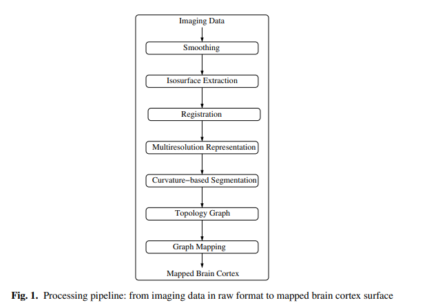
Our brain mapping approach is based on a pipeline of automated steps. Figure 1 illustrates the sequence of individual processing steps.

The input for our processing pipeline is discrete imaging data in some raw format. Typically, imaging techniques produce stacks of aligned images. If the images are not aligned, appropriate alignment tools must be applied [25]. Volumetric reconstruction results in a volume data set, a trivariate scalar field.

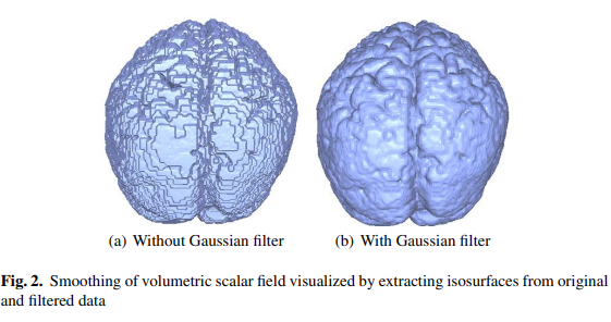
Depending on the used imaging technique, a scanned data set may contain more or less noise. We mainly operate on fMRI data sets, thus having to deal with significant noise levels. We use a three-dimensional discrete Gaussian smoothing filter, which eliminates high-frequency noise without affecting visibly the characteristics of the three-dimensional scalar field. The size of the Gaussian filter must be small. We use a $3 \times 3 \times 3$ mask locally to smooth every value of a rectilinear, regular hexahedral mesh. Figure 2 shows the effect of the smoothing filter applied to a three-dimensional scalar field by extracting isosurfaces from the original and filtered data set.

After this preprocessing step, we extract the geometry of the brain cortex from the volume data. The boundary of the brain cortex is obtained via an isosurface extraction step, as described in Sect. 4. If desired, isosurface extraction can be controlled and supervised in a fashion intuitive to neuroscientists.

Once the geometry of the brain cortices is available for both atlas brain and a user brain, the two surfaces can be registered. Since our brain mapping approach is feature-based, we perform the registration step by a simple and fast rigid body transformation. For an overview and a comparison of rigid body transformation methods, we refer to [6].

统计代写|数据可视化代写Data visualization代考|DTSA5304

数据可视化代考

统计代写|数据可视化代写Data visualization代考|Related Work

最初的脑映射方法使用刚性模型和空间分布。在[26]中,立体定向图谱以正交网格系统表示,该网格系统被重新缩放到患者的大脑,假设特定地标的一对一对应。在$[2,5,11]$中讨论了使用弹性变换的类似方法。在同一物种的不同个体之间,大脑形状和几何形状的差异具有显著的程度。静态刚性模型不足以恰当地描述这种主体间的变化。

通过提供可弹性变形以匹配患者大脑的地图集,引入可变形模型作为处理大脑表面高度复杂性的一种手段。可变形模型使用蛇形[20]、b样条曲面[24]或其他基于曲面的变形算法[8,9]。特征匹配是通过最小化代价函数来实现的,代价函数是基于由测量变形和相似度的总和定义的误差度量。成本函数的定义至关重要。一些方法依赖于用户引导的主沟分割[4,27,29],而其他方法则自动生成表面的结构描述。

如[21]所述,水平集方法被广泛用于凸形状。这些方法以局部能量最小化为基础,实现了在已知曲面信息很少的情况下的形状识别。初始化必须在接近表面边界的地方完成,并且需要交互式种子放置。已经提出了几种方法来执行自动播种过程并适应外部传播力[1],但仍然可能遗漏小特征。使用皮层模型的多分辨率表示,患者和图谱网格通过[16]中描述的方法逐步匹配。在给定的分辨率下,根据大小对折叠进行注释。决议的选择至关重要。不能保证相同的特征在不同的大脑中以相同的分辨率呈现。

存在许多其他自动方法,包括使用活动带[10,13]、图形表示[3,22]和区域生长[18]的技术。[28]提供了一项调查。尽管一些方法提供了良好的结果,但皮质表面的高度非凸形状,加上主体间的可变性和特征尺寸的可变性,会导致问题,并可能在没有用户干预的情况下阻止正确的特征识别/分割和映射。

我们的方法是一种自动化的方法,可以处理高度非凸的形状,因为我们将大脑分割成皮质区域,并且具有特征大小和主体间的可变性,因为它是基于离散曲率行为。此外,等值面提取、曲面分割和拓扑图嵌入到图形系统中,支持视觉理解。

统计代写|数据可视化代写Data visualization代考|Brain Mapping

我们的大脑映射方法是基于自动化步骤的流水线。图1说明了各个处理步骤的顺序。

我们处理管道的输入是一些原始格式的离散成像数据。通常,成像技术产生一堆对齐的图像。如果图像没有对齐,则必须应用适当的对齐工具[25]。体积重建的结果是一个体积数据集,一个三元标量场。

根据所使用的成像技术,扫描的数据集可能包含或多或少的噪声。我们主要对fMRI数据集进行操作,因此必须处理显著的噪声水平。我们使用三维离散高斯平滑滤波器,在不明显影响三维标量场特性的情况下消除高频噪声。高斯滤波器的大小必须很小。我们使用$3 \ × 3 \ × 3$局部掩码来平滑一个直线型、正六面体网格的每个值。图2显示了通过从原始和过滤后的数据集中提取等值面,将平滑滤波器应用于三维标量场的效果。

在此预处理步骤之后,我们从体积数据中提取大脑皮层的几何形状。大脑皮层的边界是通过等值面提取步骤获得的,如第4节所述。如果需要,等值面提取可以以神经科学家直观的方式进行控制和监督。

一旦图谱脑和用户脑的大脑皮层的几何形状可用,这两个表面就可以被注册。由于我们的脑映射方法是基于特征的,我们通过一个简单而快速的刚体转换来执行注册步骤

统计代写|数据可视化代写Data visualization代考 请认准statistics-lab™

统计代写请认准statistics-lab™. statistics-lab™为您的留学生涯保驾护航。

金融工程代写

金融工程是使用数学技术来解决金融问题。金融工程使用计算机科学、统计学、经济学和应用数学领域的工具和知识来解决当前的金融问题,以及设计新的和创新的金融产品。

非参数统计代写

非参数统计指的是一种统计方法,其中不假设数据来自于由少数参数决定的规定模型;这种模型的例子包括正态分布模型和线性回归模型。

广义线性模型代考

广义线性模型(GLM)归属统计学领域,是一种应用灵活的线性回归模型。该模型允许因变量的偏差分布有除了正态分布之外的其它分布。

术语 广义线性模型(GLM)通常是指给定连续和/或分类预测因素的连续响应变量的常规线性回归模型。它包括多元线性回归,以及方差分析和方差分析(仅含固定效应)。

有限元方法代写

有限元方法(FEM)是一种流行的方法,用于数值解决工程和数学建模中出现的微分方程。典型的问题领域包括结构分析、传热、流体流动、质量运输和电磁势等传统领域。

有限元是一种通用的数值方法,用于解决两个或三个空间变量的偏微分方程(即一些边界值问题)。为了解决一个问题,有限元将一个大系统细分为更小、更简单的部分,称为有限元。这是通过在空间维度上的特定空间离散化来实现的,它是通过构建对象的网格来实现的:用于求解的数值域,它有有限数量的点。边界值问题的有限元方法表述最终导致一个代数方程组。该方法在域上对未知函数进行逼近。[1] 然后将模拟这些有限元的简单方程组合成一个更大的方程系统,以模拟整个问题。然后,有限元通过变化微积分使相关的误差函数最小化来逼近一个解决方案。

tatistics-lab作为专业的留学生服务机构,多年来已为美国、英国、加拿大、澳洲等留学热门地的学生提供专业的学术服务,包括但不限于Essay代写,Assignment代写,Dissertation代写,Report代写,小组作业代写,Proposal代写,Paper代写,Presentation代写,计算机作业代写,论文修改和润色,网课代做,exam代考等等。写作范围涵盖高中,本科,研究生等海外留学全阶段,辐射金融,经济学,会计学,审计学,管理学等全球99%专业科目。写作团队既有专业英语母语作者,也有海外名校硕博留学生,每位写作老师都拥有过硬的语言能力,专业的学科背景和学术写作经验。我们承诺100%原创,100%专业,100%准时,100%满意。

随机分析代写


随机微积分是数学的一个分支,对随机过程进行操作。它允许为随机过程的积分定义一个关于随机过程的一致的积分理论。这个领域是由日本数学家伊藤清在第二次世界大战期间创建并开始的。

时间序列分析代写

随机过程,是依赖于参数的一组随机变量的全体,参数通常是时间。 随机变量是随机现象的数量表现,其时间序列是一组按照时间发生先后顺序进行排列的数据点序列。通常一组时间序列的时间间隔为一恒定值(如1秒,5分钟,12小时,7天,1年),因此时间序列可以作为离散时间数据进行分析处理。研究时间序列数据的意义在于现实中,往往需要研究某个事物其随时间发展变化的规律。这就需要通过研究该事物过去发展的历史记录,以得到其自身发展的规律。

回归分析代写

多元回归分析渐进(Multiple Regression Analysis Asymptotics)属于计量经济学领域,主要是一种数学上的统计分析方法,可以分析复杂情况下各影响因素的数学关系,在自然科学、社会和经济学等多个领域内应用广泛。

MATLAB代写

MATLAB 是一种用于技术计算的高性能语言。它将计算、可视化和编程集成在一个易于使用的环境中,其中问题和解决方案以熟悉的数学符号表示。典型用途包括:数学和计算算法开发建模、仿真和原型制作数据分析、探索和可视化科学和工程图形应用程序开发,包括图形用户界面构建MATLAB 是一个交互式系统,其基本数据元素是一个不需要维度的数组。这使您可以解决许多技术计算问题,尤其是那些具有矩阵和向量公式的问题,而只需用 C 或 Fortran 等标量非交互式语言编写程序所需的时间的一小部分。MATLAB 名称代表矩阵实验室。MATLAB 最初的编写目的是提供对由 LINPACK 和 EISPACK 项目开发的矩阵软件的轻松访问,这两个项目共同代表了矩阵计算软件的最新技术。MATLAB 经过多年的发展,得到了许多用户的投入。在大学环境中,它是数学、工程和科学入门和高级课程的标准教学工具。在工业领域,MATLAB 是高效研究、开发和分析的首选工具。MATLAB 具有一系列称为工具箱的特定于应用程序的解决方案。对于大多数 MATLAB 用户来说非常重要,工具箱允许您学习应用专业技术。工具箱是 MATLAB 函数(M 文件)的综合集合,可扩展 MATLAB 环境以解决特定类别的问题。可用工具箱的领域包括信号处理、控制系统、神经网络、模糊逻辑、小波、仿真等。

R语言代写问卷设计与分析代写
PYTHON代写回归分析与线性模型代写
MATLAB代写方差分析与试验设计代写
STATA代写机器学习/统计学习代写
SPSS代写计量经济学代写
EVIEWS代写时间序列分析代写
EXCEL代写深度学习代写
SQL代写各种数据建模与可视化代写

统计代写|数据可视化代写Data visualization代考|CSE512

如果你也在 怎样代写数据可视化Data visualization这个学科遇到相关的难题,请随时右上角联系我们的24/7代写客服。

数据可视化是将信息转化为视觉背景的做法,如地图或图表,使数据更容易被人脑理解并从中获得洞察力。数据可视化的主要目标是使其更容易在大型数据集中识别模式、趋势和异常值。

statistics-lab™ 为您的留学生涯保驾护航 在代写数据可视化Data visualization方面已经树立了自己的口碑, 保证靠谱, 高质且原创的统计Statistics代写服务。我们的专家在代写数据可视化Data visualization代写方面经验极为丰富,各种代写数据可视化Data visualization相关的作业也就用不着说。

我们提供的数据可视化Data visualization及其相关学科的代写,服务范围广, 其中包括但不限于:

  • Statistical Inference 统计推断
  • Statistical Computing 统计计算
  • Advanced Probability Theory 高等概率论
  • Advanced Mathematical Statistics 高等数理统计学
  • (Generalized) Linear Models 广义线性模型
  • Statistical Machine Learning 统计机器学习
  • Longitudinal Data Analysis 纵向数据分析
  • Foundations of Data Science 数据科学基础
统计代写|数据可视化代写Data visualization代考|INFS6023

统计代写|数据可视化代写Data visualization代考|Williams’ Convexification Framework

In his seminal paper [41] on techniques for computing visibility orderings for meshes, Williams discusses the problem of handling non-convex meshes (Sect. 9). (Also related is Sect. 8, which contains a discussion of cycles and the use of Delaunay triangulations.) After explaining some challenges of using his visibility sorting algorithm on non-convex meshes, Williams says:
“Therefore, an important area of research is to find ways to convert nonconvex meshes into convex meshes, so that the regular MPVO algorithm can be used.”
Williams proposes two solution approaches to the problem; each relies on “treating the voids and cavities as ‘imaginary’ cells in the mesh.” Basically, he proposes that such non-convex regions could be either triangulated or decomposed into convex pieces, and their parts marked as imaginary cells for the purpose of rendering. Implementing this “simple idea” is actually not easy. In fact, after discussing this general approach, Williams talks about some of the challenges, and finishes the section with the following remark:
“The implementation of the preprocessing methods, described in this section, for converting a non-convex mesh into a convex mesh could take a very significant amount of time; they are by no means trivial. The implementation of a 3D conformed Delaunay triangulation is still a research question at this time.”
In fact, Williams does not provide an implementation of any of the two proposed convexification algorithms. Instead, he developed a variant of MPVO that works on non-convex meshes at the expense of not being guaranteed to generate correct visibility orders.

The first convexification technique that Williams proposes is based on triangulating the data using a conforming Delaunay triangulation. The idea here is to keep adding more points to the dataset until the original triangulation becomes a Delaunay triangulation. This is discussed in more details in the next section.

The second technique Williams sketches is based on the idea of applying a decomposition algorithm to each of the non-convex polyhedra that constitute the set $\mathrm{CH}(\mathrm{S}) \backslash S$, which is the set difference between the convex hull of the mesh and the mesh itself. In general, $\mathrm{CH}(\mathrm{S}) \backslash S$ is a union of highly non-convex polyhedra of complex topology. Each connected component of $\mathrm{CH}(\mathrm{S}) \backslash S$ is a non-convex polyhedron that can be decomposed into convex polyhedra (e.g., tetrahedra) using, for example, the algorithm of Chazelle and Palios [10], which adds certain new vertices (Steiner points), whose number depends on the number of “reflex” edges of the polyhedron. In general, non-convex polyhedra require the addition of Steiner points in order to decompose them; in fact, it is NP-complete to decide if a polyhedron can be tetrahedralized without the addition of Steiner points.

统计代写|数据可视化代写Data visualization代考|Issues

Achieving Peter Williams’s vision of a simple convexification algorithm is much harder than it appears at first. The problem is peculiar since we start with an existing 3D mesh (likely to be a tetrahedralization) that contains not only vertices, edges, and triangles, but also volumetric cells, which need to be respected. Furthermore, the mesh is not guaranteed to respect global geometric criteria (e.g., of being Delaunay). Most techniques need to modify the original mesh in some way. The goal is to “disturb” it as little as possible, preserving most of its original properties.
In particular, several issues need to be considered:
Preserving Acyclicity. Even if the original mesh has no cycles, the convexification process can potentially cause the resulting convex mesh to contain cycles. Certain techniques, such as constructing a conforming Delaunay tetrahedralization, are guaranteed to generate a cycle-free mesh. Ideally, the convexification procedure will not create new cycles in the mesh.

Output Size. For the convexification technique to be useful the number of cells added by the algorithm needs to be kept as small as possible. Ideally, there is a provable bound on the number of cells as well as experimental evidence that for typical input meshes, the size of the output mesh is not much larger than the input mesh (i.e., the set of additional cells is small).

Computational and Memory Complexity. Other important factors are the processing time and the amount of memory used in the algorithm. In order to be practical on the meshes that arise in computational experiments (having on the order of several thousand to a few million cells), convexification algorithms must run in near-linear time, in practice.

Boundary and Interior Preservation. Ideally, the convexification procedure adds cells only “outside” of the original mesh. Furthermore, the newly created cells should exactly match the original boundary of the mesh. In general, this is not feasible without subdividing or modifying the original cells in some way (e.g., to break cycles, or to add extra geometry in order to respect the Delaunay empty-circumsphere condition). Some techniques will only need to modify the cells that are at or near the original boundary while others might need to perform more global modifications that go all the way “inside” the original mesh. One needs to be careful when making such modifications because of issues related to interpolating the original data values in the mesh. Otherwise, the visualization algorithm may generate incorrect pictures leading to wrong comprehension.

Robustness and Degeneracy Handling. It is very important for the convexification algorithms to handle real data. Large scientific datasets often use floating-point precision for specifying vertices, and are likely to have a number of degeneracies. For instance, these datasets are likely to have many vertices (sample points) that are coplanar, or that lie on a common cylinder or sphere, etc., since the underlying physical model may have such features.

统计代写|数据可视化代写Data visualization代考|CSE512

数据可视化代考

统计代写|数据可视化代写Data visualization代考|Williams’ Convexification Framework

在他关于计算网格可见性排序技术的开创性论文[41]中,Williams讨论了处理非凸网格的问题(章节9)。(同样相关的章节8包含了对循环和Delaunay三角剖分的讨论。)在解释了在非凸网格上使用他的可见性排序算法的一些挑战之后,Williams说:
“因此,一个重要的研究领域是找到将非凸网格转换为凸网格的方法,以便可以使用常规的MPVO算法。”
威廉姆斯提出了两种解决问题的方法;每一种方法都依赖于“将空洞和空腔视为网格中的‘想象’细胞”。基本上,他提出可以将这些非凸区域三角化或分解为凸块,并将其部分标记为假想单元,以便渲染。实现这个“简单的想法”其实并不容易。事实上,在讨论了这种一般方法之后,Williams谈到了一些挑战,并以以下评论结束了这一节:
“本节中描述的将非凸网格转换为凸网格的预处理方法的实现可能需要非常多的时间;它们绝不是微不足道的。目前,实现三维符合Delaunay三角剖分仍然是一个研究问题。”
事实上,Williams并没有提供任何两种凸化算法的实现。相反,他开发了一种MPVO的变体,可以在非凸网格上工作,但代价是不能保证生成正确的可见性顺序。

Williams提出的第一种凸化技术是基于使用符合的Delaunay三角剖分法对数据进行三角剖分。这里的想法是不断向数据集中添加更多的点,直到原始三角剖分变成Delaunay三角剖分。下一节将对此进行更详细的讨论。

Williams概述的第二种技术是基于将分解算法应用于构成集合$\ mathm {CH}(\ mathm {S}) \反斜杠S$的每个非凸多面体的思想,这是网格的凸壳和网格本身之间的集合差。一般来说,$\ mathm {CH}(\ mathm {S}) \反斜杠S$是复拓扑的高度非凸多面体的并。$\ mathm {CH}(\ mathm {S}) \反斜线S$的每个连通成分都是一个非凸多面体,可以使用例如Chazelle和Palios[10]的算法分解为凸多面体(例如,四面体),该算法添加了某些新顶点(斯坦纳点),其数量取决于多面体的“反射”边的数量。一般来说,非凸多面体需要添加斯坦纳点来分解它们;事实上,在不加施泰纳点的情况下判定多面体是否可以四面体是np完全的。

统计代写|数据可视化代写Data visualization代考|Issues

实现彼得·威廉姆斯关于一个简单的凸化算法的设想比乍看起来要困难得多。这个问题很特殊,因为我们从一个现有的3D网格(可能是一个四面体)开始,它不仅包含顶点、边和三角形,还包含需要尊重的体积单元。此外,网格不能保证遵守全局几何标准(例如,Delaunay)。大多数技术都需要以某种方式修改原始网格。我们的目标是尽可能少地“干扰”它,保留它的大部分原始属性。
特别是有几个问题需要考虑:
保留Acyclicity。即使原始网格没有循环,凸化过程也可能导致最终的凸网格包含循环。某些技术,如构造符合的德劳内四面体化,保证生成无循环网格。理想情况下,凸化过程不会在网格中产生新的循环。

输出的大小。为了使凸化技术有效,算法添加的单元数必须尽可能小。理想情况下,对于典型的输入网格,输出网格的大小不会比输入网格大多少(即,额外的单元集很小),并且有一个可证明的细胞数量界限。

计算和内存复杂性。其他重要的因素是处理时间和算法中使用的内存量。为了在计算实验中出现的网格(有几千到几百万个单元)上实用,在实践中,凸化算法必须在接近线性的时间内运行。

边界和内部保存。理想情况下,凸化过程只在原始网格的“外部”添加细胞。此外,新创建的单元应该完全匹配网格的原始边界。一般来说,如果不以某种方式细分或修改原始细胞,这是不可行的(例如,打破循环,或添加额外的几何形状,以尊重德劳内空环条件)。一些技术将只需要修改在原始边界或附近的单元格,而其他技术可能需要执行更多的全局修改,一直“进入”原始网格。在进行此类修改时需要小心,因为与网格中原始数据值的插值相关的问题。否则,可视化算法可能会生成错误的图片,导致错误的理解。

鲁棒性和退化处理。对于凸化算法来说,处理真实数据是非常重要的。大型科学数据集通常使用浮点精度来指定顶点,并且可能有许多退化。例如,这些数据集可能有许多共面顶点(样本点),或者位于共同的圆柱体或球体上,等等,因为底层物理模型可能具有这些特征。

统计代写|数据可视化代写Data visualization代考 请认准statistics-lab™

统计代写请认准statistics-lab™. statistics-lab™为您的留学生涯保驾护航。

金融工程代写

金融工程是使用数学技术来解决金融问题。金融工程使用计算机科学、统计学、经济学和应用数学领域的工具和知识来解决当前的金融问题,以及设计新的和创新的金融产品。

非参数统计代写

非参数统计指的是一种统计方法,其中不假设数据来自于由少数参数决定的规定模型;这种模型的例子包括正态分布模型和线性回归模型。

广义线性模型代考

广义线性模型(GLM)归属统计学领域,是一种应用灵活的线性回归模型。该模型允许因变量的偏差分布有除了正态分布之外的其它分布。

术语 广义线性模型(GLM)通常是指给定连续和/或分类预测因素的连续响应变量的常规线性回归模型。它包括多元线性回归,以及方差分析和方差分析(仅含固定效应)。

有限元方法代写

有限元方法(FEM)是一种流行的方法,用于数值解决工程和数学建模中出现的微分方程。典型的问题领域包括结构分析、传热、流体流动、质量运输和电磁势等传统领域。

有限元是一种通用的数值方法,用于解决两个或三个空间变量的偏微分方程(即一些边界值问题)。为了解决一个问题,有限元将一个大系统细分为更小、更简单的部分,称为有限元。这是通过在空间维度上的特定空间离散化来实现的,它是通过构建对象的网格来实现的:用于求解的数值域,它有有限数量的点。边界值问题的有限元方法表述最终导致一个代数方程组。该方法在域上对未知函数进行逼近。[1] 然后将模拟这些有限元的简单方程组合成一个更大的方程系统,以模拟整个问题。然后,有限元通过变化微积分使相关的误差函数最小化来逼近一个解决方案。

tatistics-lab作为专业的留学生服务机构,多年来已为美国、英国、加拿大、澳洲等留学热门地的学生提供专业的学术服务,包括但不限于Essay代写,Assignment代写,Dissertation代写,Report代写,小组作业代写,Proposal代写,Paper代写,Presentation代写,计算机作业代写,论文修改和润色,网课代做,exam代考等等。写作范围涵盖高中,本科,研究生等海外留学全阶段,辐射金融,经济学,会计学,审计学,管理学等全球99%专业科目。写作团队既有专业英语母语作者,也有海外名校硕博留学生,每位写作老师都拥有过硬的语言能力,专业的学科背景和学术写作经验。我们承诺100%原创,100%专业,100%准时,100%满意。

随机分析代写


随机微积分是数学的一个分支,对随机过程进行操作。它允许为随机过程的积分定义一个关于随机过程的一致的积分理论。这个领域是由日本数学家伊藤清在第二次世界大战期间创建并开始的。

时间序列分析代写

随机过程,是依赖于参数的一组随机变量的全体,参数通常是时间。 随机变量是随机现象的数量表现,其时间序列是一组按照时间发生先后顺序进行排列的数据点序列。通常一组时间序列的时间间隔为一恒定值(如1秒,5分钟,12小时,7天,1年),因此时间序列可以作为离散时间数据进行分析处理。研究时间序列数据的意义在于现实中,往往需要研究某个事物其随时间发展变化的规律。这就需要通过研究该事物过去发展的历史记录,以得到其自身发展的规律。

回归分析代写

多元回归分析渐进(Multiple Regression Analysis Asymptotics)属于计量经济学领域,主要是一种数学上的统计分析方法,可以分析复杂情况下各影响因素的数学关系,在自然科学、社会和经济学等多个领域内应用广泛。

MATLAB代写

MATLAB 是一种用于技术计算的高性能语言。它将计算、可视化和编程集成在一个易于使用的环境中,其中问题和解决方案以熟悉的数学符号表示。典型用途包括:数学和计算算法开发建模、仿真和原型制作数据分析、探索和可视化科学和工程图形应用程序开发,包括图形用户界面构建MATLAB 是一个交互式系统,其基本数据元素是一个不需要维度的数组。这使您可以解决许多技术计算问题,尤其是那些具有矩阵和向量公式的问题,而只需用 C 或 Fortran 等标量非交互式语言编写程序所需的时间的一小部分。MATLAB 名称代表矩阵实验室。MATLAB 最初的编写目的是提供对由 LINPACK 和 EISPACK 项目开发的矩阵软件的轻松访问,这两个项目共同代表了矩阵计算软件的最新技术。MATLAB 经过多年的发展,得到了许多用户的投入。在大学环境中,它是数学、工程和科学入门和高级课程的标准教学工具。在工业领域,MATLAB 是高效研究、开发和分析的首选工具。MATLAB 具有一系列称为工具箱的特定于应用程序的解决方案。对于大多数 MATLAB 用户来说非常重要,工具箱允许您学习应用专业技术。工具箱是 MATLAB 函数(M 文件)的综合集合,可扩展 MATLAB 环境以解决特定类别的问题。可用工具箱的领域包括信号处理、控制系统、神经网络、模糊逻辑、小波、仿真等。

R语言代写问卷设计与分析代写
PYTHON代写回归分析与线性模型代写
MATLAB代写方差分析与试验设计代写
STATA代写机器学习/统计学习代写
SPSS代写计量经济学代写
EVIEWS代写时间序列分析代写
EXCEL代写深度学习代写
SQL代写各种数据建模与可视化代写

统计代写|数据可视化代写Data visualization代考|INFS6023

如果你也在 怎样代写数据可视化Data visualization这个学科遇到相关的难题,请随时右上角联系我们的24/7代写客服。

数据可视化是将信息转化为视觉背景的做法,如地图或图表,使数据更容易被人脑理解并从中获得洞察力。数据可视化的主要目标是使其更容易在大型数据集中识别模式、趋势和异常值。

statistics-lab™ 为您的留学生涯保驾护航 在代写数据可视化Data visualization方面已经树立了自己的口碑, 保证靠谱, 高质且原创的统计Statistics代写服务。我们的专家在代写数据可视化Data visualization代写方面经验极为丰富,各种代写数据可视化Data visualization相关的作业也就用不着说。

我们提供的数据可视化Data visualization及其相关学科的代写,服务范围广, 其中包括但不限于:

  • Statistical Inference 统计推断
  • Statistical Computing 统计计算
  • Advanced Probability Theory 高等概率论
  • Advanced Mathematical Statistics 高等数理统计学
  • (Generalized) Linear Models 广义线性模型
  • Statistical Machine Learning 统计机器学习
  • Longitudinal Data Analysis 纵向数据分析
  • Foundations of Data Science 数据科学基础
统计代写|数据可视化代写Data visualization代考|INFS6023

统计代写|数据可视化代写Data visualization代考|Fitting Quadratic Curves

Given a set of function values $f_0, f_1 \ldots f_n$ at positions $x_0, x_1 \ldots x_n$, we create a quadratic function that passes through the end points and approximates the remaining data values.

The quadratic function $C(t)$ we use to approximate the function values along an edge is defined as
$$
C(t)=\sum_{i=0}^2 c_i B_i^2(t)
$$
The quadratic Bernstein polynomial $B_i^2(t)$ is defined as
$$
B_i^2(t)=\frac{2 !}{(2-i) ! i !}(1-u)^{2-i} u^i
$$

First we parameterize the data by assigning parameter values $t_0, t_1 \ldots t_n$ in the interval $[0,1]$ to the positions $x_0, x_1 \ldots x_n$. Parameter values are defined with a chordlength parameterization as
$$
t_i=\frac{x_i-x_0}{x_n-x_0}
$$
Next, we solve a least-squares approximation problem to determine the coefficients $c_i$ of $C(t)$. The resulting overdetermined system of linear equations is
$$
\left[\begin{array}{ccc}
\left(1-t_0\right)^2 & 2\left(1-t_0\right) t_0 & t_0^2 \
\left(1-t_1\right)^2 & 2\left(1-t_1\right) t_1 & t_1^2 \
\vdots & \vdots & \vdots \
\left(1-t_n\right)^2 & 2\left(1-t_n\right) t_n & t_n^2
\end{array}\right]\left[\begin{array}{c}
c_0 \
c_1 \
c_2
\end{array}\right]=\left[\begin{array}{c}
f_0 \
f_1 \
\vdots \
f_n
\end{array}\right] .
$$
Constraining $C(t)$, so that it interpolates the endpoint values, i.e. $C(0)=f_0$ and $C(1)=f_n$, leads to the system
$$
\begin{gathered}
{\left[\begin{array}{c}
2\left(1-t_1\right) t_1 \
2\left(1-t_2\right) t_2 \
\vdots \
2\left(1-t_{n-1}\right) t_{n-1}
\end{array}\right]\left[c_1\right]=} \
{\left[\begin{array}{c}
f_1-f_0\left(1-t_1\right)^2-f_n t_1^2 \
f_2-f_0\left(1-t_2\right)^2-f_n t_2{ }^2 \
\vdots \
f_{n-1}-f_0\left(1-t_{n-1}\right)^2-f_n t_{n-1}{ }^2
\end{array}\right]}
\end{gathered}
$$
for the one degree of freedom $c_1$.

统计代写|数据可视化代写Data visualization代考|Approximating a Dataset

A quadratic approximation of a dataset is created by approximating the data values along each edge in the tetrahedral mesh with a quadratic function as described in Sect. 4.1. Each linear tetrahedron becomes a quadratic tetrahedron. The resulting approximation is $C^1$-continuous within a tetrahedron and $C^0$-continuous on shared faces and edges. The approximation error $e_a$ for a tetrahedron $T$ is the maximum difference between the quadratic approximation over $T$ and all original data values associated with points inside and on $T$ ‘ $s$ boundary.

In tetrahedral meshes created by longest-edge bisection, each edge $E$ in the mesh, except for the edges at the finest level of the mesh, is the split edge of a diamond $D$, see [5], and is associated with a split vertex $S V$. The computed coefficient $c_1$ for the edge $E$ is stored with the split vertex $S V$. The edges used for computing the quadratic representation can be enumerated by recursively traversing the tetrahedral mesh and examining the refinement edges. This process is illustrated for the $2 \mathrm{D}$ case in Fig. 2 . Since quadratic tetrahedra have three coefficients along each edge, the leaf level of a mesh with quadratic tetrahedra is one level higher in the mesh than the leaf level for linear tetrahedra, see Fig. 3.

In summary, we construct a quadratic approximation of a volume data set as follows:

  1. For each edge of the mesh hierarchy, approximate the data values along the edge with a quadratic function that passes through the endpoints.
  2. For each tetrahedron in the hierarchy, construct a quadratic tetrahedron from the six quadratic functions along its edges.
  3. Compute the approximation error $e_a$ for each tetrahedron.
统计代写|数据可视化代写Data visualization代考|INFS6023

数据可视化代考

统计代写|数据可视化代写Data visualization代考|Fitting Quadratic Curves

给定一组位于$x_0, x_1 \ldots x_n$位置的函数值$f_0, f_1 \ldots f_n$,我们创建一个二次函数,该函数通过端点并近似其余的数据值。

我们用来沿一条边近似函数值的二次函数$C(t)$定义为
$$
C(t)=\sum_{i=0}^2 c_i B_i^2(t)
$$
二次Bernstein多项式$B_i^2(t)$定义为
$$
B_i^2(t)=\frac{2 !}{(2-i) ! i !}(1-u)^{2-i} u^i
$$

首先,我们通过将区间$[0,1]$中的参数值$t_0, t_1 \ldots t_n$分配给位置$x_0, x_1 \ldots x_n$来参数化数据。参数值用弦长参数化定义为
$$
t_i=\frac{x_i-x_0}{x_n-x_0}
$$
接下来,我们解决一个最小二乘近似问题来确定$C(t)$的系数$c_i$。由此得到的过定线性方程组为
$$
\left[\begin{array}{ccc}
\left(1-t_0\right)^2 & 2\left(1-t_0\right) t_0 & t_0^2 \
\left(1-t_1\right)^2 & 2\left(1-t_1\right) t_1 & t_1^2 \
\vdots & \vdots & \vdots \
\left(1-t_n\right)^2 & 2\left(1-t_n\right) t_n & t_n^2
\end{array}\right]\left[\begin{array}{c}
c_0 \
c_1 \
c_2
\end{array}\right]=\left[\begin{array}{c}
f_0 \
f_1 \
\vdots \
f_n
\end{array}\right] .
$$
约束$C(t)$,使其内插端点值,即$C(0)=f_0$和$C(1)=f_n$,导致系统
$$
\begin{gathered}
{\left[\begin{array}{c}
2\left(1-t_1\right) t_1 \
2\left(1-t_2\right) t_2 \
\vdots \
2\left(1-t_{n-1}\right) t_{n-1}
\end{array}\right]\left[c_1\right]=} \
{\left[\begin{array}{c}
f_1-f_0\left(1-t_1\right)^2-f_n t_1^2 \
f_2-f_0\left(1-t_2\right)^2-f_n t_2{ }^2 \
\vdots \
f_{n-1}-f_0\left(1-t_{n-1}\right)^2-f_n t_{n-1}{ }^2
\end{array}\right]}
\end{gathered}
$$
对于一个自由度$c_1$。

统计代写|数据可视化代写Data visualization代考|Approximating a Dataset

数据集的二次逼近是通过使用第4.1节中描述的二次函数近似四面体网格中每条边的数据值来创建的。每个线性四面体变成一个二次四面体。得到的近似是$C^1$ -在四面体内连续,$C^0$ -在共享的面和边上连续。四面体$T$的近似误差$e_a$是$T$上的二次近似与与$T$ ‘ $s$边界内和上的点相关的所有原始数据值之间的最大差值。

在由最长边缘对分创建的四面体网格中,除了网格最细层次的边缘外,网格中的每个边缘$E$都是菱形的分裂边缘$D$,参见[5],并且与分裂顶点$S V$相关联。计算出的边$E$的系数$c_1$与分裂的顶点$S V$一起存储。用于计算二次表示的边可以通过递归遍历四面体网格并检查细化边来枚举。这一过程在图2中对$2 \mathrm{D}$的情况进行了说明。由于二次四面体在每条边有三个系数,因此二次四面体网格的叶位比线性四面体网格的叶位高一级,如图3所示。

综上所述,我们构造了一个体积数据集的二次逼近:

对于网格层次结构的每个边缘,使用经过端点的二次函数沿边缘近似计算数据值。

对于层次结构中的每个四面体,从沿其边缘的六个二次函数构造一个二次四面体。

计算每个四面体的近似误差$e_a$。

统计代写|数据可视化代写Data visualization代考 请认准statistics-lab™

统计代写请认准statistics-lab™. statistics-lab™为您的留学生涯保驾护航。

金融工程代写

金融工程是使用数学技术来解决金融问题。金融工程使用计算机科学、统计学、经济学和应用数学领域的工具和知识来解决当前的金融问题,以及设计新的和创新的金融产品。

非参数统计代写

非参数统计指的是一种统计方法,其中不假设数据来自于由少数参数决定的规定模型;这种模型的例子包括正态分布模型和线性回归模型。

广义线性模型代考

广义线性模型(GLM)归属统计学领域,是一种应用灵活的线性回归模型。该模型允许因变量的偏差分布有除了正态分布之外的其它分布。

术语 广义线性模型(GLM)通常是指给定连续和/或分类预测因素的连续响应变量的常规线性回归模型。它包括多元线性回归,以及方差分析和方差分析(仅含固定效应)。

有限元方法代写

有限元方法(FEM)是一种流行的方法,用于数值解决工程和数学建模中出现的微分方程。典型的问题领域包括结构分析、传热、流体流动、质量运输和电磁势等传统领域。

有限元是一种通用的数值方法,用于解决两个或三个空间变量的偏微分方程(即一些边界值问题)。为了解决一个问题,有限元将一个大系统细分为更小、更简单的部分,称为有限元。这是通过在空间维度上的特定空间离散化来实现的,它是通过构建对象的网格来实现的:用于求解的数值域,它有有限数量的点。边界值问题的有限元方法表述最终导致一个代数方程组。该方法在域上对未知函数进行逼近。[1] 然后将模拟这些有限元的简单方程组合成一个更大的方程系统,以模拟整个问题。然后,有限元通过变化微积分使相关的误差函数最小化来逼近一个解决方案。

tatistics-lab作为专业的留学生服务机构,多年来已为美国、英国、加拿大、澳洲等留学热门地的学生提供专业的学术服务,包括但不限于Essay代写,Assignment代写,Dissertation代写,Report代写,小组作业代写,Proposal代写,Paper代写,Presentation代写,计算机作业代写,论文修改和润色,网课代做,exam代考等等。写作范围涵盖高中,本科,研究生等海外留学全阶段,辐射金融,经济学,会计学,审计学,管理学等全球99%专业科目。写作团队既有专业英语母语作者,也有海外名校硕博留学生,每位写作老师都拥有过硬的语言能力,专业的学科背景和学术写作经验。我们承诺100%原创,100%专业,100%准时,100%满意。

随机分析代写


随机微积分是数学的一个分支,对随机过程进行操作。它允许为随机过程的积分定义一个关于随机过程的一致的积分理论。这个领域是由日本数学家伊藤清在第二次世界大战期间创建并开始的。

时间序列分析代写

随机过程,是依赖于参数的一组随机变量的全体,参数通常是时间。 随机变量是随机现象的数量表现,其时间序列是一组按照时间发生先后顺序进行排列的数据点序列。通常一组时间序列的时间间隔为一恒定值(如1秒,5分钟,12小时,7天,1年),因此时间序列可以作为离散时间数据进行分析处理。研究时间序列数据的意义在于现实中,往往需要研究某个事物其随时间发展变化的规律。这就需要通过研究该事物过去发展的历史记录,以得到其自身发展的规律。

回归分析代写

多元回归分析渐进(Multiple Regression Analysis Asymptotics)属于计量经济学领域,主要是一种数学上的统计分析方法,可以分析复杂情况下各影响因素的数学关系,在自然科学、社会和经济学等多个领域内应用广泛。

MATLAB代写

MATLAB 是一种用于技术计算的高性能语言。它将计算、可视化和编程集成在一个易于使用的环境中,其中问题和解决方案以熟悉的数学符号表示。典型用途包括:数学和计算算法开发建模、仿真和原型制作数据分析、探索和可视化科学和工程图形应用程序开发,包括图形用户界面构建MATLAB 是一个交互式系统,其基本数据元素是一个不需要维度的数组。这使您可以解决许多技术计算问题,尤其是那些具有矩阵和向量公式的问题,而只需用 C 或 Fortran 等标量非交互式语言编写程序所需的时间的一小部分。MATLAB 名称代表矩阵实验室。MATLAB 最初的编写目的是提供对由 LINPACK 和 EISPACK 项目开发的矩阵软件的轻松访问,这两个项目共同代表了矩阵计算软件的最新技术。MATLAB 经过多年的发展,得到了许多用户的投入。在大学环境中,它是数学、工程和科学入门和高级课程的标准教学工具。在工业领域,MATLAB 是高效研究、开发和分析的首选工具。MATLAB 具有一系列称为工具箱的特定于应用程序的解决方案。对于大多数 MATLAB 用户来说非常重要,工具箱允许您学习应用专业技术。工具箱是 MATLAB 函数(M 文件)的综合集合,可扩展 MATLAB 环境以解决特定类别的问题。可用工具箱的领域包括信号处理、控制系统、神经网络、模糊逻辑、小波、仿真等。

R语言代写问卷设计与分析代写
PYTHON代写回归分析与线性模型代写
MATLAB代写方差分析与试验设计代写
STATA代写机器学习/统计学习代写
SPSS代写计量经济学代写
EVIEWS代写时间序列分析代写
EXCEL代写深度学习代写
SQL代写各种数据建模与可视化代写

统计代写|数据可视化代写Data visualization代考|STAT1100

如果你也在 怎样代写数据可视化Data visualization这个学科遇到相关的难题,请随时右上角联系我们的24/7代写客服。

数据可视化是将信息转化为视觉背景的做法,如地图或图表,使数据更容易被人脑理解并从中获得洞察力。数据可视化的主要目标是使其更容易在大型数据集中识别模式、趋势和异常值。

statistics-lab™ 为您的留学生涯保驾护航 在代写数据可视化Data visualization方面已经树立了自己的口碑, 保证靠谱, 高质且原创的统计Statistics代写服务。我们的专家在代写数据可视化Data visualization代写方面经验极为丰富,各种代写数据可视化Data visualization相关的作业也就用不着说。

我们提供的数据可视化Data visualization及其相关学科的代写,服务范围广, 其中包括但不限于:

  • Statistical Inference 统计推断
  • Statistical Computing 统计计算
  • Advanced Probability Theory 高等概率论
  • Advanced Mathematical Statistics 高等数理统计学
  • (Generalized) Linear Models 广义线性模型
  • Statistical Machine Learning 统计机器学习
  • Longitudinal Data Analysis 纵向数据分析
  • Foundations of Data Science 数据科学基础
统计代写|数据可视化代写Data visualization代考|STAT1100

统计代写|数据可视化代写Data visualization代考|The Laws of Motion

There is, in nature, perhaps nothing older than motion, concerning which the books written by philosophers are neither few nor small; nevertheless I have discovered by experiment some properties of it which are worth knowing and which have not hitherto been either observed or demonstrated.

Galileo’s seventeenth-century observations foreshadow the origins of the cinema, computer-animated films, and-most relevant to this narrativedynamic data graphics. The popularity of modern dynamic data displays can be traced to scientific questions about the nature of human and animal motion. As technology developed, the study of motion and its visualization branched out from a pleasurable pastime to the huge industries of Hollywood and Netflix while also having important scientific applications in aerodynamics (the wind tunnel), medical imaging (blood flow in the heart and brain), and ecology (migratory patterns of animal species) among others

Aristotle’s De Motu Animalium (The Movement of Animals) was the first book setting out the principles of animal locomotion. Nichole Oresme’s 1360 “pipes” diagram (see Figure 2.2) was intended to show some possible mathematical relations between time and distance traveled. Around 1517, Leonardo da Vinci drew detailed anatomical studies of moving cats, horses, and dragons; Galileo later conducted experiments on motion and gravity between 1633 and 1642. However, the modern interest in these questions arose in the late 1800 s when new technologies for recording could provide new insights.
To a physicist, motion is nothing more interesting than a change in position over time. It can be reduced to simple, but elegant, equations giving velocity (the first derivative) and acceleration (the second derivative). A velocity, $v$, of a horse galloping at $45 \mathrm{mph}$ can be reduced to the equation $v=d x / d t=45$. The acceleration, $g$, due to gravity on Earth can very nearly be reduced to a constant, ${ }^2 \mathrm{~g}=9.8 \mathrm{~m} / \mathrm{s}^2$, or $32 \mathrm{ft} / \mathrm{s}^2$.

But to a ballet dancer, the art is in getting all the body parts to do those things in sync with a musical score to tell a wordless story of emotion ${ }^3$ entirely through change in position over time. In data visualization, as in physics and ballet, motion is a manifestation of the relation between time and space, and so the recording and display of motion added time as a fourth dimension to the abstract world of data. We focus here on a few developments that led to the visual depiction, understanding, and explanation of time-changing phenomena.

统计代写|数据可视化代写Data visualization代考|The Horse in Motion

The modern scientific interest in visualizing motion can be traced to some simple yet perplexing questions of the late 1800 s concerning the locomotion of the horse.

  • How exactly do horses’ feet move differently in a walk, a trot, a canter, and a gallop?
  • What is the exact sequence of the four legs in cach gait?
  • How many feet are off the ground at any given time in each gait?
  • Is there any moment, in each gait, when a horse is at least instantaneously suspended in air, with all four feet off the ground?
    In the 1860s to 1870 s, the last question was called “unsupported transit,” and various writers weighed in to argue each side of the controversy. 4

But there were no “data”; no information was available that was sufficiently precise to answer the question convincingly. The motion of a galloping horse was too rapid for either sight or sound to decipher, and even records of the positions of hooves on a specially prepared track could not be used to discern their exact pattern in time and space. In some ways, the armchair discussion on this topic resembled that of what to do about crime in France in the time of Guerry (Chapter 3), or the transmission of cholera in the time of Farr and Snow (Chapter 4).

The debate on horse locomotion was sufficiently intriguing to Leland Stanford (railway baron, governor of California, and a horse breeder) that he hired Eadweard Muybridge [1830-1904], a well-known photographer with a bent for technology, to try to answer the question by photographic means.

Cameras of that time recorded images on glass plates coated with a solution of silver nitrite; each new photograph required a new plate. Over some years, Muybridge devised a system using multiple cameras arranged in a line, with their shutters triggered by parallel strings stretched across the path of a running horse. Figure $9.1$ shows one famous example of twelve successive frames of a horse, “Sally Gardner,” galloping at a Palo Alto track (now the Stanford University campus). Frame 3 plainly shows all four hooves off the ground-settling the question. In other frames, only one foot is in contact with the earth, and the remaining frames provide a detailed account of the different motions of the front and back legs. A visual solution to the question of unsupported transit had been found. Legend has it that Stanford had bet $\$ 25,000$ on the YES side and so was delighted with the outcome.

统计代写|数据可视化代写Data visualization代考|STAT1100

数据可视化代考

统计代写|数据可视化代写Data visualization代考|The Laws of Motion

在自然界中,也许没有比运动更古老的东西了,哲学家们所写的关于运动的书籍既不少又不小;尽管如此,我还是通过实验发现了它的一些特性,这些特性值得了解,而这些特性迄今尚未被观察或证明。

伽利略在 17 世纪的观察预示了电影、计算机动画电影以及与这种叙事动态数据图形最相关的起源。现代动态数据显示的流行可以追溯到关于人类和动物运动本质的科学问题。随着技术的发展,对运动及其可视化的研究从一种令人愉快的消遣活动扩展到好莱坞和 Netflix 的庞大产业,同时在空气动力学(风洞)、医学成像(心脏和大脑中的血流)方面也有重要的科学应用和生态学(动物物种的迁徙模式)等

亚里士多德的 De Motu Animalium(动物运动)是第一本阐述动物运动原理的书。Nichole Oresme 的 1360“管道”图(见图 2.2)旨在显示时间和行进距离之间的一些可能的数学关系。大约在 1517 年,列奥纳多·达·芬奇 (Leonardo da Vinci) 详细绘制了移动的猫、马和龙的解剖学研究;伽利略后来在 1633 年至 1642 年间对运动和重力进行了实验。然而,现代人对这些问题的兴趣出现在 1800 年代后期,当时新技术的记录可以提供新的见解。
对于物理学家来说,运动没有什么比位置随时间的变化更有趣的了。它可以简化为简单但优雅的方程式,给出速度(一阶导数)和加速度(二阶导数)。一个速度,在, 一匹奔腾的马45米pH可以简化为等式在=dX/d吨=45. 加速度,G,由于地球上的引力几乎可以减少到一个常数,2 G=9.8 米/秒2, 或者32F吨/秒2.

但对于芭蕾舞演员来说,艺术在于让身体的所有部位与乐谱同步,讲述一个无言的情感故事3完全通过随时间改变位置。在数据可视化中,就像在物理学和芭蕾舞中一样,运动是时间和空间关系的体现,因此运动的记录和显示为抽象的数据世界增加了时间作为第四个维度。我们在这里重点关注导致对时间变化现象进行视觉描述、理解和解释的一些发展。

统计代写|数据可视化代写Data visualization代考|The Horse in Motion

现代科学对可视化运动的兴趣可以追溯到 1800 年代后期关于马的运动的一些简单但令人费解的问题。

  • 在步行、小跑、慢跑和疾驰中,马蹄的运动方式究竟有何不同?
  • 四条腿在每次步态中的确切顺序是什么?
  • 每次步态在任何给定时间离地多少英尺?
  • 在每一个步态中,是否有任何时刻一匹马至少瞬间悬浮在空中,四只脚都离地了?
    在 1860 年代到 1870 年代,最后一个问题被称为“不受支持的运输”,各种作家都参与进来争论争论的每一方。4个

但是没有“数据”;没有足够准确的信息来令人信服地回答这个问题。疾驰的马的运动速度太快,视觉或声音都无法破译,即使是在专门准备的轨道上记录马蹄的位置,也无法用来辨别它们在时间和空间上的确切模式。在某些方面,关于这个话题的纸上谈兵讨论类似于盖里时代法国如何应对犯罪(第 3 章),或法尔和斯诺时代霍乱的传播(第 4 章)。

关于马运动的辩论对 Leland Stanford(铁路大亨、加利福尼亚州州长和马饲养员)来说非常有趣,他聘请了 Eadweard Muybridge [1830-1904],一位热爱技术的著名摄影师,试图回答这个问题通过摄影的方式提问。

当时的照相机在涂有亚硝酸银溶液的玻璃板上记录图像;每张新照片都需要一个新的印版。多年来,迈布里奇设计了一个系统,使用排列成一条直线的多个摄像机,它们的快门由横跨马匹奔跑路径的平行绳触发。数字9.1展示了一个著名的例子,一匹马“Sally Gardner”在帕洛阿尔托赛道(现为斯坦福大学校园)疾驰的十二个连续画面。第 3 帧清楚地显示了所有四只蹄子都离开了地面,解决了这个问题。在其他帧中,只有一只脚与地面接触,其余帧详细说明了前腿和后腿的不同运动。已经找到了解决无支撑运输问题的视觉解决方案。传说斯坦福曾打赌$25,000在 YES 方面,因此对结果感到满意。

统计代写|数据可视化代写Data visualization代考 请认准statistics-lab™

统计代写请认准statistics-lab™. statistics-lab™为您的留学生涯保驾护航。

金融工程代写

金融工程是使用数学技术来解决金融问题。金融工程使用计算机科学、统计学、经济学和应用数学领域的工具和知识来解决当前的金融问题,以及设计新的和创新的金融产品。

非参数统计代写

非参数统计指的是一种统计方法,其中不假设数据来自于由少数参数决定的规定模型;这种模型的例子包括正态分布模型和线性回归模型。

广义线性模型代考

广义线性模型(GLM)归属统计学领域,是一种应用灵活的线性回归模型。该模型允许因变量的偏差分布有除了正态分布之外的其它分布。

术语 广义线性模型(GLM)通常是指给定连续和/或分类预测因素的连续响应变量的常规线性回归模型。它包括多元线性回归,以及方差分析和方差分析(仅含固定效应)。

有限元方法代写

有限元方法(FEM)是一种流行的方法,用于数值解决工程和数学建模中出现的微分方程。典型的问题领域包括结构分析、传热、流体流动、质量运输和电磁势等传统领域。

有限元是一种通用的数值方法,用于解决两个或三个空间变量的偏微分方程(即一些边界值问题)。为了解决一个问题,有限元将一个大系统细分为更小、更简单的部分,称为有限元。这是通过在空间维度上的特定空间离散化来实现的,它是通过构建对象的网格来实现的:用于求解的数值域,它有有限数量的点。边界值问题的有限元方法表述最终导致一个代数方程组。该方法在域上对未知函数进行逼近。[1] 然后将模拟这些有限元的简单方程组合成一个更大的方程系统,以模拟整个问题。然后,有限元通过变化微积分使相关的误差函数最小化来逼近一个解决方案。

tatistics-lab作为专业的留学生服务机构,多年来已为美国、英国、加拿大、澳洲等留学热门地的学生提供专业的学术服务,包括但不限于Essay代写,Assignment代写,Dissertation代写,Report代写,小组作业代写,Proposal代写,Paper代写,Presentation代写,计算机作业代写,论文修改和润色,网课代做,exam代考等等。写作范围涵盖高中,本科,研究生等海外留学全阶段,辐射金融,经济学,会计学,审计学,管理学等全球99%专业科目。写作团队既有专业英语母语作者,也有海外名校硕博留学生,每位写作老师都拥有过硬的语言能力,专业的学科背景和学术写作经验。我们承诺100%原创,100%专业,100%准时,100%满意。

随机分析代写


随机微积分是数学的一个分支,对随机过程进行操作。它允许为随机过程的积分定义一个关于随机过程的一致的积分理论。这个领域是由日本数学家伊藤清在第二次世界大战期间创建并开始的。

时间序列分析代写

随机过程,是依赖于参数的一组随机变量的全体,参数通常是时间。 随机变量是随机现象的数量表现,其时间序列是一组按照时间发生先后顺序进行排列的数据点序列。通常一组时间序列的时间间隔为一恒定值(如1秒,5分钟,12小时,7天,1年),因此时间序列可以作为离散时间数据进行分析处理。研究时间序列数据的意义在于现实中,往往需要研究某个事物其随时间发展变化的规律。这就需要通过研究该事物过去发展的历史记录,以得到其自身发展的规律。

回归分析代写

多元回归分析渐进(Multiple Regression Analysis Asymptotics)属于计量经济学领域,主要是一种数学上的统计分析方法,可以分析复杂情况下各影响因素的数学关系,在自然科学、社会和经济学等多个领域内应用广泛。

MATLAB代写

MATLAB 是一种用于技术计算的高性能语言。它将计算、可视化和编程集成在一个易于使用的环境中,其中问题和解决方案以熟悉的数学符号表示。典型用途包括:数学和计算算法开发建模、仿真和原型制作数据分析、探索和可视化科学和工程图形应用程序开发,包括图形用户界面构建MATLAB 是一个交互式系统,其基本数据元素是一个不需要维度的数组。这使您可以解决许多技术计算问题,尤其是那些具有矩阵和向量公式的问题,而只需用 C 或 Fortran 等标量非交互式语言编写程序所需的时间的一小部分。MATLAB 名称代表矩阵实验室。MATLAB 最初的编写目的是提供对由 LINPACK 和 EISPACK 项目开发的矩阵软件的轻松访问,这两个项目共同代表了矩阵计算软件的最新技术。MATLAB 经过多年的发展,得到了许多用户的投入。在大学环境中,它是数学、工程和科学入门和高级课程的标准教学工具。在工业领域,MATLAB 是高效研究、开发和分析的首选工具。MATLAB 具有一系列称为工具箱的特定于应用程序的解决方案。对于大多数 MATLAB 用户来说非常重要,工具箱允许您学习应用专业技术。工具箱是 MATLAB 函数(M 文件)的综合集合,可扩展 MATLAB 环境以解决特定类别的问题。可用工具箱的领域包括信号处理、控制系统、神经网络、模糊逻辑、小波、仿真等。

R语言代写问卷设计与分析代写
PYTHON代写回归分析与线性模型代写
MATLAB代写方差分析与试验设计代写
STATA代写机器学习/统计学习代写
SPSS代写计量经济学代写
EVIEWS代写时间序列分析代写
EXCEL代写深度学习代写
SQL代写各种数据建模与可视化代写

统计代写|数据可视化代写Data visualization代考|COSC3000

如果你也在 怎样代写数据可视化Data visualization这个学科遇到相关的难题,请随时右上角联系我们的24/7代写客服。

数据可视化是将信息转化为视觉背景的做法,如地图或图表,使数据更容易被人脑理解并从中获得洞察力。数据可视化的主要目标是使其更容易在大型数据集中识别模式、趋势和异常值。

statistics-lab™ 为您的留学生涯保驾护航 在代写数据可视化Data visualization方面已经树立了自己的口碑, 保证靠谱, 高质且原创的统计Statistics代写服务。我们的专家在代写数据可视化Data visualization代写方面经验极为丰富,各种代写数据可视化Data visualization相关的作业也就用不着说。

我们提供的数据可视化Data visualization及其相关学科的代写,服务范围广, 其中包括但不限于:

  • Statistical Inference 统计推断
  • Statistical Computing 统计计算
  • Advanced Probability Theory 高等概率论
  • Advanced Mathematical Statistics 高等数理统计学
  • (Generalized) Linear Models 广义线性模型
  • Statistical Machine Learning 统计机器学习
  • Longitudinal Data Analysis 纵向数据分析
  • Foundations of Data Science 数据科学基础
统计代写|数据可视化代写Data visualization代考|COSC3000

统计代写|数据可视化代写Data visualization代考|Three-Dimensional Plots

Contour maps and contour plots were certainly useful, but they were still images on a two-dimensional surface, using shading or level curves to show a third dimension. There is a huge difference between trying to navigate a driving route or a hike from a $2 \mathrm{D}$ map that shows elevation with isolines versus a 3D relief map that shows elevation in context, using perspective, realistic lighting (“raytracing”), color (“terrain colors”), texture mapping, and other techniques to generate beautiful and more useful 3D topographic maps. ${ }^{10}$

The technique of rendering 3D views in depth and perspective on a flat surface was known to artists for centuries, but early landscapes lacked realism. The first exemplar to get perspective approximately right was the painting View of the Arno Valley by Leonardo da Vinci in 1473, his first known drawing; but that is just an artist’s view. For data graphics, the precise technical details of drawing a 3D surface of a response variable $z$ over a plane defined by $(x, y)$ coordinates did not develop until the late 1800s. By 1869, in the course of work on thermodynamics, the German physicist Gustav Zeuner [1828-1907] worked out the mathematics of what has come to be called the axonometric projection: a way of drawing a 3D coordinate system so that the coordinate axes looked to be at right angles, and parallel slices or curves had the proper appearance. Zeuner took Descartes to 3D.

An example is shown in Figure 8.6. The coordinate axes, $X, Y, Z$ are shown with the origin in the back. Two parallel curves are drawn, and the goal of this diagram is to explain how the rectangular region can be seen in terms of its projected shadows (shaded) as rectangles on the bottom and left planes.
The first known use of a 3D data graphic using these ideas was designed by Luigi Perozzo [1856-1916], an Italian mathematician, statistician, and,ultimately, a hero of demography, largely for this contribution to the study of the distribution of age over time.

A graphic innovation on this topic appeared in the U.S. Census atlas of 1870, where Francis Walker pioneered the idea of an “age-sex pyramid” showing the age distribution of the population by sex. It was called a pyramid because it compared the populations of men and women in back-to-back histograms by age, in a way that resembled a pyramid. In a number of plates, these data were broken down by state and other factors, in such a way that insurance agencies could begin to set age-, sex-, and region-specific rates for an annuity or life insurance policy. To demographers, this method gave a way to characterize fertility, life expectancy, and other questions regarding population variation. But these were still 2D graphs.

统计代写|数据可视化代写Data visualization代考|Visualizing Time and Space

The three decades from 1950 to 1980 were a period of active growth in the development and use of increasingly realistic data visualization. One thread concerned statistical and computational: dimension-reduction methods for representing high-D data in a low-D space that could be plotted, mostly in 2 D. ${ }^1$ Another thread in this period reflected new graphical methods, boosted by increasing computing power, which allowed graphic displays to become increasingly dynamic and interactive. Such displays were capable of showing changes over time with animation, thus changing the nature of a graph from a static image to one that a viewer can directly manipulate, zoom, or query. In these ways, the escape from Flatland continued as a wide range of important problems were illuminated by new approaches to understanding data in higher dimensions.

Once again, these developments illustrate the interplay between advances in technology (computer display and software engineering) and scientific questions for which visualization methods held promise. Today, we see the impact of this in the work of data journalists who now routinely present the details behind important stories (the Brexit vote in the United Kingdom, climate change, COVID-19, etc.) in high-impact online, interactive graphic applications. This chapter traces the origins of these ideas and some of the scientific questions that prompted this evolution of visualizing motion, time and space.

统计代写|数据可视化代写Data visualization代考|COSC3000

数据可视化代考

统计代写|数据可视化代写Data visualization代考|Three-Dimensional Plots

等高线图和等高线图当然有用,但它们仍然是二维表面上的图像,使用阴影或水平曲线来显示第三维。尝试驾驶驾车路线或从山上徒步旅行之间存在巨大差异2丁使用等值线显示高程的地图与在上下文中显示高程的 3D 地形图,使用透视、逼真的照明(“光线跟踪”)、颜色(“地形颜色”)、纹理映射和其他技术来生成美丽且更有用的 3D 地形地图。10

几个世纪以来,艺术家们都知道在平面上以深度和透视方式渲染 3D 视图的技术,但早期的风景画缺乏真实感。第一个大致正确透视的范例是 1473 年列奥纳多·达·芬奇 (Leonardo da Vinci) 的画作《亚诺河谷风景》(View of the Arno Valley),这是他的第一幅已知画作;但这只是艺术家的观点。对于数据图形,绘制响应变量的 3D 表面的精确技术细节和在由定义的平面上(X,和)坐标直到 1800 年代末才发展起来。到 1869 年,在研究热力学的过程中,德国物理学家 Gustav Zeuner [1828-1907] 提出了后来被称为轴测投影的数学方法:一种绘制 3D 坐标系的方法,使坐标轴看起来像成直角,平行切片或曲线具有适当的外观。Zeuner 将笛卡尔带到了 3D。

图 8.6 显示了一个示例。坐标轴,X,和,和显示在后面的原点。绘制了两条平行曲线,此图的目的是解释如何根据其投影阴影(阴影)将矩形区域视为底部和左侧平面上的矩形。
Luigi Perozzo [1856-1916] 是意大利数学家、统计学家,并且最终成为人口统计学的英雄,他使用这些想法首次使用 3D 数据图形,主要是因为他对年龄分布研究的贡献随着时间的推移。

1870 年的美国人口普查地图集中出现了关于该主题的图形创新,其中 Francis Walker 率先提出了“年龄-性别金字塔”的想法,该金字塔显示了按性别划分的人口年龄分布。它之所以被称为金字塔,是因为它以一种类似于金字塔的方式比较了按年龄排列的背靠背直方图中的男性和女性人口。在许多板块中,这些数据按州和其他因素细分,这样保险机构就可以开始为年金或人寿保险单设定年龄、性别和地区特定的费率。对于人口统计学家来说,这种方法提供了一种表征生育率、预期寿命和其他有关人口变化的问题的方法。但这些仍然是二维图形。

统计代写|数据可视化代写Data visualization代考|Visualizing Time and Space

从 1950 年到 1980 年的这三个十年是开发和使用日益逼真的数据可视化的活跃增长时期。一个线程涉及统计和计算:用于在可以绘制的低维空间(主要是二维空间)中表示高维数据的降维方法。1这一时期的另一个主题反映了新的图形方法,在计算能力不断增强的推动下,图形显示变得越来越动态和交互。这样的显示能够通过动画显示随时间的变化,从而将图形的性质从静态图像更改为观众可以直接操作、缩放或查询的图像。通过这些方式,随着理解更高维度数据的新方法阐明了广泛的重要问题,逃离平面国的过程仍在继续。

这些发展再一次说明了技术进步(计算机显示和软件工程)与可视化方法有望解决的科学问题之间的相互作用。今天,我们在数据记者的工作中看到了这种影响,他们现在经常以高影响力的在线互动图形呈现重要故事(英国脱欧公投、气候变化、COVID-19 等)背后的细节应用程序。本章追溯了这些想法的起源,以及促使可视化运动、时间和空间演变的一些科学问题。

统计代写|数据可视化代写Data visualization代考 请认准statistics-lab™

统计代写请认准statistics-lab™. statistics-lab™为您的留学生涯保驾护航。

金融工程代写

金融工程是使用数学技术来解决金融问题。金融工程使用计算机科学、统计学、经济学和应用数学领域的工具和知识来解决当前的金融问题,以及设计新的和创新的金融产品。

非参数统计代写

非参数统计指的是一种统计方法,其中不假设数据来自于由少数参数决定的规定模型;这种模型的例子包括正态分布模型和线性回归模型。

广义线性模型代考

广义线性模型(GLM)归属统计学领域,是一种应用灵活的线性回归模型。该模型允许因变量的偏差分布有除了正态分布之外的其它分布。

术语 广义线性模型(GLM)通常是指给定连续和/或分类预测因素的连续响应变量的常规线性回归模型。它包括多元线性回归,以及方差分析和方差分析(仅含固定效应)。

有限元方法代写

有限元方法(FEM)是一种流行的方法,用于数值解决工程和数学建模中出现的微分方程。典型的问题领域包括结构分析、传热、流体流动、质量运输和电磁势等传统领域。

有限元是一种通用的数值方法,用于解决两个或三个空间变量的偏微分方程(即一些边界值问题)。为了解决一个问题,有限元将一个大系统细分为更小、更简单的部分,称为有限元。这是通过在空间维度上的特定空间离散化来实现的,它是通过构建对象的网格来实现的:用于求解的数值域,它有有限数量的点。边界值问题的有限元方法表述最终导致一个代数方程组。该方法在域上对未知函数进行逼近。[1] 然后将模拟这些有限元的简单方程组合成一个更大的方程系统,以模拟整个问题。然后,有限元通过变化微积分使相关的误差函数最小化来逼近一个解决方案。

tatistics-lab作为专业的留学生服务机构,多年来已为美国、英国、加拿大、澳洲等留学热门地的学生提供专业的学术服务,包括但不限于Essay代写,Assignment代写,Dissertation代写,Report代写,小组作业代写,Proposal代写,Paper代写,Presentation代写,计算机作业代写,论文修改和润色,网课代做,exam代考等等。写作范围涵盖高中,本科,研究生等海外留学全阶段,辐射金融,经济学,会计学,审计学,管理学等全球99%专业科目。写作团队既有专业英语母语作者,也有海外名校硕博留学生,每位写作老师都拥有过硬的语言能力,专业的学科背景和学术写作经验。我们承诺100%原创,100%专业,100%准时,100%满意。

随机分析代写


随机微积分是数学的一个分支,对随机过程进行操作。它允许为随机过程的积分定义一个关于随机过程的一致的积分理论。这个领域是由日本数学家伊藤清在第二次世界大战期间创建并开始的。

时间序列分析代写

随机过程,是依赖于参数的一组随机变量的全体,参数通常是时间。 随机变量是随机现象的数量表现,其时间序列是一组按照时间发生先后顺序进行排列的数据点序列。通常一组时间序列的时间间隔为一恒定值(如1秒,5分钟,12小时,7天,1年),因此时间序列可以作为离散时间数据进行分析处理。研究时间序列数据的意义在于现实中,往往需要研究某个事物其随时间发展变化的规律。这就需要通过研究该事物过去发展的历史记录,以得到其自身发展的规律。

回归分析代写

多元回归分析渐进(Multiple Regression Analysis Asymptotics)属于计量经济学领域,主要是一种数学上的统计分析方法,可以分析复杂情况下各影响因素的数学关系,在自然科学、社会和经济学等多个领域内应用广泛。

MATLAB代写

MATLAB 是一种用于技术计算的高性能语言。它将计算、可视化和编程集成在一个易于使用的环境中,其中问题和解决方案以熟悉的数学符号表示。典型用途包括:数学和计算算法开发建模、仿真和原型制作数据分析、探索和可视化科学和工程图形应用程序开发,包括图形用户界面构建MATLAB 是一个交互式系统,其基本数据元素是一个不需要维度的数组。这使您可以解决许多技术计算问题,尤其是那些具有矩阵和向量公式的问题,而只需用 C 或 Fortran 等标量非交互式语言编写程序所需的时间的一小部分。MATLAB 名称代表矩阵实验室。MATLAB 最初的编写目的是提供对由 LINPACK 和 EISPACK 项目开发的矩阵软件的轻松访问,这两个项目共同代表了矩阵计算软件的最新技术。MATLAB 经过多年的发展,得到了许多用户的投入。在大学环境中,它是数学、工程和科学入门和高级课程的标准教学工具。在工业领域,MATLAB 是高效研究、开发和分析的首选工具。MATLAB 具有一系列称为工具箱的特定于应用程序的解决方案。对于大多数 MATLAB 用户来说非常重要,工具箱允许您学习应用专业技术。工具箱是 MATLAB 函数(M 文件)的综合集合,可扩展 MATLAB 环境以解决特定类别的问题。可用工具箱的领域包括信号处理、控制系统、神经网络、模糊逻辑、小波、仿真等。

R语言代写问卷设计与分析代写
PYTHON代写回归分析与线性模型代写
MATLAB代写方差分析与试验设计代写
STATA代写机器学习/统计学习代写
SPSS代写计量经济学代写
EVIEWS代写时间序列分析代写
EXCEL代写深度学习代写
SQL代写各种数据建模与可视化代写

统计代写|数据可视化代写Data visualization代考|BINF7003

如果你也在 怎样代写数据可视化Data visualization这个学科遇到相关的难题,请随时右上角联系我们的24/7代写客服。

数据可视化是将信息转化为视觉背景的做法,如地图或图表,使数据更容易被人脑理解并从中获得洞察力。数据可视化的主要目标是使其更容易在大型数据集中识别模式、趋势和异常值。

statistics-lab™ 为您的留学生涯保驾护航 在代写数据可视化Data visualization方面已经树立了自己的口碑, 保证靠谱, 高质且原创的统计Statistics代写服务。我们的专家在代写数据可视化Data visualization代写方面经验极为丰富,各种代写数据可视化Data visualization相关的作业也就用不着说。

我们提供的数据可视化Data visualization及其相关学科的代写,服务范围广, 其中包括但不限于:

  • Statistical Inference 统计推断
  • Statistical Computing 统计计算
  • Advanced Probability Theory 高等概率论
  • Advanced Mathematical Statistics 高等数理统计学
  • (Generalized) Linear Models 广义线性模型
  • Statistical Machine Learning 统计机器学习
  • Longitudinal Data Analysis 纵向数据分析
  • Foundations of Data Science 数据科学基础
统计代写|数据可视化代写Data visualization代考|BINF7003

统计代写|数据可视化代写Data visualization代考|The Modern Dark Ages

We defined a golden age is a period of high accomplishment surrounded on both sides by relatively lower levels: a mountain or a plateau. This is true for the Golden Age of Graphics. You can see this in the dip in graphical innovations into the 1950s shown in Figure 7.1. If the last half of the nineteenth century can be called the Golden Age of Statistical Graphics, the first half of the twentieth century can equally be called the “Modern Dark Ages” of data visualization. ${ }^{28}$ What happened?

As mentioned earlier, the costs associated with government-sponsored statistical albums eventually outweighed the enthusiasm of those who paid the bills. But more importantly, a new zeitgeist began to appear, which would turn the attention and enthusiasm of both theoretical and applied statisticians away from graphic displays, back to numbers and tables, with a rise of quantification that would supplant visualization. Modern statistical methods had arrived.

It is somewhat ironic that this change of view reflects a form of intellectual parricide. The statistical theory that had started with games of chance and the calculus of astronomical observations developed into the first ideas of statistical models, starting with correlation and regression, due to Galton,Pearson, and others, and this development was aided greatly by the birth of visualization methods and dependent on visual thinking.

Yet, by 1908, W. S. Gosset (publishing under the pseudonym Student) developed the $t$-test, allowing researchers to determine whether two groups of numbers (yields of wheat grown with or without a fertilizer) differed “significantly” in their average value. All that was needed was a single number (a probability or $p$-value) to decide, or so it seemed.

Between 1918 and 1925, R. A. Fisher elaborated the ideas of analysis of variance and experimental design, among his many inventions, turning numerical statistical methods into an entire enterprise capable of delivering exact conclusions from experiments testing multiple causes (fertilizer type and concentration, pesticide application, watering levels) all together. Numbers, parameter estimates-particularly those with standard errors-came to be viewed as precise. Pictures of data became considered-well, just pictures: pretty or evocative perhaps, but incapable of stating a “fact” to three or more decimals places At least it began to seem this way to many statisticians and practitioners. $^{29}$

统计代写|数据可视化代写Data visualization代考|Contour Maps

Maps start with a two-dimensional surface defined by latitude and longitude. After geographic features such as rivers, cities, and towns had been inscribed, it was natural for cartographers to want to show features of elevation, and landforms such as mountains and plateaus, in what came to be called topographic maps. This idea was a natural initial impetus for 3D thinking and visual depiction.

The first large-scale topographic map of an entire country was the Carte géométrique de la France, by the French astronomer and surveyor CésarFrançis Cassini de Thury [1714-1784], ${ }^2$ completed in 1789 . But well before these precise determinations of altitude were made, map makers began to try to show topographical features using contour lines of equal elevation on their maps. These were useful for finding the way through a mountain range as well as for military defense.

Beyond wayfinding and route navigation, thematic maps use the features of geography to show something more: how some quantity of interest varies from place to place. Figure $3.3$ by Balbi and Guerry is a nice example of the use of shaded (choropleth) maps of France to display the geographic distribution of crimes and compare this with the distribution of literacy. But this and similar maps treat geographic regions as discrete, and simply shade the entire area in relation to a variable of interest.

The language and symbolism of maps expanded to display more abstract quantitative phenomena that varied systematically over geographical space. This was technically a small step from topographic maps that showed elevation of terrain using either color shading or iso-curves (lines of equal magnitude), but the impact was profound in scientific investigation. It was essentially what Galton had done in mapping the contours of equal barometric pressure across Europe (see Plate 12).

This idea, of drawing level curves or contours on a map to show a data variable, began much earlier. Perhaps the first complete example ${ }^3$ is the 1701 map by Edmund Halley, showing lines of equal magnetic declination (isogons) for the world, shown here in Figure 8.2. It was titled, in a style that tried to tell the whole story on the frontispiece, The Description and Uses of a New, and Correct Sea-Chart of the Whole World, Shewing Variations of the Compass.

统计代写|数据可视化代写Data visualization代考|BINF7003

数据可视化代考

统计代写|数据可视化代写Data visualization代考|The Modern Dark Ages

我们将黄金时代定义为一个高度成就的时期,两侧被相对较低的层次所包围:一座山或一座高原。这对于图形的黄金时代来说是正确的。您可以在图 7.1 所示的 1950 年代图形创新的下降中看到这一点。如果说19世纪后半叶可以称为统计图形的黄金时代,那么20世纪上半叶同样可以称为数据可视化的“现代黑暗时代”。28发生了什么?

如前所述,与政府赞助的统计专辑相关的成本最终超过了买单者的热情。但更重要的是,一种新的时代精神开始出现,它将理论和应用统计学家的注意力和热情从图形显示转移到数字和表格上,量化的兴起将取代可视化。现代统计方法已经到来。

具有讽刺意味的是,这种观点的改变反映了一种知识分子的弑父行为。由于高尔顿、皮尔逊等人的缘故,从概率游戏和天文观测微积分开始的统计理论发展成为统计模型的第一个思想,从相关和回归开始,这一发展得到了极大的帮助可视化方法和依赖视觉思维。

然而,到 1908 年,WS Gosset(以化名 Student 出版)开发了吨-测试,允许研究人员确定两组数字(有或没有肥料种植的小麦产量)的平均值是否“显着”不同。所需要的只是一个数字(概率或p-value) 来决定,或者看起来是这样。

1918 年至 1925 年间,RA Fisher 详细阐述了方差分析和实验设计的思想,在他的众多发明中,将数值统计方法变成了一个完整的企业,能够从测试多种原因(肥料类型和浓度、农药施用、浇水水平)一起。数字、参数估计——尤其是那些有标准误差的——被认为是精确的。数据图片被认为是——嗯,只是图片:也许漂亮或令人回味,但无法将“事实”陈述到小数点后三位或更多位至少许多统计学家和从业者开始这样认为。29

统计代写|数据可视化代写Data visualization代考|Contour Maps

地图从由纬度和经度定义的二维表面开始。在记录河流、城市和城镇等地理特征之后,制图师自然希望在后来被称为地形图的地图中显示海拔特征以及山脉和高原等地貌。这个想法是 3D 思维和视觉描绘的自然初始动力。

第一张完整国家的大比例尺地形图是法国的几何地图,由法国天文学家和测量员 CésarFrancis Cassini de Thury [1714-1784] 绘制,21789年完成。但在精确确定高度之前,地图制作者就开始尝试在地图上使用等高线来显示地形特征。这些对于寻找穿越山脉的道路以及军事防御很有用。

除了寻路和路线导航之外,专题地图还使用地理特征来展示更多内容:不同地点的兴趣量有何不同。数字3.3Balbi 和 Guerry 的作品是一个很好的例子,它使用法国的阴影(等值线)地图来显示犯罪的地理分布并将其与识字率的分布进行比较。但是这张地图和类似的地图将地理区域视为离散的,并且只是根据感兴趣的变量对整个区域进行阴影处理。

地图的语言和符号系统扩展到显示更抽象的定量现象,这些现象在地理空间上有系统地变化。这在技术上比使用颜色阴影或等值曲线(等量线)显示地形高程的地形图迈出了一小步,但其影响在科学研究中是深远的。这基本上就是高尔顿在绘制整个欧洲的等气压线时所做的(见图 12)。

这种在地图上绘制水平曲线或等高线以显示数据变量的想法很早就开始了。也许是第一个完整的例子3是 Edmund Halley 于 1701 年绘制的地图,显示了世界的等磁偏角线(等角线),如图 8.2 所示。它的标题是,以一种试图在卷首插画上讲述整个故事的风格,新的、正确的全世界海图的描述和使用,显示指南针的变化。

统计代写|数据可视化代写Data visualization代考 请认准statistics-lab™

统计代写请认准statistics-lab™. statistics-lab™为您的留学生涯保驾护航。

金融工程代写

金融工程是使用数学技术来解决金融问题。金融工程使用计算机科学、统计学、经济学和应用数学领域的工具和知识来解决当前的金融问题,以及设计新的和创新的金融产品。

非参数统计代写

非参数统计指的是一种统计方法,其中不假设数据来自于由少数参数决定的规定模型;这种模型的例子包括正态分布模型和线性回归模型。

广义线性模型代考

广义线性模型(GLM)归属统计学领域,是一种应用灵活的线性回归模型。该模型允许因变量的偏差分布有除了正态分布之外的其它分布。

术语 广义线性模型(GLM)通常是指给定连续和/或分类预测因素的连续响应变量的常规线性回归模型。它包括多元线性回归,以及方差分析和方差分析(仅含固定效应)。

有限元方法代写

有限元方法(FEM)是一种流行的方法,用于数值解决工程和数学建模中出现的微分方程。典型的问题领域包括结构分析、传热、流体流动、质量运输和电磁势等传统领域。

有限元是一种通用的数值方法,用于解决两个或三个空间变量的偏微分方程(即一些边界值问题)。为了解决一个问题,有限元将一个大系统细分为更小、更简单的部分,称为有限元。这是通过在空间维度上的特定空间离散化来实现的,它是通过构建对象的网格来实现的:用于求解的数值域,它有有限数量的点。边界值问题的有限元方法表述最终导致一个代数方程组。该方法在域上对未知函数进行逼近。[1] 然后将模拟这些有限元的简单方程组合成一个更大的方程系统,以模拟整个问题。然后,有限元通过变化微积分使相关的误差函数最小化来逼近一个解决方案。

tatistics-lab作为专业的留学生服务机构,多年来已为美国、英国、加拿大、澳洲等留学热门地的学生提供专业的学术服务,包括但不限于Essay代写,Assignment代写,Dissertation代写,Report代写,小组作业代写,Proposal代写,Paper代写,Presentation代写,计算机作业代写,论文修改和润色,网课代做,exam代考等等。写作范围涵盖高中,本科,研究生等海外留学全阶段,辐射金融,经济学,会计学,审计学,管理学等全球99%专业科目。写作团队既有专业英语母语作者,也有海外名校硕博留学生,每位写作老师都拥有过硬的语言能力,专业的学科背景和学术写作经验。我们承诺100%原创,100%专业,100%准时,100%满意。

随机分析代写


随机微积分是数学的一个分支,对随机过程进行操作。它允许为随机过程的积分定义一个关于随机过程的一致的积分理论。这个领域是由日本数学家伊藤清在第二次世界大战期间创建并开始的。

时间序列分析代写

随机过程,是依赖于参数的一组随机变量的全体,参数通常是时间。 随机变量是随机现象的数量表现,其时间序列是一组按照时间发生先后顺序进行排列的数据点序列。通常一组时间序列的时间间隔为一恒定值(如1秒,5分钟,12小时,7天,1年),因此时间序列可以作为离散时间数据进行分析处理。研究时间序列数据的意义在于现实中,往往需要研究某个事物其随时间发展变化的规律。这就需要通过研究该事物过去发展的历史记录,以得到其自身发展的规律。

回归分析代写

多元回归分析渐进(Multiple Regression Analysis Asymptotics)属于计量经济学领域,主要是一种数学上的统计分析方法,可以分析复杂情况下各影响因素的数学关系,在自然科学、社会和经济学等多个领域内应用广泛。

MATLAB代写

MATLAB 是一种用于技术计算的高性能语言。它将计算、可视化和编程集成在一个易于使用的环境中,其中问题和解决方案以熟悉的数学符号表示。典型用途包括:数学和计算算法开发建模、仿真和原型制作数据分析、探索和可视化科学和工程图形应用程序开发,包括图形用户界面构建MATLAB 是一个交互式系统,其基本数据元素是一个不需要维度的数组。这使您可以解决许多技术计算问题,尤其是那些具有矩阵和向量公式的问题,而只需用 C 或 Fortran 等标量非交互式语言编写程序所需的时间的一小部分。MATLAB 名称代表矩阵实验室。MATLAB 最初的编写目的是提供对由 LINPACK 和 EISPACK 项目开发的矩阵软件的轻松访问,这两个项目共同代表了矩阵计算软件的最新技术。MATLAB 经过多年的发展,得到了许多用户的投入。在大学环境中,它是数学、工程和科学入门和高级课程的标准教学工具。在工业领域,MATLAB 是高效研究、开发和分析的首选工具。MATLAB 具有一系列称为工具箱的特定于应用程序的解决方案。对于大多数 MATLAB 用户来说非常重要,工具箱允许您学习应用专业技术。工具箱是 MATLAB 函数(M 文件)的综合集合,可扩展 MATLAB 环境以解决特定类别的问题。可用工具箱的领域包括信号处理、控制系统、神经网络、模糊逻辑、小波、仿真等。

R语言代写问卷设计与分析代写
PYTHON代写回归分析与线性模型代写
MATLAB代写方差分析与试验设计代写
STATA代写机器学习/统计学习代写
SPSS代写计量经济学代写
EVIEWS代写时间序列分析代写
EXCEL代写深度学习代写
SQL代写各种数据建模与可视化代写

CS代写|数据可视化代写Data visualization代考|EDS240

如果你也在 怎样代写数据可视化Data visualization这个学科遇到相关的难题,请随时右上角联系我们的24/7代写客服。

数据可视化是将信息转化为视觉背景的做法,如地图或图表,使数据更容易被人脑理解并从中获得洞察力。数据可视化的主要目标是使其更容易在大型数据集中识别模式、趋势和异常值。

statistics-lab™ 为您的留学生涯保驾护航 在代写数据可视化Data visualization方面已经树立了自己的口碑, 保证靠谱, 高质且原创的统计Statistics代写服务。我们的专家在代写数据可视化Data visualization代写方面经验极为丰富,各种代写数据可视化Data visualization相关的作业也就用不着说。

我们提供的数据可视化Data visualization及其相关学科的代写,服务范围广, 其中包括但不限于:

  • Statistical Inference 统计推断
  • Statistical Computing 统计计算
  • Advanced Probability Theory 高等概率论
  • Advanced Mathematical Statistics 高等数理统计学
  • (Generalized) Linear Models 广义线性模型
  • Statistical Machine Learning 统计机器学习
  • Longitudinal Data Analysis 纵向数据分析
  • Foundations of Data Science 数据科学基础
CS代写|数据可视化代写Data visualization代考|EDS240

CS代写|数据可视化代写Data visualization代考|Human Resource Management

Human resource management (HRM) is the part of an organization that focuses on an organization’s recruitment, training, and retention of employees. With the increased use of analytics in business, HRM has become much more data-driven. Indeed, HRM is sometimes now referred to as “people analytics.” HRM professionals use data and analytical models to form high-performing teams, monitor productivity and employee performance, and ensure diversity of the workforce. Data visualization is an important component of HRM, as HRM professionals use data dashboards to monitor relevant data supporting their goal of having a high-performing workforce.
A key interest of HRM professionals is employee churn, or turnover in an organization’s workforce. When employees leave and others are hired, there is often a loss of productivity as positions go unfilled. Also, new employees typically have a training period and then must gain experience, which means employees will not be fully productive at the beginning of their tenure with the company. Figure $1.8$, a stacked column chart, is an example of a visual display of employee turnover. It shows gains and losses of employees by month. A stacked column chart is a column chart that shows part-to-whole comparisons, either over time or across categories. Different colors or shades of color are used to denote the different parts of the whole within a column. In Figure 1.8, gains in employees (new hires) are represented by positive numbers in darker blue and losses (people leaving the company) are presented as negative numbers and lighter blue bars. We see that January and July-October are the months during which the greatest numbers of employees left the company, and the months with the highest numbers of new hires are April through June.Visualizations like Figure $1.8$ can be helpful in better understanding and managing workforce fluctuations.

CS代写|数据可视化代写Data visualization代考|Marketing

Marketing is one of the most popular application areas of analytics. Analytics lis used for optimal pricing, markdown pricing for seasonal goods, and optimal allocation of marketing budget. Sentiment analysis using text data such as tweets, social networks to determine influence, and website analytics for understanding website traffic and sales, are just a few examples of how data visualization can be used to support more effective marketing.
Let us consider a software company’s website effectiveness. Figure $1.9$ shows a funnel chart of the conversion of website visitors to subscribers and then to renewal customers. A funnel chart is a chart that shows the progression of a numerical variable for various categories from larger to smaller values. In Figure 1.9, at the top of the funnel, we track $100 \%$ of the first-time visitors to the website over some period of time, for example, a six-month period. The funnel chart shows that of those original visitors, $74 \%$ return to the website one or more times after their initial visit. Sixty-one percent of the first-time visitors downloaded a 30-day trial version of the software, $47 \%$ eventually contacted support services, $28 \%$ purchased a one-year subscription to the software, and $17 \%$ eventually renewed their subscription. This type of funnel chart can be used to compare the conversion effectiveness of different website configurations, the use of bots, or changes in support services.

CS代写|数据可视化代写Data visualization代考|EDS240

数据可视化代考

CS代写|数据可视化代写Data visualization代考|Human Resource Management

人力资源管理 (HRM) 是组织的一部分,专注于组织的招聘、培训和留住员工。随着在业务中越来越多地使用分析,HRM 变得更加数据驱动。事实上,人力资源管理现在有时被称为“人员分析”。人力资源管理专业人员使用数据和分析模型来组建高绩效团队,监控生产力和员工绩效,并确保员工队伍的多样性。数据可视化是 HRM 的重要组成部分,因为 HRM 专业人员使用数据仪表板来监控相关数据,以支持他们拥有高绩效员工队伍的目标。
人力资源管理专业人士的一个主要兴趣是员工流失或组织劳动力的流动。当员工离开并雇用其他人时,由于职位空缺,通常会降低生产力。此外,新员工通常有一个培训期,然后必须获得经验,这意味着员工在公司任职之初不会充分发挥生产力。数字1.8,堆积柱形图,是员工流失率的可视化显示示例。它按月显示员工的得失。堆积柱形图是一种柱形图,显示了部分与整体的比较,无论是随着时间的推移还是跨类别的比较。不同的颜色或颜色深浅用于表示列内整体的不同部分。在图 1.8 中,员工(新员工)的收益用深蓝色的正数表示,损失(离开公司的人)用负数和浅蓝色条表示。我们看到,1 月和 7 月至 10 月是员工离职人数最多的月份,而新员工人数最多的月份是 4 月至 6 月。1.8有助于更好地理解和管理劳动力波动。

CS代写|数据可视化代写Data visualization代考|Marketing

营销是分析最流行的应用领域之一。分析列表用于优化定价、季节性商品的降价定价以及营销预算的优化分配。使用文本数据(例如推文、社交网络来确定影响力)和网站分析来了解网站流量和销售的情感分析只是数据可视化如何用于支持更有效营销的几个例子。
让我们考虑一个软件公司的网站有效性。数字1.9显示网站访问者转换为订阅者,然后再转换为续订客户的漏斗图。漏斗图是显示各种类别的数值变量从较大值到较小值的进展的图表。在图 1.9 中,在漏斗的顶部,我们跟踪100%在某个时间段内(例如,六个月的时间段)首次访问该网站的访问者。漏斗图显示了那些原始访问者,74%在初次访问后返回网站一次或多次。61% 的首次访问者下载了该软件的 30 天试用版,47%最终联系了支持服务,28%购买了一年的软件订阅,并且17%最终续订了他们的订阅。这种漏斗图可用于比较不同网站配置、机器人使用或支持服务变化的转化效果。

CS代写|数据可视化代写Data visualization代考 请认准statistics-lab™

统计代写请认准statistics-lab™. statistics-lab™为您的留学生涯保驾护航。

金融工程代写

金融工程是使用数学技术来解决金融问题。金融工程使用计算机科学、统计学、经济学和应用数学领域的工具和知识来解决当前的金融问题,以及设计新的和创新的金融产品。

非参数统计代写

非参数统计指的是一种统计方法,其中不假设数据来自于由少数参数决定的规定模型;这种模型的例子包括正态分布模型和线性回归模型。

广义线性模型代考

广义线性模型(GLM)归属统计学领域,是一种应用灵活的线性回归模型。该模型允许因变量的偏差分布有除了正态分布之外的其它分布。

术语 广义线性模型(GLM)通常是指给定连续和/或分类预测因素的连续响应变量的常规线性回归模型。它包括多元线性回归,以及方差分析和方差分析(仅含固定效应)。

有限元方法代写

有限元方法(FEM)是一种流行的方法,用于数值解决工程和数学建模中出现的微分方程。典型的问题领域包括结构分析、传热、流体流动、质量运输和电磁势等传统领域。

有限元是一种通用的数值方法,用于解决两个或三个空间变量的偏微分方程(即一些边界值问题)。为了解决一个问题,有限元将一个大系统细分为更小、更简单的部分,称为有限元。这是通过在空间维度上的特定空间离散化来实现的,它是通过构建对象的网格来实现的:用于求解的数值域,它有有限数量的点。边界值问题的有限元方法表述最终导致一个代数方程组。该方法在域上对未知函数进行逼近。[1] 然后将模拟这些有限元的简单方程组合成一个更大的方程系统,以模拟整个问题。然后,有限元通过变化微积分使相关的误差函数最小化来逼近一个解决方案。

tatistics-lab作为专业的留学生服务机构,多年来已为美国、英国、加拿大、澳洲等留学热门地的学生提供专业的学术服务,包括但不限于Essay代写,Assignment代写,Dissertation代写,Report代写,小组作业代写,Proposal代写,Paper代写,Presentation代写,计算机作业代写,论文修改和润色,网课代做,exam代考等等。写作范围涵盖高中,本科,研究生等海外留学全阶段,辐射金融,经济学,会计学,审计学,管理学等全球99%专业科目。写作团队既有专业英语母语作者,也有海外名校硕博留学生,每位写作老师都拥有过硬的语言能力,专业的学科背景和学术写作经验。我们承诺100%原创,100%专业,100%准时,100%满意。

随机分析代写


随机微积分是数学的一个分支,对随机过程进行操作。它允许为随机过程的积分定义一个关于随机过程的一致的积分理论。这个领域是由日本数学家伊藤清在第二次世界大战期间创建并开始的。

时间序列分析代写

随机过程,是依赖于参数的一组随机变量的全体,参数通常是时间。 随机变量是随机现象的数量表现,其时间序列是一组按照时间发生先后顺序进行排列的数据点序列。通常一组时间序列的时间间隔为一恒定值(如1秒,5分钟,12小时,7天,1年),因此时间序列可以作为离散时间数据进行分析处理。研究时间序列数据的意义在于现实中,往往需要研究某个事物其随时间发展变化的规律。这就需要通过研究该事物过去发展的历史记录,以得到其自身发展的规律。

回归分析代写

多元回归分析渐进(Multiple Regression Analysis Asymptotics)属于计量经济学领域,主要是一种数学上的统计分析方法,可以分析复杂情况下各影响因素的数学关系,在自然科学、社会和经济学等多个领域内应用广泛。

MATLAB代写

MATLAB 是一种用于技术计算的高性能语言。它将计算、可视化和编程集成在一个易于使用的环境中,其中问题和解决方案以熟悉的数学符号表示。典型用途包括:数学和计算算法开发建模、仿真和原型制作数据分析、探索和可视化科学和工程图形应用程序开发,包括图形用户界面构建MATLAB 是一个交互式系统,其基本数据元素是一个不需要维度的数组。这使您可以解决许多技术计算问题,尤其是那些具有矩阵和向量公式的问题,而只需用 C 或 Fortran 等标量非交互式语言编写程序所需的时间的一小部分。MATLAB 名称代表矩阵实验室。MATLAB 最初的编写目的是提供对由 LINPACK 和 EISPACK 项目开发的矩阵软件的轻松访问,这两个项目共同代表了矩阵计算软件的最新技术。MATLAB 经过多年的发展,得到了许多用户的投入。在大学环境中,它是数学、工程和科学入门和高级课程的标准教学工具。在工业领域,MATLAB 是高效研究、开发和分析的首选工具。MATLAB 具有一系列称为工具箱的特定于应用程序的解决方案。对于大多数 MATLAB 用户来说非常重要,工具箱允许您学习应用专业技术。工具箱是 MATLAB 函数(M 文件)的综合集合,可扩展 MATLAB 环境以解决特定类别的问题。可用工具箱的领域包括信号处理、控制系统、神经网络、模糊逻辑、小波、仿真等。

R语言代写问卷设计与分析代写
PYTHON代写回归分析与线性模型代写
MATLAB代写方差分析与试验设计代写
STATA代写机器学习/统计学习代写
SPSS代写计量经济学代写
EVIEWS代写时间序列分析代写
EXCEL代写深度学习代写
SQL代写各种数据建模与可视化代写

CS代写|数据可视化代写Data visualization代考|INF552

如果你也在 怎样代写数据可视化Data visualization这个学科遇到相关的难题,请随时右上角联系我们的24/7代写客服。

数据可视化是将信息转化为视觉背景的做法,如地图或图表,使数据更容易被人脑理解并从中获得洞察力。数据可视化的主要目标是使其更容易在大型数据集中识别模式、趋势和异常值。

statistics-lab™ 为您的留学生涯保驾护航 在代写数据可视化Data visualization方面已经树立了自己的口碑, 保证靠谱, 高质且原创的统计Statistics代写服务。我们的专家在代写数据可视化Data visualization代写方面经验极为丰富,各种代写数据可视化Data visualization相关的作业也就用不着说。

我们提供的数据可视化Data visualization及其相关学科的代写,服务范围广, 其中包括但不限于:

  • Statistical Inference 统计推断
  • Statistical Computing 统计计算
  • Advanced Probability Theory 高等概率论
  • Advanced Mathematical Statistics 高等数理统计学
  • (Generalized) Linear Models 广义线性模型
  • Statistical Machine Learning 统计机器学习
  • Longitudinal Data Analysis 纵向数据分析
  • Foundations of Data Science 数据科学基础
CS代写|数据可视化代写Data visualization代考|INF552

CS代写|数据可视化代写Data visualization代考|Big Data

There is no universally accepted definition of big data. However, probably the most general definition of big data is any set of data that is too large or too complex to be handled by standard data-processing techniques using a typical desktop computer. People refer to the four $\mathrm{Vs}$ of big data:

  • volume-the amount of data generated
  • velocity-the speed at which the data are generated
  • variety-the diversity in types and structures of data generated
  • veracity-the reliability of the data generated
    Volume and velocity can pose a challenge for processing analytics, including data visualization. Special data management software such as Hadoop and higher capacity hardware (increased server or cloud computing) may be required. The variety of the data is handled by converting video, voice, and text data to numerical data, to which we can then apply standard data visualization techniques.
    In summary, the type of data you have will influence the type of graph you should use to convey your message. The zoo attendance data in Figure $1.1$ are time series data. We used a column chart in Figure $1.1$ because the numbers are the total attendance for each month, and we wanted to compare the attendance by month. The height of the columns allows us to easily compare attendance by month. Contrast Figure $1.1$ with Figure 1.4, which is also time series data. Here we have the value of the Dow Jones Index. These data are a snapshot of the current value of the DJI on the first trading day of each month. They provide what is essentially a time path of the value, and so we use a line graph to emphasize the continuity of time.

CS代写|数据可视化代写Data visualization代考|Data Visualization in Practice

Data visualization is used to explore and explain data and to guide decision making in all areas of business and science. Even the most analytically advanced companies such as Google, Uber, and Amazon rely heavily on data visualization. Consumer goods giant Procter \& Gamble (P\&G), the maker of household brands such as Tide, Pampers, Crest, and Swiffer, has invested heavily in analytics, including data visualization. P\&G has built what it calls the Business Sphere ${ }^{\mathrm{TM}}$ in more than 50 of its sites around the world. The Business Sphere is a conference room with technology for displaying data visualizations on its walls. The Business Sphere displays data and information P\&G executives and managers can use to make better-informed decisions. Let us briefly discuss some ways in which the functional areas of business, engineering, science, and sports use data visualization.

Accounting is a data-driven profession. Accountants prepare financial statements and examine financial statements for accuracy and conformance to legal regulations and best practices, including reporting required for tax purposes. Data visualization is a part of every accountant’s tool kit. Data visualization is used to detect outliers that could be an indication of a data error or fraud. As an example of data visualization in accounting, let us consider Benford’s Law.
Benfords Law, also known as the First-Digit Law, gives the expected probability that the first digit of a reported number takes on the values one through nine, based on many real-life numerical data sets such as company expense accounts. A column chart displaying Benford’s Law is shown in Figure 1.5. We have rounded the probabilities to four digits. We see, for example, that the probability of the first digit being a 1 is $0.3010$. The probability of the first digit being a 2 is $0.1761$, and so forth.

Benford’s Law can be used to detect fraud. If the first digits of numbers in a data set do not conform to Bedford’s Law, then further investigation of fraud may be warranted. Consider the accounts payable (money owed the company) for Tucker Software. Figure $1.6$ is a clustered column chart (also known as a side-by-side column chart). A clustered column chart is a column chart that shows multiple variables of interest on the same chart, with the different variables usually denoted by different colors or shades of a color. In Figure 1.6, the two variables are Benford’s Law probability and the first digit data for a random sample of 500 of Tucker’s accounts payable entries. The frequency of occurrence in the data is used to estimate the probability of the first digit for all of Tucker’s accounts payable entries. It appears that there are an inordinate number of first digits of 5 and 9 and a lower than expected number of first digits of 1 . These might warrant further investigation by Tucker’s auditors.

CS代写|数据可视化代写Data visualization代考|INF552

数据可视化代考

CS代写|数据可视化代写Data visualization代考|Big Data

大数据没有普遍接受的定义。然而,大数据最一般的定义可能是任何太大或太复杂而无法通过使用典型台式计算机的标准数据处理技术处理的数据集。人们指的是四在s大数据:

  • volume——产生的数据量
  • 速度——生成数据的速度
  • 多样性——生成的数据类型和结构的多样性
  • 准确性——生成的数据的可靠性
    数量和速度可能对处理分析(包括数据可视化)提出挑战。可能需要特殊的数据管理软件,例如 Hadoop 和更高容量的硬件(增加的服务器或云计算)。通过将视频、语音和文本数据转换为数字数据来处理各种数据,然后我们可以对其应用标准数据可视化技术。
    总之,您拥有的数据类型将影响您应该用来传达信息的图表类型。动物园出勤数据如图1.1是时间序列数据。我们在图中使用了柱形图1.1因为这些数字是每个月的总出勤率,我们想按月比较出勤率。列的高度使我们可以轻松地按月比较出勤率。对比图1.1图 1.4 也是时间序列数据。这里我们有道琼斯指数的价值。这些数据是每个月第一个交易日 DJI 当前价值的快照。它们提供了本质上是价值的时间路径,因此我们使用折线图来强调时间的连续性。

CS代写|数据可视化代写Data visualization代考|Data Visualization in Practice

数据可视化用于探索和解释数据,并指导所有商业和科学领域的决策。即使是分析能力最先进的公司,如谷歌、优步和亚马逊,也严重依赖数据可视化。消费品巨头宝洁 (P\&G) 是 Tide、帮宝适、佳洁士和 Swiffer 等家居品牌的制造商,它在数据可视化等分析方面投入了大量资金。宝洁建立了它所谓的商业领域吨米在其全球 50 多个站点中。Business Sphere 是一个会议室,其墙壁上显示数据可视化技术。业务领域显示宝洁高管和经理可以用来做出更明智决策的数据和信息。让我们简要讨论商业、工程、科学和体育等职能领域使用数据可视化的一些方式。

会计是一个数据驱动的职业。会计师准备财务报表并检查财务报表的准确性和是否符合法律法规和最佳实践,包括出于税收目的所需的报告。数据可视化是每个会计师工具包的一部分。数据可视化用于检测可能表明数据错误或欺诈的异常值。作为会计中数据可视化的一个例子,让我们考虑一下本福德定律。
本福德定律,也称为第一位定律,根据许多现实生活中的数字数据集(例如公司费用账户)给出了报告数字的第一位数字取值 1 到 9 的预期概率。显示本福德定律的柱形图如图 1.5 所示。我们将概率四舍五入为四位数。例如,我们看到第一个数字是 1 的概率是0.3010. 第一个数字是 2 的概率是0.1761,等等。

本福德定律可用于检测欺诈。如果数据集中数字的前几位不符合贝德福德定律,则可能需要对欺诈行为进行进一步调查。考虑一下 Tucker Software 的应付账款(欠公司的钱)。数字1.6是聚集柱形图(也称为并排柱形图)。聚集柱形图是在同一个图表上显示多个感兴趣的变量的柱形图,不同的变量通常用不同的颜色或颜色的深浅来表示。在图 1.6 中,这两个变量是 Benford 定律概率和随机样本的 500 个 Tucker 应付账款分录的第一位数据。数据中出现的频率用于估计 Tucker 的所有应付账款条目的第一位数字的概率。似乎有过多的第一位数字 5 和 9 以及低于预期的第一位数字 1 。这些可能需要 Tucker 的审计师进一步调查。

CS代写|数据可视化代写Data visualization代考 请认准statistics-lab™

统计代写请认准statistics-lab™. statistics-lab™为您的留学生涯保驾护航。

金融工程代写

金融工程是使用数学技术来解决金融问题。金融工程使用计算机科学、统计学、经济学和应用数学领域的工具和知识来解决当前的金融问题,以及设计新的和创新的金融产品。

非参数统计代写

非参数统计指的是一种统计方法,其中不假设数据来自于由少数参数决定的规定模型;这种模型的例子包括正态分布模型和线性回归模型。

广义线性模型代考

广义线性模型(GLM)归属统计学领域,是一种应用灵活的线性回归模型。该模型允许因变量的偏差分布有除了正态分布之外的其它分布。

术语 广义线性模型(GLM)通常是指给定连续和/或分类预测因素的连续响应变量的常规线性回归模型。它包括多元线性回归,以及方差分析和方差分析(仅含固定效应)。

有限元方法代写

有限元方法(FEM)是一种流行的方法,用于数值解决工程和数学建模中出现的微分方程。典型的问题领域包括结构分析、传热、流体流动、质量运输和电磁势等传统领域。

有限元是一种通用的数值方法,用于解决两个或三个空间变量的偏微分方程(即一些边界值问题)。为了解决一个问题,有限元将一个大系统细分为更小、更简单的部分,称为有限元。这是通过在空间维度上的特定空间离散化来实现的,它是通过构建对象的网格来实现的:用于求解的数值域,它有有限数量的点。边界值问题的有限元方法表述最终导致一个代数方程组。该方法在域上对未知函数进行逼近。[1] 然后将模拟这些有限元的简单方程组合成一个更大的方程系统,以模拟整个问题。然后,有限元通过变化微积分使相关的误差函数最小化来逼近一个解决方案。

tatistics-lab作为专业的留学生服务机构,多年来已为美国、英国、加拿大、澳洲等留学热门地的学生提供专业的学术服务,包括但不限于Essay代写,Assignment代写,Dissertation代写,Report代写,小组作业代写,Proposal代写,Paper代写,Presentation代写,计算机作业代写,论文修改和润色,网课代做,exam代考等等。写作范围涵盖高中,本科,研究生等海外留学全阶段,辐射金融,经济学,会计学,审计学,管理学等全球99%专业科目。写作团队既有专业英语母语作者,也有海外名校硕博留学生,每位写作老师都拥有过硬的语言能力,专业的学科背景和学术写作经验。我们承诺100%原创,100%专业,100%准时,100%满意。

随机分析代写


随机微积分是数学的一个分支,对随机过程进行操作。它允许为随机过程的积分定义一个关于随机过程的一致的积分理论。这个领域是由日本数学家伊藤清在第二次世界大战期间创建并开始的。

时间序列分析代写

随机过程,是依赖于参数的一组随机变量的全体,参数通常是时间。 随机变量是随机现象的数量表现,其时间序列是一组按照时间发生先后顺序进行排列的数据点序列。通常一组时间序列的时间间隔为一恒定值(如1秒,5分钟,12小时,7天,1年),因此时间序列可以作为离散时间数据进行分析处理。研究时间序列数据的意义在于现实中,往往需要研究某个事物其随时间发展变化的规律。这就需要通过研究该事物过去发展的历史记录,以得到其自身发展的规律。

回归分析代写

多元回归分析渐进(Multiple Regression Analysis Asymptotics)属于计量经济学领域,主要是一种数学上的统计分析方法,可以分析复杂情况下各影响因素的数学关系,在自然科学、社会和经济学等多个领域内应用广泛。

MATLAB代写

MATLAB 是一种用于技术计算的高性能语言。它将计算、可视化和编程集成在一个易于使用的环境中,其中问题和解决方案以熟悉的数学符号表示。典型用途包括:数学和计算算法开发建模、仿真和原型制作数据分析、探索和可视化科学和工程图形应用程序开发,包括图形用户界面构建MATLAB 是一个交互式系统,其基本数据元素是一个不需要维度的数组。这使您可以解决许多技术计算问题,尤其是那些具有矩阵和向量公式的问题,而只需用 C 或 Fortran 等标量非交互式语言编写程序所需的时间的一小部分。MATLAB 名称代表矩阵实验室。MATLAB 最初的编写目的是提供对由 LINPACK 和 EISPACK 项目开发的矩阵软件的轻松访问,这两个项目共同代表了矩阵计算软件的最新技术。MATLAB 经过多年的发展,得到了许多用户的投入。在大学环境中,它是数学、工程和科学入门和高级课程的标准教学工具。在工业领域,MATLAB 是高效研究、开发和分析的首选工具。MATLAB 具有一系列称为工具箱的特定于应用程序的解决方案。对于大多数 MATLAB 用户来说非常重要,工具箱允许您学习应用专业技术。工具箱是 MATLAB 函数(M 文件)的综合集合,可扩展 MATLAB 环境以解决特定类别的问题。可用工具箱的领域包括信号处理、控制系统、神经网络、模糊逻辑、小波、仿真等。

R语言代写问卷设计与分析代写
PYTHON代写回归分析与线性模型代写
MATLAB代写方差分析与试验设计代写
STATA代写机器学习/统计学习代写
SPSS代写计量经济学代写
EVIEWS代写时间序列分析代写
EXCEL代写深度学习代写
SQL代写各种数据建模与可视化代写

CS代写|数据可视化代写Data visualization代考|BINF7003

如果你也在 怎样代写数据可视化Data visualization这个学科遇到相关的难题,请随时右上角联系我们的24/7代写客服。

数据可视化是将信息转化为视觉背景的做法,如地图或图表,使数据更容易被人脑理解并从中获得洞察力。数据可视化的主要目标是使其更容易在大型数据集中识别模式、趋势和异常值。

statistics-lab™ 为您的留学生涯保驾护航 在代写数据可视化Data visualization方面已经树立了自己的口碑, 保证靠谱, 高质且原创的统计Statistics代写服务。我们的专家在代写数据可视化Data visualization代写方面经验极为丰富,各种代写数据可视化Data visualization相关的作业也就用不着说。

我们提供的数据可视化Data visualization及其相关学科的代写,服务范围广, 其中包括但不限于:

  • Statistical Inference 统计推断
  • Statistical Computing 统计计算
  • Advanced Probability Theory 高等概率论
  • Advanced Mathematical Statistics 高等数理统计学
  • (Generalized) Linear Models 广义线性模型
  • Statistical Machine Learning 统计机器学习
  • Longitudinal Data Analysis 纵向数据分析
  • Foundations of Data Science 数据科学基础
CS代写|数据可视化代写Data visualization代考|BINF7003

CS代写|数据可视化代写Data visualization代考|Data Visualization for Exploration

Data visualization is a powerful tool for exploring data to more easily identify patterns, recognize anomalies or irregularities in the data, and better understand the relationships between variables. Our ability to spot these types of characteristics of data is much stronger and quicker when we look at a visual display of the data rather than a simple listing.
As an example of data visualization for exploration, let us consider the zoo attendance data shown in Table $1.1$ and Figure 1.1. These data on monthly attendance to a zoo can be found in the file Zoo. Comparing Table $1.1$ and Figure 1.1, observe that the pattern in the data is more detectable in the column chart of Figure $1.1$ than in a table of numbers. A column chart shows numerical data by the height of the column for a variety of categories or time periods. In the case of Figure 1.1, the time periods are the different months of the year.

Our intuition and experience tells us that we would expect zoo attendance to be highest in the summer months when many school-aged children are out of school for summer break. Figure $1.1$ confirms this, as the attendance at the zoo is highest in the summer months of June, July, and August. Furthermore, we see that attendance increases gradually each month from February through May as the average temperature increases, and attendance gradually decreases each month from September through November as the average temperature decreases. But why does the zoo attendance in December and January not follow these patterns? It turns out that the zoo has an event known as the “Festival of Lights” that runs from the end of November through early January. Children are out of school during the last half of December and early January for the holiday season, and this leads to increased attendance in the evenings at the zoo despite the colder winter temperatures.
Visual data exploration is an important part of descriptive analytics. Data visualization can also be used directly to monitor key performance metrics, that is, measure how an organization is performing relative to its goals. A data dashboard is a data visualization tool that gives multiple outputs and may update in real time. Just as the dashboard in your car measures the speed, engine temperature, and other important performance data as you drive, corporate data dashboards measure performance metrics such as sales, inventory levels, and service levels relative to the goals set by the company. These data dashboards alert management when performances deviate from goals so that corrective actions can be taken.
Visual data exploration is also critical for ensuring that model assumptions hold in predictive and prescriptive analytics. Understanding the data before using that data in modeling builds trust and can be important in determining and explaining which type of model is appropriate.

CS代写|数据可视化代写Data visualization代考|Data Visualization for Explanation

Data visualization is also important for explaining relationships found in data and for explaining the results of predictive and prescriptive models. More generally, data visualization is helpful in communicating with your audience and ensuring that your audience understands and focuses on your intended message.

Let us consider the article, “Check Out the Culture Before a New Job,” which appeared in The Wall Street Journal. ${ }^3$ The article discusses the importance of finding a good cultural fit when seeking a new job. Difficulty in understanding a corporate culture or misalignment with that culture can lead to job dissatisfaction. Figure $1.3$ is a re-creation of a bar chart that appeared in this article. A bar chart shows a summary of categorical data using the length of horizontal bars to display the magnitude of a quantitative variable.

The chart shown in Figure $1.3$ shows the percentage of the 10,002 survey respondents who listed a factor as the most important in seeking a job. Notice that our attention is drawn to the dark blue bar, which is “Company culture” (the focus of the article). We immediately see that only “Salary and bonus” is more frequently cited than “Company culture.” When you first glance at the chart, the message that is communicated is that corporate culture is the second most important factor cited by job seekers. And as a reader, based on that message, you then decide whether the article is worth reading.

CS代写|数据可视化代写Data visualization代考|BINF7003

数据可视化代考

CS代写|数据可视化代写Data visualization代考|Data Visualization for Exploration

数据可视化是一种强大的工具,用于探索数据以更轻松地识别模式、识别数据中的异常或不规则性以及更好地理解变量之间的关系。当我们查看数据的可视化显示而不是简单的列表时,我们发现这些类型的数据特征的能力要强得多、更快。
作为探索的数据可视化示例,让我们考虑表中所示的动物园出勤数据1.1图 1.1。这些关于动物园每月出勤人数的数据可以在文件 Zoo 中找到。比较表1.1和图1.1,观察数据中的模式在图的柱形图中更容易察觉1.1比在数字表中。柱形图按柱高显示各种类别或时间段的数值数据。在图 1.1 的情况下,时间段是一年中的不同月份。

我们的直觉和经验告诉我们,当许多学龄儿童放暑假时,我们预计动物园的出勤率会在夏季最高。数字1.1证实了这一点,因为动物园的出勤率在 6 月、7 月和 8 月的夏季月份最高。此外,我们看到从 2 月到 5 月,随着平均温度的升高,每个月的出勤率逐渐增加,而从 9 月到 11 月,随着平均温度的降低,出勤率每个月都在逐渐减少。但为什么 12 月和 1 月的动物园出勤率不遵循这些模式?原来,动物园有一个被称为“灯光节”的活动,从 11 月底一直持续到 1 月初。孩子们在 12 月下半月和 1 月初的假期期间不上学,这导致尽管冬季气温较低,但动物园晚上的出勤人数有所增加。
可视化数据探索是描述性分析的重要组成部分。数据可视化还可以直接用于监控关键绩效指标,即衡量组织相对于其目标的绩效。数据仪表板是一种数据可视化工具,可提供多种输出并可实时更新。就像您汽车中的仪表板在您驾驶时测量速度、发动机温度和其他重要性能数据一样,公司数据仪表板测量与公司设定的目标相关的销售、库存水平和服务水平等绩效指标。当绩效偏离目标时,这些数据仪表板会提醒管理层,以便采取纠正措施。
可视化数据探索对于确保模型假设适用于预测性和规范性分析也至关重要。在建模中使用数据之前了解数据可以建立信任,并且对于确定和解释哪种模型是合适的很重要。

CS代写|数据可视化代写Data visualization代考|Data Visualization for Explanation

数据可视化对于解释数据中发现的关系以及解释预测和规范模型的结果也很重要。更一般地说,数据可视化有助于与您的受众交流并确保您的受众理解并关注您的预期信息。

让我们考虑一下发表在《华尔街日报》上的文章“在新工作之前检查文化”。3这篇文章讨论了在寻找新工作时找到良好文化契合度的重要性。难以理解企业文化或与该文化不一致会导致工作不满。数字1.3是本文中出现的条形图的重新创建。条形图显示分类数据的摘要,使用水平条的长度来显示定量变量的大小。

如图所示的图表1.3显示了 10,002 名受访者中将某个因素列为求职最重要因素的百分比。请注意,我们的注意力被吸引到深蓝色条上,即“公司文化”(本文的重点)。我们立即看到只有“薪水和奖金”比“公司文化”更频繁地被引用。当您第一眼看到图表时,传达的信息是企业文化是求职者引用的第二个最重要的因素。作为读者,根据该信息,您可以决定这篇文章是否值得一读。

CS代写|数据可视化代写Data visualization代考 请认准statistics-lab™

统计代写请认准statistics-lab™. statistics-lab™为您的留学生涯保驾护航。

金融工程代写

金融工程是使用数学技术来解决金融问题。金融工程使用计算机科学、统计学、经济学和应用数学领域的工具和知识来解决当前的金融问题,以及设计新的和创新的金融产品。

非参数统计代写

非参数统计指的是一种统计方法,其中不假设数据来自于由少数参数决定的规定模型;这种模型的例子包括正态分布模型和线性回归模型。

广义线性模型代考

广义线性模型(GLM)归属统计学领域,是一种应用灵活的线性回归模型。该模型允许因变量的偏差分布有除了正态分布之外的其它分布。

术语 广义线性模型(GLM)通常是指给定连续和/或分类预测因素的连续响应变量的常规线性回归模型。它包括多元线性回归,以及方差分析和方差分析(仅含固定效应)。

有限元方法代写

有限元方法(FEM)是一种流行的方法,用于数值解决工程和数学建模中出现的微分方程。典型的问题领域包括结构分析、传热、流体流动、质量运输和电磁势等传统领域。

有限元是一种通用的数值方法,用于解决两个或三个空间变量的偏微分方程(即一些边界值问题)。为了解决一个问题,有限元将一个大系统细分为更小、更简单的部分,称为有限元。这是通过在空间维度上的特定空间离散化来实现的,它是通过构建对象的网格来实现的:用于求解的数值域,它有有限数量的点。边界值问题的有限元方法表述最终导致一个代数方程组。该方法在域上对未知函数进行逼近。[1] 然后将模拟这些有限元的简单方程组合成一个更大的方程系统,以模拟整个问题。然后,有限元通过变化微积分使相关的误差函数最小化来逼近一个解决方案。

tatistics-lab作为专业的留学生服务机构,多年来已为美国、英国、加拿大、澳洲等留学热门地的学生提供专业的学术服务,包括但不限于Essay代写,Assignment代写,Dissertation代写,Report代写,小组作业代写,Proposal代写,Paper代写,Presentation代写,计算机作业代写,论文修改和润色,网课代做,exam代考等等。写作范围涵盖高中,本科,研究生等海外留学全阶段,辐射金融,经济学,会计学,审计学,管理学等全球99%专业科目。写作团队既有专业英语母语作者,也有海外名校硕博留学生,每位写作老师都拥有过硬的语言能力,专业的学科背景和学术写作经验。我们承诺100%原创,100%专业,100%准时,100%满意。

随机分析代写


随机微积分是数学的一个分支,对随机过程进行操作。它允许为随机过程的积分定义一个关于随机过程的一致的积分理论。这个领域是由日本数学家伊藤清在第二次世界大战期间创建并开始的。

时间序列分析代写

随机过程,是依赖于参数的一组随机变量的全体,参数通常是时间。 随机变量是随机现象的数量表现,其时间序列是一组按照时间发生先后顺序进行排列的数据点序列。通常一组时间序列的时间间隔为一恒定值(如1秒,5分钟,12小时,7天,1年),因此时间序列可以作为离散时间数据进行分析处理。研究时间序列数据的意义在于现实中,往往需要研究某个事物其随时间发展变化的规律。这就需要通过研究该事物过去发展的历史记录,以得到其自身发展的规律。

回归分析代写

多元回归分析渐进(Multiple Regression Analysis Asymptotics)属于计量经济学领域,主要是一种数学上的统计分析方法,可以分析复杂情况下各影响因素的数学关系,在自然科学、社会和经济学等多个领域内应用广泛。

MATLAB代写

MATLAB 是一种用于技术计算的高性能语言。它将计算、可视化和编程集成在一个易于使用的环境中,其中问题和解决方案以熟悉的数学符号表示。典型用途包括:数学和计算算法开发建模、仿真和原型制作数据分析、探索和可视化科学和工程图形应用程序开发,包括图形用户界面构建MATLAB 是一个交互式系统,其基本数据元素是一个不需要维度的数组。这使您可以解决许多技术计算问题,尤其是那些具有矩阵和向量公式的问题,而只需用 C 或 Fortran 等标量非交互式语言编写程序所需的时间的一小部分。MATLAB 名称代表矩阵实验室。MATLAB 最初的编写目的是提供对由 LINPACK 和 EISPACK 项目开发的矩阵软件的轻松访问,这两个项目共同代表了矩阵计算软件的最新技术。MATLAB 经过多年的发展,得到了许多用户的投入。在大学环境中,它是数学、工程和科学入门和高级课程的标准教学工具。在工业领域,MATLAB 是高效研究、开发和分析的首选工具。MATLAB 具有一系列称为工具箱的特定于应用程序的解决方案。对于大多数 MATLAB 用户来说非常重要,工具箱允许您学习应用专业技术。工具箱是 MATLAB 函数(M 文件)的综合集合,可扩展 MATLAB 环境以解决特定类别的问题。可用工具箱的领域包括信号处理、控制系统、神经网络、模糊逻辑、小波、仿真等。

R语言代写问卷设计与分析代写
PYTHON代写回归分析与线性模型代写
MATLAB代写方差分析与试验设计代写
STATA代写机器学习/统计学习代写
SPSS代写计量经济学代写
EVIEWS代写时间序列分析代写
EXCEL代写深度学习代写
SQL代写各种数据建模与可视化代写

统计代写|数据可视化代写Data visualization代考|INFO2001

如果你也在 怎样代写数据可视化Data visualization这个学科遇到相关的难题,请随时右上角联系我们的24/7代写客服。

数据可视化是将信息转化为视觉背景的做法,如地图或图表,使数据更容易被人脑理解并从中获得洞察力。数据可视化的主要目标是使其更容易在大型数据集中识别模式、趋势和异常值。

statistics-lab™ 为您的留学生涯保驾护航 在代写数据可视化Data visualization方面已经树立了自己的口碑, 保证靠谱, 高质且原创的统计Statistics代写服务。我们的专家在代写数据可视化Data visualization代写方面经验极为丰富,各种代写数据可视化Data visualization相关的作业也就用不着说。

我们提供的数据可视化Data visualization及其相关学科的代写,服务范围广, 其中包括但不限于:

  • Statistical Inference 统计推断
  • Statistical Computing 统计计算
  • Advanced Probability Theory 高等概率论
  • Advanced Mathematical Statistics 高等数理统计学
  • (Generalized) Linear Models 广义线性模型
  • Statistical Machine Learning 统计机器学习
  • Longitudinal Data Analysis 纵向数据分析
  • Foundations of Data Science 数据科学基础
统计代写|数据可视化代写Data visualization代考|INFO2001

统计代写|数据可视化代写Data visualization代考|Another Asymmetry

There is still one more small, but nagging, problem with this description of Galton’s development of regression and the idea of correlation. In Figure 6.13, which shows Galton’s sweet pea data, we were careful to plot the size of child seeds on the vertical $y$ axis against that of their parent seeds on the horizontal $x$ axis, as is the modern custom for a scatterplot, whose goal is to show how $y$ depends on, or varies with, $x$. Modern statistical methods that flow from Galton and Pearson are all about directional relationships, and they try to predict $y$ from $x$, not vice-versa. It makes sense to ask how a child’s height is related to that of its parents, but it stretches the imagination to go in the reverse direction and contemplate how a child’s height might influence that of its parents.

So, why didn’t Galton put child height on the $y$ axis and parent height on the $x$ axis in Figure 6.16, as one would do today? One suggestion is that such graphs were in their infancy, so the convention of plotting the outcome variable on the ordinate had not yet been established. Yet in Playfair’s timeseries graphs (Plate 10) and in all other not-quite-scatterplots such as Halley’s (Figure 6.2), the outcome variable was always shown on the $y$ axis.

The answer is surely that Galton’s Figure $6.16$ started out as a table, listing mid-parent heights in the rows and heights of children in the columns. Parent height was the first grouping variable, and he tallied the heights of their children in the columns.

In a table, the rows are typically displayed in increasing order (of $y$ ) from top to bottom; a plot does the reverse, showing increasing values of $y$ from bottom to top. Hence, it seems clear that Galton constructed his Table I (Figure 6.14) and figures based on it (Figure $6.15$ and Figure 6.16) as if he thought of them as plots.

统计代写|数据可视化代写Data visualization代考|Some Remarkable Scatterplots

As Galton’s work shows, scatterplots had advantages over earlier graphic forms: the ability to see clusters, patterns, trends, and relations in a cloud of points. Perhaps most importantly, it allowed the addition of visual annotations (point symbols, lines, curves, enclosing contours, etc.) to make those relationships more coherent and tell more nuanced stories. This $2 \mathrm{D}$ form of the scatterplot allows these higher-level visual explanations to be placed firmly in the foreground. John Tukey later expressed this as, “The greatest value of a picture is when it forces us to notice what we never expected to see” (1977, p. vi).

In the first half of the twentieth century, data graphics entered the mainstream of science, and the scatterplot soon became an important tool in new discoveries. Two short examples must serve to illustrate applications in physical science and economics.

One key feature was the idea that discovery of something interesting could come from the perception-and understanding-of classifications of objects based on clusters, groupings, and patterns of similarity, rather than direct relations, linear or nonlinear. Observations shown in a scatterplot could belong to different groups, revealing other laws. The most famous example concerns the Hertzsprung-Russell (HR) diagram, which revolutionized astrophysics.
The original version of the Hertzsprung-Russell diagram, shown here in Figure 6.17, is not a graph of great beauty, but nonetheless it radically changed thinking in astrophysics by showing that scatterplots of measurements of stars could lead to a new understanding of stellar evolution.

Astronomers had long noted that stars varied, not only in brightness (luminosity), but also in color, from blue-white to orange, yellow, and red. But until the early 1900 s, they had no general way to classify them or interpret variations in color. In 1905, the Danish astronomer Ejnar Hertzsprung presented tables of luminosity and star color. He noted some apparent correlations and trends, but the big picture-an interpretable classification, leading to theory-was lacking, probably because his data were displayed in tables.

统计代写|数据可视化代写Data visualization代考|INFO2001

数据可视化代考

统计代写|数据可视化代写数据可视化代考|另一种不对称


在对高尔顿发展的回归和相关概念的描述中,还有一个小而恼人的问题。在图6.13中,显示了Galton的甜豌豆数据,我们小心地在垂直轴$y$上绘制了子种子的大小,在水平轴$x$上绘制了父种子的大小,这是现代散点图的习惯,其目的是显示$y$如何依赖于$x$,或如何随变化。来自高尔顿和皮尔森的现代统计方法都是关于方向性关系的,它们试图从$x$预测$y$,而不是反之。问孩子的身高与父母的身高有什么关系是有道理的,但反过来思考孩子的身高会如何影响父母的身高,则是在拓展想象力


那么,为什么Galton不像今天的人那样,在图6.16中把子身高放在$y$轴上,把父身高放在$x$轴上呢?一个建议是,这样的图表还处于初级阶段,所以在纵坐标上绘制结果变量的惯例还没有建立起来。然而,在Playfair的时间序列图(图10)和所有其他非完全散点图(如Halley的图6.2)中,结果变量总是显示在$y$轴上


答案肯定是Galton的图$6.16$一开始是一个表,列中列中列父高。父母的身高是第一个分组变量,他在列中统计了他们的孩子的身高


在表中,行通常按递增顺序($y$)从上到下显示;另一张图则相反,显示$y$的值从下往上递增。因此,高尔顿根据表一(图6.14)和图(图$6.15$和图6.16)构建了他的表一,似乎把它们看作是图

统计代写|数据可视化代写数据可视化代考|一些显著的散点图


Galton的工作表明,散点图比早期的图形形式有优势:能够在点云中看到集群、模式、趋势和关系。也许最重要的是,它允许添加视觉注释(点符号、线、曲线、外围轮廓等),使这些关系更连贯,讲述更微妙的故事。这种$2 \mathrm{D}$形式的散点图可以让这些更高层次的视觉解释牢牢地放在前景中。约翰·杜克(John Tukey)后来将其表达为:“一幅画的最大价值在于它迫使我们注意到我们从未期望看到的东西”(1977,p. vi)


在20世纪上半叶,数据图形进入了科学的主流,散点图很快成为新发现的重要工具。必须用两个简短的例子来说明在物理科学和经济学中的应用


一个关键的特点是,发现有趣的东西可以来自对基于群集、分组和相似模式的对象分类的感知和理解,而不是直接的关系、线性或非线性。在散点图中显示的观察结果可能属于不同的组,揭示了其他的规律。最著名的例子是赫茨普林-罗素(HR)图,它彻底改变了天体物理学。图6.17所示的hertzspring – russell图的原始版本并不是一个非常漂亮的图,但它从根本上改变了天体物理学的思维,表明了恒星测量的散点图可以导致对恒星演化的新理解


天文学家早就注意到,恒星不仅在亮度(光度)上变化,而且在颜色上也有变化,从蓝白色到橙色、黄色和红色。但直到20世纪初,他们还没有一个通用的方法来对它们进行分类或解释颜色的变化。1905年,丹麦天文学家埃纳尔·赫茨斯普朗提出了光度和恒星颜色的表格。他注意到一些明显的相关性和趋势,但缺乏一个可解释的分类,从而形成理论,这可能是因为他的数据是用表格显示的

统计代写|数据可视化代写Data visualization代考 请认准statistics-lab™

统计代写请认准statistics-lab™. statistics-lab™为您的留学生涯保驾护航。

金融工程代写

金融工程是使用数学技术来解决金融问题。金融工程使用计算机科学、统计学、经济学和应用数学领域的工具和知识来解决当前的金融问题,以及设计新的和创新的金融产品。

非参数统计代写

非参数统计指的是一种统计方法,其中不假设数据来自于由少数参数决定的规定模型;这种模型的例子包括正态分布模型和线性回归模型。

广义线性模型代考

广义线性模型(GLM)归属统计学领域,是一种应用灵活的线性回归模型。该模型允许因变量的偏差分布有除了正态分布之外的其它分布。

术语 广义线性模型(GLM)通常是指给定连续和/或分类预测因素的连续响应变量的常规线性回归模型。它包括多元线性回归,以及方差分析和方差分析(仅含固定效应)。

有限元方法代写

有限元方法(FEM)是一种流行的方法,用于数值解决工程和数学建模中出现的微分方程。典型的问题领域包括结构分析、传热、流体流动、质量运输和电磁势等传统领域。

有限元是一种通用的数值方法,用于解决两个或三个空间变量的偏微分方程(即一些边界值问题)。为了解决一个问题,有限元将一个大系统细分为更小、更简单的部分,称为有限元。这是通过在空间维度上的特定空间离散化来实现的,它是通过构建对象的网格来实现的:用于求解的数值域,它有有限数量的点。边界值问题的有限元方法表述最终导致一个代数方程组。该方法在域上对未知函数进行逼近。[1] 然后将模拟这些有限元的简单方程组合成一个更大的方程系统,以模拟整个问题。然后,有限元通过变化微积分使相关的误差函数最小化来逼近一个解决方案。

tatistics-lab作为专业的留学生服务机构,多年来已为美国、英国、加拿大、澳洲等留学热门地的学生提供专业的学术服务,包括但不限于Essay代写,Assignment代写,Dissertation代写,Report代写,小组作业代写,Proposal代写,Paper代写,Presentation代写,计算机作业代写,论文修改和润色,网课代做,exam代考等等。写作范围涵盖高中,本科,研究生等海外留学全阶段,辐射金融,经济学,会计学,审计学,管理学等全球99%专业科目。写作团队既有专业英语母语作者,也有海外名校硕博留学生,每位写作老师都拥有过硬的语言能力,专业的学科背景和学术写作经验。我们承诺100%原创,100%专业,100%准时,100%满意。

随机分析代写


随机微积分是数学的一个分支,对随机过程进行操作。它允许为随机过程的积分定义一个关于随机过程的一致的积分理论。这个领域是由日本数学家伊藤清在第二次世界大战期间创建并开始的。

时间序列分析代写

随机过程,是依赖于参数的一组随机变量的全体,参数通常是时间。 随机变量是随机现象的数量表现,其时间序列是一组按照时间发生先后顺序进行排列的数据点序列。通常一组时间序列的时间间隔为一恒定值(如1秒,5分钟,12小时,7天,1年),因此时间序列可以作为离散时间数据进行分析处理。研究时间序列数据的意义在于现实中,往往需要研究某个事物其随时间发展变化的规律。这就需要通过研究该事物过去发展的历史记录,以得到其自身发展的规律。

回归分析代写

多元回归分析渐进(Multiple Regression Analysis Asymptotics)属于计量经济学领域,主要是一种数学上的统计分析方法,可以分析复杂情况下各影响因素的数学关系,在自然科学、社会和经济学等多个领域内应用广泛。

MATLAB代写

MATLAB 是一种用于技术计算的高性能语言。它将计算、可视化和编程集成在一个易于使用的环境中,其中问题和解决方案以熟悉的数学符号表示。典型用途包括:数学和计算算法开发建模、仿真和原型制作数据分析、探索和可视化科学和工程图形应用程序开发,包括图形用户界面构建MATLAB 是一个交互式系统,其基本数据元素是一个不需要维度的数组。这使您可以解决许多技术计算问题,尤其是那些具有矩阵和向量公式的问题,而只需用 C 或 Fortran 等标量非交互式语言编写程序所需的时间的一小部分。MATLAB 名称代表矩阵实验室。MATLAB 最初的编写目的是提供对由 LINPACK 和 EISPACK 项目开发的矩阵软件的轻松访问,这两个项目共同代表了矩阵计算软件的最新技术。MATLAB 经过多年的发展,得到了许多用户的投入。在大学环境中,它是数学、工程和科学入门和高级课程的标准教学工具。在工业领域,MATLAB 是高效研究、开发和分析的首选工具。MATLAB 具有一系列称为工具箱的特定于应用程序的解决方案。对于大多数 MATLAB 用户来说非常重要,工具箱允许您学习应用专业技术。工具箱是 MATLAB 函数(M 文件)的综合集合,可扩展 MATLAB 环境以解决特定类别的问题。可用工具箱的领域包括信号处理、控制系统、神经网络、模糊逻辑、小波、仿真等。

R语言代写问卷设计与分析代写
PYTHON代写回归分析与线性模型代写
MATLAB代写方差分析与试验设计代写
STATA代写机器学习/统计学习代写
SPSS代写计量经济学代写
EVIEWS代写时间序列分析代写
EXCEL代写深度学习代写
SQL代写各种数据建模与可视化代写