流形学习代写

分类：流形学习代写

机器学习代写|流形学习代写manifold data learning代考|Laplacian Eigenmaps with Global Information

Posted on 2022年5月10日2022年5月10日 by statistics-lab

如果你也在怎样代写流形学习manifold data learning这个学科遇到相关的难题，请随时右上角联系我们的24/7代写客服。

流形学习是机器学习的一个流行且快速发展的子领域，它基于一个假设，即一个人的观察数据位于嵌入高维空间的低维流形上。本文介绍了流形学习的数学观点，深入探讨了核学习、谱图理论和微分几何的交叉点。重点放在图和流形之间的显著相互作用上，这构成了流形正则化技术的广泛使用的基础。

statistics-lab™ 为您的留学生涯保驾护航在代写流形学习manifold data learning方面已经树立了自己的口碑, 保证靠谱, 高质且原创的统计Statistics代写服务。我们的专家在代写流形学习manifold data learning代写方面经验极为丰富，各种代写流形学习manifold data learning相关的作业也就用不着说。

我们提供的流形学习manifold data learning及其相关学科的代写，服务范围广, 其中包括但不限于:

Statistical Inference 统计推断
Statistical Computing 统计计算
Advanced Probability Theory 高等概率论
Advanced Mathematical Statistics 高等数理统计学
(Generalized) Linear Models 广义线性模型
Statistical Machine Learning 统计机器学习
Longitudinal Data Analysis 纵向数据分析
Foundations of Data Science 数据科学基础

机器学习代写|流形学习代写manifold data learning代考|Laplacian Eigenmaps with Global Information

机器学习代写|流形学习代写manifold data learning代考|LEM Results

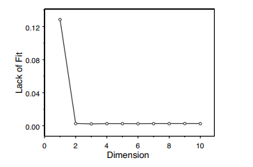
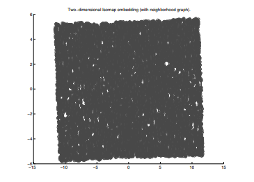
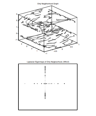
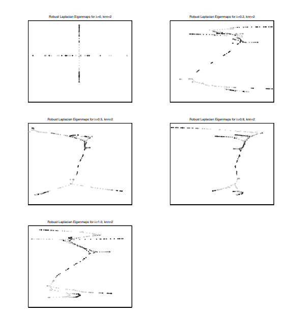
Figures $2.5-2.7$ show the results after using LEM for different values of $k$. As the value of $k$ increases from 1 to higher values we notice the spreading of the embedded data. The bottom subplot shows the nearest neighbor graph with $k=1$ as shown in Figure 2.7. The right plot shows the embedding of the graph. It is interesting to observe how the embedded data loses its local neighborhood information. The embedding practically happens along the second principal eigenvector (the first being Zero Vector). As the value of $k$ is increased to 2, we observe that embedding happens along the second and third principal axes. See Figure 2.7. For $k=1$ the graph is highly disconnected and for $k=2$ the graphs has much less isolated pieces of graphs. One interesting thing to observe is that as the connectivity of the graph increases the low-dimensional representation begins to preserve the local information.
The graph with $k=2$ and its embedding is shown in Figure 2.8. Increasing the neighborhood information to 2 neighbors is still not able to represent the continuity of the original manifold. Figure $2.7$ shows the graph with $k=3$ and its embedding. Increasing the neighborhood information to 3 neighbors better represents the continuity of the original manifold. Figure $2.5$ shows the graph with $k=5$ and its embedding. Increasing the neighborhood information to 5 neighbors better represents the continuity of the original manifold. Similar results are obtained by increasing the the number of neighbors, however, it should be noted that when the number of neighbors is very high then the graph starts to get influenced by ambient neigbhors.

We see similar results for the face images. The three plots in Figure $2.6$ show the embedding results obtained using LEM when the neighborhood graphs are created using $k=1, k=2$, and $k=5$. The top and the middle plot validate the limitation of LEM.

机器学习代写|流形学习代写manifold data learning代考|Bibliographical and Historical Remarks

Dimensionality reduction is an important research area in data analysis with an extensive research literature. Both linear and non-linear methods exist, and each category has both supervised and unsupervised versions. In this section we will briefly mention some of the salient works that have been proposed in the area of locally preserving manifold learning: see $[8]$ for a broader survey.

Lee and Seung [12] showed that many high dimensional data such as a series of related images, video frames, etc. lie on a much lower-dimensional manifold instead of being scattered throughout the feature space. This particular observation has motivated researchers to develop dimension reduction algorithms that try to learn an embedded manifold in a high-dimensional space.

ISOMAP [14] learns the manifold by exploring geodesic distances. In fact the algorithm tries to preserve the geometry of the data on the manifold by noting the points in the neighborhood of each point. The algorithm is defined as such:

Form a neighborhood graph $G$ for the dataset, based, for instance, on the $K$ nearest neighbors of each point $x_{i}$ –
For every pair of nodes in the graph, compute the shortest path, using Dijkstras algorithm, as an estimate of intrinsic distance on the data manifold. The weights of edges of the graphs are computed based on the Euclidean distance measure.
Classical Multi-Dimensional Scaling algorithm is computed using these pairwise distances to find a lower dimensional embedding $y_{i}$.

Bernstein et al. [22] have described the convergence properties of the estimation procedure for the intrinsic distances. For large and dense data sets, computation of pairwise distances is time consuming, and moreover the calculation of eigenvalues can be computationally intensive for large data sets. Such constraints have motivated researchers to find simpler variations of the Isomap algorithm. One such algorithm uses subsampled data called landmarks. Firstly, it calculates Isomap for random points called landmarks and between those landmarks a simple triangulation algorithm is applied.

Locally Linear Embedding (LLE) is an unsupervised learning method based on global and local optimization [11]. It is is similar to Isomap in the sense that it generates a graphical representation of the data set. However, it is different from Isomap as it only attempts to preserve local structures of the data. Because of the locality property used in LLE, the algorithm allows for successful embedding of nonconvex manifolds. An important point to be noted is that LLE creates the local properties of a manifold using the linear combinations of $k$ nearest neighbors of the data $x_{i}$. LLE attempts to create a local regression like model and thereby tries to fit a hyperplane through the data point $x_{i}$. This appears to be reasonable for smooth manifolds where the nearest neighbors align themselves well in a linear space. For very non-smooth or noisy data sets, LLE does not perform well. It has been noted that LLE preserves the reconstruction weights in the space of lower dimensionality, as the reconstruction weights of a data point are invariant to linear transformational operations like translation, rotation, etc.

机器学习代写|流形学习代写manifold data learning代考|Arkadas Ozakin, Nikolaos Vasiloglou II, Alexander Gray

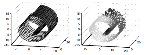
Much of the recent work in manifold learning and nonlinear dimensionality reduction focuses on distance-based methods, i.e., methods that aim to preserve the local or global (geodesic) distances between data points on a submanifold of Euclidean space. While this is a promising approach when the data manifold is known to have no intrinsic curvature (which is the case for common examples such as the “Swiss roll”), classical results in Riemannian geometry show that it is impossible to map a $d$-dimensional data manifold with intrinsic curvature into $\mathbb{R}^{d}$ in a manner that preserves distances. Consequently, distance-based methods of dimensionality reduction distort intrinsically curved data spaces, and they often do so in unpredictable ways. In this chapter, we discuss an alternative paradigm of manifold learning. We show that it is possible to perform nonlinear dimensionality reduction by preserving the underlying density of the data, for a much larger class of data manifolds than intrinsically flat ones, and demonstrate a proof-of-concept algorithm demonstrating the promise of this approach.

Visual inspection of data after dimensional reduction to two or three dimensions is among the most common uses of manifold learning and nonlinear dimensionality reduction. Typically, what is sought by the user’s eye in two or three-dimensional plots is clustering and other relationships in the data. Knowledge of the density, in principle, allows one to identify such basic structures as clusters and outliers, and even define nonparametric classifiers; the underlying density of a data set is arguably one of the most fundamental statistical objects that describe it. Thus, a method of dimensionality reduction that is guaranteed to preserve densities may well be preferable to methods that aim to preserve distances, but end up distorting them in uncontrolled ways.

Many of the manifold learning methods require the user to set a neighborhood radius $h$, or, for $k$-nearest neighbor approaches, a positive integer $k$, to be used in determining the neighborhood graph. Most of the time, there is no automatic way to pick the appropriate values of the tweak parameters $h$ and $k$, and one resorts to trial and error, looking for values that result in reasonable-looking plots. Kernel density estimation, one of the most popular and useful methods of estimating the underlying density of a data set, comes with a natural way to choose $h$ or $k$; it suggests to us to pick the value that maximizes a cross-validation score for the density estimate. While the usual kernel density estimation does not allow one to estimate the density of data on submanifolds of Euclidean space, a small modification

allows one to do so. This modification and its ramifications are discussed below in the context of density-preserving maps.

The chapter is organized as follows. In Section 3.2, using a theorem of Moser, we prove the existence of density preserving maps into $\mathbb{R}^{d}$ for a large class of $d$-dimensional manifolds, and give an intuitive discussion on the nonuniqueness of such maps. In Section 3.3, we describe a method for estimating the underlying density of a data set on a Riemannian submanifold of Euclidean space. We state the main result on the consistency of this submanifold density estimator, and give a bound on its convergence rate, showing that the latter is determined by the intrinsic dimensionality of the data instead of the full dimensionality of the feature space. This, incidentally, shows that the curse of dimensionality in the widely-used method of kernel density estimation is not as severe as is generally believed, if the method is properly modified for data on submanifolds. In Section 3.4, using a modified version of the estimator defined in Section 3.3, we describe a proof-of-concept algorithm for density preserving maps based on semidefinite programming, and give experimental results. Finally, in Sections $7.7$ and 3.6, we summarize the chapter and discuss relevant bibliography.

机器学习代写|流形学习代写manifold data learning代考|LEM Results

数据2.5−2.7显示使用 LEM 处理不同值后的结果ķ. 作为价值ķ从 1 增加到更高的值，我们注意到嵌入数据的传播。底部子图显示最近邻图ķ=1如图 2.7 所示。右图显示了图形的嵌入。观察嵌入数据如何丢失其本地邻域信息是很有趣的。嵌入实际上沿着第二个主特征向量（第一个是零向量）发生。作为价值ķ增加到 2，我们观察到嵌入发生在第二和第三主轴上。请参见图 2.7。为了ķ=1该图高度不连贯，并且对于ķ=2这些图的孤立图块要少得多。要观察的一件有趣的事情是，随着图的连通性增加，低维表示开始保留局部信息。
该图与ķ=2其嵌入如图 2.8 所示。将邻域信息增加到 2 个邻居仍然无法表示原始流形的连续性。数字2.7显示图表ķ=3及其嵌入。将邻域信息增加到 3 个邻居更好地代表了原始流形的连续性。数字2.5显示图表ķ=5及其嵌入。将邻域信息增加到 5 个邻居更好地代表了原始流形的连续性。通过增加邻居的数量可以获得类似的结果，但是应该注意的是，当邻居的数量非常高时，图开始受到环境邻居的影响。

我们看到面部图像的类似结果。图中的三个地块2.6显示使用 LEM 创建邻域图时使用 LEM 获得的嵌入结果ķ=1,ķ=2，和ķ=5. 上图和中图验证了 LEM 的局限性。

机器学习代写|流形学习代写manifold data learning代考|Bibliographical and Historical Remarks

降维是数据分析中的一个重要研究领域，具有广泛的研究文献。线性和非线性方法都存在，每个类别都有监督和无监督版本。在本节中，我们将简要提及在局部保留流形学习领域提出的一些突出工作：参见[8]进行更广泛的调查。

Lee 和 Seung [12] 表明，许多高维数据（例如一系列相关图像、视频帧等）位于低得多的流形上，而不是分散在整个特征空间中。这一特殊观察促使研究人员开发降维算法，试图在高维空间中学习嵌入式流形。

ISOMAP [14] 通过探索测地距离来学习流形。事实上，该算法试图通过注意每个点附近的点来保留流形上数据的几何形状。算法定义如下：

形成邻域图G对于数据集，例如，基于ķ每个点的最近邻X一世 –
对于图中的每一对节点，使用 Dijkstras 算法计算最短路径，作为数据流形上内在距离的估计。图的边权重是根据欧几里得距离度量计算的。
使用这些成对距离计算经典的多维缩放算法以找到较低维的嵌入是一世.

伯恩斯坦等人。[22]已经描述了内在距离估计过程的收敛特性。对于大而密集的数据集，成对距离的计算非常耗时，而且对于大数据集，特征值的计算可能是计算密集型的。这种约束促使研究人员寻找 Isomap 算法的更简单的变体。一种这样的算法使用称为地标的二次采样数据。首先，它为称为界标的随机点计算 Isomap，并在这些界标之间应用简单的三角测量算法。

局部线性嵌入 (LLE) 是一种基于全局和局部优化的无监督学习方法 [11]。在生成数据集的图形表示方面，它类似于 Isomap。但是，它与 Isomap 不同，因为它仅尝试保留数据的局部结构。由于 LLE 中使用的局部性属性，该算法允许成功嵌入非凸流形。需要注意的重要一点是，LLE 使用以下的线性组合创建流形的局部属性ķ数据的最近邻X一世. LLE 尝试创建类似于模型的局部回归，从而尝试通过数据点拟合超平面X一世. 这对于最近的邻居在线性空间中很好地对齐的平滑流形来说似乎是合理的。对于非常不平滑或嘈杂的数据集，LLE 表现不佳。已经注意到，LLE 保留了低维空间中的重建权重，因为数据点的重建权重对于平移、旋转等线性变换操作是不变的。

机器学习代写|流形学习代写manifold data learning代考|Arkadas Ozakin, Nikolaos Vasiloglou II, Alexander Gray

最近在流形学习和非线性降维方面的大部分工作都集中在基于距离的方法上，即旨在保持欧几里得空间子流形上数据点之间的局部或全局（测地线）距离的方法。当已知数据流形没有内在曲率时，这是一种很有前途的方法（常见的例子就是“瑞士卷”），黎曼几何中的经典结果表明，不可能映射一个d具有内在曲率的维数据流形Rd以保持距离的方式。因此，基于距离的降维方法扭曲了本质上弯曲的数据空间，并且它们通常以不可预测的方式这样做。在本章中，我们将讨论流形学习的另一种范式。我们展示了通过保留数据的基础密度来执行非线性降维是可能的，对于比本质上平坦的数据流形更大的数据流形类别，并演示了一种概念验证算法，证明了这种方法的前景。

降维到二维或三维后的数据视觉检查是流形学习和非线性降维的最常见用途之一。通常，用户在二维或三维图中寻找的是数据中的聚类和其他关系。原则上，对密度的了解可以让人们识别诸如簇和异常值之类的基本结构，甚至可以定义非参数分类器；数据集的潜在密度可以说是描述它的最基本的统计对象之一。因此，保证保持密度的降维方法可能比旨在保持距离但最终以不受控制的方式扭曲它们的方法更可取。

许多流形学习方法需要用户设置邻域半径H, 或者, 对于ķ-最近邻方法，一个正整数ķ，用于确定邻域图。大多数时候，没有自动方法来选择调整参数的适当值H和ķ，并且一个人诉诸试验和错误，寻找导致看起来合理的图的值。核密度估计是估计数据集底层密度的最流行和最有用的方法之一，它提供了一种自然的选择方式H或者ķ; 它建议我们选择最大化密度估计的交叉验证分数的值。虽然通常的核密度估计不允许人们估计欧几里得空间子流形上的数据密度，但一个小的修改

允许这样做。这种修改及其后果将在下面的密度保持地图的背景下讨论。

本章组织如下。在第 3.2 节中，使用 Moser 定理，我们证明了密度保持映射的存在Rd对于一大类d维流形，并直观地讨论此类映射的非唯一性。在 3.3 节中，我们描述了一种估计欧几里得空间的黎曼子流形上数据集的潜在密度的方法。我们陈述了这个子流形密度估计器一致性的主要结果，并给出了它的收敛速度的界限，表明后者是由数据的固有维度而不是特征空间的全维度决定的。顺便说一句，这表明，如果对子流形数据进行适当修改，则广泛使用的核密度估计方法中的维数灾难并不像通常认为的那么严重。在第 3.4 节中，使用第 3.3 节中定义的估计器的修改版本，我们描述了一种基于半定规划的密度保持图的概念验证算法，并给出了实验结果。最后，在部分7.73.6，我们总结本章并讨论相关参考书目。

机器学习代写|流形学习代写manifold data learning代考请认准statistics-lab™

统计代写请认准statistics-lab™. statistics-lab™为您的留学生涯保驾护航。

金融工程代写

金融工程是使用数学技术来解决金融问题。金融工程使用计算机科学、统计学、经济学和应用数学领域的工具和知识来解决当前的金融问题，以及设计新的和创新的金融产品。

非参数统计代写

非参数统计指的是一种统计方法，其中不假设数据来自于由少数参数决定的规定模型；这种模型的例子包括正态分布模型和线性回归模型。

广义线性模型代考

广义线性模型（GLM）归属统计学领域，是一种应用灵活的线性回归模型。该模型允许因变量的偏差分布有除了正态分布之外的其它分布。

术语广义线性模型（GLM）通常是指给定连续和/或分类预测因素的连续响应变量的常规线性回归模型。它包括多元线性回归，以及方差分析和方差分析（仅含固定效应）。

有限元方法代写

有限元方法（FEM）是一种流行的方法，用于数值解决工程和数学建模中出现的微分方程。典型的问题领域包括结构分析、传热、流体流动、质量运输和电磁势等传统领域。

有限元是一种通用的数值方法，用于解决两个或三个空间变量的偏微分方程（即一些边界值问题）。为了解决一个问题，有限元将一个大系统细分为更小、更简单的部分，称为有限元。这是通过在空间维度上的特定空间离散化来实现的，它是通过构建对象的网格来实现的：用于求解的数值域，它有有限数量的点。边界值问题的有限元方法表述最终导致一个代数方程组。该方法在域上对未知函数进行逼近。[1] 然后将模拟这些有限元的简单方程组合成一个更大的方程系统，以模拟整个问题。然后，有限元通过变化微积分使相关的误差函数最小化来逼近一个解决方案。

tatistics-lab作为专业的留学生服务机构，多年来已为美国、英国、加拿大、澳洲等留学热门地的学生提供专业的学术服务，包括但不限于Essay代写，Assignment代写，Dissertation代写，Report代写，小组作业代写，Proposal代写，Paper代写，Presentation代写，计算机作业代写，论文修改和润色，网课代做，exam代考等等。写作范围涵盖高中，本科，研究生等海外留学全阶段，辐射金融，经济学，会计学，审计学，管理学等全球99%专业科目。写作团队既有专业英语母语作者，也有海外名校硕博留学生，每位写作老师都拥有过硬的语言能力，专业的学科背景和学术写作经验。我们承诺100%原创，100%专业，100%准时，100%满意。

随机分析代写

随机微积分是数学的一个分支，对随机过程进行操作。它允许为随机过程的积分定义一个关于随机过程的一致的积分理论。这个领域是由日本数学家伊藤清在第二次世界大战期间创建并开始的。

时间序列分析代写

随机过程，是依赖于参数的一组随机变量的全体，参数通常是时间。随机变量是随机现象的数量表现，其时间序列是一组按照时间发生先后顺序进行排列的数据点序列。通常一组时间序列的时间间隔为一恒定值（如1秒，5分钟，12小时，7天，1年），因此时间序列可以作为离散时间数据进行分析处理。研究时间序列数据的意义在于现实中，往往需要研究某个事物其随时间发展变化的规律。这就需要通过研究该事物过去发展的历史记录，以得到其自身发展的规律。

回归分析代写

多元回归分析渐进（Multiple Regression Analysis Asymptotics）属于计量经济学领域，主要是一种数学上的统计分析方法，可以分析复杂情况下各影响因素的数学关系，在自然科学、社会和经济学等多个领域内应用广泛。

MATLAB代写

MATLAB 是一种用于技术计算的高性能语言。它将计算、可视化和编程集成在一个易于使用的环境中，其中问题和解决方案以熟悉的数学符号表示。典型用途包括：数学和计算算法开发建模、仿真和原型制作数据分析、探索和可视化科学和工程图形应用程序开发，包括图形用户界面构建MATLAB 是一个交互式系统，其基本数据元素是一个不需要维度的数组。这使您可以解决许多技术计算问题，尤其是那些具有矩阵和向量公式的问题，而只需用 C 或 Fortran 等标量非交互式语言编写程序所需的时间的一小部分。MATLAB 名称代表矩阵实验室。MATLAB 最初的编写目的是提供对由 LINPACK 和 EISPACK 项目开发的矩阵软件的轻松访问，这两个项目共同代表了矩阵计算软件的最新技术。MATLAB 经过多年的发展，得到了许多用户的投入。在大学环境中，它是数学、工程和科学入门和高级课程的标准教学工具。在工业领域，MATLAB 是高效研究、开发和分析的首选工具。MATLAB 具有一系列称为工具箱的特定于应用程序的解决方案。对于大多数 MATLAB 用户来说非常重要，工具箱允许您学习和应用专业技术。工具箱是 MATLAB 函数（M 文件）的综合集合，可扩展 MATLAB 环境以解决特定类别的问题。可用工具箱的领域包括信号处理、控制系统、神经网络、模糊逻辑、小波、仿真等。

R语言代写	问卷设计与分析代写
PYTHON代写	回归分析与线性模型代写
MATLAB代写	方差分析与试验设计代写
STATA代写	机器学习/统计学习代写
SPSS代写	计量经济学代写
EVIEWS代写	时间序列分析代写
EXCEL代写	深度学习代写
SQL代写	各种数据建模与可视化代写

机器学习代写|流形学习代写manifold data learning代考|Robust Laplacian Eigenmaps Using Global Information

Posted on 2022年5月10日2022年5月10日 by statistics-lab

如果你也在怎样代写流形学习manifold data learning这个学科遇到相关的难题，请随时右上角联系我们的24/7代写客服。

我们提供的流形学习manifold data learning及其相关学科的代写，服务范围广, 其中包括但不限于:

Statistical Inference 统计推断
Statistical Computing 统计计算
Advanced Probability Theory 高等概率论
Advanced Mathematical Statistics 高等数理统计学
(Generalized) Linear Models 广义线性模型
Statistical Machine Learning 统计机器学习
Longitudinal Data Analysis 纵向数据分析
Foundations of Data Science 数据科学基础

机器学习代写|流形学习代写manifold data learning代考|Robust Laplacian Eigenmaps Using Global Information

机器学习代写|流形学习代写manifold data learning代考|Shounak Roychowdhury and Joydeep Ghosh

Dimensionality reduction is an important process that is often required to understand the data in a more tractable and humanly comprehensible way. This process has been extensively studied in terms of linear methods such as Principal Component Analysis (PCA), Independent Component Analysis (ICA), Factor Analysis etc. [8]. However, it has been noticed that many high dimensional data, such as a series of related images, lie on a manifold $[12]$ and are not scattered throughout the feature space.

Belkin and Niyogi in [2] proposed Laplacian Eigenmaps (LEM), a method that approximates the Laplace-Beltrami Operator which is able to capture the properties of any Riemaniann manifold. The motivation of our work derives from our experimental observations that when the graph that used Laplacian Eigenmaps (LEM) [2] is not well-constructed (either it has lot of isolated vertices or there are islands of subgraphs) the data is difficult to interpret after a dimension reduction. This paper discusses how global information can be used in addition to local information in the framework of Laplacian Eigenmaps to address such situations. We make use of an interesting result by Costa and Hero that shows that Minimum Spanning Tree on a manifold can reveal its intrinsic dimension and entropy [4]. In other words, it implies that MSTs can capture the underlying global structure of the manifold if it exists. We use this finding to extend the dimension reduction technique using LEM to exploit both local and global information.

LEM depends on the Graph Laplacian matrix and so does our work. Fiedler initially proposed the Graph Laplacian matrix as a means to comprehend the notion of algebraic connectivity of a graph [6]. Merris has extensively discussed the wide variety of properties of the Laplacian matrix of a graph such as invariance, on various bounds and inequalities, extremal examples and constructions, etc., in his survey [10]. A broader role of the Laplacian matrix can be seen in Chung’s book on Spectral Graph Theory [3].

The second section touches on the Graph Laplacian matrix. The role of global information in manifold learning is then presented, followed by our proposed approach of augmenting LEM by including global information about the data. Experimental results confirm that global information can indeed help when the local information is limited for manifold learning.

机器学习代写|流形学习代写manifold data learning代考|Graph Laplacian

Let us consider a weighted graph $G=(V, E)$, where $V=V(G)=\left{v_{1}, v_{2}, \ldots, v_{n}\right}$ is the set of vertices (also called vertex set) and $E=E(G)=\left{e_{1}, e_{2}, \ldots, e_{n}\right}$ is the set of edges (also called edge set). The weight $w$ function is defined as $w: V \times V \rightarrow \Re$ such that $w\left(v_{i}, v_{j}\right)=w\left(v_{j}, v_{i}\right)=w_{i j}$.
Definition 1: The Laplacian [6] of a graph without loops of multiple edges is defined as the following:
$$
L(G)= \begin{cases}d_{v_{i}} & \text { if } v_{i}=v_{j} \ -1 & \text { if } v_{i} \text { are } v_{j} \text { adjacent } \ 0 & \text { Otherwise }\end{cases}
$$
Fiedler [6] defined the Laplacian of a graph as a symmetric matrix for a regular graph, where $A$ is an adjacency matrix ( $A^{T}$ is the transpose of adjacency matrix), $I$ is the identity matrix, and $n$ is the degree of the regular graph:
$$
L(G)=n I-A .
$$
A definition by Chung (see [3]) – which is given below – generalizes the Laplacian by adding the weights on the edges of the graph. It can be viewed as Weighed Graph Laplacian. Simply, it is a difference between the diagonal matrix $D$ and $W$, the weighted adjacency matrix.
$$
L_{W}(G)=D-W,
$$
where the diagonal element in $D$ is defined as $d_{v_{i}}=\sum_{j=1}^{n} w\left(v_{i}, v_{j}\right)$.
Definition 2: The Laplacian of weighted graph (operator) is defined as the following:
$$
L_{w}(G)= \begin{cases}d_{v_{i}}-w\left(v_{i}, v_{j}\right) & \text { if } v_{i}=v_{j} \ -w\left(v_{i}, v_{j}\right) & \text { if } v_{i} \text { are } v_{j} \text { connected } \ 0 & \text { otherwise. }\end{cases}
$$
$L_{w}(G)$ reduces to $L(G)$ when the edges have unit weights.

机器学习代写|流形学习代写manifold data learning代考|Global Information of Manifold

Global information has not been used in manifold learning since it is widely believed that global information may capture unnecessary data (like ambient data points) that should be avoided when dealing with manifolds.

However, some recent research results show that that it might be useful to to explore global information in a more constrained manner for manifold learning. Costa and Hero show that it is possible to use a Geodesic Minimum Spanning Tree (GMST) on the manifold to estimate the intrinsic dimension and intrinsic entropy of the manifold [4].

Costa and Hero showed in the following theorem that is possible to learn the intrinsic entropy and intrinsic dimension of a non-linear manifold by extending the BHH theorem [1], a well-known result in Geometric Probability.

Theorem: [Generalization of BHH Theorem to Embedded manifolds: [4]] Let $\mathcal{M}$ be a smooth compact $m$-dimensional manifold embedded in $\mathbb{R}^{d}$ through the diffeomorphism $\phi: \Omega \rightarrow \mathcal{M}$, and $\Omega \in \mathbb{R}^{d}$. Assume $2 \leq m \leq d$ and $0<\gamma<m$. Suppose that $Y_{1}, Y_{2}, \ldots$ are iid random vectors on $\mathcal{M}$ having a common density function $f$ with respect to a Lebesgue measure $\mu_{\mathcal{M}}$ on $\mathcal{M}$. Then the length functional $T_{\gamma}^{\mathbb{R}^{m}} \phi_{-1}\left(Y_{n}\right)$ of the MST spanning $\phi^{-1}\left(Y_{n}\right)$ satisfies the equation shown below in an almost sure sense:

$$
\lim {n \rightarrow \infty} \frac{T{\gamma}^{2^{m}} \phi_{-1}\left(Y_{n}\right)}{n \frac{(d-1)}{d}}=
$$
where $\alpha=(m-\gamma) / m$, and is always between $0<\alpha<1, J$ is the Jacobian, and $\beta_{m}$ is $a$ constant which depends on $m$.

Based on the above theorem we use MST on the entire data set as a source of global information. For more details see $[4]$, and more background information see [15] and [13].
The basic principle of GLEM is quite straightforward. The objective function that is to be minimized is given by the following (it is has the same flavor and notation used in [2]):
$$
\begin{aligned}
& \sum_{i, j}\left|\mathbf{y}^{(\mathbf{i})}-\mathbf{y}^{(\mathbf{j})}\right|_{2}^{2}\left(W_{i j}^{N N}+W_{i j}^{M S T}\right) \
=& \operatorname{tr}\left(\mathbf{Y}^{T} L\left(G_{N N}\right) \mathbf{Y}+\mathbf{Y}^{T} L\left(G_{M S T}\right) \mathbf{Y}\right) \
=& \operatorname{tr}\left(\mathbf{Y}^{T}\left(L\left(G_{N N}\right)+L\left(G_{M S T}\right)\right) \mathbf{Y}\right) \
=& \operatorname{tr}\left(\mathbf{Y}^{T} L(J) \mathbf{Y}\right) .
\end{aligned}
$$
where $\mathbf{y}^{(i)}=\left[y_{1}(i), \ldots, y_{m}(i)\right]^{T}$, and $m$ is the dimension of embedding. $W_{i j}^{N N}$ and $W_{i j}^{M S T}$ are weighted matrices of k-Nearest Neighbor graph and the MST graph respectively. In other words, we have
$$
\operatorname{argmin}{\mathbf{Y T} \mathbf{Y}=\mathbf{I}} \mathbf{Y}^{T} L \mathbf{Y} $$ such that $Y=\left[\mathbf{y}{\mathbf{1}}, \mathbf{y}{\mathbf{2}}, \ldots, \mathbf{y}{\mathbf{m}}\right]$ and $\mathbf{y}^{(\mathbf{i})}$ is the $m$-dimensional representation of $i^{\text {th }}$ vertex. The solutions to this optimization problem are the eigenvectors of the generalized eigenvalue problem
$$
L \mathbf{Y}=\Lambda D \mathbf{Y}
$$
The GLEM algorithm is described in Algorithm $1 .$

流形学习代写

机器学习代写|流形学习代写manifold data learning代考|Shounak Roychowdhury and Joydeep Ghosh

降维是一个重要的过程，通常需要以更易于处理和人类理解的方式理解数据。这个过程已经在线性方法方面得到了广泛的研究，如主成分分析（PCA）、独立成分分析（ICA）、因子分析等[8]。然而，已经注意到许多高维数据，例如一系列相关图像，位于流形上[12]并且不会分散在整个特征空间中。

Belkin 和 Niyogi 在 [2] 中提出了 Laplacian Eigenmaps (LEM)，这是一种近似 Laplace-Beltrami 算子的方法，能够捕获任何黎曼流形的属性。我们工作的动机源于我们的实验观察，即当使用拉普拉斯特征图 (LEM) [2] 的图构造不完善（它有很多孤立的顶点或存在子图岛）时，数据很难解释降维后。本文讨论了如何在拉普拉斯特征图框架中使用全局信息和局部信息来解决这种情况。我们利用了 Costa 和 Hero 的一个有趣结果，该结果表明流形上的最小生成树可以揭示其内在维度和熵 [4]。换句话说，这意味着 MST 可以捕获流形的潜在全局结构（如果存在）。我们利用这一发现来扩展使用 LEM 的降维技术，以利用本地和全局信息。

LEM 依赖于图拉普拉斯矩阵，我们的工作也是如此。Fiedler 最初提出图拉普拉斯矩阵作为理解图的代数连通性概念的一种手段 [6]。Merris 在他的调查 [10] 中广泛讨论了图的拉普拉斯矩阵的各种属性，例如不变性、各种边界和不等式、极值示例和构造等。拉普拉斯矩阵的更广泛作用可以在 Chung 的关于谱图理论的书中看到 [3]。

第二部分涉及图拉普拉斯矩阵。然后介绍了全局信息在流形学习中的作用，然后是我们提出的通过包含有关数据的全局信息来增强 LEM 的方法。实验结果证实，当局部信息受限于流形学习时，全局信息确实可以提供帮助。

机器学习代写|流形学习代写manifold data learning代考|Graph Laplacian

让我们考虑一个加权图G=(在,和)，在哪里V=V(G)=\left{v_{1}, v_{2}, \ldots, v_{n}\right}V=V(G)=\left{v_{1}, v_{2}, \ldots, v_{n}\right}是顶点集（也称为顶点集）和E=E(G)=\left{e_{1}, e_{2}, \ldots, e_{n}\right}E=E(G)=\left{e_{1}, e_{2}, \ldots, e_{n}\right}是边的集合（也称为边集）。重量在函数定义为在:在×在→ℜ这样在(在一世,在j)=在(在j,在一世)=在一世j.
定义 1：没有多重边环的图的拉普拉斯算子 [6] 定义如下：
大号(G)={d在一世如果在一世=在j −1 如果在一世是在j 邻近的 0 除此以外
Fiedler [6] 将图的拉普拉斯算子定义为正则图的对称矩阵，其中一种是一个邻接矩阵 (一种吨是邻接矩阵的转置），一世是单位矩阵，并且n是正则图的度数：
大号(G)=n一世−一种.
Chung 的定义（见 [3]）——下面给出——通过在图的边缘上添加权重来概括拉普拉斯算子。它可以看作是加权图拉普拉斯算子。简单来说，就是对角矩阵的区别D和在，加权邻接矩阵。
大号在(G)=D−在,
其中对角线元素在D定义为d在一世=∑j=1n在(在一世,在j).
定义2：加权图（算子）的拉普拉斯算子定义如下：
大号在(G)={d在一世−在(在一世,在j) 如果在一世=在j −在(在一世,在j) 如果在一世是在j 连接的 0 除此以外。
大号在(G)减少到大号(G)当边有单位权重时。

机器学习代写|流形学习代写manifold data learning代考|Global Information of Manifold

全局信息尚未用于流形学习，因为人们普遍认为全局信息可能会捕获在处理流形时应避免的不必要数据（如环境数据点）。

然而，最近的一些研究结果表明，以更受约束的方式探索全局信息对于流形学习可能是有用的。Costa 和 Hero 表明，可以在流形上使用测地线最小生成树 (GMST) 来估计流形的内在维度和内在熵 [4]。

Costa 和 Hero 在以下定理中表明，可以通过扩展 BHH 定理 [1] 来学习非线性流形的内在熵和内在维数，这是几何概率中的一个众所周知的结果。

定理：[BHH 定理到嵌入流形的推广：[4]] 让米是一个光滑的紧凑米维流形嵌入Rd通过微分同胚φ:Ω→米，和Ω∈Rd. 认为2≤米≤d和0<C<米. 假设是1,是2,…是 iid 随机向量米具有共同的密度函数F关于 Lebesgue 测度μ米在米. 那么长度泛函吨CR米φ−1(是n)MST 跨越的φ−1(是n)几乎可以肯定地满足下面显示的方程：林n→∞吨C2米φ−1(是n)n(d−1)d=
在哪里一种=(米−C)/米, 并且总是介于0<一种<1,Ĵ是雅可比行列式，并且b米是一种常数取决于米.

基于上述定理，我们在整个数据集上使用 MST 作为全局信息的来源。有关更多详细信息，请参阅[4]，更多背景信息参见 [15] 和 [13]。
GLEM 的基本原理非常简单。要最小化的目标函数由以下给出（它与 [2] 中使用的风格和符号相同）：
∑一世,j|是(一世)−是(j)|22(在一世jññ+在一世j米小号吨) =tr⁡(是吨大号(Gññ)是+是吨大号(G米小号吨)是) =tr⁡(是吨(大号(Gññ)+大号(G米小号吨))是) =tr⁡(是吨大号(Ĵ)是).
在哪里是(一世)=[是1(一世),…,是米(一世)]吨，和米是嵌入的维度。在一世jññ和在一世j米小号吨分别是k-Nearest Neighbor图和MST图的加权矩阵。换句话说，我们有
精氨酸⁡是吨是=一世是吨大号是这样是=[是1,是2,…,是米]和是(一世)是个米-维表示一世th 顶点。这个优化问题的解是广义特征值问题的特征向量
大号是=ΛD是
GLEM 算法在算法中描述1.

统计代写请认准statistics-lab™. statistics-lab™为您的留学生涯保驾护航。

金融工程代写

非参数统计代写

非参数统计指的是一种统计方法，其中不假设数据来自于由少数参数决定的规定模型；这种模型的例子包括正态分布模型和线性回归模型。

广义线性模型代考

广义线性模型（GLM）归属统计学领域，是一种应用灵活的线性回归模型。该模型允许因变量的偏差分布有除了正态分布之外的其它分布。

有限元方法代写

随机分析代写

时间序列分析代写

回归分析代写

MATLAB代写

R语言代写	问卷设计与分析代写
PYTHON代写	回归分析与线性模型代写
MATLAB代写	方差分析与试验设计代写
STATA代写	机器学习/统计学习代写
SPSS代写	计量经济学代写
EVIEWS代写	时间序列分析代写
EXCEL代写	深度学习代写
SQL代写	各种数据建模与可视化代写

机器学习代写|流形学习代写manifold data learning代考|Diffusion Maps

Posted on 2022年5月10日2022年5月10日 by statistics-lab

如果你也在怎样代写流形学习manifold data learning这个学科遇到相关的难题，请随时右上角联系我们的24/7代写客服。

我们提供的流形学习manifold data learning及其相关学科的代写，服务范围广, 其中包括但不限于:

Statistical Inference 统计推断
Statistical Computing 统计计算
Advanced Probability Theory 高等概率论
Advanced Mathematical Statistics 高等数理统计学
(Generalized) Linear Models 广义线性模型
Statistical Machine Learning 统计机器学习
Longitudinal Data Analysis 纵向数据分析
Foundations of Data Science 数据科学基础

机器学习代写|流形学习代写manifold data learning代考|Diffusion Maps

The basic idea of Diffusion MaPs (Nadler, Lafon, Coifman, and Kevrekidis, 2005; Coifman and Lafon, 2006) uses a Markov chain constructed over a graph of the data points, followed by an eigenanalysis of the probability transition matrix of the Markov chain. As with the other algorithms in this Section, there are three steps in this algorithm, with the first and second steps the same as for Laplacian eigenmaps. Although a nearest-neighbor search (Step 1) was not explicitly considered in the above papers on diffusion maps as a means of constructing the graph (Step 2), a nearest-neighbor search is included in software packages for computing diffusion maps. For an example in astronomy of a diffusion map incorporating a nearest-neighbor search, see Freeman, Newman, Lee, Richards, and Schafer (2009).

Nearest-Neighbor Search. Fix an integer $K$ or an $\epsilon>0$. Define a $K$-neighborhood $N_{i}^{K}$ or an $\epsilon$-neighborhood $N_{i}^{e}$ of the point $\mathbf{x}{i}$ as in Step 1 of Laplacian eigenmaps. In general, let $N{i}$ denote the neighborhood of $\mathbf{x}_{i}$.Pairwise Adjacency Matrix. The $n$ data points $\left{\mathbf{x}{i}\right}$ in $\Re^{r}$ can be regarded as a graph $\mathcal{G}=\mathcal{G}(\mathcal{V}, \mathcal{E})$ with the data points playing the role of vertices $\mathcal{V}=\left{\mathbf{x}{1}, \ldots, \mathbf{x}{n}\right}$, and the set of edges $\mathcal{E}$ are the connection strengths (or weights), $w\left(\mathbf{x}{i}, \mathbf{x}{j}\right)$, between pairs of adjacent vertices, $$ w{i j}=w\left(\mathbf{x}{i}, \mathbf{x}{j}\right)= \begin{cases}\exp \left{-\frac{\left|\mathbf{x}{i}-\mathbf{x}{i}\right|^{2}}{2 \sigma^{2}}\right}, & \text { if } \mathbf{x}{j} \in N{i} \ 0, & \text { otherwise. }\end{cases}
$$
This is a Gaussian kernel with width $\sigma$; however, other kernels may be used. Kernels such as (1.52) ensure that the closer two points are to each other, the larger the value of $w$. For convenience in exposition, we will suppress the fact that the elements of most of the matrices depend upon the value of $\sigma$. Then, $\mathbf{W}=\left(w_{i j}\right)$ is a pairwise adjacency matrix between the $n$ points. To make the matrix $\mathbf{W}$ even more sparse, values of its entries that are smaller than some given threshold (i.e., the points in question are far apart from each other) can be set to zero. The graph $\mathcal{G}$ with weight matrix W gives information on the local geometry of the data.
Spectral embedding. Define $\mathbf{D}=\left(d_{i j}\right)$ to be a diagonal matrix formed from the matrix W by setting the diagonal elements, $d_{i i}=\sum_{j} w_{i j}$, to be the column sums of $\mathbf{W}$ and the off-diagonal elements to be zero. The $(n \times n)$ symmetric matrix $\mathbf{L}=\mathbf{D}-\mathbf{W}$ is the graph Laplacian for the graph $\mathcal{G}$. We are interested in the solutions of the generalized eigenequation, $\mathbf{L v}=\lambda \mathbf{D v}$, or, equivalently, of the matrix
$$
\mathbf{P}=\mathbf{D}^{-1 / 2} \mathbf{L} \mathbf{D}^{-1 / 2}=\mathbf{I}_{n}-\mathbf{D}^{-1 / 2} \mathbf{W} \mathbf{D}^{-1 / 2},
$$
which is the normalized graph Laplacian. The matrix $\mathbf{H}=e^{t \mathbf{P}}, t \geq 0$, is usually referred to as the heat kernel. By construction, $\mathbf{P}$ is a stochastic matrix with all row sums equal to one, and, thus, can be interpreted as defining a random walk on the graph $\mathcal{G}$.

机器学习代写|流形学习代写manifold data learning代考|Hessian Eigenmaps

Recall that, in certain situations, the convexity assumption for IsOMAP may be too restrictive. Instead, we may require that the manifold $\mathcal{M}$ be locally isometric to an open, connected subset of $\Re^{t}$. Popular examples include families of “articulated” images (i.e., translated or rotated images of the same object, possibly through time) that are found in a high-dimensional, digitized-image library (e.g., faces, pictures, handwritten numbers or letters). However, if the pixel elements of each 64 -pixel-by-64-pixel digitized image are represented as a 4,096 -dimensional vector in “pixel space,” it would be very difficult to show that the images really live on a low-dimensional manifold, especially if that image manifold is unknown.

We can model such images using a vector of smoothly varying articulation parameters $\boldsymbol{\theta} \in \boldsymbol{\Theta}$. For example, digitized images of a person’s face that are varied by pose and illumination can be parameterized by two pose parameters (expression [happy, sad, sleepy, surprised, wink] and glasses-no glasses) and a lighting direction (centerlight, leftlight, rightlight, normal); similarly, handwritten ” 2 “s appear to be parameterized essentially by two features, bottom loop and top arch (Tenenbaum, de Silva, and Langford, 2000; Roweis and Saul, 2000). To some extent, learning about an underlying image manifold depends upon whether the images are sufficiently scattered around the manifold and how good is the quality of digitization of each image?

HESSIAN EIGENMAPS (Donoho and Grimes, 2003b) were proposed for recovering manifolds of high-dimensional libraries of articulated images where the convexity assumption is often violated. Let $\Theta \subset \Re^{t}$ be the parameter space and suppose that $\phi: \Theta \rightarrow R^{r}$, where $t<r$. Assume $\mathcal{M}=\phi(\Theta)$ is a smooth manifold of articulated images. The isometry and convexity requirements of IsoMAP are replaced by the following weaker requirements:

Local Isometry: $\phi$ is a locally isometric embedding of $\Theta$ into $\Re^{r}$. For any point $\mathbf{x}^{\prime}$ in a sufficiently small neighborhood around each point $x$ on the manifold $\mathcal{M}$, the geodesic distance equals the Euclidean distance between their corresponding parameter points $\boldsymbol{\theta}, \boldsymbol{\theta}^{\prime} \in \Theta ;$ that is,
$$
d^{M}\left(\mathbf{x}, \mathbf{x}^{\prime}\right)=\left|\theta-\theta^{\prime}\right|_{\Theta+}
$$
where $\mathbf{x}=\phi(\boldsymbol{\theta})$ and $\mathbf{x}^{\prime}=\phi\left(\boldsymbol{\theta}^{\prime}\right)$
Connectedness: The parameter space $\theta$ is an open, connected subset of $\Omega^{t}$.
The goal is to recover the parameter vector $\boldsymbol{\theta}$ (up to a rigid motion).

机器学习代写|流形学习代写manifold data learning代考|Nonlinear PCA

Another way of dealing with nonlinear manifold learning is to construct nonlinear versions of linear manifold learning techniques. We have already seen how Isomap provides a nonlinear generalization of MDS. How can we generalize PCA to the nonlinear case? In this Section,

we briefly describe the basic ideas behind POLYNOMIAL PCA, PRINCIPAL CuRVES AND SURFACES, MULTILAYER AUTOASSOCIATIVE NEURAL NETWORKS, and KerneL PCA.
Polynomial PCA
There have been several different attempts to generalize PCA to data living on or near nonlinear manifolds of a lower-dimensional space than input space. The first such idea was to add to the set of $r$ input variables quadratic, cubic, or higher-degree polynomial transformations of those input variables, and then apply linear PCA. The result is POLYNOMIAL PCA (Gnanadesikan and Wilk, 1969), whose embedding coordinates are the eigenvectors corresponding to the smallest few eigenvalues of the expanded covariance matrix.

In the original study of polynomial PCA, the method was illustrated with a quadratic transformation of bivariate input variables. In this scenario, $\left(X_{1}, X_{2}\right)$ expands to become $\left(X_{1}, X_{2}, X_{1}^{2}, X_{2}^{2}, X_{1} X_{2}\right)$. This formulation is feasible, but for larger problems, the possibilities become more complicated. First, the variables in the expanded set will not be scaled in a uniform manner, so that standardization will be necessary, and second, the number of variables in the expanded set will increase rapidly with large $r$, which will lead to bigger computational problems. Gnanadesikan and Wilk’s article, however, gave rise to a variety of attempts to define a more general nonlinear version of PCA.
Principal Curves and Surfaces
The next attempt at creating a nonlinear PCA was PRINCIPAL CURVES AND SURFACES (Hastie, 1984; Hastie and Stuetzle, 1989). A principal curve is a smooth one-dimensional curve that passes through the “middle” of the data, and a principal surface (or principal manifold) is a generalization of a principal curve to a smooth two- or higher-dimensional manifold. So, we can visualize principal curves and surfaces as defining a nonlinear manifold in higher-dimensional input space.

Let $\mathbf{x} \in \Re^{r}$ be a data point and let $\mathbf{f}(\lambda)$ be a curve, $\lambda \in \Lambda$; see Section $1.2 .4$ for definitions. Project $\mathbf{x}$ to a point on $\mathbf{f}(\lambda)$ that is closest in Euclidean distance to $\mathbf{x}$. Define the projection index
$$
\lambda_{\mathbf{f}}(\mathbf{x})=\sup {\lambda}\left{\lambda:|\mathbf{x}-\mathbf{f}(\lambda)|=\inf {\mu}|\mathbf{x}-\mathbf{f}(\mu)|\right}
$$

流形学习代写

机器学习代写|流形学习代写manifold data learning代考|Diffusion Maps

Diffusion Maps 的基本思想（Nadler、Lafon、Coifman 和 Kevrekidis，2005 年；Coifman 和 Lafon，2006 年）使用在数据点图上构建的马尔可夫链，然后对马尔可夫链的概率转移矩阵进行特征分析. 与本节中的其他算法一样，该算法有三个步骤，第一步和第二步与拉普拉斯特征图相同。尽管在上述关于扩散图的论文中没有明确考虑最近邻搜索（步骤 1）作为构建图的一种手段（步骤 2），但最近邻搜索包含在用于计算扩散图的软件包中。有关包含最近邻搜索的扩散图的天文学示例，请参见 Freeman、Newman、Lee、Richards 和 Schafer (2009)。

最近邻搜索。修复一个整数ķ或一个ε>0. 定义一个ķ-邻里ñ一世ķ或一个ε-邻里ñ一世和点的X一世如拉普拉斯特征图的第 1 步。一般来说，让ñ一世表示邻域X一世.成对邻接矩阵。这n数据点\left{\mathbf{x}{i}\right}\left{\mathbf{x}{i}\right}在ℜr可以看成图G=G(在,和)数据点扮演顶点的角色\mathcal{V}=\left{\mathbf{x}{1}, \ldots, \mathbf{x}{n}\right}\mathcal{V}=\left{\mathbf{x}{1}, \ldots, \mathbf{x}{n}\right}, 和边的集合和是连接强度（或权重），在(X一世,Xj)，在相邻顶点对之间，$$ w{ij}=w\left(\mathbf{x}{i}, \mathbf{x}{j}\right)=\begin{cases}\exp \left{-\frac{\left|\mathbf{x}{i}-\mathbf{x}{i}\right|^{2}}{2 \sigma^{2} }\right}, & \text { if } \mathbf{x}{j} \in N{i} \ 0, & \text { 否则。}\结束{案例}\begin{cases}\exp \left{-\frac{\left|\mathbf{x}{i}-\mathbf{x}{i}\right|^{2}}{2 \sigma^{2} }\right}, & \text { if } \mathbf{x}{j} \in N{i} \ 0, & \text { 否则。}\结束{案例}
$$
这是一个具有宽度的高斯核σ; 但是，可以使用其他内核。（1.52）等内核保证两点距离越近，值越大在. 为方便说明，我们将隐藏大多数矩阵的元素取决于σ. 然后，在=(在一世j)是之间的成对邻接矩阵n点。制作矩阵在甚至更稀疏，其条目的值小于某个给定阈值（即，所讨论的点彼此相距很远）可以设置为零。图表G权重矩阵 W 给出了数据的局部几何信息。
光谱嵌入。定义D=(d一世j)是通过设置对角元素由矩阵 W 形成的对角矩阵，d一世一世=∑j在一世j, 为的列总和在和非对角线元素为零。这(n×n)对称矩阵大号=D−在是图的拉普拉斯算子G. 我们对广义特征方程的解感兴趣，大号在=λD在, 或者, 等价的, 矩阵
$$
\mathbf{P}=\mathbf{D}^{-1 / 2} \mathbf{L} \mathbf{D}^{-1 / 2}=\mathbf{I}_{n}-\mathbf{D }^{-1 / 2} \mathbf{W} \mathbf{D}^{-1 / 2},
$$
这是归一化图拉普拉斯算子。矩阵H=和吨磷,吨≥0, 通常称为热核。通过施工，磷是一个随机矩阵，所有行和都等于 1，因此可以解释为在图上定义随机游走G.

机器学习代写|流形学习代写manifold data learning代考|Hessian Eigenmaps

回想一下，在某些情况下，IsOMAP 的凸性假设可能过于严格。相反，我们可能要求流形米局部等距到一个开放的、连通的子集ℜ吨. 流行的例子包括在高维数字化图像库（例如，面孔、图片、手写数字或字母）中找到的“铰接”图像系列（即，同一对象的翻译或旋转图像，可能随着时间的推移） . 但是，如果每个 64 像素×64 像素的数字化图像的像素元素在“像素空间”中表示为 4,096 维向量，那么很难证明这些图像真的存在于低维空间中。流形，特别是如果该图像流形是未知的。

我们可以使用平滑变化的关节参数向量对此类图像进行建模θ∈θ. 例如，可以通过两个姿势参数（表情 [快乐、悲伤、困倦、惊讶、眨眼] 和不戴眼镜）和照明方向（中心光、左光, 右光, 正常); 类似地，手写的“2”似乎基本上由两个特征参数化，底部环和顶部拱（Tenenbaum、de Silva 和 Langford，2000；Roweis 和 Saul，2000）。在某种程度上，了解底层图像流形取决于图像是否充分分散在流形周围以及每个图像的数字化质量有多好？

HESSIAN EIGENMAPS (Donoho and Grimes, 2003b) 被提出用于恢复经常违反凸性假设的铰接图像的高维库的流形。让θ⊂ℜ吨是参数空间并假设φ:θ→Rr，在哪里吨<r. 认为米=φ(θ)是铰接图像的平滑流形。IsoMAP 的等距和凸度要求被以下较弱的要求取代：

局部等距：φ是一个局部等距嵌入θ进入ℜr. 对于任何一点X′在每个点周围足够小的邻域中X在歧管上米，测地线距离等于它们对应的参数点之间的欧几里得距离θ,θ′∈θ;那是，
d米(X,X′)=|θ−θ′|θ+
在哪里X=φ(θ)和X′=φ(θ′)
连通性：参数空间θ是一个开放的、连通的子集Ω吨.
目标是恢复参数向量θ（直到刚性运动）。

机器学习代写|流形学习代写manifold data learning代考|Nonlinear PCA

处理非线性流形学习的另一种方法是构建线性流形学习技术的非线性版本。我们已经看到 Isomap 如何提供 MDS 的非线性泛化。我们如何将 PCA 推广到非线性情况？在这个部分，

我们简要描述了多项式 PCA、主曲线和曲面、多层自关联神经网络和内核 PCA 背后的基本思想。
多项式 PCA
有几种不同的尝试将 PCA 推广到生活在比输入空间低维空间的非线性流形上或附近的数据。第一个这样的想法是添加到集合r输入变量对这些输入变量进行二次、三次或更高次多项式变换，然后应用线性 PCA。结果是 POLYNOMIAL PCA (Gnanadesikan and Wilk, 1969)，其嵌入坐标是对应于扩展协方差矩阵的最小几个特征值的特征向量。

在多项式 PCA 的原始研究中，该方法通过二元输入变量的二次变换来说明。在这种情况下，(X1,X2)展开成为(X1,X2,X12,X22,X1X2). 这个公式是可行的，但是对于更大的问题，可能性变得更加复杂。首先，扩展集中的变量不会以统一的方式缩放，因此需要标准化，其次，扩展集中的变量数量会随着较大的r，这将导致更大的计算问题。然而，Gnanadesikan 和 Wilk 的文章引发了各种尝试来定义更一般的非线性 PCA 版本。
主曲线和曲面
创建非线性 PCA 的下一个尝试是主曲线和曲面（Hastie，1984；Hastie 和 Stuetzle，1989）。主曲线是通过数据“中间”的平滑一维曲线，主曲面（或主流形）是主曲线向平滑二维或更高维流形的推广。因此，我们可以将主曲线和曲面可视化为在高维输入空间中定义非线性流形。

让X∈ℜr是一个数据点，让F(λ)成为曲线，λ∈Λ; 见部分1.2.4用于定义。项目X到一点F(λ)在欧几里得距离上最接近X. 定义投影索引
\lambda_{\mathbf{f}}(\mathbf{x})=\sup {\lambda}\left{\lambda:|\mathbf{x}-\mathbf{f}(\lambda)|=\inf { \mu}|\mathbf{x}-\mathbf{f}(\mu)|\right}

统计代写请认准statistics-lab™. statistics-lab™为您的留学生涯保驾护航。

金融工程代写

非参数统计代写

非参数统计指的是一种统计方法，其中不假设数据来自于由少数参数决定的规定模型；这种模型的例子包括正态分布模型和线性回归模型。

广义线性模型代考

广义线性模型（GLM）归属统计学领域，是一种应用灵活的线性回归模型。该模型允许因变量的偏差分布有除了正态分布之外的其它分布。

有限元方法代写

随机分析代写

时间序列分析代写

回归分析代写

MATLAB代写

R语言代写	问卷设计与分析代写
PYTHON代写	回归分析与线性模型代写
MATLAB代写	方差分析与试验设计代写
STATA代写	机器学习/统计学习代写
SPSS代写	计量经济学代写
EVIEWS代写	时间序列分析代写
EXCEL代写	深度学习代写
SQL代写	各种数据建模与可视化代写

机器学习代写|流形学习代写manifold data learning代考|Nonlinear Manifold Learning

Posted on 2022年5月10日2022年5月10日 by statistics-lab

如果你也在怎样代写流形学习manifold data learning这个学科遇到相关的难题，请随时右上角联系我们的24/7代写客服。

我们提供的流形学习manifold data learning及其相关学科的代写，服务范围广, 其中包括但不限于:

Statistical Inference 统计推断
Statistical Computing 统计计算
Advanced Probability Theory 高等概率论
Advanced Mathematical Statistics 高等数理统计学
(Generalized) Linear Models 广义线性模型
Statistical Machine Learning 统计机器学习
Longitudinal Data Analysis 纵向数据分析
Foundations of Data Science 数据科学基础

Principal Component Analysis explained visually — 机器学习代写|流形学习代写manifold data learning代考|Nonlinear Manifold Learning

机器学习代写|流形学习代写manifold data learning代考|Nonlinear Manifold Learning

We next discuss some algorithmic techniques that proved to be innovative in the study of nonlinear manifold learning: ISOMAP, LOCAL LINEAR EMBEDDING, LAPLACIAN EIGENMAPS, DIFFUSION MAPS, HESSIAN EIGENMAPS, and the many different versions of NONLINEAR PCA. The goal of each of these algorithms is to recover the full low-dimensional

representation of an unknown nonlinear manifold, $\mathcal{M}$, embedded in some high-dimensional space, where it is important to retain the neighborhood structure of $\mathcal{M}$. When $\mathcal{M}$ is highly nonlinear, such as the S-shaped manifold in the left panel of Figure $1.1$, these algorithms outperform the usual linear techniques. The nonlinear manifold-learning methods emphasize simplicity and avoid optimization problems that could produce local minima.

Assume that we have a finite random sample of data points, $\left{\mathbf{y}{i}\right}$, from a smooth $t$ dimensional manifold $\mathcal{M}$ with metric given by the geodesic distance $d^{\mathcal{M}} ;$ see Section $1.2 .4$. These points are then nonlinearly embedded by a smooth map $\psi$ into high-dimensional input space $\mathcal{X}=\Re^{r}(t \ll r)$ with Euclidean metric $|$. $| \mathcal{X}$. This embedding provides us with the input data $\left{\mathbf{x}{i}\right}$. For example, in the right panel of Figure $1.1$, we randomly generated 20,000 three-dimensional points to lie uniformly on the surface of the two-dimensional Sshaped curve displayed in the left panel. Thus, $\psi: \mathcal{M} \rightarrow \mathcal{X}$ is the embedding map, and a point on the manifold, $\mathbf{y} \in \mathcal{M}$, can be expressed as $\mathbf{y}=\phi(\mathbf{x}), \mathbf{x} \in \mathcal{X}$, where $\phi=\psi^{-1}$. The goal is to recover $\mathcal{M}$ and find an implicit representation of the map $\psi$ (and, hence, recover the $\left.\left{\mathbf{y}{i}\right}\right)$, given only the input data points $\left{\mathbf{x}{i}\right}$ in $\mathcal{X}$.

Each algorithm computes $t^{\prime}$-dimensional estimates, $\left{\widehat{\mathbf{y}}{i}\right}$, of the $t$-dimensional manifold data, $\left{\mathbf{y}{i}\right}$, for some $t^{\prime}$. Such a reconstruction is deemed to be successful if $t^{\prime}=t$, the true (unknown) dimensionality of $\mathcal{M}$. In practice, $t^{\prime}$ will most likely be too large. Because we require a low-dimensional solution, we retain only the first two or three of the coordinate vectors and plot the corresponding elements of those vectors against each other to yield $n$ points in two- or three-dimensional space. For all practical purposes, such a display is usually sufficient to identify the underlying manifold.

Most of the nonlinear manifold-learning algorithms that we discuss here are based upon different philosophies regarding how one should recover unknown nonlinear manifolds. However, they each consist of a three-step approach (except NONLINEAR PCA). The first and third steps are common to all algorithms: the first step incorporates neighborhood information at each data point to construct a weighted graph having the data points as vertices, and the third step is a spectral embedding step that involves an $(n \times n)$-eigenequation computation. The second step is specific to the algorithm, taking the weighted neighborhood graph and transforming it into suitable input for the spectral embedding step.

机器学习代写|流形学习代写manifold data learning代考|Isomap

The isometric feature mapping (or IsOMAP) algorithm (Tenenbaum, de Silva, and Langford, 2000 ) assumes that the smooth manifold $\mathcal{M}$ is a convex region of $\Re^{t}(t \ll r)$ and that the embedding $\psi: \mathcal{M} \rightarrow \mathcal{X}$ is an isometry. This assumption has two key ingredients:

Isometry: The geodesic distance is invariant under the map $\psi$. For any pair of points on the manifold, $\mathbf{y}, \mathbf{y}^{\prime} \in \mathcal{M}$, the geodesic distance between those points equals the Euclidean distance between their corresponding coordinates, $\mathbf{x}, \mathbf{x}^{\prime} \in \mathcal{X}$; i.e.,
$$
d^{\mathcal{M}}\left(\mathbf{y}, \mathbf{y}^{\prime}\right)=\left|\mathbf{x}-\mathbf{x}^{\prime}\right|_{\mathcal{X}}
$$
where $\mathbf{y}=\phi(\mathbf{x})$ and $\mathbf{y}^{\prime}=\phi\left(\mathbf{x}^{\prime}\right)$.
Convexity: The manifold $\mathcal{M}$ is a convex subset of $\Re^{t}$.
IsomaP considers $\mathcal{M}$ to be a convex region possibly distorted in any of a number of ways (e.g., by folding or twisting). The so-called Swiss roll, ${ }^{2}$ which is a flat two-dimensional rectangular submanifold of $\Re^{3}$, is one such example; see Figure $1.2$. Empirical studies show that IsOMAP works well for intrinsically flat submanifolds of $\mathcal{X}=\Re^{r}$ that look like rolledup sheets of paper or “open” manifolds such as an open box or open cylinder. However, IsOMAP does not perform well if there are any holes in the roll, because this would violate the convexity assumption. The isometry assumption appears to be reasonable for certain types of situations, but, in many other instances, the convexity assumption may be too restrictive (Donoho and Grimes, 2003b).

IsomAP uses the isometry and convexity assumptions to form a nonlinear generalization of multidimensional scaling (MDS). Recall that MDS looks for a low-dimensional subspace in which to embed input data while preserving the Euclidean interpoint distances (see Section 1.3.2). Unfortunately, working with Euclidean distances in MDS when dealing with curved regions tends to give poor results. IsOMAP follows the general MDS philosophy by attempting to preserve the global geometric properties of the underlying nonlinear manifold, and it does this by approximating all pairwise geodesic distances (i.e., lengths of the shortest paths between two points) on the manifold. In this sense, IsOMAP provides a global approach to manifold learning.

机器学习代写|流形学习代写manifold data learning代考|Laplacian Eigenmaps

The Laplacian eigenmap algorithm (Belkin and Niyogi, 2002) also consists of three steps. The first and third steps of the Laplacian eigenmap algorithm are very similar to the first and third steps, respectively, of the LLE algorithm.

Nearest-neighbor search. Fix an integer $K$ or an $\epsilon>0$. The neighborhoods of each data point are symmetrically defined: for a $K$-neighborhood $N_{i}^{K}$ of the point $\mathbf{x}{i}$, let $\mathbf{x}{j} \in N_{i}^{K}$ iff $\mathbf{x}{i} \in N{j}^{K}$; similarly, for an $\epsilon$-neighborhood $N_{i}^{\epsilon}$, let $\mathbf{x}{j} \in N{i}^{e}$ iff $\left|\mathbf{x}{i}-\mathbf{x}{j}\right|<\epsilon$, where the norm is Euclidean norm. In general, let $N_{i}$ denote the neighborhood of $\mathbf{x}_{i}$.
Weighted adjacency matrix. Let $\mathbf{W}=\left(w_{i j}\right)$ be a symmetric $(n \times n)$ weighted adjacency matrix defined as follows:
$$
w_{i j}=w\left(\mathbf{x}{i}, \mathbf{x}{j}\right)= \begin{cases}\exp \left{-\frac{\left|\mathbf{x}{i}-\mathbf{x}{j}\right|^{2}}{2 \sigma^{2}}\right}, & \text { if } \mathbf{x}{j} \in N{i} \ 0, & \text { otherwise }\end{cases}
$$

These weights are determined by the isotropic Gaussian kernel (also known as the heat kernel), with scale parameter $\sigma$. Denote the resulting weighted graph by $\mathcal{G}$. If $\mathcal{G}$ is not connected, apply step 3 to each connected subgraph.

Spectral embedding. Let $\mathbf{D}=\left(d_{i j}\right)$ be an $(n \times n)$ diagonal matrix with diagonal elements $d_{i i}=\sum_{j \in N_{i}} w_{i j}=\left(\mathbf{W} 1_{n}\right){i}, i=1,2, \ldots, n$. The $(n \times n)$ symmetric matrix $\mathbf{L}=\mathbf{D}-\mathbf{W}$ is known as the graph Laplacian for the graph $\mathcal{G}$. Let $\mathbf{y}=\left(y{i}\right)$ be an $n$-vector. Then, $\mathbf{y}^{\tau} \mathbf{L} \mathbf{y}=\frac{1}{2} \sum_{i=1}^{n} \sum_{j=1}^{n} w_{i j}\left(y_{i}-y_{j}\right)^{2}$, so that $\mathbf{L}$ is nonnegative definite.

When data are uniformly sampled from a low-dimensional manifold $\mathcal{M}$ of $\Re^{r}$, the graph Laplacian $\mathbf{L}=\mathbf{L}{n, \sigma}$ (considered as a function of $n$ and $\sigma$ ) can be regarded as a discrete approximation to the continuous Laplace-Beltrami operator $\Delta{\mathcal{M}}$ defined on the manifold $\mathcal{M}$, and converges to $\Delta_{\mathcal{M}}$ as $\sigma \rightarrow 0$ and $n \rightarrow \infty$. Furthermore, when the data are sampled from an arbitrary probability distribution $P$ on the manifold $\mathcal{M}$, then, under certain conditions on $\mathcal{M}$ and $P$, the graph Laplacian converges to a weighted version of $\Delta_{\mathcal{M}}$ (Belkin and Niyogi, 2008).

The $(t \times n)$-matrix $\mathbf{Y}=\left(\mathbf{y}{1}, \cdots, \mathbf{y}{n}\right)$, which is used to embed the graph $\mathcal{G}$ into the low-dimensional space $\Re^{t}$, where $\mathbf{y}{i}$ yields the embedding coordinates of the $i$ th point, is determined by minimizing the objective function, $$ \sum{i} \sum_{j} w_{i j}\left|\mathbf{y}{i}-\mathbf{y}{j}\right|^{2}=\operatorname{tr}\left{\mathbf{Y L Y} \mathbf{Y}^{\tau}\right}
$$
In other words, we seek the solution,
$$
\widehat{\mathbf{Y}}=\arg \min {\mathbf{Y}: \mathbf{Y D \mathbf { Y } ^ { \top } = \mathbf { I } { t }}} \operatorname{tr}\left{\mathbf{Y L Y ^ { \top } }},\right.
$$
where we restrict $\mathbf{Y}$ such that $\mathbf{Y D Y} \mathbf{Y}^{\tau}=\mathbf{I}{t}$ to prevent a collapse onto a subspace of fewer than $t-1$ dimensions. The solution is given by the generalized eigenequation, $\mathbf{L v}=\lambda \mathbf{D v}$, or, equivalently, by finding the eigenvalues and eigenvectors of the matrix $\widehat{\mathbf{W}}=\mathbf{D}^{-1 / 2} \mathbf{W D} \mathbf{D}^{-1 / 2}$. The smallest eigenvalue, $\lambda{n}$, of $\widehat{\mathbf{W}}$ is zero. If we ignore the smallest eigenvalue (and its corresponding constant eigenvector $\mathbf{v}{n}=1{n}$ ), then the best embedding solution in $\Re^{t}$ is similar to that given by LLE; that is, the rows of $\widehat{\mathbf{Y}}$ are the eigenvectors,
$$
\widehat{\mathbf{Y}}=\left(\widehat{\mathbf{y}}{1}, \cdots, \widehat{\mathbf{y}}{n}\right)=\left(\mathbf{v}{n-1}, \cdots, \mathbf{v}{n-t}\right)^{\tau},
$$
corresponding to the next $t$ smallest eigenvalues, $\lambda_{n-1} \leq \cdots \leq \lambda_{n-t}$, of $\widehat{\mathbf{W}}$.

流形学习代写

机器学习代写|流形学习代写manifold data learning代考|Nonlinear Manifold Learning

我们接下来讨论一些在非线性流形学习研究中被证明具有创新性的算法技术：ISOMAP、局部线性嵌入、拉普拉斯特征图、扩散图、黑森特征图以及许多不同版本的非线性 PCA。这些算法中的每一个的目标都是恢复完整的低维

未知非线性流形的表示，米，嵌入在一些高维空间中，其中保留邻域结构很重要米. 什么时候米是高度非线性的，例如图左面板中的 S 形流形1.1，这些算法优于通常的线性技术。非线性流形学习方法强调简单性并避免可能产生局部最小值的优化问题。

假设我们有一个有限的随机数据点样本，\left{\mathbf{y}{i}\right}\left{\mathbf{y}{i}\right}，从平滑吨多维流形米由测地距离给出的度量d米;见部分1.2.4. 然后这些点被平滑的地图非线性嵌入ψ进入高维输入空间X=ℜr(吨≪r)欧几里得度量|. |X. 这种嵌入为我们提供了输入数据\left{\mathbf{x}{i}\right}\left{\mathbf{x}{i}\right}. 例如，在图的右侧面板中1.1，我们随机生成了 20,000 个三维点，均匀地分布在左侧面板中显示的二维 S 形曲线的表面上。因此，ψ:米→X是嵌入图，是流形上的一个点，是∈米, 可以表示为是=φ(X),X∈X，在哪里φ=ψ−1. 目标是恢复米并找到地图的隐式表示ψ（因此，恢复\left.\left{\mathbf{y}{i}\right}\right)\left.\left{\mathbf{y}{i}\right}\right)，仅给定输入数据点\left{\mathbf{x}{i}\right}\left{\mathbf{x}{i}\right}在X.

每个算法计算吨′维估计，\left{\widehat{\mathbf{y}}{i}\right}\left{\widehat{\mathbf{y}}{i}\right}，的吨维流形数据，\left{\mathbf{y}{i}\right}\left{\mathbf{y}{i}\right}，对于一些吨′. 这种重建被认为是成功的，如果吨′=吨, 的真实（未知）维度米. 在实践中，吨′很可能会太大。因为我们需要一个低维解，我们只保留前两个或三个坐标向量，并将这些向量的对应元素相互绘制以产生n二维或三维空间中的点。出于所有实际目的，这种显示通常足以识别下面的歧管。

我们在这里讨论的大多数非线性流形学习算法都基于关于如何恢复未知非线性流形的不同哲学。但是，它们每个都包含一个三步方法（NONLINEAR PCA 除外）。第一步和第三步对所有算法都是通用的：第一步结合每个数据点的邻域信息，构建以数据点为顶点的加权图，第三步是谱嵌入步骤，涉及(n×n)-特征方程计算。第二步是特定于算法的，采用加权邻域图并将其转换为适合谱嵌入步骤的输入。

机器学习代写|流形学习代写manifold data learning代考|Isomap

等距特征映射（或 IsOMAP）算法（Tenenbaum、de Silva 和 Langford，2000 年）假设平滑流形米是一个凸区域ℜ吨(吨≪r)并且嵌入ψ:米→X是等距。这个假设有两个关键因素：

等距：测地线距离在地图下是不变的ψ. 对于流形上的任意一对点，是,是′∈米，这些点之间的测地线距离等于它们对应坐标之间的欧几里得距离，X,X′∈X; IE，
d米(是,是′)=|X−X′|X
在哪里是=φ(X)和是′=φ(X′).
凸性：流形米是一个凸子集ℜ吨.
IsomaP 认为米成为可能以多种方式（例如，通过折叠或扭曲）中的任何一种方式扭曲的凸面区域。所谓的瑞士卷，2它是一个平面二维矩形子流形ℜ3, 就是这样一个例子；见图1.2. 实证研究表明，IsOMAP 适用于本质平坦的子流形X=ℜr看起来像卷起的纸或“打开”的歧管，例如打开的盒子或打开的圆柱体。但是，如果卷中有任何孔洞，IsOMAP 的性能就不会很好，因为这会违反凸性假设。对于某些类型的情况，等距假设似乎是合理的，但在许多其他情况下，凸性假设可能过于严格（Donoho 和 Grimes，2003b）。

IsomAP 使用等距和凸性假设来形成多维尺度 (MDS) 的非线性泛化。回想一下，MDS 寻找一个低维子空间，在其中嵌入输入数据，同时保留欧几里德点间距离（参见第 1.3.2 节）。不幸的是，在处理弯曲区域时，在 MDS 中使用欧几里德距离往往会产生较差的结果。IsOMAP 遵循一般 MDS 哲学，试图保留底层非线性流形的全局几何特性，它通过近似流形上的所有成对测地线距离（即两点之间的最短路径的长度）来做到这一点。从这个意义上说，IsOMAP 为流形学习提供了一种全局方法。

机器学习代写|流形学习代写manifold data learning代考|Laplacian Eigenmaps

拉普拉斯特征图算法（Belkin 和 Niyogi，2002）也包括三个步骤。Laplacian eigenmap 算法的第一步和第三步分别与 LLE 算法的第一步和第三步非常相似。

最近邻搜索。修复一个整数ķ或一个ε>0. 每个数据点的邻域是对称定义的：对于ķ-邻里ñ一世ķ点的X一世，让Xj∈ñ一世ķ当且当X一世∈ñjķ; 同样，对于一个ε-邻里ñ一世ε，让Xj∈ñ一世和当且当|X一世−Xj|<ε，其中范数是欧几里得范数。一般来说，让ñ一世表示邻域X一世.
加权邻接矩阵。让在=(在一世j)是对称的(n×n)加权邻接矩阵定义如下：
w_{i j}=w\left(\mathbf{x}{i}, \mathbf{x}{j}\right)= \begin{cases}\exp \left{-\frac{\left|\mathbf{ x}{i}-\mathbf{x}{j}\right|^{2}}{2 \sigma^{2}}\right}, & \text { if } \mathbf{x}{j} \在 N{i} \ 0, & \text { 否则 }\end{cases}w_{i j}=w\left(\mathbf{x}{i}, \mathbf{x}{j}\right)= \begin{cases}\exp \left{-\frac{\left|\mathbf{ x}{i}-\mathbf{x}{j}\right|^{2}}{2 \sigma^{2}}\right}, & \text { if } \mathbf{x}{j} \在 N{i} \ 0, & \text { 否则 }\end{cases}

这些权重由各向同性高斯核（也称为热核）确定，具有尺度参数σ. 将生成的加权图表示为G. 如果G未连接，将步骤 3 应用于每个连接的子图。

光谱嵌入。让D=(d一世j)豆(n×n)具有对角元素的对角矩阵d一世一世=∑j∈ñ一世在一世j=(在1n)一世,一世=1,2,…,n. 这(n×n)对称矩阵大号=D−在被称为图 Laplacian for the graphG. 让是=(是一世)豆n-向量。然后，是τ大号是=12∑一世=1n∑j=1n在一世j(是一世−是j)2，以便大号是非负定的。

当数据从低维流形中均匀采样时米的ℜr, 图拉普拉斯算子大号=大号n,σ（被认为是n和σ) 可以看作是连续 Laplace-Beltrami 算子的离散近似Δ米在歧管上定义米, 并收敛到Δ米作为σ→0和n→∞. 此外，当从任意概率分布中采样数据时磷在歧管上米, 那么, 在特定条件下米和磷，图拉普拉斯收敛到加权版本Δ米（贝尔金和 Niyogi，2008 年）。

这(吨×n)-矩阵是=(是1,⋯,是n)，用于嵌入图G进入低维空间ℜ吨，在哪里是一世产生嵌入坐标一世第一点，通过最小化目标函数来确定，\sum{i} \sum_{j} w_{i j}\left|\mathbf{y}{i}-\mathbf{y}{j}\right|^{2}=\operatorname{tr}\left{ \mathbf{Y L Y} \mathbf{Y}^{\tau}\right}\sum{i} \sum_{j} w_{i j}\left|\mathbf{y}{i}-\mathbf{y}{j}\right|^{2}=\operatorname{tr}\left{ \mathbf{Y L Y} \mathbf{Y}^{\tau}\right}
换句话说，我们寻求解决方案，
\widehat{\mathbf{Y}}=\arg \min {\mathbf{Y}: \mathbf{Y D \mathbf { Y } ^ { \top } = \mathbf { I } { t }}} \operatorname{tr }\left{\mathbf{Y L Y ^ { \top } }},\right.\widehat{\mathbf{Y}}=\arg \min {\mathbf{Y}: \mathbf{Y D \mathbf { Y } ^ { \top } = \mathbf { I } { t }}} \operatorname{tr }\left{\mathbf{Y L Y ^ { \top } }},\right.
我们限制的地方是这样是D是是τ=一世吨以防止崩溃到小于的子空间吨−1方面。解由广义特征方程给出，大号在=λD在，或者，等价地，通过找到矩阵的特征值和特征向量在^=D−1/2在DD−1/2. 最小的特征值，λn，的在^为零。如果我们忽略最小的特征值（及其对应的常数特征向量在n=1n)，那么最好的嵌入解决方案ℜ吨与 LLE 给出的相似；也就是说，行是^是特征向量，
是^=(是^1,⋯,是^n)=(在n−1,⋯,在n−吨)τ,
对应下一个吨最小特征值，λn−1≤⋯≤λn−吨，的在^.

统计代写请认准statistics-lab™. statistics-lab™为您的留学生涯保驾护航。

金融工程代写

非参数统计代写

非参数统计指的是一种统计方法，其中不假设数据来自于由少数参数决定的规定模型；这种模型的例子包括正态分布模型和线性回归模型。

广义线性模型代考

广义线性模型（GLM）归属统计学领域，是一种应用灵活的线性回归模型。该模型允许因变量的偏差分布有除了正态分布之外的其它分布。

有限元方法代写

随机分析代写

时间序列分析代写

回归分析代写

MATLAB代写

R语言代写	问卷设计与分析代写
PYTHON代写	回归分析与线性模型代写
MATLAB代写	方差分析与试验设计代写
STATA代写	机器学习/统计学习代写
SPSS代写	计量经济学代写
EVIEWS代写	时间序列分析代写
EXCEL代写	深度学习代写
SQL代写	各种数据建模与可视化代写

机器学习代写|流形学习代写manifold data learning代考|Data on Manifolds

Posted on 2022年5月10日2022年5月10日 by statistics-lab

如果你也在怎样代写流形学习manifold data learning这个学科遇到相关的难题，请随时右上角联系我们的24/7代写客服。

我们提供的流形学习manifold data learning及其相关学科的代写，服务范围广, 其中包括但不限于:

Statistical Inference 统计推断
Statistical Computing 统计计算
Advanced Probability Theory 高等概率论
Advanced Mathematical Statistics 高等数理统计学
(Generalized) Linear Models 广义线性模型
Statistical Machine Learning 统计机器学习
Longitudinal Data Analysis 纵向数据分析
Foundations of Data Science 数据科学基础

A Step-by-Step Explanation of Principal Component Analysis (PCA) | Built In — 机器学习代写|流形学习代写manifold data learning代考|Data on Manifolds

机器学习代写|流形学习代写manifold data learning代考|Data on Manifolds

All the manifold-learning algorithms that we will describe in this chapter assume that finitely many data points, $\left{\mathbf{y}{i}\right}$, are randomly drawn from a smooth $t$-dimensional manifold $\mathcal{M}$ with a metric given by geodesic distance $d^{\mathcal{M}}$. These data points are (linearly or nonlinearly) embedded by a smooth map $\psi$ into high-dimensional input space $\mathcal{X}=\Re^{r}$, where $t \ll r$, with Euclidean metric $|$. $|{\mathcal{X}}$. This embedding results in the input data points $\left{\mathbf{x}{i}\right}$. In other words, the embedding map is $\psi: \mathcal{M} \rightarrow \mathcal{X}$, and a point on the manifold, $\mathbf{y}{i} \in \mathcal{M}$, can be expressed as $\mathbf{y}=\phi(\mathbf{x}), \mathbf{x} \in \mathcal{X}$, where $\phi=\psi^{-1}$.

The goal is to recover $\mathcal{M}$ and find an explicit representation of the map $\psi$ (and recover the ${\mathbf{y}}$ ), given either the input data points $\left{\mathbf{x}{i}\right}$ in $\mathcal{X}$, or the proximity matrix of distances between all pairs of those points. When we apply these algorithms, we obtain estimates $\left{\widehat{\mathbf{y}}{i}\right} \subset \Re^{t^{\prime}}$ that provide reconstructions of the manifold data $\left{\mathbf{y}_{i}\right} \subset \Re^{t}$, for some $t^{\prime}$. Clearly, if $t^{\prime}=t$, we have been successful. In general, we expect $t^{\prime}>3$, and so the results will be impractical for visualization purposes. To overcome this difficulty, while still providing a low-dimensional representation, we take only the points of the first two or three of the coordinate vectors of the reconstruction and plot them in a two-or three-dimensional space.

机器学习代写|流形学习代写manifold data learning代考|Linear Manifold Learning

Most statistical theory and applications that deal with the problem of dimensionality reduction are focused on linear dimensionality reduction and, by extension, linear manifold learning. A linear manifold can be visualized as a line, a plane, or a hyperplane, depending upon the number of dimensions involved. Data are observed in some high-dimensional space and it is usually assumed that a lower-dimensional linear manifold would be the most appropriate summary of the relationship between the variables. Although data tend not to live on a linear manifold, we view the problem as having two kinds of motivations. The first such motivation is to assume that the data live close to a linear manifold, the distance off the manifold determined by a random error (or noise) component. A second way of thinking about linear manifold learning is that a linear manifold is really a simple linear approximation to a more complicated type of nonlinear manifold that would probably be a better fit to the data. In both scenarios, the intrinsic dimensionality of the linear manifold is taken to be much smaller than the dimensionality of the data.

Identifying a linear manifold embedded in a higher-dimensional space is closely related to the classical statistics problem of linear dimensionality reduction. The recommended way of accomplishing linear dimensionality reduction is to create a reduced set of linear transformations of the input variables. Linear transformations are projection methods, and so the problem is to derive a sequence of low-dimensional projections of the input data that possess some type of optimal properties. There are many techniques that can be used for either linear dimensionality reduction or linear manifold learning. In this chapter, we describe only two linear methods, namely, principal component analysis and multidimensional scaling. The earliest projection method was principal component analysis (dating back to 1933), and this technique has become the most popular dimensionality-reducing technique in use today. A related method is that of multidimensional scaling (dating back to 1952), which has a very different motivation. An adaptation of multidimensional scaling provided the core element of the IsOMAP algorithm for nonlinear manifold learning.

机器学习代写|流形学习代写manifold data learning代考|Principal Component Analysis

PRINCIPAL COMPONENT ANALYSIS (PCA) (Hotelling, 1933) was introduced as a technique for deriving a reduced set of orthogonal linear projections of a single collection of correlated variables, $\mathbf{X}=\left(X_{1}, \cdots, X_{r}\right)^{\tau}$, where the projections are ordered by decreasing variances. The amount of information in a random variable can be measured by its variance, which is a second-order property. PCA has also been referred to as a method for “decorrelating” $\mathbf{X}$, and so several researchers in different fields have independently discovered this technique. For example, PCA is also called the Karhunen-Loève transform in communications theory and empirical orthogonal functions in atmospheric science. As a technique for dimensionality reduction, PCA has been used in lossy data compression, pattern recognition, and image analysis. In chemometrics, PCA is used as a preliminary step for constructing derived variables in biased regression situations, leading to principal component regression.

PCA is also used as a means of discovering unusual facets of a data set. This can be accomplished by plotting the top few pairs of principal component scores (those having largest variances) in a scatterplot. Such a scatterplot can identify whether $\mathbf{X}$ actually lives on a low-dimensional linear manifold of $\Re^{r}$, as well as provide help identifying multivariate outliers, distributional peculiarities, and clusters of points. If the bottom set of principal components each have near-zero variance, then this implies that those principal components are essentially constant and, hence, can be used to identify the presence of collinearity and possibly outliers that might distort the intrinsic dimensionality of the vector $\mathbf{X}$.
Population Principal Components
Suppose that the input variables are the components of a random $r$-vector,
$$
\mathbf{X}=\left(X_{1}, \cdots, X_{r}\right)^{\top}
$$
where $\mathbf{A}^{\tau}$ denotes the transpose of the matrix $\mathbf{A}$. In this chapter, all vectors will be column vectors. Further, assume that $\mathbf{X}$ has mean vector $\mathrm{E}{\mathbf{X}}=\boldsymbol{\mu}{X}$ and $(r \times r)$ covariance matrix $\mathrm{E}\left{\left(\mathbf{X}-\boldsymbol{\mu}{X}\right)\left(\mathbf{X}-\boldsymbol{\mu}{X}\right)^{\tau}\right}=\mathbf{\Sigma}{X X}$. PCA replaces the input variables $X_{1}, X_{2}, \ldots, X_{r}$ by a new set of derived variables, $\xi_{1}, \xi_{2}, \ldots, \xi_{t}, t \leq r$, where
$$
\xi_{j}=\mathbf{b}{j}^{\tau} \mathbf{X}=b{j 1} X_{1}+\cdots+b_{j r} X_{r}, \quad j=1,2, \ldots, r .
$$
The derived variables are constructed so as to be uncorrelated with each other and ordered by the decreasing values of their variances. To obtain the vectors $\mathbf{b}{j}, j=1,2, \ldots, r$, which define the principal components, we minimize the loss of information due to replacement. In $\mathrm{PCA}$, “information” is interpreted as the “total variation” of the original input variables, $$ \sum{j=1}^{r} \operatorname{var}\left(X_{j}\right)=\operatorname{tr}\left(\Sigma_{X X}\right)
$$

流形学习代写

机器学习代写|流形学习代写manifold data learning代考|Data on Manifolds

我们将在本章中描述的所有流形学习算法都假设有限多个数据点，\left{\mathbf{y}{i}\right}\left{\mathbf{y}{i}\right}, 是从一个光滑的吨维流形米具有由测地距离给出的度量d米. 这些数据点（线性或非线性）由平滑图嵌入ψ进入高维输入空间X=ℜr，在哪里吨≪r, 使用欧几里得度量|. |X. 这种嵌入导致输入数据点\left{\mathbf{x}{i}\right}\left{\mathbf{x}{i}\right}. 换句话说，嵌入图是ψ:米→X，以及流形上的一个点，是一世∈米, 可以表示为是=φ(X),X∈X，在哪里φ=ψ−1.

目标是恢复米并找到地图的明确表示ψ（并恢复是)，给定输入数据点\left{\mathbf{x}{i}\right}\left{\mathbf{x}{i}\right}在X，或所有这些点对之间的距离的邻近矩阵。当我们应用这些算法时，我们会得到估计\left{\widehat{\mathbf{y}}{i}\right} \subset \Re^{t^{\prime}}\left{\widehat{\mathbf{y}}{i}\right} \subset \Re^{t^{\prime}}提供流形数据的重建\left{\mathbf{y}_{i}\right} \subset \Re^{t}\left{\mathbf{y}_{i}\right} \subset \Re^{t}，对于一些吨′. 显然，如果吨′=吨，我们已经成功了。一般来说，我们预计吨′>3，因此结果对于可视化目的是不切实际的。为了克服这个困难，在仍然提供低维表示的同时，我们只取重建的前两个或三个坐标向量的点，并将它们绘制在二维或三维空间中。

机器学习代写|流形学习代写manifold data learning代考|Linear Manifold Learning

处理降维问题的大多数统计理论和应用都集中在线性降维上，进而延伸到线性流形学习。线性流形可以可视化为线、平面或超平面，具体取决于所涉及的维数。数据是在一些高维空间中观察到的，通常假设低维线性流形是变量之间关系的最合适的总结。尽管数据往往不存在于线性流形上，但我们认为这个问题有两种动机。第一个这样的动机是假设数据接近线性流形，流形的距离由随机误差（或噪声）分量确定。关于线性流形学习的第二种思考方式是，线性流形实际上是对更复杂类型的非线性流形的简单线性近似，可能更适合数据。在这两种情况下，线性流形的内在维度都被认为远小于数据的维度。

识别嵌入在高维空间中的线性流形与线性降维的经典统计问题密切相关。完成线性降维的推荐方法是创建一组输入变量的简化线性变换。线性变换是投影方法，因此问题是推导出具有某种最佳属性的输入数据的一系列低维投影。有许多技术可用于线性降维或线性流形学习。在本章中，我们只描述了两种线性方法，即主成分分析和多维缩放。最早的投影方法是主成分分析（可追溯到 1933 年），这种技术已经成为当今最流行的降维技术。一种相关的方法是多维缩放（可追溯到 1952 年），其动机非常不同。多维缩放的适应为非线性流形学习提供了 IsOMAP 算法的核心元素。

机器学习代写|流形学习代写manifold data learning代考|Principal Component Analysis

主成分分析 (PCA) (Hotelling, 1933) 被引入作为一种技术，用于推导单个相关变量集合的一组简化正交线性投影，X=(X1,⋯,Xr)τ，其中投影按递减方差排序。随机变量中的信息量可以通过其方差来衡量，这是一个二阶属性。PCA 也被称为“去相关”的方法X，因此不同领域的几位研究人员独立发现了这种技术。例如，PCA 在通信理论中也称为 Karhunen-Loève 变换，在大气科学中也称为经验正交函数。作为一种降维技术，PCA 已被用于有损数据压缩、模式识别和图像分析。在化学计量学中，PCA 被用作在有偏回归情况下构建派生变量的初步步骤，从而导致主成分回归。

PCA 也被用作发现数据集异常方面的一种手段。这可以通过在散点图中绘制前几对主成分分数（具有最大方差的分数）来完成。这样的散点图可以识别是否X实际上生活在一个低维线性流形上ℜr，并提供帮助识别多元异常值、分布特性和点簇。如果底部的主成分集每个都具有接近零的方差，则这意味着这些主成分基本上是恒定的，因此可用于识别共线性的存在以及可能扭曲向量固有维度的可能异常值X.
总体主成分
假设输入变量是随机数的成分r-向量，
X=(X1,⋯,Xr)⊤
在哪里一种τ表示矩阵的转置一种. 在本章中，所有向量都是列向量。此外，假设X有平均向量和X=μX和(r×r)协方差矩阵\mathrm{E}\left{\left(\mathbf{X}-\boldsymbol{\mu}{X}\right)\left(\mathbf{X}-\boldsymbol{\mu}{X}\right) ^{\tau}\right}=\mathbf{\Sigma}{X X}\mathrm{E}\left{\left(\mathbf{X}-\boldsymbol{\mu}{X}\right)\left(\mathbf{X}-\boldsymbol{\mu}{X}\right) ^{\tau}\right}=\mathbf{\Sigma}{X X}. PCA 替换输入变量X1,X2,…,Xr通过一组新的派生变量，X1,X2,…,X吨,吨≤r，在哪里
Xj=bjτX=bj1X1+⋯+bjrXr,j=1,2,…,r.
派生变量被构造为彼此不相关，并按其方差的递减值排序。获取向量bj,j=1,2,…,r，它定义了主成分，我们最大限度地减少了由于替换引起的信息损失。在磷C一种，“信息”被解释为原始输入变量的“总变异”，∑j=1r曾是⁡(Xj)=tr⁡(ΣXX)

统计代写请认准statistics-lab™. statistics-lab™为您的留学生涯保驾护航。

金融工程代写

非参数统计代写

非参数统计指的是一种统计方法，其中不假设数据来自于由少数参数决定的规定模型；这种模型的例子包括正态分布模型和线性回归模型。

广义线性模型代考

广义线性模型（GLM）归属统计学领域，是一种应用灵活的线性回归模型。该模型允许因变量的偏差分布有除了正态分布之外的其它分布。

有限元方法代写

随机分析代写

时间序列分析代写

回归分析代写

MATLAB代写

R语言代写	问卷设计与分析代写
PYTHON代写	回归分析与线性模型代写
MATLAB代写	方差分析与试验设计代写
STATA代写	机器学习/统计学习代写
SPSS代写	计量经济学代写
EVIEWS代写	时间序列分析代写
EXCEL代写	深度学习代写
SQL代写	各种数据建模与可视化代写

机器学习代写|流形学习代写manifold data learning代考|Topological Manifolds

Posted on 2022年5月10日2022年5月10日 by statistics-lab

如果你也在怎样代写流形学习manifold data learning这个学科遇到相关的难题，请随时右上角联系我们的24/7代写客服。

我们提供的流形学习manifold data learning及其相关学科的代写，服务范围广, 其中包括但不限于:

Statistical Inference 统计推断
Statistical Computing 统计计算
Advanced Probability Theory 高等概率论
Advanced Mathematical Statistics 高等数理统计学
(Generalized) Linear Models 广义线性模型
Statistical Machine Learning 统计机器学习
Longitudinal Data Analysis 纵向数据分析
Foundations of Data Science 数据科学基础

机器学习代写|流形学习代写manifold data learning代考|Topological Manifolds

It was not until 1936 that the first clear description of the nature of an abstract manifold was provided by Hassler Whitney. We regard a “manifold” as a generalization to higher dimensions of a curved surface in three dimensions. A topological space $\mathcal{M}$ is a topological manifold of dimension $d$ (sometimes written as $\mathcal{M}^{d}$ ) if it is a second-countable Hausdorff space that is also locally Euclidean of dimension $d$. The last condition says that at every point on the manifold, there exists a small local region such that the manifold enjoys the properties of Euclidean space. The Hausdorff condition ensures that distinct points on the manifold can be separated (by neighborhoods), and the second-countability condition ensures that the manifold is not too large. The two conditions of Hausdorff and second countability, together with an embedding theorem of Whitney (1936), imply that any $d$ dimensional manifold, $\mathcal{M}^{d}$, can be embedded in $\mathfrak{R}^{2 d+1}$. In other words, a space of at most $2 d+1$ dimensions is required to embed a $d$-dimensional manifold. A submanifold is just a manifold lying inside another manifold of higher dimension. As a topological space, a manifold can have topological structure, such as being compact or connected.

机器学习代写|流形学习代写manifold data learning代考|Riemannian Manifolds

In the entire theory of topological manifolds, there is no mention of the use of calculus. However, in a prototypical application of a “manifold,” calculus enters in the form of a “smooth” (or differentiable) manifold $\mathcal{M}$, also known as a Riemannian manifold; it is usually defined in differential geometry as a submanifold of some ambient (or surrounding) Euclidean space, where the concepts of length, curvature, and angle are preserved, and where smoothness relates to differentiability. The word manifold (in German, Mannigfaltigkeit) was coined in an “intuitive” way and without any precise definition by Georg Friedrich Bernhard Riemann (1826-1866) in his 1851 doctoral dissertation (Riemann, 1851 ; Dieudonné, 2009); in 1854, Riemann introduced in his famous Habrlitations lecture the idea of a topological manifold on which one could carry out differential and integral calculus.

A topological manifold $\mathcal{M}$ is called a smooth (or differentiable) manifold if $\mathcal{M}$ is continuously differentiable to any order. All smooth manifolds are topological manifolds, but the reverse is not necessarily true. (Note: Authors often differ on the precise definition of a “smooth” manifold.)

We now define the analogue of a homeomorphism for a differentiable manifold. Consider two open sets, $U \in \Re^{r}$ and $V \in \Re^{s}$, and let $g: U \rightarrow V$ so that for $\mathbf{x} \in U$ and $\mathbf{y} \in V, g(\mathbf{x})=$ $\mathbf{y}$. If the function $g$ has finite first-order partial derivatives, $\partial y_{j} / \partial x_{i}$, for all $i=1,2, \ldots, r$, and all $j=1,2, \ldots, s$, then $g$ is said to be a smooth (or differentiable) mapping on $U$. We also say that $g$ is a $\mathcal{C}^{1}$-function on $U$ if all the first-order partial derivatives are continuous. More generally, if $g$ has continuous higher-order partial derivatives, $\partial^{k_{1}+\cdots+k_{r}} y_{j} / \partial x_{1}^{k_{1}} \cdots \partial x_{r}^{k_{r}}$, for all $j=1,2, \ldots, s$ and all nonnegative integers $k_{1}, k_{2}, \ldots, k_{r}$ such that $k_{1}+k_{2}+\cdots+k_{r} \leq r$, then we say that $g$ is a $\mathcal{C}^{\text {T}}$-function, $r=1,2, \ldots .$ If $g$ is a $\mathcal{C}^{r}$-function for all $r \geq 1$, then we say that $g$ is a $\mathcal{C}^{\infty}$-function.

If $g$ is a homeomorphism from an open set $U$ to an open set $V$, then it is said to be a $\mathcal{C}^{r}$-diffeomorphism if $g$ and its inverse $g^{-1}$ are both $\mathcal{C}^{r}$-functions. A $\mathcal{C}^{\infty}$-diffeomorphism is simply referred to as a diffeomorphism. We say that $U$ and $V$ are diffeomorphic if there exists a diffeomorphism between them. These definitions extend in a straightforward way to manifolds. For example, if $\mathcal{X}$ and $\mathcal{Y}$ are both smooth manifolds, the function $g: \mathcal{X} \rightarrow \mathcal{Y}$ is a diffeomorphism if it is a homeomorphism from $\mathcal{X}$ to $\mathcal{Y}$ and both $g$ and $g^{-1}$ are smooth. Furthermore, $\mathcal{X}$ and $\mathcal{Y}$ are diffeomorphic if there exists a diffeomorphism between them, in which case, $\mathcal{X}$ and $\mathcal{Y}$ are essentially indistinguishable from each other.

Consider a point $\mathrm{p} \in \mathcal{M}$. The set, $T_{\mathbf{p}}(\mathcal{M})$, of all vectors that are tangent to the manifold at the point $p$ forms a vector space called the tangent space at p. The tangent space has the same dimension as $\mathcal{M}$. Each tangent space $T_{\mathbf{p}}(\mathcal{M})$ at a point $\mathbf{p}$ has an inner-product, $g_{\mathbf{p}}=\langle\cdot, \cdot): T_{\mathbf{p}}(\mathcal{M}) \times T_{\mathbf{p}}(\mathcal{M}) \rightarrow \Re$, which is defined to vary smoothly over the manifold with $\mathbf{p}$. For $\mathbf{x}, \mathbf{y}, \mathbf{z} \in T_{\mathbf{p}}(\mathcal{M})$, the inner-product $g_{\mathbf{p}}$ is
bilinear: $g_{\mathbf{p}}(a \mathbf{x}+b \mathbf{y}, \mathbf{z})=a g_{\mathbf{p}}(\mathbf{x}, \mathbf{z})+b g_{\mathbf{p}}(\mathbf{y}, \mathbf{z})$, for $a, b \in \Re$,

symmetric: $g_{\mathbf{p}}(\mathbf{x}, \mathbf{y})=g_{\mathbf{p}}(\mathbf{y}, \mathbf{x})$,
positive-definite: $g_{\mathbf{p}}(\mathbf{x}, \mathbf{y}) \geq 0$ and $g_{\mathbf{p}}(\mathbf{x}, \mathbf{x})=0$ iff $\mathbf{x}=\mathbf{0}$.
The collection of inner-products $g=\left{g_{\mathbf{p}}: \mathbf{p} \in \mathcal{M}\right}$ is a Riemannian metric on $\mathcal{M}$, and the pair $(\mathcal{M}, g)$ defines a Riemannian manifold.

Suppose $\left(\mathcal{M}, g^{\mathcal{M}}\right)$ and $\left(\mathcal{N}, g^{\mathcal{N}}\right)$ are two Riemannian manifolds that have the same dimension, and let $\psi: \mathcal{M} \rightarrow \mathcal{N}$ be a diffeomorphism. Then, $\psi$ is an isometry if for all $\mathbf{p} \in \mathcal{M}$ and any two points $\mathbf{u}, \mathbf{v} \in T_{\mathbf{p}}(\mathcal{M}), g^{\mathcal{M}}(\mathbf{u}, \mathbf{v})=g^{\mathcal{N}}(\psi(\mathbf{u}), \psi(\mathbf{v}))$; in other words, $\psi$ is an isometry if $\psi$ “pulls back” one Riemannian metric to the other.

机器学习代写|流形学习代写manifold data learning代考|Curves and Geodesics

If the Riemannian manifold $(\mathcal{M}, g)$ is connected, it is a metric space with an induced topology that coincides with the underlying manifold topology. We can, therefore, define a function $d^{\mathcal{M}}$ on $\mathcal{M}$ that calculates distances between points on $\mathcal{M}$ and determines its structure.

Let $\mathbf{p}, \mathbf{q} \in \mathcal{M}$ be any two points on the Riemannian manifold $\mathcal{M}$. We first define the length of a (one-dimensional) curve in $\mathcal{M}$ that joins $\mathbf{p}$ to $\mathbf{q}$, and then the length of the shortest such curve.

A curve in $\mathcal{M}$ is defined as a smooth mapping from an open interval $\Lambda$ (which may have infinite length) in $\Re$ into $\mathcal{M}$. The point $\lambda \in \Lambda$ forms a parametrization of the curve. Let $c(\lambda)=\left(c_{1}(\lambda), \cdots, c_{d}(\lambda)\right)^{\tau}$ be a curve in $\Re^{d}$ parametrized by $\lambda \in \Lambda \subseteq \Re$. If we take the coordinate functions, $\left{c_{h}(\lambda)\right}$, of $c(\lambda)$ to be as smooth as needed (usually, $\mathcal{C}^{\infty}$, functions that have any number of continuous derivatives), then we say that $c$ is a smooth curve. If $c(\lambda+\alpha)=c(\lambda)$ for all $\lambda, \lambda+\alpha \in \Lambda$, the curve $c$ is said to be closed. The velocity (or tangent) vector at the point $\lambda$ is given by
$$
c^{\prime}(\lambda)=\left(c_{1}^{\prime}(\lambda), \cdots, c_{d}^{\prime}(\lambda)\right)^{\tau},
$$
where $c_{j}^{\prime}(\lambda)=d c_{j}(\lambda) / d \lambda$, and the “speed” of the curve is
$$
\left|c^{\prime}(\lambda)\right|=\left{\sum_{j=1}^{d}\left[c_{j}^{\prime}(\lambda)\right]^{2}\right}^{1 / 2} .
$$
Distance on a smooth curve $c$ is given by arc-length, which is measured from a fixed point $\lambda_{0}$ on that curve. Usually, the fixed point is taken to be the origin, $\lambda_{0}=0$, defined to be one of the two endpoints of the data. More generally, the arc-length $L(c)$ along the curve $c(\lambda)$ from point $\lambda_{0}$ to point $\lambda_{1}$ is defined as
$$
L(c)=\int_{\lambda_{0}}^{\lambda_{1}}\left|c^{\prime}(\lambda)\right| d \lambda
$$
In the event that a curve has unit speed, its arc-length is $L(c)=\lambda_{1}-\lambda_{0}$.
Example: The Unit Circle in $\Re^{2}$. The unit circle in $\Re^{2}$, which is defined as $\left{\left(x_{1}, x_{2}\right) \in \Re^{2}\right.$ : $\left.x_{1}^{2}+x_{2}^{2}=1\right}$, is a one-dimensional curve that can be parametrized as
$$
c(\lambda)=\left(c_{1}(\lambda), c_{2}(\lambda)\right)^{\tau}=(\cos \lambda, \sin \lambda)^{\top}, \quad \lambda \in[0,2 \pi)
$$
The unit circle is a closed curve, its velocity is $c^{\prime}(\lambda)=(-\sin \lambda, \cos \lambda)^{\tau}$, and its speed is $\left|c^{\prime}(\lambda)\right|=1$.

流形学习代写

机器学习代写|流形学习代写manifold data learning代考|Topological Manifolds

直到 1936 年，Hassler Whitney 才首次对抽象流形的性质进行了清晰的描述。我们将“流形”视为对曲面在三个维度上的更高维度的概括。拓扑空间米是维数的拓扑流形d（有时写为米d) 如果它是第二可数豪斯多夫空间，也是局部欧几里得的维数d. 最后一个条件是在流形上的每一点，都存在一个小的局部区域，使得流形具有欧几里得空间的性质。Hausdorff 条件确保流形上的不同点可以（通过邻域）分开，第二可数条件确保流形不会太大。Hausdorff 和第二可数性的两个条件，连同 Whitney (1936) 的嵌入定理，意味着任何d多维流形，米d, 可以嵌入R2d+1. 换句话说，最多一个空间2d+1尺寸需要嵌入d维流形。子流形只是位于另一个更高维度流形内的流形。作为拓扑空间，流形可以具有拓扑结构，例如紧凑或连通。

机器学习代写|流形学习代写manifold data learning代考|Riemannian Manifolds

在拓扑流形的整个理论中，没有提到微积分的使用。然而，在“流形”的原型应用中，微积分以“平滑”（或可微分）流形的形式出现米，也称为黎曼流形；它通常在微分几何中定义为一些周围（或周围）欧几里得空间的子流形，其中保留了长度、曲率和角度的概念，并且平滑度与可微性相关。Georg Friedrich Bernhard Riemann (1826-1866) 在他 1851 年的博士论文 (Riemann, 1851; Dieudonné, 2009) 中以“直观”的方式创造了流形这个词（德语，Mannigfaltigkeit），没有任何精确的定义；1854 年，黎曼在他著名的 Habrlitations 演讲中介绍了拓扑流形的概念，人们可以在该流形上进行微分和积分。

拓扑流形米称为光滑（或可微）流形，如果米连续可微分到任意阶。所有光滑流形都是拓扑流形，但反过来不一定正确。（注：作者经常对“平滑”流形的精确定义存在分歧。）

我们现在为可微流形定义同胚的类比。考虑两个开集，在∈ℜr和在∈ℜs，然后让G:在→在所以对于X∈在和是∈在,G(X)= 是. 如果函数G具有有限的一阶偏导数，∂是j/∂X一世，对全部一世=1,2,…,r，和所有j=1,2,…,s，然后G据说是一个平滑的（或可微的）映射在. 我们也说G是一个C1- 功能开启在如果所有一阶偏导数都是连续的。更一般地说，如果G具有连续的高阶偏导数，∂ķ1+⋯+ķr是j/∂X1ķ1⋯∂Xrķr，对全部j=1,2,…,s和所有非负整数ķ1,ķ2,…,ķr这样ķ1+ķ2+⋯+ķr≤r，那么我们说G是一个C吨-功能，r=1,2,….如果G是一个Cr-所有人的功能r≥1，那么我们说G是一个C∞-功能。

如果G是开集的同胚在对开集在，则称其为Cr-微分同胚如果G和它的逆G−1都是Cr-职能。一种C∞-微分同胚简称为微分同胚。我们说在和在如果它们之间存在微分同胚，则它们是微分同胚的。这些定义以直接的方式扩展到流形。例如，如果X和是都是光滑流形，函数G:X→是如果它是同胚，则它是微分同胚X到是和两者G和G−1光滑。此外，X和是如果它们之间存在微分同胚，则它们是微分同胚的，在这种情况下，X和是本质上是无法区分的。

考虑一个点p∈米. 套装，吨p(米), 在该点与流形相切的所有向量p在 p 处形成一个称为切空间的向量空间。切线空间的维度与米. 每个切线空间吨p(米)在某一点p有一个内积，Gp=⟨⋅,⋅):吨p(米)×吨p(米)→ℜ, 它被定义为在流形上平滑变化p. 为了X,是,和∈吨p(米), 内积Gp是
双线性的：Gp(一种X+b是,和)=一种Gp(X,和)+bGp(是,和)，为了一种,b∈ℜ,

对称：Gp(X,是)=Gp(是,X)，
正定：Gp(X,是)≥0和Gp(X,X)=0当且当X=0.
内积集合g=\left{g_{\mathbf{p}}: \mathbf{p} \in \mathcal{M}\right}g=\left{g_{\mathbf{p}}: \mathbf{p} \in \mathcal{M}\right}是黎曼度量米, 和对(米,G)定义了一个黎曼流形。

认为(米,G米)和(ñ,Gñ)是两个具有相同维度的黎曼流形，并且让ψ:米→ñ是微分同胚。然后，ψ如果对所有人来说是等距p∈米和任意两点在,在∈吨p(米),G米(在,在)=Gñ(ψ(在),ψ(在)); 换句话说，ψ是等距如果ψ将一个黎曼度量“拉回”到另一个。

机器学习代写|流形学习代写manifold data learning代考|Curves and Geodesics

如果黎曼流形(米,G)是连通的，它是一个度量空间，其诱导拓扑与底层流形拓扑一致。因此，我们可以定义一个函数d米在米计算点之间的距离米并确定其结构。

让p,q∈米是黎曼流形上的任意两点米. 我们首先定义一条（一维）曲线的长度米加入p到q，然后是最短的这种曲线的长度。

中的一条曲线米定义为开区间的平滑映射Λ（可能有无限长）在ℜ进入米. 重点λ∈Λ形成曲线的参数化。让C(λ)=(C1(λ),⋯,Cd(λ))τ成为曲线ℜd参数化λ∈Λ⊆ℜ. 如果我们取坐标函数，\left{c_{h}(\lambda)\right}\left{c_{h}(\lambda)\right}，的C(λ)尽可能平滑（通常，C∞, 具有任意数量的连续导数的函数），那么我们说C是一条平滑曲线。如果C(λ+一种)=C(λ)对全部λ,λ+一种∈Λ, 曲线C据说是关闭的。该点的速度（或切线）矢量λ是（谁）给的
C′(λ)=(C1′(λ),⋯,Cd′(λ))τ,
在哪里Cj′(λ)=dCj(λ)/dλ，曲线的“速度”为
\left|c^{\prime}(\lambda)\right|=\left{\sum_{j=1}^{d}\left[c_{j}^{\prime}(\lambda)\right] ^{2}\right}^{1 / 2} 。\left|c^{\prime}(\lambda)\right|=\left{\sum_{j=1}^{d}\left[c_{j}^{\prime}(\lambda)\right] ^{2}\right}^{1 / 2} 。
平滑曲线上的距离C由弧长给出，从一个固定点测量λ0在那条曲线上。通常，以不动点为原点，λ0=0，定义为数据的两个端点之一。更一般地，弧长大号(C)沿着曲线C(λ)从点λ0指向λ1定义为
大号(C)=∫λ0λ1|C′(λ)|dλ
如果曲线具有单位速度，则其弧长为大号(C)=λ1−λ0.
示例：单位圆ℜ2. 单位圆在ℜ2, 定义为\left{\left(x_{1}, x_{2}\right) \in \Re^{2}\right.$ : $\left.x_{1}^{2}+x_{2}^{ 2}=1\右}\left{\left(x_{1}, x_{2}\right) \in \Re^{2}\right.$ : $\left.x_{1}^{2}+x_{2}^{ 2}=1\右}, 是一维曲线，可以参数化为
C(λ)=(C1(λ),C2(λ))τ=(因⁡λ,罪⁡λ)⊤,λ∈[0,2圆周率)
单位圆是一条闭合曲线，它的速度是C′(λ)=(−罪⁡λ,因⁡λ)τ, 它的速度是|C′(λ)|=1.

统计代写请认准statistics-lab™. statistics-lab™为您的留学生涯保驾护航。

金融工程代写

非参数统计代写

非参数统计指的是一种统计方法，其中不假设数据来自于由少数参数决定的规定模型；这种模型的例子包括正态分布模型和线性回归模型。

广义线性模型代考

广义线性模型（GLM）归属统计学领域，是一种应用灵活的线性回归模型。该模型允许因变量的偏差分布有除了正态分布之外的其它分布。

有限元方法代写

随机分析代写

时间序列分析代写

回归分析代写

MATLAB代写

R语言代写	问卷设计与分析代写
PYTHON代写	回归分析与线性模型代写
MATLAB代写	方差分析与试验设计代写
STATA代写	机器学习/统计学习代写
SPSS代写	计量经济学代写
EVIEWS代写	时间序列分析代写
EXCEL代写	深度学习代写
SQL代写	各种数据建模与可视化代写

机器学习代写|流形学习代写manifold data learning代考|Spectral Embedding Methods for Manifold Learning

Posted on 2022年5月10日2022年5月10日 by statistics-lab

如果你也在怎样代写流形学习manifold data learning这个学科遇到相关的难题，请随时右上角联系我们的24/7代写客服。

我们提供的流形学习manifold data learning及其相关学科的代写，服务范围广, 其中包括但不限于:

Statistical Inference 统计推断
Statistical Computing 统计计算
Advanced Probability Theory 高等概率论
Advanced Mathematical Statistics 高等数理统计学
(Generalized) Linear Models 广义线性模型
Statistical Machine Learning 统计机器学习
Longitudinal Data Analysis 纵向数据分析
Foundations of Data Science 数据科学基础

机器学习代写|流形学习代写manifold data learning代考|Spectral Embedding Methods for Manifold Learning

机器学习代写|流形学习代写manifold data learning代考|Alan Julian Izenman

Manifold learning encompasses much of the disciplines of geometry, computation, and statistics, and has become an important research topic in data mining and statistical learning. The simplest description of manifold learning is that it is a class of algorithms for recovering a low-dimensional manifold embedded in a high-dimensional ambient space. Major breakthroughs on methods for recovering low-dimensional nonlinear embeddings of highdimensional data (Tenenbaum, de Silva, and Langford, 2000; Roweis and Saul, 2000) led to the construction of a number of other algorithms for carrying out nonlinear manifold learning and its close relative, nonlinear dimensionality reduction. The primary tool of all embedding algorithms is the set of eigenvectors associated with the top few or bottom few eigenvalues of an appropriate random matrix. We refer to these algorithms as spectral embedding methods. Spectral embedding methods are designed to recover linear or nonlinear manifolds, usually in high-dimensional spaces.

Linear methods, which have long been considered part-and-parcel of the statistician’s toolbox, include PRINCIPAL COMPONENT ANALYSIS (PCA) and MULTIDIMENSIONAL SCALING (MDS). PCA has been used successfully in many different disciplines and applications. In computer vision, for example, PCA is used to study abstract notions of shape, appearance, and motion to help solve problems in facial and object recognition, surveillance, person tracking, security, and image compression where data are of high dimensionality (Turk and Pentland, 1991; De la Torre and Black, 2001). In astronomy, where very large digital sky surveys have become the norm, PCA has been used to analyze and classify stellar spectra, carry out morphological and spectral classification of galaxies and quasars, and analyze images of supernova remnants (Steiner, Menezes, Ricci, and Oliveira, 2009). In bioinformatics, PCA has been used to study high-dimensional data generated by genome-wide, gene-expression experiments on a variety of tissue sources, where scatterplots of the top principal components in such studies often show specific classes of genes that are expressed by different clusters of distinctive biological characteristics (Yeung and Ruzzo, 2001; ZhengBradley, Rung, Parkinson, and Brazma, 2010). PCA has also been used to select an optimal subset of single nucleotide polymorphisms (SNPs) (Lin and Altman, 2004). PCA is also

used to derive approximations to more complicated nonlinear subspaces, including problems involving data interpolation, compression, denoising, and visualization.

MDS, which has its origins in psychology, has recently been found most useful in bioinformatics, where it is known as “distance geometry.” MDS, for example, has been used to display a global representation (i.e., a map) of the protein-structure universe (Holm and Sander, 1996; Hou, Sims, Zhang, and Kim, 2003; Hou, Jun, Zhang, and Kim, 2005; Lu, Keles, Wright, and Wahba, 2005; Kim, Ahn, Lee, Park, and Kim, 2010). The idea is that points that are closely positioned to other points provide important information on the shape and function of proteins within the same family and so can be used for prediction and classification purposes. See Izenman (2008, Table 13.1) for a list of many diverse application areas and research topics in MDS.

机器学习代写|流形学习代写manifold data learning代考|Spaces and Manifolds

Manifold learning involves concepts from general topology and differential geometry. Good introductions to topological spaces include Kelley (1955), Willard (1970), Bourbaki (1989), Mendelson (1990), Steen (1995), James (1999), and several of these have since been reprinted. Books on differential geometry include Spivak (1965), Kreyszig (1991), Kühnel (2000), Lee (2002), and Pressley (2010).

Manifolds generalize the notions of curves and surfaces in two and three dimensions to higher dimensions. Before we give a formal description of a manifold, it will be helpful to visualize the notion of a manifold. Imagine an ant at a picnic, where there are all sorts of items from cups to doughnuts. The ant crawls all over the picnic items, but because of its tiny size, the ant sees everything on a very small scale as flat and featureless. Similarly, a human, looking around at the immediate vicinity, would not see the curvature of the earth. A manifold (also referred to as a topological manifold) can be thought of in similar terms, as a topological space that locally looks flat and featureless and behaves like Euclidean space. Unlike a metric space, a topological space has no concept of distance. In this Section, we review specific definitions and ideas from topology and differential geometry that enable us to provide a useful definition of a manifold.

机器学习代写|流形学习代写manifold data learning代考|Topological Spaces

Topological spaces were introduced by Maurice Fréchet (1906) (in the form of metric spaces), and the idea was developed and extended over the next few decades. Amongst those who contributed significantly to the subject was Felix Hausdorff, who in 1914 coined the phrase “topological space” using Johann Benedict Listing’s German word Topologie introduced in $1847 .$

A topological space $\mathcal{X}$ is a nonempty collection of subsets of $\mathcal{X}$ which contains the empty set, the space itself, and arbitrary unions and finite intersections of those sets. A topological space is often denoted by $(\mathcal{X}, \mathcal{T})$, where $\mathcal{T}$ represents the topology associated with $\mathcal{X}$. The elements of $\mathcal{T}$ are called the open sets of $\mathcal{X}$, and a set is closed if its complement is open. Topological spaces can also be characterized through the concept of neighborhood. If $\mathbf{x}$ is a point in a topological space $\mathcal{X}$, its neighborhood is a set that contains an open set that

contains $x$.
Let $\mathcal{X}$ and $\mathcal{Y}$ be two topological spaces, and let $U \subset \mathcal{X}$ and $V \subset \mathcal{Y}$ be open subsets. Consider the family of all cartesian products of the form $U \times V$. The topology formed from these products of open subsets is called the product topology for $\mathcal{X} \times \mathcal{Y}$. If $W \subset \mathcal{X} \times \mathcal{Y}$, then $W$ is open relative to the product topology iff for each point $(x, y) \in \mathcal{X} \times \mathcal{Y}$ there are open neighborhoods, $U$ of $x$ and $V$ of $y$, such that $U \times V \subset W$. For example, the usual topology for $d$-dimensional Euclidean space $\Re^{d}$ consists of all open sets of points in $\Re^{d}$, and this topology is equivalent to the product topology for the product of $d$ copies of $\Re$.

One of the core elements of manifold learning involves the idea of “embedding” one topological space inside another. Loosely speaking, the space $\mathcal{X}$ is said to be embedded in the space $\mathcal{Y}$ if the topological properties of $\mathcal{Y}$ when restricted to $\mathcal{X}$ are identical to the topological properties of $\mathcal{X}$. To be more specific, we state the following definitions. A function $g: \mathcal{X} \rightarrow \mathcal{Y}$ is said to be continuous if the inverse image of an open set in $\mathcal{Y}$ is an open set in $\mathcal{X}$. If $g$ is a bijective (i.e., one-to-one and onto) function such that $g$ and its inverse $g^{-1}$ are continuous, then $g$ is said to be a homeomorphism. Two topological spaces $\mathcal{X}$ and $\mathcal{Y}$ are said to be homeomorphic (or topologically equivalent) if there exists a homeomorphism from one space onto the other. A topological space $\mathcal{X}$ is said to be embedded in a topological space $\mathcal{Y}$ if $\mathcal{X}$ is homeomorphic to a subspace of $\mathcal{Y}$.

If $A \subset \mathcal{X}$, then $A$ is said to be compact if every class of open sets whose union contains $A$ has a finite subclass whose union also contains $A$ (i.e., if every open cover of $A$ contains a finite subcover). This definition of compactness extends naturally to the topological space $\mathcal{X}$, and is itself a generalization of the celebrated Heine-Borel theorem that says that closed and bounded subsets of $\Re$ are compact. We note that subsets of a compact space need not be compact; however, closed subsets will be compact. Tychonoff’s theorem that the product of compact spaces is compact is said to be “probably the most important single theorem of general topology” (Kelley, 1955, p. 143). One of the properties of compact spaces is that if $g: \mathcal{X} \rightarrow \mathcal{Y}$ is continuous and $\mathcal{X}$ is compact, then $g(\mathcal{X})$ is a compact subspace of $\mathcal{Y}$.

Another important idea in topology is that of a connected space. A topological space $\mathcal{X}$ is said to be connected if it cannot be represented as the union of two disjoint, nonempty, open sets. For example, $\Re$ itself with the usual topology is a connected space, and an interval in $\Re$ containing at least two points is connected. Furthermore, if $g: \mathcal{X} \rightarrow \mathcal{Y}$ is continuous and $\mathcal{X}$ is connected, then its image, $g(\mathcal{X})$, is connected as a subspace of $\mathcal{Y}$. Also, the product of any number of nonempty connected spaces, such as $\Re^{d}$ for any $d \geq 1$, is connected. The space $\mathcal{X}$ is disconnected if it is not connected.

A topological space $\mathcal{X}$ is said to be locally Euclidean if there exists an integer $d \geq 0$ such that around every point in $\mathcal{X}$, there is a local neighborhood which is homeomorphic to an open subset in Euclidean space $\Re^{d}$. A topological space $\mathcal{X}$ is a Hausdorff space if every pair of distinct points has a corresponding pair of disjoint neighborhoods. Almost all spaces are Hausdorff, including the real line $\Re$ with the standard metric topology. Also, subspaces and products of Hausdorf spaces are Hausdorff. $\mathcal{X}$ is second-countable if its topology has a countable basis of open sets. Most reasonable topological spaces are second countable, including the real line $\Re$, where the usual topology of open intervals has rational numbers as interval endpoints; a finite product of $\Re$ with itself is second countable if its topology is the product topology where open intervals have rational endpoints. Subspaces of second-countable spaces are again second countable.

流形学习代写

机器学习代写|流形学习代写manifold data learning代考|Alan Julian Izenman

流形学习涵盖了几何、计算和统计学的大部分学科，已成为数据挖掘和统计学习的重要研究课题。流形学习最简单的描述是它是一类用于恢复嵌入在高维环境空间中的低维流形的算法。在恢复高维数据的低维非线性嵌入的方法上的重大突破（Tenenbaum、de Silva 和 Langford，2000；Roweis 和 Saul，2000）导致构建了许多其他用于执行非线性流形学习的算法及其关闭相对的，非线性的降维。所有嵌入算法的主要工具是与适当随机矩阵的顶部几个或底部几个特征值相关联的特征向量集。我们将这些算法称为谱嵌入方法。谱嵌入方法旨在恢复线性或非线性流形，通常在高维空间中。

长期以来，线性方法一直被认为是统计学家工具箱的重要组成部分，包括主成分分析 (PCA) 和多维缩放 (MDS)。PCA 已成功用于许多不同的学科和应用。例如，在计算机视觉中，PCA 用于研究形状、外观和运动的抽象概念，以帮助解决面部和物体识别、监视、人员跟踪、安全和图像压缩中的高维数据问题（Turk 和彭特兰，1991 年；德拉托雷和布莱克，2001 年）。在天文学中，超大型数字巡天已成为常态，PCA 已被用于分析和分类恒星光谱，对星系和类星体进行形态和光谱分类，以及分析超新星遗迹的图像（Steiner、Menezes、Ricci 和奥利维拉，2009）。在生物信息学中，PCA 已被用于研究由对各种组织来源的全基因组基因表达实验产生的高维数据，其中此类研究中主要主要成分的散点图通常显示特定类别的基因，这些基因由不同的具有独特生物学特征的集群（Yeung 和 Ruzzo，2001；ZhengBradley、Rung、Parkinson 和 Brazma，2010）。PCA 还被用于选择单核苷酸多态性 (SNP) 的最佳子集 (Lin and Altman, 2004)。PCA 也是其中，此类研究中主要主成分的散点图通常显示特定类别的基因，这些基因由不同的独特生物学特征簇表达（Yeung 和 Ruzzo，2001；ZhengBradley、Rung、Parkinson 和 Brazma，2010）。PCA 还被用于选择单核苷酸多态性 (SNP) 的最佳子集 (Lin and Altman, 2004)。PCA 也是其中，此类研究中主要主成分的散点图通常显示特定类别的基因，这些基因由不同的独特生物学特征簇表达（Yeung 和 Ruzzo，2001；ZhengBradley、Rung、Parkinson 和 Brazma，2010）。PCA 还被用于选择单核苷酸多态性 (SNP) 的最佳子集 (Lin and Altman, 2004)。PCA 也是

用于推导更复杂的非线性子空间的近似值，包括涉及数据插值、压缩、去噪和可视化的问题。

MDS 起源于心理学，最近被发现在生物信息学中最有用，它被称为“距离几何”。例如，MDS 已被用于显示蛋白质结构宇宙的全局表示（即地图）（Holm 和 Sander，1996；Hou、Sims、Zhang 和 Kim，2003；Hou、Jun、Zhang 和Kim，2005；Lu、Keles、Wright 和 Wahba，2005；Kim、Ahn、Lee、Park 和 Kim，2010）。这个想法是，与其他点紧密定位的点提供了有关同一家族中蛋白质形状和功能的重要信息，因此可用于预测和分类目的。有关 MDS 中许多不同应用领域和研究主题的列表，请参见 Izenman (2008, Table 13.1)。

机器学习代写|流形学习代写manifold data learning代考|Spaces and Manifolds

流形学习涉及来自一般拓扑和微分几何的概念。对拓扑空间的良好介绍包括 Kelley (1955)、Willard (1970)、Bourbaki (1989)、Mendelson (1990)、Steen (1995)、James (1999)，其中一些已被重印。有关微分几何的书籍包括 Spivak (1965)、Kreyszig (1991)、Kühnel (2000)、Lee (2002) 和 Pressley (2010)。

流形将二维和三维曲线和曲面的概念推广到更高维度。在我们正式描述流形之前，可视化流形的概念会很有帮助。想象一只蚂蚁在野餐，那里有各种各样的物品，从杯子到甜甜圈。蚂蚁爬遍野餐物品，但由于它的体型很小，蚂蚁在非常小的尺度上看到的一切都是平坦且毫无特色的。同样，一个人环顾四周，看不到地球的曲率。流形（也称为拓扑流形）可以用类似的术语来理解，即局部看起来平坦且无特征的拓扑空间，其行为类似于欧几里得空间。与度量空间不同，拓扑空间没有距离的概念。在这个部分，

机器学习代写|流形学习代写manifold data learning代考|Topological Spaces

Maurice Fréchet (1906) 引入了拓扑空间（以度量空间的形式），这个想法在接下来的几十年中得到发展和扩展。对这个主题做出重大贡献的人中有 Felix Hausdorff，他在 1914 年使用 Johann Benedict Listing 的德语单词 Topologie 创造了“拓扑空间”一词。1847.

拓扑空间X是子集的非空集合X它包含空集、空间本身以及这些集合的任意并集和有限交集。拓扑空间通常表示为(X,吨)，在哪里吨表示与相关的拓扑X. 的元素吨被称为开集X, 如果它的补集是开集，则它是闭集。拓扑空间也可以通过邻域的概念来表征。如果X是拓扑空间中的一个点X, 它的邻域是一个包含一个开集的集合

包含X.
让X和是是两个拓扑空间，令在⊂X和在⊂是是开放子集。考虑以下形式的所有笛卡尔积的族在×在. 由这些开放子集的乘积形成的拓扑称为乘积拓扑X×是. 如果在⊂X×是，然后在对于每个点相对于产品拓扑是开放的(X,是)∈X×是有开放的社区，在的X和在的是, 这样在×在⊂在. 例如，通常的拓扑d维欧几里得空间ℜd由所有开集的点组成ℜd, 这个拓扑等价于的乘积的乘积拓扑d的副本ℜ.

流形学习的核心要素之一涉及将一个拓扑空间“嵌入”另一个拓扑空间的想法。说白了就是空间X据说嵌入空间是如果拓扑性质是当限制在X与拓扑性质相同X. 更具体地说，我们陈述以下定义。一个函数G:X→是如果一个开集的逆像在是是一个开集X. 如果G是一个双射（即，一对一和上）函数，使得G和它的逆G−1是连续的，那么G据说是同胚。两个拓扑空间X和是如果存在从一个空间到另一个空间的同胚，则称其是同胚的（或拓扑等价的）。拓扑空间X据说嵌入在拓扑空间中是如果X同胚于一个子空间是.

如果一种⊂X，然后一种如果每类开集的并集包含一种有一个有限子类，其并集也包含一种（即，如果每个打开的盖子一种包含一个有限的子覆盖）。这种紧致性的定义自然地延伸到拓扑空间X，并且它本身就是著名的 Heine-Borel 定理的推广，该定理说ℜ紧凑。我们注意到紧致空间的子集不一定是紧致的；但是，封闭子集将是紧凑的。Tychonoff 的紧致空间的乘积是紧致的定理被称为“可能是一般拓扑中最重要的单一定理”（Kelley，1955，第 143 页）。紧致空间的性质之一是，如果G:X→是是连续的并且X是紧致的，那么G(X)是一个紧致子空间是.

拓扑学中的另一个重要思想是连通空间。拓扑空间X如果它不能表示为两个不相交的非空开集的并集，则称它是连通的。例如，ℜ具有通常拓扑的自身是一个连通空间，而在ℜ至少包含两个点是相连的。此外，如果G:X→是是连续的并且X是连接的，然后是它的图像，G(X), 连接为是. 此外，任意数量的非空连通空间的乘积，例如ℜd对于任何d≥1，已连接。空间X如果未连接，则断开连接。

拓扑空间X如果存在整数，则称其为局部欧几里得d≥0这样在每个点周围X，有一个局部邻域同胚于欧几里得空间中的一个开子集ℜd. 拓扑空间X是 Hausdorff 空间，如果每对不同的点都有对应的一对不相交的邻域。几乎所有空间都是豪斯多夫，包括实线ℜ使用标准度量拓扑。同样，豪斯多夫空间的子空间和乘积是豪斯多夫。X如果它的拓扑具有开集的可数基，则它是第二可数的。最合理的拓扑空间是秒可数的，包括实线ℜ，其中通常的开区间拓扑以有理数作为区间端点；的有限乘积ℜ如果它的拓扑是开区间有理性端点的乘积拓扑，with 本身是第二可数的。秒可数空间的子空间又是秒可数的。

统计代写请认准statistics-lab™. statistics-lab™为您的留学生涯保驾护航。

R语言代写	问卷设计与分析代写
PYTHON代写	回归分析与线性模型代写
MATLAB代写	方差分析与试验设计代写
STATA代写	机器学习/统计学习代写
SPSS代写	计量经济学代写
EVIEWS代写	时间序列分析代写
EXCEL代写	深度学习代写
SQL代写	各种数据建模与可视化代写