分类: 计算机代写

计算机代写|数据库作业代写Database代考|INFO20003

如果你也在 怎样代写数据库Database 这个学科遇到相关的难题,请随时右上角联系我们的24/7代写客服。数据库Database可以成为一种强大的工具,它可以做计算机程序最擅长的事情:存储、操作和显示数据。

数据库Database不仅在许多应用程序中发挥作用,而且经常发挥关键作用。如果数据没有正确存储,它可能会损坏,程序将无法有意义地使用它。如果数据组织不当,程序可能无法在合理的时间内找到所需的数据。
除非数据库安全有效地存储其数据,否则无论系统的其余部分设计得多么好,应用程序都将是无用的。

statistics-lab™ 为您的留学生涯保驾护航 在代写数据库Database方面已经树立了自己的口碑, 保证靠谱, 高质且原创的统计Statistics代写服务。我们的专家在代写数据库Database代写方面经验极为丰富,各种代写数据库Database相关的作业也就用不着说。

计算机代写|数据库作业代写Database代考|INFO20003

计算机代写|数据库作业代写Database代考|Oracle9i on Windows Architecture

Oracle $9 i$ on Windows is a stable, reliable, and high performing system upon which to build applications. Each release of the database provides new platform-specific features for high performance on Windows.
Oracle $9 i$ operates the same way on Windows as it does on other platforms. The architecture offers several advantages on Windows, such as:

  • Thread-Based Architecture
  • File I/O Enhancements
  • Raw File Support
    Thread-Based Architecture
    The internal process architecture of Oracle $9 i$ database is thread-based. Threads are objects within a process that run program instructions. Threads allow concurrent operations within a process so that a process can run different parts of its program simultaneously on different processors. A thread-based architecture provides the following advantages:
  • Faster context switching
  • Simpler System Global Area allocation routine, because it does not require use of shared memory
  • Faster spawning of new connections, because threads are created more quickly than processes
  • Decreased memory usage, because threads share more data structures than processes

Internally, the code to implement the thread model is compact and separate from the main body of Oracle code. Exception handlers and routines track and de-allocate resources. They add robustness, with no downtime because of resource leaks or an ill-behaved program.
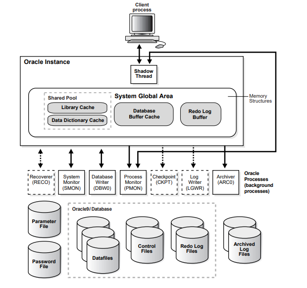
Oracle $9 i$ database is not a typical Windows process. On Windows, an Oracle instance (threads and memory structures) is a Windows service: a background process registered with the operating system. The service is started by Windows and requires no user interaction to start. This enables the database to open automatically at startup.
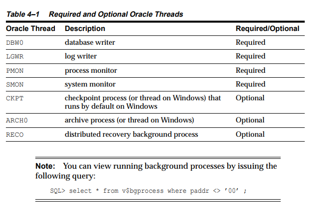
When running multiple Oracle instances on Windows, each instance runs its own Windows service with multiple component threads. Each thread may be required for the database to be available, or it may be optional and specific to certain platforms. Examples of optional and required threads on Windows are listed in Table 4-1.

计算机代写|数据库作业代写Database代考|File I/O Enhancements

Oracle $9 i$ database supports 64 -bit file $\mathrm{I} / \mathrm{O}$ to allow use of files larger than 4 gigabytes (GB) in size. In addition, physical and logical raw files are supported as data, log, and control files to support Oracle Real Application Clusters on Windows and for those cases where performance needs to be maximized.

All Oracle $9 i$ file $\mathrm{I} / \mathrm{O}$ routines support 64 -bit file offsets, meaning there are no $2 \mathrm{~GB}$ or 4 GB file size limitations when it comes to data, log, or control files, as there are on some other platforms. In fact, the limitations that are in place are generic Oracle limitations across all platforms. These limits include 4 million database blocks for each file, $16 \mathrm{~KB}$ maximum block size, and $64 \mathrm{~K}$ files for each database. If these values are multiplied, then maximum file size for a database file on Windows is 64 GB, and maximum total database size supported (with $16 \mathrm{~KB}$ database blocks) is 4 petabytes.
Raw File Support
Windows supports raw files, similar to UNIX. Using raw files for database or log files can have a slight performance gain. Raw files are unformatted disk partitions that can be used as one large file. Raw files have the benefit of no file system overhead, because they are unformatted partitions. However, standard Windows commands do not support manipulating or backing up raw files. As a result, raw files are generally used only by very high-end installations and by Oracle Real Application Clusters, where they are required.
To Oracle $9 i$, raw files are no different from other Oracle $9 i$ database files. They are treated in the same way by Oracle as any other file and can be backed up and restored through Recovery Manager or OCOPY.

计算机代写|数据库作业代写Database代考|INFS3200

数据库代考

机代写|数据库作业代写Database代考|Oracle9i on Windows Architecture

Windows上的Oracle $ 9i $是一个稳定、可靠和高性能的系统,可以在其上构建应用程序。数据库的每个版本都为Windows上的高性能提供了新的特定于平台的特性。
Oracle $ 9i $在Windows和其他平台上的操作方式相同。该架构在Windows上提供了几个优势,例如:

用基于线程的架构

文件I/O增强

原始文件支持
用基于线程的架构
Oracle $ 9i $数据库的内部进程架构是基于线程的。线程是进程中运行程序指令的对象。线程允许进程内的并发操作,这样进程就可以在不同的处理器上同时运行程序的不同部分。基于线程的架构提供了以下优点:

更快的上下文切换

更简单的系统全局区域分配例程,因为它不需要使用共享内存

生成新连接的速度更快,因为线程的创建速度比进程快

减少内存使用,因为线程比进程共享更多的数据结构

在内部,实现线程模型的代码是紧凑的,并且与Oracle代码的主体分离。异常处理程序和例程跟踪和取消分配资源。它们增加了健壮性,不会因为资源泄漏或程序行为不当而停机。
Oracle $ 9i $数据库不是典型的Windows进程。在Windows上,Oracle实例(线程和内存结构)是一个Windows服务:一个注册在操作系统上的后台进程。该服务由Windows启动,不需要用户交互即可启动。这使数据库能够在启动时自动打开。
当在Windows上运行多个Oracle实例时,每个实例使用多个组件线程运行自己的Windows服务。每个线程可能是数据库可用所必需的,也可能是可选的,特定于某些平台。Windows上可选和必选线程的示例如表4-1所示。

计算机代写|数据库作业代写Database代考|File I/O Enhancements

Oracle $ 9i $ database支持64位文件$\mathrm{i} / \mathrm{O}$,允许使用大于4gb的文件。此外,支持物理和逻辑原始文件作为数据、日志和控制文件,以支持Windows上的Oracle Real Application Clusters和那些需要最大化性能的情况。

所有Oracle $ 9i $ file $\mathrm{i} / \mathrm{O}$例程都支持64位文件偏移量,这意味着当涉及到数据、日志或控制文件时,不存在$2 \mathrm{~GB}$或4gb文件大小的限制,而在其他一些平台上存在这些限制。实际上,存在的限制是所有平台上通用的Oracle限制。这些限制包括每个文件400万个数据库块,最大块大小$16 \mathrm{~KB}$,每个数据库$64 \mathrm{~K}$文件。如果将这些值相乘,则Windows上数据库文件的最大文件大小为64gb,支持的最大数据库总大小(使用$16 \ mathm {~KB}$数据库块)为4pb。
原始文件支持
Windows支持原始文件,类似于UNIX。使用原始文件作为数据库或日志文件可以略微提高性能。原始文件是未格式化的磁盘分区,可以用作一个大文件。原始文件的好处是没有文件系统开销,因为它们是未格式化的分区。但是,标准的Windows命令不支持操作或备份原始文件。因此,原始文件通常只在非常高端的安装和Oracle真实应用程序集群中使用。
对于Oracle $ 9i $,原始文件与其他Oracle $ 9i $数据库文件没有什么不同。Oracle对它们的处理方式与其他文件相同,可以通过恢复管理器或OCOPY进行备份和恢复。

计算机代写|数据库作业代写Database代考 请认准statistics-lab™

统计代写请认准statistics-lab™. statistics-lab™为您的留学生涯保驾护航。

金融工程代写

金融工程是使用数学技术来解决金融问题。金融工程使用计算机科学、统计学、经济学和应用数学领域的工具和知识来解决当前的金融问题,以及设计新的和创新的金融产品。

非参数统计代写

非参数统计指的是一种统计方法,其中不假设数据来自于由少数参数决定的规定模型;这种模型的例子包括正态分布模型和线性回归模型。

广义线性模型代考

广义线性模型(GLM)归属统计学领域,是一种应用灵活的线性回归模型。该模型允许因变量的偏差分布有除了正态分布之外的其它分布。

术语 广义线性模型(GLM)通常是指给定连续和/或分类预测因素的连续响应变量的常规线性回归模型。它包括多元线性回归,以及方差分析和方差分析(仅含固定效应)。

有限元方法代写

有限元方法(FEM)是一种流行的方法,用于数值解决工程和数学建模中出现的微分方程。典型的问题领域包括结构分析、传热、流体流动、质量运输和电磁势等传统领域。

有限元是一种通用的数值方法,用于解决两个或三个空间变量的偏微分方程(即一些边界值问题)。为了解决一个问题,有限元将一个大系统细分为更小、更简单的部分,称为有限元。这是通过在空间维度上的特定空间离散化来实现的,它是通过构建对象的网格来实现的:用于求解的数值域,它有有限数量的点。边界值问题的有限元方法表述最终导致一个代数方程组。该方法在域上对未知函数进行逼近。[1] 然后将模拟这些有限元的简单方程组合成一个更大的方程系统,以模拟整个问题。然后,有限元通过变化微积分使相关的误差函数最小化来逼近一个解决方案。

tatistics-lab作为专业的留学生服务机构,多年来已为美国、英国、加拿大、澳洲等留学热门地的学生提供专业的学术服务,包括但不限于Essay代写,Assignment代写,Dissertation代写,Report代写,小组作业代写,Proposal代写,Paper代写,Presentation代写,计算机作业代写,论文修改和润色,网课代做,exam代考等等。写作范围涵盖高中,本科,研究生等海外留学全阶段,辐射金融,经济学,会计学,审计学,管理学等全球99%专业科目。写作团队既有专业英语母语作者,也有海外名校硕博留学生,每位写作老师都拥有过硬的语言能力,专业的学科背景和学术写作经验。我们承诺100%原创,100%专业,100%准时,100%满意。

随机分析代写


随机微积分是数学的一个分支,对随机过程进行操作。它允许为随机过程的积分定义一个关于随机过程的一致的积分理论。这个领域是由日本数学家伊藤清在第二次世界大战期间创建并开始的。

时间序列分析代写

随机过程,是依赖于参数的一组随机变量的全体,参数通常是时间。 随机变量是随机现象的数量表现,其时间序列是一组按照时间发生先后顺序进行排列的数据点序列。通常一组时间序列的时间间隔为一恒定值(如1秒,5分钟,12小时,7天,1年),因此时间序列可以作为离散时间数据进行分析处理。研究时间序列数据的意义在于现实中,往往需要研究某个事物其随时间发展变化的规律。这就需要通过研究该事物过去发展的历史记录,以得到其自身发展的规律。

回归分析代写

多元回归分析渐进(Multiple Regression Analysis Asymptotics)属于计量经济学领域,主要是一种数学上的统计分析方法,可以分析复杂情况下各影响因素的数学关系,在自然科学、社会和经济学等多个领域内应用广泛。

MATLAB代写

MATLAB 是一种用于技术计算的高性能语言。它将计算、可视化和编程集成在一个易于使用的环境中,其中问题和解决方案以熟悉的数学符号表示。典型用途包括:数学和计算算法开发建模、仿真和原型制作数据分析、探索和可视化科学和工程图形应用程序开发,包括图形用户界面构建MATLAB 是一个交互式系统,其基本数据元素是一个不需要维度的数组。这使您可以解决许多技术计算问题,尤其是那些具有矩阵和向量公式的问题,而只需用 C 或 Fortran 等标量非交互式语言编写程序所需的时间的一小部分。MATLAB 名称代表矩阵实验室。MATLAB 最初的编写目的是提供对由 LINPACK 和 EISPACK 项目开发的矩阵软件的轻松访问,这两个项目共同代表了矩阵计算软件的最新技术。MATLAB 经过多年的发展,得到了许多用户的投入。在大学环境中,它是数学、工程和科学入门和高级课程的标准教学工具。在工业领域,MATLAB 是高效研究、开发和分析的首选工具。MATLAB 具有一系列称为工具箱的特定于应用程序的解决方案。对于大多数 MATLAB 用户来说非常重要,工具箱允许您学习应用专业技术。工具箱是 MATLAB 函数(M 文件)的综合集合,可扩展 MATLAB 环境以解决特定类别的问题。可用工具箱的领域包括信号处理、控制系统、神经网络、模糊逻辑、小波、仿真等。

R语言代写问卷设计与分析代写
PYTHON代写回归分析与线性模型代写
MATLAB代写方差分析与试验设计代写
STATA代写机器学习/统计学习代写
SPSS代写计量经济学代写
EVIEWS代写时间序列分析代写
EXCEL代写深度学习代写
SQL代写各种数据建模与可视化代写

计算机代写|数据库作业代写Database代考|INFS3200

如果你也在 怎样代写数据库Database 这个学科遇到相关的难题,请随时右上角联系我们的24/7代写客服。数据库Database可以成为一种强大的工具,它可以做计算机程序最擅长的事情:存储、操作和显示数据。

数据库Database不仅在许多应用程序中发挥作用,而且经常发挥关键作用。如果数据没有正确存储,它可能会损坏,程序将无法有意义地使用它。如果数据组织不当,程序可能无法在合理的时间内找到所需的数据。
除非数据库安全有效地存储其数据,否则无论系统的其余部分设计得多么好,应用程序都将是无用的。

statistics-lab™ 为您的留学生涯保驾护航 在代写数据库Database方面已经树立了自己的口碑, 保证靠谱, 高质且原创的统计Statistics代写服务。我们的专家在代写数据库Database代写方面经验极为丰富,各种代写数据库Database相关的作业也就用不着说。

计算机代写|数据库作业代写Database代考|INFS3200

计算机代写|数据库作业代写Database代考|Install Accounts and Groups

UNIX uses the concept of a DBA group. The root account cannot be used to install Oracle. A separate Oracle account must be created manually.
On Windows, Oracle must be installed by a Windows username in the Administrators group. The username is automatically added to the Windows local group $O R A$ _ DBA, which receives the SYSDBA privilege. This allows the user to log in to the database using CONNECT / AS SYSDBA and not be prompted for a password.

Password files are located in the ORACLE_BASE\ORACLE_HOME\database directory and are named pwdSID. ora, where SID identifies the Oracle $9 i$ database instance.

Installation
The following manual setup tasks, all required on UNIX, are not required on Windows:

Set environment variables

Create a DBA group for database administrators

Create a group for users running Oracle Universal Installer

Create an account dedicated to installing and upgrading Oracle componentsMemory Resources
The resources provided by the UNIX default kernels are often inadequate for a medium or large Oracle database. The maximum size of a shared memory segment (SHMMAX) and maximum number of semaphores available (SEMMNS) may be too low for Oracle recommendations.

On Windows, fewer resources are needed for interprocess communication (IPC), because the Oracle relational database management system is thread-based and not process-based. These resources, including shared memory and semaphores, are not adjustable by the user.

计算机代写|数据库作业代写Database代考|Milcrosoft Iransaction server

UNIX does not support Microsoft Transaction Server.
Windows supports Microsoft Transaction Server beginning with Oracle version 8 . Using ORACLEMTSRecoveryService, you can develop and deploy applications based on COM/COM+. Microsoft Transaction Server coordinates application transactions for an Oracle database.


Multiple Oracle Homes and OFA
The goal of OFA is to place all Oracle software under one ORACLE_BASE directory and to spread database files across different physical drives as databases increase in size. OFA is implemented on Windows NT and UNIX in the same way, and main subdirectory and filenames are the same on both operating systems. Windows NT and Unix differ, however, in their OFA directory tree top-level names and in the way variables are set.

On UNIX, ORACLE_BASE is associated with a user’s environment. ORACLE_HOME and ORACLE_SID must be set in system or user login scripts. Symbolic links are supported. Although everything seems to be in one directory on the same hard drive, files may be on different hard drives if they are symbolically linked or have that directory as a mount point.
On Windows, ORACLE_BASE is defined in the registry (for example, in HKEY LOCAL_MACHINE \SOFTWARE \ORACLE \HOMEO). ORACLE_HOME and ORACLE_SID are variables defined in the registry. Symbolic links like those on UNIX are not

Processes and Threads
On UNIX, Oracle uses a process to implement each of such background tasks as database writer (DBWO), log writer (LGWR), shared server process dispatchers, and shared servers. Each dedicated connection made to the database causes another operating system process to be spawned on behalf of that session.
On Windows, each background process is implemented as a thread inside a single, large process. For each Oracle database instance or system identifier, there is one corresponding process for Oracle $9 i$ database. For example, 100 Oracle processes for a database instance on UNIX are handled by 100 threads inside one process on Windows.

All Oracle background, dedicated server, and client processes are threads of the master ORACLE Windows process, and all threads of the ORACLE process share resources. This multithreaded architecture is highly efficient, allowing fast context switches with low overhead.

To view processes or end individual threads, use Oracle Administration Assistant for Windows NT. Choose Start > Programs > Oracle – HOME_NAME > Configuration and Migration Tools > Administration Assistant for Windows. Right-click the SID and choose Process Information.

计算机代写|数据库作业代写Database代考|INFS3200

数据库代考

计算机代写|数据库作业代写Database代考|Install Accounts and Groups

UNIX使用DBA组的概念。不能使用root帐号安装Oracle。必须手动创建一个单独的Oracle帐户。
在Windows操作系统下,Oracle必须以Administrators组中的Windows用户名安装。该用户名被自动添加到Windows本地组$O R A$ _ DBA中,该组具有SYSDBA权限。这允许用户使用CONNECT / AS SYSDBA登录到数据库,而不需要提示输入密码。

密码文件位于ORACLE_BASE\ORACLE_HOME\database目录下,命名为pwdSID。其中SID标识Oracle $ 9i $数据库实例。

安装
以下手动设置任务在UNIX上都是必需的,在Windows上则不需要:

设置环境变量

为数据库管理员创建DBA组

为运行Oracle通用安装程序的用户创建一个组

创建专门用于安装和升级Oracle组件的帐户

内存资源
UNIX默认内核提供的资源通常不足以用于中型或大型Oracle数据库。共享内存段的最大大小(SHMMAX)和可用信号量的最大数量(SEMMNS)可能低于Oracle的推荐值。

在Windows上,进程间通信(IPC)所需的资源更少,因为Oracle关系数据库管理系统是基于线程的,而不是基于进程的。这些资源,包括共享内存和信号量,是用户无法调整的。

计算机代写|数据库作业代写Database代考|Milcrosoft Iransaction server

UNIX不支持Microsoft Transaction Server。
Windows从Oracle version 8开始支持Microsoft Transaction Server。使用ORACLEMTSRecoveryService,您可以基于COM/COM+开发和部署应用程序。Microsoft Transaction Server为Oracle数据库协调应用程序事务。

多个Oracle Homes和OFA
OFA的目标是将所有Oracle软件放在一个ORACLE_BASE目录下,并随着数据库大小的增加将数据库文件分散到不同的物理驱动器上。OFA以相同的方式在Windows NT和UNIX上实现,主子目录和文件名在这两个操作系统上是相同的。但是,Windows NT和Unix的不同之处在于它们的OFA目录树顶级名称和设置变量的方式。

在UNIX上,ORACLE_BASE与用户的环境相关联。“ORACLE_HOME”和“ORACLE_SID”必须在系统或用户登录脚本中设置。支持符号链接。虽然所有内容似乎都在同一个硬盘驱动器上的一个目录中,但如果文件被符号链接或将该目录作为挂载点,则文件可能位于不同的硬盘驱动器上。
在Windows上,ORACLE_BASE是在注册表中定义的(例如,在HKEY LOCAL_MACHINE \SOFTWARE \ORACLE \HOMEO)。ORACLE_HOME和ORACLE_SID是在注册表中定义的变量。像UNIX上的符号链接不是

进程和线程
在UNIX上,Oracle使用一个进程来实现每个后台任务,如数据库写入器(DBWO)、日志写入器(LGWR)、共享服务器进程调度器和共享服务器。与数据库建立的每个专用连接都会导致为该会话生成另一个操作系统进程。
在Windows上,每个后台进程都是作为单个大进程中的线程实现的。对于每个Oracle数据库实例或系统标识符,都有一个对应的Oracle $ 9i $ database进程。例如,UNIX上一个数据库实例的100个Oracle进程在Windows上由一个进程内的100个线程处理。

所有Oracle后台进程、专用服务器进程和客户端进程都是Oracle Windows主进程的线程,所有Oracle进程的线程共享资源。这种多线程体系结构非常高效,允许以低开销进行快速上下文切换。

要查看进程或结束单个线程,请使用Windows NT的Oracle Administration Assistant。选择“开始>程序> Oracle – HOME_NAME >配置和迁移工具> Windows的Administration Assistant”。右键单击SID并选择Process Information。

计算机代写|数据库作业代写Database代考 请认准statistics-lab™

统计代写请认准statistics-lab™. statistics-lab™为您的留学生涯保驾护航。

金融工程代写

金融工程是使用数学技术来解决金融问题。金融工程使用计算机科学、统计学、经济学和应用数学领域的工具和知识来解决当前的金融问题,以及设计新的和创新的金融产品。

非参数统计代写

非参数统计指的是一种统计方法,其中不假设数据来自于由少数参数决定的规定模型;这种模型的例子包括正态分布模型和线性回归模型。

广义线性模型代考

广义线性模型(GLM)归属统计学领域,是一种应用灵活的线性回归模型。该模型允许因变量的偏差分布有除了正态分布之外的其它分布。

术语 广义线性模型(GLM)通常是指给定连续和/或分类预测因素的连续响应变量的常规线性回归模型。它包括多元线性回归,以及方差分析和方差分析(仅含固定效应)。

有限元方法代写

有限元方法(FEM)是一种流行的方法,用于数值解决工程和数学建模中出现的微分方程。典型的问题领域包括结构分析、传热、流体流动、质量运输和电磁势等传统领域。

有限元是一种通用的数值方法,用于解决两个或三个空间变量的偏微分方程(即一些边界值问题)。为了解决一个问题,有限元将一个大系统细分为更小、更简单的部分,称为有限元。这是通过在空间维度上的特定空间离散化来实现的,它是通过构建对象的网格来实现的:用于求解的数值域,它有有限数量的点。边界值问题的有限元方法表述最终导致一个代数方程组。该方法在域上对未知函数进行逼近。[1] 然后将模拟这些有限元的简单方程组合成一个更大的方程系统,以模拟整个问题。然后,有限元通过变化微积分使相关的误差函数最小化来逼近一个解决方案。

tatistics-lab作为专业的留学生服务机构,多年来已为美国、英国、加拿大、澳洲等留学热门地的学生提供专业的学术服务,包括但不限于Essay代写,Assignment代写,Dissertation代写,Report代写,小组作业代写,Proposal代写,Paper代写,Presentation代写,计算机作业代写,论文修改和润色,网课代做,exam代考等等。写作范围涵盖高中,本科,研究生等海外留学全阶段,辐射金融,经济学,会计学,审计学,管理学等全球99%专业科目。写作团队既有专业英语母语作者,也有海外名校硕博留学生,每位写作老师都拥有过硬的语言能力,专业的学科背景和学术写作经验。我们承诺100%原创,100%专业,100%准时,100%满意。

随机分析代写


随机微积分是数学的一个分支,对随机过程进行操作。它允许为随机过程的积分定义一个关于随机过程的一致的积分理论。这个领域是由日本数学家伊藤清在第二次世界大战期间创建并开始的。

时间序列分析代写

随机过程,是依赖于参数的一组随机变量的全体,参数通常是时间。 随机变量是随机现象的数量表现,其时间序列是一组按照时间发生先后顺序进行排列的数据点序列。通常一组时间序列的时间间隔为一恒定值(如1秒,5分钟,12小时,7天,1年),因此时间序列可以作为离散时间数据进行分析处理。研究时间序列数据的意义在于现实中,往往需要研究某个事物其随时间发展变化的规律。这就需要通过研究该事物过去发展的历史记录,以得到其自身发展的规律。

回归分析代写

多元回归分析渐进(Multiple Regression Analysis Asymptotics)属于计量经济学领域,主要是一种数学上的统计分析方法,可以分析复杂情况下各影响因素的数学关系,在自然科学、社会和经济学等多个领域内应用广泛。

MATLAB代写

MATLAB 是一种用于技术计算的高性能语言。它将计算、可视化和编程集成在一个易于使用的环境中,其中问题和解决方案以熟悉的数学符号表示。典型用途包括:数学和计算算法开发建模、仿真和原型制作数据分析、探索和可视化科学和工程图形应用程序开发,包括图形用户界面构建MATLAB 是一个交互式系统,其基本数据元素是一个不需要维度的数组。这使您可以解决许多技术计算问题,尤其是那些具有矩阵和向量公式的问题,而只需用 C 或 Fortran 等标量非交互式语言编写程序所需的时间的一小部分。MATLAB 名称代表矩阵实验室。MATLAB 最初的编写目的是提供对由 LINPACK 和 EISPACK 项目开发的矩阵软件的轻松访问,这两个项目共同代表了矩阵计算软件的最新技术。MATLAB 经过多年的发展,得到了许多用户的投入。在大学环境中,它是数学、工程和科学入门和高级课程的标准教学工具。在工业领域,MATLAB 是高效研究、开发和分析的首选工具。MATLAB 具有一系列称为工具箱的特定于应用程序的解决方案。对于大多数 MATLAB 用户来说非常重要,工具箱允许您学习应用专业技术。工具箱是 MATLAB 函数(M 文件)的综合集合,可扩展 MATLAB 环境以解决特定类别的问题。可用工具箱的领域包括信号处理、控制系统、神经网络、模糊逻辑、小波、仿真等。

R语言代写问卷设计与分析代写
PYTHON代写回归分析与线性模型代写
MATLAB代写方差分析与试验设计代写
STATA代写机器学习/统计学习代写
SPSS代写计量经济学代写
EVIEWS代写时间序列分析代写
EXCEL代写深度学习代写
SQL代写各种数据建模与可视化代写

计算机代写|机器学习代写machine learning代考|COMP3308

如果你也在 怎样代写机器学习Machine Learning 这个学科遇到相关的难题,请随时右上角联系我们的24/7代写客服。机器学习Machine Learning令人兴奋。这是有趣的,具有挑战性的,创造性的,和智力刺激。它还为公司赚钱,自主处理大量任务,并从那些宁愿做其他事情的人那里消除单调工作的繁重任务。

机器学习Machine Learning也非常复杂。从数千种算法、数百种开放源码包,以及需要具备从数据工程(DE)到高级统计分析和可视化等各种技能的专业实践者,ML专业实践者所需的工作确实令人生畏。增加这种复杂性的是,需要能够与广泛的专家、主题专家(sme)和业务单元组进行跨功能工作——就正在解决的问题的性质和ml支持的解决方案的输出进行沟通和协作。

statistics-lab™ 为您的留学生涯保驾护航 在代写机器学习 machine learning方面已经树立了自己的口碑, 保证靠谱, 高质且原创的统计Statistics代写服务。我们的专家在代写机器学习 machine learning代写方面经验极为丰富,各种代写机器学习 machine learning相关的作业也就用不着说。

计算机代写|机器学习代写machine learning代考|COMP3308

计算机代写|机器学习代写machine learning代考|Bias and Variance Analysis

Bias and variance analysis plays an important role in ensemble classification research due to the framework it provides for classifier prediction error decomposition.

Initially, Geman has decomposed prediction error into bias and variance terms under the regression setting using squared-error loss [10]. This decomposition brings about the fact that a decrease/increase in the prediction error rate is caused by a decrease/increase in bias, or in variance, or in both. Extensions of the analysis have been carried out on the classification setting, and later applied on different ensemble classifiers in order to analyse the reason behind their success over single classifiers. It has been shown that the reason for most of the ensembles to have lower prediction error rates is due to the reductions they offer in sense of both bias and variance.
However, the extension of the original theoretical analysis on regression has been done in various ways by different researchers for classification; and there is no standard definition accepted. Therefore, the results of the analyses also differ from each other slightly. Some of the definitions/frameworks that have gained interest within the research field are given by Breiman [3], Kohavi and Wolpert [15], Dietterich and Kong [16], Friedman [9], Wolpert [25], Heskes [11], Tibshirani [19], Domingos [6] and James [13].

Although there are dissimilarities in-between the frameworks, the main intuitions behind each are similar. Consider a training set $T$ with patterns $\left(x_i, l_i\right)$, where $x$ represents the feature vector and $l$ the corresponding label. Given a test pattern, an optimal classifier model predicts a decision label by assuring the lowest expected loss over all possible target label values. This classifier, which is actually the Bayes classifier when used with the zero-one loss function, is supposed to know and use the underlying likelihood probability distribution for the input dataset patterns/classes. If we call the decision of the optimal classifier as the optimal decision $(O D)$, then for a given test pattern $\left(x_i, l_i\right), O D=\operatorname{argmin}_\alpha E_t[L(t, \alpha)]$ where $L$ denotes the loss function used, and $l$ the possible target label values.

The estimator, on the other hand, is actually an averaged classifier model. It predicts a decision label by assuring the lowest expected loss over all labels that are created by classifiers trained on different training sets. The intrinsic parameters of these classifiers are usually the same, and the only difference is the training sets that they are trained on. In this case, instead of minimizing the loss over the target labels using the known underlying probability distribution as happens in the optimal classifier case, the minimization of the loss is carried out for the set of labels which are created by the classifiers trained on various training sets. If the decision of the estimator is named as the expected estimator decision $(E E D)$; then for a given test pattern $\left(x_i, l_i\right), E E D=\operatorname{argmin}_\alpha E_l[L(l, \alpha)]$ where $L$ denotes the loss function used, and $l$ the label values obtained from the classifiers used. For regression under the squared-error loss setting, the $O D$ is the mean of the target labels while the EED is the mean of the classifier decisions obtained via different training sets.

计算机代写|机器学习代写machine learning代考|Bias and Variance Analysis of James

James [13] extends the prediction error decomposition, which is initially proposed by Geman et al [10] for squared error under regression setting, for all symmetric loss functions. Therefore, his definition also covers zero-one loss under classification setting, which we use in the experiments.

In his decomposition, the terms systematic effect (SE) and variance effect (VE) satisfy the additive decomposition for all symmetric loss functions, and for both real valued and categorical predictors. They actually indicate the effect of bias and variance on the prediction error. For example, a negative $V E$ would mean that variance actually helps reduce the prediction error. On the other hand, the bias term is defined to show the average distance between the response and the predictor; and the variance term refers to the variability of the predictor. As a result, both the meanings and the additive characteristics of the bias and variance concepts of the original setup have been preserved. Following is a summary of the bias-variance derivations of James:

For any symmetric loss function $L$, where $L(a, b)=L(b, a)$ :
$$
\begin{aligned}
E_{Y, \tilde{Y}}[L(Y, \tilde{Y})]= & E_Y[L(Y, S Y)]+E_Y[L(Y, S \tilde{Y})-L(Y, S Y)] \
& +E_{Y, \tilde{Y}}[L(Y, \tilde{Y})-L(Y, S \tilde{Y})] \
\text { predictionerror }= & \operatorname{Var}(Y)+S E(\tilde{Y}, Y)+\operatorname{VE}(\tilde{Y}, Y)
\end{aligned}
$$
where $L(a, b)$ is the loss when $b$ is used in predicting $a, Y$ is the response and $\tilde{Y}$ is the predictor. $S Y=\operatorname{argmin}\mu E_Y[L(Y, \mu)]$ and $S \tilde{Y}=\operatorname{argmin}\mu E_Y[L(\tilde{Y}, \mu)]$. We see here that prediction error is composed of the variance of the response (irreducible noise), $S E$ and $V E$.

Using the same terminology, the bias and variance for the predictor are defined as follows:
$$
\begin{aligned}
\operatorname{Bias}(\tilde{Y}) & =L(S Y, S \tilde{Y}) \
\operatorname{Var}(\tilde{Y}) & =E_{\tilde{Y}}[L(\tilde{Y}, S \tilde{Y})]
\end{aligned}
$$
When the specific case of classification problems with zero-one loss function is considered, we end up with the following formulations:
$L(a, b)=I(a \neq b), Y \varepsilon{1,2,3 . . N}$ for an $N$ class problem, $P_i^Y=P_Y(Y=i), P_i^{\tilde{Y}}=$ $P_{\tilde{Y}}(\tilde{Y}=i), S T=\operatorname{argmin}i E_Y[I(Y \neq i)]=\operatorname{argmax}_i P_i^Y$ Therefore, $$ \begin{aligned} \operatorname{Var}(Y) & =P_Y(Y \neq S Y)=1-\max _i P_i^Y \ \operatorname{Var}(\tilde{Y}) & =P{\tilde{Y}}(\tilde{Y} \neq S \tilde{Y})=1-\max i P_i^{\tilde{Y}} \ \operatorname{Bias}(\tilde{Y}) & =I(S \tilde{Y} \neq S Y) \ \operatorname{VE}(\tilde{Y}, Y) & =P(Y \neq \tilde{Y})-P_Y(Y \neq S \tilde{Y})=P{S \tilde{Y}}^Y-\sum_i P_i^Y P_i^{\tilde{Y}} \
S E(\tilde{Y}, Y) & =P_Y(Y \neq S \tilde{Y})-P_Y(Y \neq S Y)=P_{S Y}^Y-P_{S \tilde{Y}}^Y
\end{aligned}
$$
where $I(q)$ is 1 if $q$ is a true argument and 0 otherwise.

计算机代写|机器学习代写machine learning代考|COMP3308

机器学习代考

计算机代写|机器学习代写machine learning代考|Bias and Variance Analysis

偏差和方差分析为分类器预测误差分解提供了框架,在集成分类研究中起着重要的作用。

最初,german使用误差平方损失将回归设置下的预测误差分解为偏差项和方差项[10]。这种分解带来的事实是,预测错误率的减少/增加是由偏差或方差的减少/增加引起的,或者两者兼而有之。本文对分类设置进行了扩展分析,随后将其应用于不同的集成分类器,以分析它们优于单一分类器的原因。已经表明,大多数集成具有较低的预测错误率的原因是由于它们在偏差和方差的意义上提供了减少。
然而,不同的研究人员以不同的方式对回归的原始理论分析进行了扩展,用于分类;目前还没有公认的标准定义。因此,分析结果也略有不同。Breiman[3]、Kohavi and Wolpert[15]、Dietterich and Kong[16]、Friedman[9]、Wolpert[25]、Heskes[11]、Tibshirani[19]、Domingos[6]和James[13]给出了一些在研究领域引起兴趣的定义/框架。

尽管框架之间存在差异,但每个框架背后的主要直觉是相似的。考虑一个模式为$\left(x_i, l_i\right)$的训练集$T$,其中$x$表示特征向量,$l$表示相应的标签。给定一个测试模式,最优分类器模型通过确保所有可能的目标标签值的最低预期损失来预测决策标签。当与0 – 1损失函数一起使用时,这个分类器实际上是贝叶斯分类器,它应该知道并使用输入数据集模式/类的潜在可能性概率分布。如果我们将最优分类器的决策称为最优决策$(O D)$,那么对于给定的测试模式$\left(x_i, l_i\right), O D=\operatorname{argmin}_\alpha E_t[L(t, \alpha)]$,其中$L$表示使用的损失函数,$l$表示可能的目标标签值。

另一方面,估计器实际上是一个平均分类器模型。它通过确保在不同训练集上训练的分类器创建的所有标签上的最低预期损失来预测决策标签。这些分类器的内在参数通常是相同的,唯一的区别是它们所训练的训练集。在这种情况下,与在最优分类器情况下使用已知的潜在概率分布最小化目标标签上的损失不同,对由在各种训练集上训练的分类器创建的标签集进行最小化损失。如果估计器的决策被命名为预期估计器决策$(E E D)$;然后对于给定的测试模式$\left(x_i, l_i\right), E E D=\operatorname{argmin}_\alpha E_l[L(l, \alpha)]$,其中$L$表示使用的损失函数,$l$表示从使用的分类器获得的标签值。对于平方误差损失设置下的回归,$O D$为目标标签的均值,EED为通过不同训练集得到的分类器决策的均值。

计算机代写|机器学习代写machine learning代考|Bias and Variance Analysis of James

James[13]将Geman等[10]最初针对回归设置下的平方误差提出的预测误差分解扩展到所有对称损失函数。因此,他的定义也涵盖了我们在实验中使用的分类设置下的0 – 1损失。

在他的分解中,系统效应(SE)和方差效应(VE)两项满足所有对称损失函数的加性分解,对于实值和分类预测器都是如此。它们实际上表明了偏差和方差对预测误差的影响。例如,负值$V E$意味着方差实际上有助于减少预测误差。另一方面,定义偏差项来表示响应和预测器之间的平均距离;方差项指的是预测器的可变性。结果,保留了原始设置的偏差和方差概念的含义和可加性特征。下面是James的偏方差推导的总结:

对于任意对称损失函数$L$,其中$L(a, b)=L(b, a)$:
$$
\begin{aligned}
E_{Y, \tilde{Y}}[L(Y, \tilde{Y})]= & E_Y[L(Y, S Y)]+E_Y[L(Y, S \tilde{Y})-L(Y, S Y)] \
& +E_{Y, \tilde{Y}}[L(Y, \tilde{Y})-L(Y, S \tilde{Y})] \
\text { predictionerror }= & \operatorname{Var}(Y)+S E(\tilde{Y}, Y)+\operatorname{VE}(\tilde{Y}, Y)
\end{aligned}
$$
当$b$用于预测时,$L(a, b)$是损失$a, Y$是响应,$\tilde{Y}$是预测者。$S Y=\operatorname{argmin}\mu E_Y[L(Y, \mu)]$和$S \tilde{Y}=\operatorname{argmin}\mu E_Y[L(\tilde{Y}, \mu)]$。我们在这里看到,预测误差由响应的方差(不可约噪声),$S E$和$V E$组成。

使用相同的术语,预测器的偏差和方差定义如下:
$$
\begin{aligned}
\operatorname{Bias}(\tilde{Y}) & =L(S Y, S \tilde{Y}) \
\operatorname{Var}(\tilde{Y}) & =E_{\tilde{Y}}[L(\tilde{Y}, S \tilde{Y})]
\end{aligned}
$$
当考虑具有0 – 1损失函数的分类问题的具体情况时,我们得到如下公式:
$L(a, b)=I(a \neq b), Y \varepsilon{1,2,3 . . N}$为$N$类问题,$P_i^Y=P_Y(Y=i), P_i^{\tilde{Y}}=$$P_{\tilde{Y}}(\tilde{Y}=i), S T=\operatorname{argmin}i E_Y[I(Y \neq i)]=\operatorname{argmax}i P_i^Y$因此,$$ \begin{aligned} \operatorname{Var}(Y) & =P_Y(Y \neq S Y)=1-\max _i P_i^Y \ \operatorname{Var}(\tilde{Y}) & =P{\tilde{Y}}(\tilde{Y} \neq S \tilde{Y})=1-\max i P_i^{\tilde{Y}} \ \operatorname{Bias}(\tilde{Y}) & =I(S \tilde{Y} \neq S Y) \ \operatorname{VE}(\tilde{Y}, Y) & =P(Y \neq \tilde{Y})-P_Y(Y \neq S \tilde{Y})=P{S \tilde{Y}}^Y-\sum_i P_i^Y P_i^{\tilde{Y}} \ S E(\tilde{Y}, Y) & =P_Y(Y \neq S \tilde{Y})-P_Y(Y \neq S Y)=P{S Y}^Y-P_{S \tilde{Y}}^Y
\end{aligned}
$$
如果$q$为真参数,$I(q)$为1,否则为0。

计算机代写|机器学习代写machine learning代考 请认准statistics-lab™

统计代写请认准statistics-lab™. statistics-lab™为您的留学生涯保驾护航。

金融工程代写

金融工程是使用数学技术来解决金融问题。金融工程使用计算机科学、统计学、经济学和应用数学领域的工具和知识来解决当前的金融问题,以及设计新的和创新的金融产品。

非参数统计代写

非参数统计指的是一种统计方法,其中不假设数据来自于由少数参数决定的规定模型;这种模型的例子包括正态分布模型和线性回归模型。

广义线性模型代考

广义线性模型(GLM)归属统计学领域,是一种应用灵活的线性回归模型。该模型允许因变量的偏差分布有除了正态分布之外的其它分布。

术语 广义线性模型(GLM)通常是指给定连续和/或分类预测因素的连续响应变量的常规线性回归模型。它包括多元线性回归,以及方差分析和方差分析(仅含固定效应)。

有限元方法代写

有限元方法(FEM)是一种流行的方法,用于数值解决工程和数学建模中出现的微分方程。典型的问题领域包括结构分析、传热、流体流动、质量运输和电磁势等传统领域。

有限元是一种通用的数值方法,用于解决两个或三个空间变量的偏微分方程(即一些边界值问题)。为了解决一个问题,有限元将一个大系统细分为更小、更简单的部分,称为有限元。这是通过在空间维度上的特定空间离散化来实现的,它是通过构建对象的网格来实现的:用于求解的数值域,它有有限数量的点。边界值问题的有限元方法表述最终导致一个代数方程组。该方法在域上对未知函数进行逼近。[1] 然后将模拟这些有限元的简单方程组合成一个更大的方程系统,以模拟整个问题。然后,有限元通过变化微积分使相关的误差函数最小化来逼近一个解决方案。

tatistics-lab作为专业的留学生服务机构,多年来已为美国、英国、加拿大、澳洲等留学热门地的学生提供专业的学术服务,包括但不限于Essay代写,Assignment代写,Dissertation代写,Report代写,小组作业代写,Proposal代写,Paper代写,Presentation代写,计算机作业代写,论文修改和润色,网课代做,exam代考等等。写作范围涵盖高中,本科,研究生等海外留学全阶段,辐射金融,经济学,会计学,审计学,管理学等全球99%专业科目。写作团队既有专业英语母语作者,也有海外名校硕博留学生,每位写作老师都拥有过硬的语言能力,专业的学科背景和学术写作经验。我们承诺100%原创,100%专业,100%准时,100%满意。

随机分析代写


随机微积分是数学的一个分支,对随机过程进行操作。它允许为随机过程的积分定义一个关于随机过程的一致的积分理论。这个领域是由日本数学家伊藤清在第二次世界大战期间创建并开始的。

时间序列分析代写

随机过程,是依赖于参数的一组随机变量的全体,参数通常是时间。 随机变量是随机现象的数量表现,其时间序列是一组按照时间发生先后顺序进行排列的数据点序列。通常一组时间序列的时间间隔为一恒定值(如1秒,5分钟,12小时,7天,1年),因此时间序列可以作为离散时间数据进行分析处理。研究时间序列数据的意义在于现实中,往往需要研究某个事物其随时间发展变化的规律。这就需要通过研究该事物过去发展的历史记录,以得到其自身发展的规律。

回归分析代写

多元回归分析渐进(Multiple Regression Analysis Asymptotics)属于计量经济学领域,主要是一种数学上的统计分析方法,可以分析复杂情况下各影响因素的数学关系,在自然科学、社会和经济学等多个领域内应用广泛。

MATLAB代写

MATLAB 是一种用于技术计算的高性能语言。它将计算、可视化和编程集成在一个易于使用的环境中,其中问题和解决方案以熟悉的数学符号表示。典型用途包括:数学和计算算法开发建模、仿真和原型制作数据分析、探索和可视化科学和工程图形应用程序开发,包括图形用户界面构建MATLAB 是一个交互式系统,其基本数据元素是一个不需要维度的数组。这使您可以解决许多技术计算问题,尤其是那些具有矩阵和向量公式的问题,而只需用 C 或 Fortran 等标量非交互式语言编写程序所需的时间的一小部分。MATLAB 名称代表矩阵实验室。MATLAB 最初的编写目的是提供对由 LINPACK 和 EISPACK 项目开发的矩阵软件的轻松访问,这两个项目共同代表了矩阵计算软件的最新技术。MATLAB 经过多年的发展,得到了许多用户的投入。在大学环境中,它是数学、工程和科学入门和高级课程的标准教学工具。在工业领域,MATLAB 是高效研究、开发和分析的首选工具。MATLAB 具有一系列称为工具箱的特定于应用程序的解决方案。对于大多数 MATLAB 用户来说非常重要,工具箱允许您学习应用专业技术。工具箱是 MATLAB 函数(M 文件)的综合集合,可扩展 MATLAB 环境以解决特定类别的问题。可用工具箱的领域包括信号处理、控制系统、神经网络、模糊逻辑、小波、仿真等。

R语言代写问卷设计与分析代写
PYTHON代写回归分析与线性模型代写
MATLAB代写方差分析与试验设计代写
STATA代写机器学习/统计学习代写
SPSS代写计量经济学代写
EVIEWS代写时间序列分析代写
EXCEL代写深度学习代写
SQL代写各种数据建模与可视化代写

计算机代写|机器学习代写machine learning代考|QBUS6850

如果你也在 怎样代写机器学习Machine Learning 这个学科遇到相关的难题,请随时右上角联系我们的24/7代写客服。机器学习Machine Learning令人兴奋。这是有趣的,具有挑战性的,创造性的,和智力刺激。它还为公司赚钱,自主处理大量任务,并从那些宁愿做其他事情的人那里消除单调工作的繁重任务。

机器学习Machine Learning也非常复杂。从数千种算法、数百种开放源码包,以及需要具备从数据工程(DE)到高级统计分析和可视化等各种技能的专业实践者,ML专业实践者所需的工作确实令人生畏。增加这种复杂性的是,需要能够与广泛的专家、主题专家(sme)和业务单元组进行跨功能工作——就正在解决的问题的性质和ml支持的解决方案的输出进行沟通和协作。

statistics-lab™ 为您的留学生涯保驾护航 在代写机器学习 machine learning方面已经树立了自己的口碑, 保证靠谱, 高质且原创的统计Statistics代写服务。我们的专家在代写机器学习 machine learning代写方面经验极为丰富,各种代写机器学习 machine learning相关的作业也就用不着说。

计算机代写|机器学习代写machine learning代考|QBUS6850

计算机代写|机器学习代写machine learning代考|Error Correcting Output Coding (ECOC)

ECOC is an ensemble technique [4], in which multiple base classifiers are created and trained according to the information obtained from a pre-set binary code matrix. The main idea behind this procedure is to solve the original multi-class problem by combining the decision boundaries obtained from simpler two-class decompositions. The original problem is likely to be more complex compared to the subproblems into which it is decomposed, and therefore the aim is to come up with an easier and/or more accurate solution using the sub-problems rather than trying to solve it by a single complex classifier.

The base classifiers are actually two-class classifiers (dichotomizers), each of which is trained to solve a different bi-partitioning of the original problem. The bipartitions are created by combining the patterns from some predetermined classes together and relabeling them. An example bi-partitioning of an $N>2$ class dataset would be by having the patterns from the first 2 classes labeled as +1 and the last $N-2$ classes as -1 . The training patterns are therefore separated into two superclasses for each base classifier, and the information about how to create these superclasses is obtained from the ECOC matrix.

Consider an ECOC matrix $C$, where a particular element $C_{i j}$ is an element of the set $(+1,-1)$. Each $C_{i j}$ indicates the desired label for class $i$, to be used in training the base classifier $j$; and each row, called a codeword, represents the desired output for the whole set of base classifiers for the class it indicates. Figure 4.1 shows an ECOC matrix for a 4-class problem for illustration purposes.

计算机代写|机器学习代写machine learning代考|Bias and Variance Analysis

Bias and variance analysis plays an important role in ensemble classification research due to the framework it provides for classifier prediction error decomposition.

Initially, Geman has decomposed prediction error into bias and variance terms under the regression setting using squared-error loss [10]. This decomposition brings about the fact that a decrease/increase in the prediction error rate is caused by a decrease/increase in bias, or in variance, or in both. Extensions of the analysis have been carried out on the classification setting, and later applied on different ensemble classifiers in order to analyse the reason behind their success over single classifiers. It has been shown that the reason for most of the ensembles to have lower prediction error rates is due to the reductions they offer in sense of both bias and variance.
However, the extension of the original theoretical analysis on regression has been done in various ways by different researchers for classification; and there is no standard definition accepted. Therefore, the results of the analyses also differ from each other slightly. Some of the definitions/frameworks that have gained interest within the research field are given by Breiman [3], Kohavi and Wolpert [15], Dietterich and Kong [16], Friedman [9], Wolpert [25], Heskes [11], Tibshirani [19], Domingos [6] and James [13].

Although there are dissimilarities in-between the frameworks, the main intuitions behind each are similar. Consider a training set $T$ with patterns $\left(x_i, l_i\right)$, where $x$ represents the feature vector and $l$ the corresponding label. Given a test pattern, an optimal classifier model predicts a decision label by assuring the lowest expected loss over all possible target label values. This classifier, which is actually the Bayes classifier when used with the zero-one loss function, is supposed to know and use the underlying likelihood probability distribution for the input dataset patterns/classes. If we call the decision of the optimal classifier as the optimal decision $(O D)$, then for a given test pattern $\left(x_i, l_i\right), O D=\operatorname{argmin}_\alpha E_t[L(t, \alpha)]$ where $L$ denotes the loss function used, and $l$ the possible target label values.

The estimator, on the other hand, is actually an averaged classifier model. It predicts a decision label by assuring the lowest expected loss over all labels that are created by classifiers trained on different training sets. The intrinsic parameters of these classifiers are usually the same, and the only difference is the training sets that they are trained on. In this case, instead of minimizing the loss over the target labels using the known underlying probability distribution as happens in the optimal classifier case, the minimization of the loss is carried out for the set of labels which are created by the classifiers trained on various training sets. If the decision of the estimator is named as the expected estimator decision $(E E D)$; then for a given test pattern $\left(x_i, l_i\right), E E D=\operatorname{argmin}_\alpha E_l[L(l, \alpha)]$ where $L$ denotes the loss function used, and $l$ the label values obtained from the classifiers used. For regression under the squared-error loss setting, the $O D$ is the mean of the target labels while the $E E D$ is the mean of the classifier decisions obtained via different training sets.

计算机代写|机器学习代写machine learning代考|QBUS6850

机器学习代考

计算机代写|机器学习代写machine learning代考|Error Correcting Output Coding (ECOC)

ECOC是一种集成技术[4],它根据从预先设置的二进制码矩阵中获得的信息创建和训练多个基分类器。该过程的主要思想是通过结合由更简单的两类分解得到的决策边界来解决原来的多类问题。与被分解成的子问题相比,原始问题可能更复杂,因此目标是使用子问题提出更容易和/或更准确的解决方案,而不是试图通过单个复杂分类器来解决它。

基本分类器实际上是两类分类器(二分器),每个分类器都被训练来解决原始问题的不同双划分。通过将来自某些预定类的模式组合在一起并重新标记它们来创建双分区。对$N>2$类数据集进行双分区的一个示例是,将前两个类中的模式标记为+1,将最后一个$N-2$类中的模式标记为-1。因此,对于每个基分类器,训练模式被分成两个超类,关于如何创建这些超类的信息是从ECOC矩阵中获得的。

考虑一个ECOC矩阵$C$,其中一个特定元素$C_{i j}$是集合$(+1,-1)$的一个元素。每个$C_{i j}$表示类$i$所需的标签,用于训练基分类器$j$;每一行称为一个码字,表示它所指示的类的整个基本分类器集的期望输出。为了便于说明,图4.1显示了一个4类问题的ECOC矩阵。

计算机代写|机器学习代写machine learning代考|Bias and Variance Analysis

偏差和方差分析为分类器预测误差分解提供了框架,在集成分类研究中起着重要的作用。

最初,german使用误差平方损失将回归设置下的预测误差分解为偏差项和方差项[10]。这种分解带来的事实是,预测错误率的减少/增加是由偏差或方差的减少/增加引起的,或者两者兼而有之。本文对分类设置进行了扩展分析,随后将其应用于不同的集成分类器,以分析它们优于单一分类器的原因。已经表明,大多数集成具有较低的预测错误率的原因是由于它们在偏差和方差的意义上提供了减少。
然而,不同的研究人员以不同的方式对回归的原始理论分析进行了扩展,用于分类;目前还没有公认的标准定义。因此,分析结果也略有不同。Breiman[3]、Kohavi and Wolpert[15]、Dietterich and Kong[16]、Friedman[9]、Wolpert[25]、Heskes[11]、Tibshirani[19]、Domingos[6]和James[13]给出了一些在研究领域引起兴趣的定义/框架。

尽管框架之间存在差异,但每个框架背后的主要直觉是相似的。考虑一个模式为$\left(x_i, l_i\right)$的训练集$T$,其中$x$表示特征向量,$l$表示相应的标签。给定一个测试模式,最优分类器模型通过确保所有可能的目标标签值的最低预期损失来预测决策标签。当与0 – 1损失函数一起使用时,这个分类器实际上是贝叶斯分类器,它应该知道并使用输入数据集模式/类的潜在可能性概率分布。如果我们将最优分类器的决策称为最优决策$(O D)$,那么对于给定的测试模式$\left(x_i, l_i\right), O D=\operatorname{argmin}_\alpha E_t[L(t, \alpha)]$,其中$L$表示使用的损失函数,$l$表示可能的目标标签值。

另一方面,估计器实际上是一个平均分类器模型。它通过确保在不同训练集上训练的分类器创建的所有标签上的最低预期损失来预测决策标签。这些分类器的内在参数通常是相同的,唯一的区别是它们所训练的训练集。在这种情况下,与在最优分类器情况下使用已知的潜在概率分布最小化目标标签上的损失不同,对由在各种训练集上训练的分类器创建的标签集进行最小化损失。如果估计器的决策被命名为预期估计器决策$(E E D)$;然后对于给定的测试模式$\left(x_i, l_i\right), E E D=\operatorname{argmin}_\alpha E_l[L(l, \alpha)]$,其中$L$表示使用的损失函数,$l$表示从使用的分类器获得的标签值。对于平方误差损失设置下的回归,$O D$为目标标签的均值,$E E D$为通过不同训练集得到的分类器决策的均值。

计算机代写|机器学习代写machine learning代考 请认准statistics-lab™

统计代写请认准statistics-lab™. statistics-lab™为您的留学生涯保驾护航。

金融工程代写

金融工程是使用数学技术来解决金融问题。金融工程使用计算机科学、统计学、经济学和应用数学领域的工具和知识来解决当前的金融问题,以及设计新的和创新的金融产品。

非参数统计代写

非参数统计指的是一种统计方法,其中不假设数据来自于由少数参数决定的规定模型;这种模型的例子包括正态分布模型和线性回归模型。

广义线性模型代考

广义线性模型(GLM)归属统计学领域,是一种应用灵活的线性回归模型。该模型允许因变量的偏差分布有除了正态分布之外的其它分布。

术语 广义线性模型(GLM)通常是指给定连续和/或分类预测因素的连续响应变量的常规线性回归模型。它包括多元线性回归,以及方差分析和方差分析(仅含固定效应)。

有限元方法代写

有限元方法(FEM)是一种流行的方法,用于数值解决工程和数学建模中出现的微分方程。典型的问题领域包括结构分析、传热、流体流动、质量运输和电磁势等传统领域。

有限元是一种通用的数值方法,用于解决两个或三个空间变量的偏微分方程(即一些边界值问题)。为了解决一个问题,有限元将一个大系统细分为更小、更简单的部分,称为有限元。这是通过在空间维度上的特定空间离散化来实现的,它是通过构建对象的网格来实现的:用于求解的数值域,它有有限数量的点。边界值问题的有限元方法表述最终导致一个代数方程组。该方法在域上对未知函数进行逼近。[1] 然后将模拟这些有限元的简单方程组合成一个更大的方程系统,以模拟整个问题。然后,有限元通过变化微积分使相关的误差函数最小化来逼近一个解决方案。

tatistics-lab作为专业的留学生服务机构,多年来已为美国、英国、加拿大、澳洲等留学热门地的学生提供专业的学术服务,包括但不限于Essay代写,Assignment代写,Dissertation代写,Report代写,小组作业代写,Proposal代写,Paper代写,Presentation代写,计算机作业代写,论文修改和润色,网课代做,exam代考等等。写作范围涵盖高中,本科,研究生等海外留学全阶段,辐射金融,经济学,会计学,审计学,管理学等全球99%专业科目。写作团队既有专业英语母语作者,也有海外名校硕博留学生,每位写作老师都拥有过硬的语言能力,专业的学科背景和学术写作经验。我们承诺100%原创,100%专业,100%准时,100%满意。

随机分析代写


随机微积分是数学的一个分支,对随机过程进行操作。它允许为随机过程的积分定义一个关于随机过程的一致的积分理论。这个领域是由日本数学家伊藤清在第二次世界大战期间创建并开始的。

时间序列分析代写

随机过程,是依赖于参数的一组随机变量的全体,参数通常是时间。 随机变量是随机现象的数量表现,其时间序列是一组按照时间发生先后顺序进行排列的数据点序列。通常一组时间序列的时间间隔为一恒定值(如1秒,5分钟,12小时,7天,1年),因此时间序列可以作为离散时间数据进行分析处理。研究时间序列数据的意义在于现实中,往往需要研究某个事物其随时间发展变化的规律。这就需要通过研究该事物过去发展的历史记录,以得到其自身发展的规律。

回归分析代写

多元回归分析渐进(Multiple Regression Analysis Asymptotics)属于计量经济学领域,主要是一种数学上的统计分析方法,可以分析复杂情况下各影响因素的数学关系,在自然科学、社会和经济学等多个领域内应用广泛。

MATLAB代写

MATLAB 是一种用于技术计算的高性能语言。它将计算、可视化和编程集成在一个易于使用的环境中,其中问题和解决方案以熟悉的数学符号表示。典型用途包括:数学和计算算法开发建模、仿真和原型制作数据分析、探索和可视化科学和工程图形应用程序开发,包括图形用户界面构建MATLAB 是一个交互式系统,其基本数据元素是一个不需要维度的数组。这使您可以解决许多技术计算问题,尤其是那些具有矩阵和向量公式的问题,而只需用 C 或 Fortran 等标量非交互式语言编写程序所需的时间的一小部分。MATLAB 名称代表矩阵实验室。MATLAB 最初的编写目的是提供对由 LINPACK 和 EISPACK 项目开发的矩阵软件的轻松访问,这两个项目共同代表了矩阵计算软件的最新技术。MATLAB 经过多年的发展,得到了许多用户的投入。在大学环境中,它是数学、工程和科学入门和高级课程的标准教学工具。在工业领域,MATLAB 是高效研究、开发和分析的首选工具。MATLAB 具有一系列称为工具箱的特定于应用程序的解决方案。对于大多数 MATLAB 用户来说非常重要,工具箱允许您学习应用专业技术。工具箱是 MATLAB 函数(M 文件)的综合集合,可扩展 MATLAB 环境以解决特定类别的问题。可用工具箱的领域包括信号处理、控制系统、神经网络、模糊逻辑、小波、仿真等。

R语言代写问卷设计与分析代写
PYTHON代写回归分析与线性模型代写
MATLAB代写方差分析与试验设计代写
STATA代写机器学习/统计学习代写
SPSS代写计量经济学代写
EVIEWS代写时间序列分析代写
EXCEL代写深度学习代写
SQL代写各种数据建模与可视化代写

计算机代写|机器学习代写machine learning代考|COMP4702

如果你也在 怎样代写机器学习Machine Learning 这个学科遇到相关的难题,请随时右上角联系我们的24/7代写客服。机器学习Machine Learning令人兴奋。这是有趣的,具有挑战性的,创造性的,和智力刺激。它还为公司赚钱,自主处理大量任务,并从那些宁愿做其他事情的人那里消除单调工作的繁重任务。

机器学习Machine Learning也非常复杂。从数千种算法、数百种开放源码包,以及需要具备从数据工程(DE)到高级统计分析和可视化等各种技能的专业实践者,ML专业实践者所需的工作确实令人生畏。增加这种复杂性的是,需要能够与广泛的专家、主题专家(sme)和业务单元组进行跨功能工作——就正在解决的问题的性质和ml支持的解决方案的输出进行沟通和协作。

statistics-lab™ 为您的留学生涯保驾护航 在代写机器学习 machine learning方面已经树立了自己的口碑, 保证靠谱, 高质且原创的统计Statistics代写服务。我们的专家在代写机器学习 machine learning代写方面经验极为丰富,各种代写机器学习 machine learning相关的作业也就用不着说。

计算机代写|机器学习代写machine learning代考|COMP4702

计算机代写|机器学习代写machine learning代考|UCI Data Experiments

The purpose of the experiments in this section is to compare the classification accuracy of MBDS, VMBDSs, eECOC, and OA ensembles on 15 UCI datasets [2]. Three types of classifiers were employed as binary base classifiers: the Ripper rule classifier [3], logistic regression [10], and Support Vector Machines [8]. The number of MBDS classifiers in the VMBDSs ensembles varied from 1 to 15 . The evaluation method was 10 -fold cross validation averaged over 10 runs. The results are given in Table 3.4, Table 3.5, and Table 3.6 in the Appendix. The classification accuracy of the classifiers was compared using the corrected paired t-test [15] at the 5\% significance level. Two types of t-test comparisons were realized: eECOC ensembles against all other ensembles and OA ensembles against all other ensembles.
The results in Tables 3.4-3.6 show that:

The difference in classification accuracy between the MBDS and eECOC ensembles is not statistically significant in 28 out of 45 experiments. In the remaining 17 experiments the classification accuracy of the MBDS ensembles is statistically lower than that of the eECOC ensembles.

The difference in classification accuracy between the MBDS and OA ensembles is not statistically significant in 34 out of 45 experiments. In the remaining 11 experiments the classification accuracy of the MBDS ensembles is statistically lower than that of the OA ensembles.

The classification accuracy of the VMBDSs ensembles varies between the accuracy of the MBDS ensembles and the accuracy of the eECOC ensembles. The difference of the classification accuracy of the worst VMBDSs ensembles and the eECOC ensembles is not statistically significant in 28 out of 45 experiments. In the remaining 17 experiments the classification accuracy of the worst VMBDSs ensembles is statistically lower than that of the eECOC ensembles. The difference of the classification accuracy of the best VMBDSs ensembles and the eECOC ensembles is not statistically significant in 44 out of 45 experiments. In the remaining one experiment the classification accuracy of the best VMBDSs ensembles is statistically greater than that of the eECOC ensembles.

The difference of the classification accuracy between the worst VMBDSs ensembles and the OA ensembles is not statistically significant in 34 out of 45 experiments. In the remaining 11 experiments the classification accuracy of the worst VMBDSs ensembles is statistically lower than that of the eECOC ensembles. The difference of the classification accuracy of the best VMBDSs ensembles and the OA ensembles is not statistically significant in 38 out of 45 experiments. In the next 6 (1) experiments the classification accuracy of the best VMBDSs ensembles is statistically greater (lower) than that of the OA ensembles. In addition we compare the VMBDSs and OA ensembles when they have an approximately equal number of binary classifiers. In this case we compare the VMBDSs ensembles using two MBDS classifiers with the OA ensembles. The results are that the difference of the classification accuracy of the VMBDSs and OA ensembles is not statistically significant in 41 out of 45 experiments. In the next 2 (2) experiments the classification accuracy of the VMBDSs ensembles is statistically greater (lower) than that of the OA ensembles.

计算机代写|机器学习代写machine learning代考|Experiments on Data Sets with Large Number of Classes

The purpose of this section’s experiments is to compare the classification accuracy of the VMBDSs and OA on three datasets with a large number of classes. The datasets chosen are Abalone [2], Patents [12], and Faces94 [11]. Several properties of these datasets are summarized in Table 3.1.

The eECOC ensembles were excluded from the experiments, since they require an exponential number of binary classifiers (in our experiments at least $2^{27}-1$ ). Support Vector Machines [8] were used as a base classifier. The number of MBDS classifiers in the VMBDSs ensembles was varied from 5 – 25. The evaluation method was 5 -fold cross validation averaged over 5 runs. The results are presented in Table 3.2. The classification accuracy of the classifiers is compared using the corrected paired t-test [15] at the 5\% significance level. The test compares the OA ensembles against all VMBDSs ensembles.

The experimental results from Table 3.2 show that the VMBDSs ensembles can outperform statistically the OA ensembles on these three datasets. In this respect it is important to know whether the VMBDSs ensembles outperform the OA ensembles when both types of ensembles contain the same number of binary classifiers; i.e., when their computational complexities are equal. We show how to organize this experiment for the Abalone dataset. This dataset has 28 classes. Thus, the number of binary classifiers in the OA ensemble is 28 . This implies that we have to find a configuration for the VMBDSs ensembles so that the total number of binary classifiers is close to 28 . In this context we note that the number of binary classifiers in each MBDS ensemble is $\left\lceil\log _2(28)\right\rceil=5$. Thus, in order to have close to 28 number of binary classifiers we need $\left\lfloor\frac{28}{5}\right\rfloor=5$ MBDS classifiers. According to Table 3.2 for this configuration the VMBDSs ensemble outperforms statistically the OA ensemble. Analogously we can do the same computation for the Patents and Faces 94 datasets: for the Patents dataset we need 10 MBDS classifiers and for the Faces 94 dataset we need 19 MBDS classifiers in the VMBDSs ensemble. According to Table 3.2 for these configurations the VMBDSs ensembles outperform statistically the OA ensemble.

计算机代写|机器学习代写machine learning代考|COMP4702

机器学习代考

计算机代写|机器学习代写machine learning代考|UCI Data Experiments

本节实验的目的是比较MBDS、vmbds、eECOC和OA集合在15个UCI数据集上的分类准确率[2]。采用三种分类器作为二元基分类器:Ripper规则分类器[3]、逻辑回归[10]和支持向量机[8]。vmbds集成中MBDS分类器的数量从1到15不等。评价方法为10次平均交叉验证。结果见附录表3.4、表3.5、表3.6。在5%显著性水平下,使用校正成对t检验比较分类器的分类精度[15]。实现了两种类型的t检验比较:eECOC集成与所有其他集成以及OA集成与所有其他集成。
表3.4-3.6的结果表明:

在45个实验中,有28个实验MBDS和eECOC集合的分类准确率差异无统计学意义。在其余17个实验中,MBDS集合的分类精度在统计学上低于eECOC集合。

在45个实验中,有34个实验MBDS与OA的分类准确率差异无统计学意义。在其余11个实验中,MBDS集成集的分类精度在统计学上低于OA集成集。

vmbds系统的分类精度在MBDS系统和eECOC系统的分类精度之间存在差异。在45个实验中,28个实验中最差的vmbds集合与eECOC集合的分类准确率差异无统计学意义。在其余17个实验中,最差的VMBDSs集合的分类准确率在统计学上低于eECOC集合。在45个实验中,有44个实验的最佳VMBDSs集合与eECOC集合的分类准确率差异无统计学意义。在剩下的一个实验中,最佳的VMBDSs集合的分类精度在统计学上高于eECOC集合。

在45个实验中,有34个实验中最差的vmbds集合与OA集合的分类准确率差异无统计学意义。在其余11个实验中,最差的VMBDSs集合的分类精度在统计学上低于eECOC集合。在45个实验中,38个实验中最佳的vmbds集成与OA集成的分类准确率差异无统计学意义。在接下来的6(1)个实验中,最佳的vmbds集合的分类准确率在统计学上高于(低于)OA集合。此外,我们还比较了vmbds和OA集成,当它们具有近似相等数量的二元分类器时。在本例中,我们将使用两个MBDS分类器的vmbds集成与OA集成进行比较。结果表明,在45个实验中,有41个实验中vmbds与OA集合的分类准确率差异无统计学意义。在接下来的2(2)个实验中,VMBDSs集成集的分类精度在统计学上高于(低于)OA集成集。

计算机代写|机器学习代写machine learning代考|Experiments on Data Sets with Large Number of Classes

本节实验的目的是比较vmbds和OA在三个类数较多的数据集上的分类准确率。选择的数据集是Abalone[2]、Patents[12]和Faces94[11]。表3.1总结了这些数据集的几个属性。

eECOC集成被排除在实验之外,因为它们需要指数数量的二元分类器(在我们的实验中至少$2^{27}-1$)。支持向量机[8]被用作基础分类器。vmbds集合中MBDS分类器的数量从5 – 25个不等。评价方法为5次平均交叉验证。结果如表3.2所示。在5%显著性水平下,使用校正的配对t检验[15]比较分类器的分类精度。测试将OA集成与所有vmbds集成进行比较。

从表3.2的实验结果可以看出,在这三个数据集上,vmbds集成在统计上优于OA集成。在这方面,重要的是要知道当两种类型的集成包含相同数量的二进制分类器时,vmbds集成是否优于OA集成;也就是说,当它们的计算复杂度相等时。我们展示了如何为Abalone数据集组织这个实验。这个数据集有28个类。因此,OA集合中的二元分类器数量为28个。这意味着我们必须为vmbds集成找到一个配置,以便二进制分类器的总数接近28。在这种情况下,我们注意到每个MBDS集成中的二元分类器数量为$\left\lceil\log _2(28)\right\rceil=5$。因此,为了拥有接近28个二进制分类器,我们需要$\left\lfloor\frac{28}{5}\right\rfloor=5$ MBDS分类器。根据表3.2,在此配置中,vmbds集成在统计上优于OA集成。类似地,我们可以对Patents和Faces 94数据集进行相同的计算:对于Patents数据集,我们需要10个MBDS分类器,对于Faces 94数据集,我们需要vmbds集成中的19个MBDS分类器。从表3.2可以看出,在这些配置下,vmbds系统总体性能优于OA系统。

计算机代写|机器学习代写machine learning代考 请认准statistics-lab™

统计代写请认准statistics-lab™. statistics-lab™为您的留学生涯保驾护航。

金融工程代写

金融工程是使用数学技术来解决金融问题。金融工程使用计算机科学、统计学、经济学和应用数学领域的工具和知识来解决当前的金融问题,以及设计新的和创新的金融产品。

非参数统计代写

非参数统计指的是一种统计方法,其中不假设数据来自于由少数参数决定的规定模型;这种模型的例子包括正态分布模型和线性回归模型。

广义线性模型代考

广义线性模型(GLM)归属统计学领域,是一种应用灵活的线性回归模型。该模型允许因变量的偏差分布有除了正态分布之外的其它分布。

术语 广义线性模型(GLM)通常是指给定连续和/或分类预测因素的连续响应变量的常规线性回归模型。它包括多元线性回归,以及方差分析和方差分析(仅含固定效应)。

有限元方法代写

有限元方法(FEM)是一种流行的方法,用于数值解决工程和数学建模中出现的微分方程。典型的问题领域包括结构分析、传热、流体流动、质量运输和电磁势等传统领域。

有限元是一种通用的数值方法,用于解决两个或三个空间变量的偏微分方程(即一些边界值问题)。为了解决一个问题,有限元将一个大系统细分为更小、更简单的部分,称为有限元。这是通过在空间维度上的特定空间离散化来实现的,它是通过构建对象的网格来实现的:用于求解的数值域,它有有限数量的点。边界值问题的有限元方法表述最终导致一个代数方程组。该方法在域上对未知函数进行逼近。[1] 然后将模拟这些有限元的简单方程组合成一个更大的方程系统,以模拟整个问题。然后,有限元通过变化微积分使相关的误差函数最小化来逼近一个解决方案。

tatistics-lab作为专业的留学生服务机构,多年来已为美国、英国、加拿大、澳洲等留学热门地的学生提供专业的学术服务,包括但不限于Essay代写,Assignment代写,Dissertation代写,Report代写,小组作业代写,Proposal代写,Paper代写,Presentation代写,计算机作业代写,论文修改和润色,网课代做,exam代考等等。写作范围涵盖高中,本科,研究生等海外留学全阶段,辐射金融,经济学,会计学,审计学,管理学等全球99%专业科目。写作团队既有专业英语母语作者,也有海外名校硕博留学生,每位写作老师都拥有过硬的语言能力,专业的学科背景和学术写作经验。我们承诺100%原创,100%专业,100%准时,100%满意。

随机分析代写


随机微积分是数学的一个分支,对随机过程进行操作。它允许为随机过程的积分定义一个关于随机过程的一致的积分理论。这个领域是由日本数学家伊藤清在第二次世界大战期间创建并开始的。

时间序列分析代写

随机过程,是依赖于参数的一组随机变量的全体,参数通常是时间。 随机变量是随机现象的数量表现,其时间序列是一组按照时间发生先后顺序进行排列的数据点序列。通常一组时间序列的时间间隔为一恒定值(如1秒,5分钟,12小时,7天,1年),因此时间序列可以作为离散时间数据进行分析处理。研究时间序列数据的意义在于现实中,往往需要研究某个事物其随时间发展变化的规律。这就需要通过研究该事物过去发展的历史记录,以得到其自身发展的规律。

回归分析代写

多元回归分析渐进(Multiple Regression Analysis Asymptotics)属于计量经济学领域,主要是一种数学上的统计分析方法,可以分析复杂情况下各影响因素的数学关系,在自然科学、社会和经济学等多个领域内应用广泛。

MATLAB代写

MATLAB 是一种用于技术计算的高性能语言。它将计算、可视化和编程集成在一个易于使用的环境中,其中问题和解决方案以熟悉的数学符号表示。典型用途包括:数学和计算算法开发建模、仿真和原型制作数据分析、探索和可视化科学和工程图形应用程序开发,包括图形用户界面构建MATLAB 是一个交互式系统,其基本数据元素是一个不需要维度的数组。这使您可以解决许多技术计算问题,尤其是那些具有矩阵和向量公式的问题,而只需用 C 或 Fortran 等标量非交互式语言编写程序所需的时间的一小部分。MATLAB 名称代表矩阵实验室。MATLAB 最初的编写目的是提供对由 LINPACK 和 EISPACK 项目开发的矩阵软件的轻松访问,这两个项目共同代表了矩阵计算软件的最新技术。MATLAB 经过多年的发展,得到了许多用户的投入。在大学环境中,它是数学、工程和科学入门和高级课程的标准教学工具。在工业领域,MATLAB 是高效研究、开发和分析的首选工具。MATLAB 具有一系列称为工具箱的特定于应用程序的解决方案。对于大多数 MATLAB 用户来说非常重要,工具箱允许您学习应用专业技术。工具箱是 MATLAB 函数(M 文件)的综合集合,可扩展 MATLAB 环境以解决特定类别的问题。可用工具箱的领域包括信号处理、控制系统、神经网络、模糊逻辑、小波、仿真等。

R语言代写问卷设计与分析代写
PYTHON代写回归分析与线性模型代写
MATLAB代写方差分析与试验设计代写
STATA代写机器学习/统计学习代写
SPSS代写计量经济学代写
EVIEWS代写时间序列分析代写
EXCEL代写深度学习代写
SQL代写各种数据建模与可视化代写

计算机代写|深度学习代写deep learning代考|T81-558

如果你也在 怎样代写深度学习Deep Learning 这个学科遇到相关的难题,请随时右上角联系我们的24/7代写客服。深度学习Deep Learning(是机器学习的一种,也是人工智能的一种方法。通过用简单的世界来构建复杂的世界表示,深度学习技术在计算机视觉、语音识别、自然语言处理、临床应用和其他领域取得了最先进的成果——有望(也有可能)改变社会。

深度学习Deep Learning架构,如深度神经网络、深度信念网络、深度强化学习、递归神经网络、卷积神经网络和变形金刚,已被应用于包括计算机视觉、语音识别、自然语言处理、机器翻译、生物信息学、药物设计、医学图像分析、气候科学、材料检测和棋盘游戏程序等领域,它们产生的结果与人类专家的表现相当,在某些情况下甚至超过了人类专家。

statistics-lab™ 为您的留学生涯保驾护航 在代写深度学习deep learning方面已经树立了自己的口碑, 保证靠谱, 高质且原创的统计Statistics代写服务。我们的专家在代写深度学习deep learning代写方面经验极为丰富,各种代写深度学习deep learning相关的作业也就用不着说。

计算机代写|深度学习代写deep learning代考|T81-558

计算机代写|深度学习代写deep learning代考|Knowledge Retrieval

A person’s knowledge store is vast. ${ }^{26}$ At any one moment, only a small number of all the knowledge elements in long-term memory are active. When a person is faced with a problem, particularly an unfamiliar one, every piece of his prior knowledge is potentially relevant. To be applied to the situation at hand, a knowledge element has to be retrieved through spread of activation. ${ }^{27}$ To visualize this process, it is useful to conceptualize long-term memory as a network in which knowledge elements are nodes and the relations between them are links. Each node is associated with a level of activation that fluctuates over time. At each moment in time, a small subset of the nodes have activation levels above a threshold. Those elements are immediately available for processing; they form the current content of working memory. Activation is passed along the links from elements that are currently above threshold to other, related but not yet active nodes. If a knowledge element receives enough activation to rise above threshold, it “comes to mind” as we say. “Retrieval” is a label for the event that occurs when the activation of a knowledge element rises above threshold. As activation spreads from a source node $N$, it is passed along its outbound links. A certain amount of activation is lost in each step of the spreading process, so the amount that is spread from a given source node $N$ decreases gradually with increased distance from $N$. There are several variants of this theory that differ in the quantitative details of the spreading process, but those details need not concern us here.

Memory retrieval is selective. A person can keep only a small amount of information in an active state at any one time – working memory has a limited capacity – but the knowledge store is vast, so the retrieval process necessarily makes choices, however implicit and unconscious, about what to retrieve. Retrieving an element $X$ constrains which other elements can also be retrieved at the same time. In a problem situation, activation initially spreads from the problem representation and the goal. The initial encounter with the problem thus determines the knowledge elements that are initially marshaled to solve it, and those elements in turn become sources from which activation spreads. Retrieval is a cyclic, iterative search through memory for those knowledge elements that are most likely to be relevant for the problem at hand.

计算机代写|深度学习代写deep learning代考|Anticipation

When we perceive an object, we register certain actions that we can perform vis-à-vis that object and certain functions that the object can perform for us. Seeing a chair, the thought of sitting down is not far away; seeing a soccer ball on a lawn, the thought of kicking it not only comes to mind but is hard to resist. Children need no instruction to figure out that pebbles on a beach can be thrown into the sea. In general, the mere perception of an object is sufficient to activate certain actions and dispositions vis-à-vis that object. The opportunities for action associated with an object are called the affordances of that object. ${ }^{30}$ We can think about overt actions without performing them, so we must possess mental representations of them.

Goals likewise suggest to us actions that accomplish them. The need to fasten two things to each other prompts us to think about gluing, nailing, taping and tying. The need to reach something on a high shelf makes us look for a box that is sturdy enough to stand on, a chair, footstool, ladder or some other means of increasing our height. Failing to find one, we might look for a broom handle or some other way to increase our reach. In short, both the current state of affairs and the goal can serve as memory probes that retrieve actions more precisely, to retrieve mental representations of actions.

In their 1972 treatise on analytical thinking, Human Problem Solving, Herbert A. Simon and Allen Newell emphasized that thinking is anticipatory. ${ }^{31}$ The representation of a familiar action contains knowledge that enables a person to execute it but also to anticipate its effects. To think about a problem is to imagine the outcomes of the possible actions before they are carried out: If I do this or that, the result, the new state of affairs, will be such-and-such. This mental look-ahead process allows us to evaluate the promise and usefulness of actions ahead of time. For example, in playing a board game like chess, a player will imagine making a move, anticipate how the relations on the board would change if he were to make that move, and use that anticipated outcome to evaluate the move before deciding what to do. Another commonplace example is to think through the effects of moving the sofa in one’s living room to the other side of the room before taking the trouble of moving it physically (if we put the sofa there, there is no place for the end table). Look-ahead is quicker, requires less effort, allows us to explore mutually exclusive options (buy house $X$ vs. buy house $Y$ ) and saves us, when consequences are costly, from having to pay the price of our poor judgment. To think analytically is, in part, to carry out actions in the mind before we carry them out in the flesh.

计算机代写|深度学习代写deep learning代考|T81-558

深度学习代写

计算机代写|深度学习代写deep learning代考|Knowledge Retrieval

一个人的知识储备是巨大的。${}^{26}$在任何时刻,长时记忆中只有一小部分的知识元素是活跃的。当一个人面对一个问题,特别是一个不熟悉的问题时,他之前的每一个知识都可能是相关的。要将知识元素应用于手头的情况,必须通过激活的扩展来检索知识元素。${}^{27}$为了可视化这个过程,将长期记忆概念化为一个网络是有用的,在这个网络中,知识元素是节点,它们之间的关系是链接。每个节点都与一个随时间波动的激活水平相关联。在每个时刻,都有一小部分节点的激活水平高于阈值。这些元素可以立即进行处理;它们构成了工作记忆的当前内容。激活沿着链接从当前高于阈值的元素传递到其他相关但尚未活动的节点。如果一个知识元素得到了足够的激活,超过了阈值,它就像我们说的那样“浮现在脑海中”。“检索”是当知识元素的激活超过阈值时发生的事件的标签。当激活从源节点$N$传播时,它将沿着其出站链接传递。在扩散过程的每一步中都会损失一定的激活量,因此从给定源节点$N$传播的激活量随着距离$N$的增加而逐渐减少。这个理论有几种变体,它们在传播过程的定量细节上有所不同,但这些细节我们在这里不需要关心。

记忆检索是选择性的。一个人在任何时候都只能在活动状态下保留少量的信息——工作记忆的容量有限——但知识存储是巨大的,因此检索过程必然会做出选择,无论多么隐式和无意识地选择要检索的内容。检索元素$X$限制了可以同时检索的其他元素。在问题情境中,激活最初是从问题表示和目标传播的。因此,最初遇到的问题决定了最初为解决问题而编组的知识元素,而这些元素反过来又成为激活传播的来源。检索是在内存中循环、迭代地搜索那些最有可能与当前问题相关的知识元素。

计算机代写|深度学习代写deep learning代考|Anticipation

当我们感知一个物体时,我们会记录我们可以对-à-vis这个物体执行的某些动作以及这个物体可以为我们执行的某些功能。看到一把椅子,想坐下来的念头就在不远处;看到草坪上的足球,踢它的想法不仅出现在脑海中,而且难以抗拒。孩子们不需要任何指导就能明白沙滩上的鹅卵石可以扔进海里。一般来说,仅仅对一个物体的感知就足以激活对-à-vis该物体的某些行为和倾向。与一个对象相关的行动机会称为该对象的能力。${}^{30}$我们可以思考公开的行为而不去执行它们,所以我们必须拥有它们的心理表征。

同样,目标也向我们提出了实现目标的行动。需要把两件东西绑在一起,这促使我们考虑用胶水、钉子、胶带和打结。为了够到高架子上的东西,我们会寻找一个足够坚固的盒子,椅子,脚凳,梯子或其他增加我们高度的方法。如果找不到,我们可能会寻找扫帚柄或其他方法来扩大我们的范围。简而言之,当前状态和目标都可以作为记忆探针,更精确地检索行为,检索行为的心理表征。

在他们1972年关于分析思维的论文《人类问题解决》中,赫伯特·a·西蒙和艾伦·纽维尔强调,思维是预期的。${}^{31}$熟悉动作的表示包含使人能够执行该动作并预测其效果的知识。思考一个问题就是在可能的行动实施之前想象它们的结果:如果我做这个或那个,结果,即新的事态,将是这样那样的。这种心理上的前瞻性过程使我们能够提前评估行动的前景和有用性。例如,在玩象棋之类的棋盘游戏时,玩家会想象要走一步棋,预测如果他要走这一步棋,棋盘上的关系会发生什么变化,并在决定怎么做之前使用预期结果来评估这一步棋。另一个常见的例子是,在麻烦地把客厅里的沙发搬到房间的另一边之前,仔细考虑一下把沙发搬到房间的另一边会产生什么影响(如果我们把沙发放在那里,就没有地方放茶几了)。前瞻性更快,需要更少的努力,允许我们探索相互排斥的选择(买房子X美元或买房子Y美元),并在后果昂贵时拯救我们,使我们不必为我们的错误判断付出代价。在某种程度上,分析性思考就是在我们肉体行动之前先在头脑中行动。

计算机代写|深度学习代写deep learning代考 请认准statistics-lab™

统计代写请认准statistics-lab™. statistics-lab™为您的留学生涯保驾护航。

金融工程代写

金融工程是使用数学技术来解决金融问题。金融工程使用计算机科学、统计学、经济学和应用数学领域的工具和知识来解决当前的金融问题,以及设计新的和创新的金融产品。

非参数统计代写

非参数统计指的是一种统计方法,其中不假设数据来自于由少数参数决定的规定模型;这种模型的例子包括正态分布模型和线性回归模型。

广义线性模型代考

广义线性模型(GLM)归属统计学领域,是一种应用灵活的线性回归模型。该模型允许因变量的偏差分布有除了正态分布之外的其它分布。

术语 广义线性模型(GLM)通常是指给定连续和/或分类预测因素的连续响应变量的常规线性回归模型。它包括多元线性回归,以及方差分析和方差分析(仅含固定效应)。

有限元方法代写

有限元方法(FEM)是一种流行的方法,用于数值解决工程和数学建模中出现的微分方程。典型的问题领域包括结构分析、传热、流体流动、质量运输和电磁势等传统领域。

有限元是一种通用的数值方法,用于解决两个或三个空间变量的偏微分方程(即一些边界值问题)。为了解决一个问题,有限元将一个大系统细分为更小、更简单的部分,称为有限元。这是通过在空间维度上的特定空间离散化来实现的,它是通过构建对象的网格来实现的:用于求解的数值域,它有有限数量的点。边界值问题的有限元方法表述最终导致一个代数方程组。该方法在域上对未知函数进行逼近。[1] 然后将模拟这些有限元的简单方程组合成一个更大的方程系统,以模拟整个问题。然后,有限元通过变化微积分使相关的误差函数最小化来逼近一个解决方案。

tatistics-lab作为专业的留学生服务机构,多年来已为美国、英国、加拿大、澳洲等留学热门地的学生提供专业的学术服务,包括但不限于Essay代写,Assignment代写,Dissertation代写,Report代写,小组作业代写,Proposal代写,Paper代写,Presentation代写,计算机作业代写,论文修改和润色,网课代做,exam代考等等。写作范围涵盖高中,本科,研究生等海外留学全阶段,辐射金融,经济学,会计学,审计学,管理学等全球99%专业科目。写作团队既有专业英语母语作者,也有海外名校硕博留学生,每位写作老师都拥有过硬的语言能力,专业的学科背景和学术写作经验。我们承诺100%原创,100%专业,100%准时,100%满意。

随机分析代写


随机微积分是数学的一个分支,对随机过程进行操作。它允许为随机过程的积分定义一个关于随机过程的一致的积分理论。这个领域是由日本数学家伊藤清在第二次世界大战期间创建并开始的。

时间序列分析代写

随机过程,是依赖于参数的一组随机变量的全体,参数通常是时间。 随机变量是随机现象的数量表现,其时间序列是一组按照时间发生先后顺序进行排列的数据点序列。通常一组时间序列的时间间隔为一恒定值(如1秒,5分钟,12小时,7天,1年),因此时间序列可以作为离散时间数据进行分析处理。研究时间序列数据的意义在于现实中,往往需要研究某个事物其随时间发展变化的规律。这就需要通过研究该事物过去发展的历史记录,以得到其自身发展的规律。

回归分析代写

多元回归分析渐进(Multiple Regression Analysis Asymptotics)属于计量经济学领域,主要是一种数学上的统计分析方法,可以分析复杂情况下各影响因素的数学关系,在自然科学、社会和经济学等多个领域内应用广泛。

MATLAB代写

MATLAB 是一种用于技术计算的高性能语言。它将计算、可视化和编程集成在一个易于使用的环境中,其中问题和解决方案以熟悉的数学符号表示。典型用途包括:数学和计算算法开发建模、仿真和原型制作数据分析、探索和可视化科学和工程图形应用程序开发,包括图形用户界面构建MATLAB 是一个交互式系统,其基本数据元素是一个不需要维度的数组。这使您可以解决许多技术计算问题,尤其是那些具有矩阵和向量公式的问题,而只需用 C 或 Fortran 等标量非交互式语言编写程序所需的时间的一小部分。MATLAB 名称代表矩阵实验室。MATLAB 最初的编写目的是提供对由 LINPACK 和 EISPACK 项目开发的矩阵软件的轻松访问,这两个项目共同代表了矩阵计算软件的最新技术。MATLAB 经过多年的发展,得到了许多用户的投入。在大学环境中,它是数学、工程和科学入门和高级课程的标准教学工具。在工业领域,MATLAB 是高效研究、开发和分析的首选工具。MATLAB 具有一系列称为工具箱的特定于应用程序的解决方案。对于大多数 MATLAB 用户来说非常重要,工具箱允许您学习应用专业技术。工具箱是 MATLAB 函数(M 文件)的综合集合,可扩展 MATLAB 环境以解决特定类别的问题。可用工具箱的领域包括信号处理、控制系统、神经网络、模糊逻辑、小波、仿真等。

R语言代写问卷设计与分析代写
PYTHON代写回归分析与线性模型代写
MATLAB代写方差分析与试验设计代写
STATA代写机器学习/统计学习代写
SPSS代写计量经济学代写
EVIEWS代写时间序列分析代写
EXCEL代写深度学习代写
SQL代写各种数据建模与可视化代写

计算机代写|深度学习代写deep learning代考|CSCI5922

如果你也在 怎样代写深度学习Deep Learning 这个学科遇到相关的难题,请随时右上角联系我们的24/7代写客服。深度学习Deep Learning(是机器学习的一种,也是人工智能的一种方法。通过用简单的世界来构建复杂的世界表示,深度学习技术在计算机视觉、语音识别、自然语言处理、临床应用和其他领域取得了最先进的成果——有望(也有可能)改变社会。

深度学习Deep Learning架构,如深度神经网络、深度信念网络、深度强化学习、递归神经网络、卷积神经网络和变形金刚,已被应用于包括计算机视觉、语音识别、自然语言处理、机器翻译、生物信息学、药物设计、医学图像分析、气候科学、材料检测和棋盘游戏程序等领域,它们产生的结果与人类专家的表现相当,在某些情况下甚至超过了人类专家。

statistics-lab™ 为您的留学生涯保驾护航 在代写深度学习deep learning方面已经树立了自己的口碑, 保证靠谱, 高质且原创的统计Statistics代写服务。我们的专家在代写深度学习deep learning代写方面经验极为丰富,各种代写深度学习deep learning相关的作业也就用不着说。

计算机代写|深度学习代写deep learning代考|CSCI5922

计算机代写|深度学习代写deep learning代考|FRAMING THE PROBLEM OF INSIGHT

To study insight, researchers need a technique that allows them to reliably produce such events. Historical and biographical studies of the Edisons, the Einsteins and the Michelangelos of human history are limited by the fact that there are only a few of them and their appearance is unrelated to the investigator’s needs. We cannot whistle up a creative genius whenever a hypothesis about creativity is ready to be tested. In addition, the historical records of great achievements seldom allow us to follow the thought processes at fine enough a temporal grain. If a scientist writes in his laboratory notebook three times a week, and a new idea forms in the course of a few minutes, then that notebook is too blunt an instrument with which to grab hold of the creative act. It is possible but impractical for an observer to follow the activities in, for example, a chemical laboratory for a year or a decade, in the hope that a Lavoisier or a Pauling will emerge in that place during that time. ${ }^3$ Another problem is that field studies of creative projects do not allow the psychologist to study creativity under systematically varied conditions, a powerful investigatory technique.

The alternative is to conduct experiments. I use the word broadly to refer to any study in which the researcher deliberately arranges for certain events to take place for the purpose of observing them. To conduct an experiment on creativity is to ask a person to solve some problem that requires a novel response under conditions that allow his behavior to be recorded for later analysis. The key step in conducting such an experiment is to choose a suitable problem.

计算机代写|深度学习代写deep learning代考|The Case Against Insight Problems

These problems tend to share the following features: (a) They can be stated concisely. The given materials encompass only a few simple objects, if any at all. The task instructions and the goal can be summarized in a handful of sentences. (b) The solutions, once thought of, take only a few seconds to complete, and they consist of no more than a handful of actions or inferences. They require no exotic skills but only actions that any normal adult is familiar with, such as drawing a line on a piece of paper, cutting something with a pair of scissors, tying a knot, multiplying a number by a small integer and so on. Some insight problems require no physical actions at all, merely an inference or two. The difficulty lies solely in thinking of the right action or inference. (c) The problems are difficult in the sense that the time required by adults of average intelligence to think of the solution is out of proportion to the time it takes to execute the solution, once thought of.

For example, the Two-String Problem poses the task of tying together two ropes hanging from the ceiling at such a distance that a person cannot reach the second rope while holding on to the first. ${ }^4$ The solution is to tie some heavy object to the second rope and set it swinging, walk back to the first rope and grab it, and grab the second rope at the end of its swing. The Hat-Rack Problem requires the problem solver to build a hat rack out of three 2-by-4 wooden boards and a C-clamp. 5 The solution is to wedge two boards between floor and ceiling, keep them in place with the clamp and hang the hat on the clamp handle. Other problems are more geometrical than practical. For example, the Nine Dot Problem poses the task of drawing four straight lines through nine dots, arranged in a square, without lifting the pen and without retracing. ${ }^6$ Yet others are verbal riddles. The B.c. Coin Problem is an example: A man enters a rare coin shop proposing to sell what appears to be a Roman coin with an emperor’s head on one side and the text ” 150 B.C.” on the other. The store owner immediately phones the police. Why? ${ }^7$ It usually takes a couple of minutes before a college student spots the anomaly that a coin maker could not have known himself to be living in the year 150 B.C. (Before Christ). Yet others are numerical puzzles. In the Lily Pond Problem, the question is this: If the lilies on a pond cover 1.6\% of the pond surface and grow so fast that they double the area they cover every 24 hours, and the pond surface is 1.2 acres, how much of the surface of the pond do they cover the day before they cover the whole pond?

计算机代写|深度学习代写deep learning代考|CSCI5922

深度学习代写

计算机代写|深度学习代写deep learning代考|FRAMING THE PROBLEM OF INSIGHT

为了研究洞察力,研究人员需要一种技术,使他们能够可靠地产生这样的事件。对人类历史上的爱迪生、爱因斯坦和米开朗基罗的历史和传记研究受到限制,因为他们只有少数几个人,而且他们的外表与研究者的需要无关。每当一个关于创造力的假设准备好接受检验时,我们就不能吹嘘出一个创造性天才。此外,关于伟大成就的历史记录很少允许我们在足够精细的时间粒度上跟踪思维过程。如果一个科学家每周在他的实验室笔记本上写三次,而一个新的想法在几分钟内就形成了,那么这个笔记本就太钝了,无法抓住创造性的行为。这是可能的,但不现实的观察者跟踪活动,例如,在一个化学实验室一年或十年,希望拉瓦锡或鲍林会出现在那个地方在那段时间。另一个问题是,创造性项目的实地研究不允许心理学家在系统变化的条件下研究创造性,而这是一种强有力的调查技术。

另一种选择是进行实验。我广义地使用这个词是指研究者为了观察而故意安排某些事件发生的任何研究。进行一个关于创造力的实验,就是要求一个人在允许他的行为被记录下来供以后分析的条件下,解决一些需要新颖反应的问题。进行这种实验的关键步骤是选择一个合适的问题。

计算机代写|深度学习代写deep learning代考|The Case Against Insight Problems

这些问题往往具有下列特点:(a)可以简明扼要地加以说明。给定的材料只包含几个简单的对象,如果有的话。任务说明和目标可以用几句话概括。(b)一旦想到解决办法,只需几秒钟就能完成,而且它们不超过几个行动或推论。他们不需要任何特殊的技能,只需要任何正常成年人熟悉的动作,比如在纸上画一条线,用剪刀剪东西,打结,把一个数字乘以一个小整数等等。有些顿悟问题根本不需要身体上的动作,只需要一两个推理。困难仅仅在于思考正确的行动或推论。(c)这些问题之所以困难,是因为具有一般智力的成年人想出解决办法所需的时间与一旦想出办法就付诸实施所需的时间不成比例。

例如,“两根绳子问题”要求把悬挂在天花板上的两根绳子绑在一起,绳子的距离要保证一个人在抓住第一根绳子的情况下无法够到第二根绳子。${}^4$解决办法是在第二根绳子上绑一些重物并让它摇摆,走回第一根绳子并抓住它,并在摆动结束时抓住第二根绳子。帽架问题要求解决问题的人用3块2乘4的木板和一个c形夹做一个帽架。5 .解决方法是在地板和天花板之间楔入两块木板,用夹子固定住,然后把帽子挂在夹子的把手上。其他问题更多的是几何问题,而不是实际问题。例如,“九点问题”要求在不起笔、不折回的情况下,通过排列成正方形的九个点画四条直线。${}^6$还有一些是口头谜语。公元前硬币问题就是一个例子:一名男子走进一家罕见的硬币店,打算出售一枚一面有皇帝头像,另一面写着“公元前150年”的罗马硬币。店主立即打电话报警。为什么?${}^7$通常需要几分钟的时间,大学生才会发现硬币制造者不可能知道自己生活在公元前150年(公元前150年)。还有一些则是数字难题。在百合池塘问题中,问题是这样的:如果池塘里的百合覆盖了池塘表面的1.6%,并且生长得很快,每24小时它们覆盖的面积就会翻一番,池塘表面是1.2英亩,那么在它们覆盖整个池塘之前,它们覆盖了池塘表面的多少?

计算机代写|深度学习代写deep learning代考 请认准statistics-lab™

统计代写请认准statistics-lab™. statistics-lab™为您的留学生涯保驾护航。

金融工程代写

金融工程是使用数学技术来解决金融问题。金融工程使用计算机科学、统计学、经济学和应用数学领域的工具和知识来解决当前的金融问题,以及设计新的和创新的金融产品。

非参数统计代写

非参数统计指的是一种统计方法,其中不假设数据来自于由少数参数决定的规定模型;这种模型的例子包括正态分布模型和线性回归模型。

广义线性模型代考

广义线性模型(GLM)归属统计学领域,是一种应用灵活的线性回归模型。该模型允许因变量的偏差分布有除了正态分布之外的其它分布。

术语 广义线性模型(GLM)通常是指给定连续和/或分类预测因素的连续响应变量的常规线性回归模型。它包括多元线性回归,以及方差分析和方差分析(仅含固定效应)。

有限元方法代写

有限元方法(FEM)是一种流行的方法,用于数值解决工程和数学建模中出现的微分方程。典型的问题领域包括结构分析、传热、流体流动、质量运输和电磁势等传统领域。

有限元是一种通用的数值方法,用于解决两个或三个空间变量的偏微分方程(即一些边界值问题)。为了解决一个问题,有限元将一个大系统细分为更小、更简单的部分,称为有限元。这是通过在空间维度上的特定空间离散化来实现的,它是通过构建对象的网格来实现的:用于求解的数值域,它有有限数量的点。边界值问题的有限元方法表述最终导致一个代数方程组。该方法在域上对未知函数进行逼近。[1] 然后将模拟这些有限元的简单方程组合成一个更大的方程系统,以模拟整个问题。然后,有限元通过变化微积分使相关的误差函数最小化来逼近一个解决方案。

tatistics-lab作为专业的留学生服务机构,多年来已为美国、英国、加拿大、澳洲等留学热门地的学生提供专业的学术服务,包括但不限于Essay代写,Assignment代写,Dissertation代写,Report代写,小组作业代写,Proposal代写,Paper代写,Presentation代写,计算机作业代写,论文修改和润色,网课代做,exam代考等等。写作范围涵盖高中,本科,研究生等海外留学全阶段,辐射金融,经济学,会计学,审计学,管理学等全球99%专业科目。写作团队既有专业英语母语作者,也有海外名校硕博留学生,每位写作老师都拥有过硬的语言能力,专业的学科背景和学术写作经验。我们承诺100%原创,100%专业,100%准时,100%满意。

随机分析代写


随机微积分是数学的一个分支,对随机过程进行操作。它允许为随机过程的积分定义一个关于随机过程的一致的积分理论。这个领域是由日本数学家伊藤清在第二次世界大战期间创建并开始的。

时间序列分析代写

随机过程,是依赖于参数的一组随机变量的全体,参数通常是时间。 随机变量是随机现象的数量表现,其时间序列是一组按照时间发生先后顺序进行排列的数据点序列。通常一组时间序列的时间间隔为一恒定值(如1秒,5分钟,12小时,7天,1年),因此时间序列可以作为离散时间数据进行分析处理。研究时间序列数据的意义在于现实中,往往需要研究某个事物其随时间发展变化的规律。这就需要通过研究该事物过去发展的历史记录,以得到其自身发展的规律。

回归分析代写

多元回归分析渐进(Multiple Regression Analysis Asymptotics)属于计量经济学领域,主要是一种数学上的统计分析方法,可以分析复杂情况下各影响因素的数学关系,在自然科学、社会和经济学等多个领域内应用广泛。

MATLAB代写

MATLAB 是一种用于技术计算的高性能语言。它将计算、可视化和编程集成在一个易于使用的环境中,其中问题和解决方案以熟悉的数学符号表示。典型用途包括:数学和计算算法开发建模、仿真和原型制作数据分析、探索和可视化科学和工程图形应用程序开发,包括图形用户界面构建MATLAB 是一个交互式系统,其基本数据元素是一个不需要维度的数组。这使您可以解决许多技术计算问题,尤其是那些具有矩阵和向量公式的问题,而只需用 C 或 Fortran 等标量非交互式语言编写程序所需的时间的一小部分。MATLAB 名称代表矩阵实验室。MATLAB 最初的编写目的是提供对由 LINPACK 和 EISPACK 项目开发的矩阵软件的轻松访问,这两个项目共同代表了矩阵计算软件的最新技术。MATLAB 经过多年的发展,得到了许多用户的投入。在大学环境中,它是数学、工程和科学入门和高级课程的标准教学工具。在工业领域,MATLAB 是高效研究、开发和分析的首选工具。MATLAB 具有一系列称为工具箱的特定于应用程序的解决方案。对于大多数 MATLAB 用户来说非常重要,工具箱允许您学习应用专业技术。工具箱是 MATLAB 函数(M 文件)的综合集合,可扩展 MATLAB 环境以解决特定类别的问题。可用工具箱的领域包括信号处理、控制系统、神经网络、模糊逻辑、小波、仿真等。

R语言代写问卷设计与分析代写
PYTHON代写回归分析与线性模型代写
MATLAB代写方差分析与试验设计代写
STATA代写机器学习/统计学习代写
SPSS代写计量经济学代写
EVIEWS代写时间序列分析代写
EXCEL代写深度学习代写
SQL代写各种数据建模与可视化代写

计算机代写|深度学习代写deep learning代考|COMP5329

如果你也在 怎样代写深度学习Deep Learning 这个学科遇到相关的难题,请随时右上角联系我们的24/7代写客服。深度学习Deep Learning(是机器学习的一种,也是人工智能的一种方法。通过用简单的世界来构建复杂的世界表示,深度学习技术在计算机视觉、语音识别、自然语言处理、临床应用和其他领域取得了最先进的成果——有望(也有可能)改变社会。

深度学习Deep Learning架构,如深度神经网络、深度信念网络、深度强化学习、递归神经网络、卷积神经网络和变形金刚,已被应用于包括计算机视觉、语音识别、自然语言处理、机器翻译、生物信息学、药物设计、医学图像分析、气候科学、材料检测和棋盘游戏程序等领域,它们产生的结果与人类专家的表现相当,在某些情况下甚至超过了人类专家。

statistics-lab™ 为您的留学生涯保驾护航 在代写深度学习deep learning方面已经树立了自己的口碑, 保证靠谱, 高质且原创的统计Statistics代写服务。我们的专家在代写深度学习deep learning代写方面经验极为丰富,各种代写深度学习deep learning相关的作业也就用不着说。

计算机代写|深度学习代写deep learning代考|COMP5329

计算机代写|深度学习代写deep learning代考|Four Creativity Questions

A satisfactory theory of creativity should, first, explain how the production of novelty is possible in principle by proposing cognitive processes that are sufficient to generate novelty, and, second, explain what is creative about those processes by contrasting them with the processes behind noncreative, analytical solutions to problems. Third, such a theory should explain what gives direction to the creative process. Fourth, it should explain not only how it is possible to produce novelty but also why it is difficult to do so. These four questions are criteria of adequacy against which theories of the production of novelty can be evaluated.

One can produce something novel by combining entities in some way in which they have not been combined before. Neither the things combined nor the type of combination need to be novel for the result to be novel. The familiarity and ordinariness of this principle veil its depth and importance. The explanatory power of combinatorial processes resides in the disparity between the simplicity of their inputs and the magnitude of their outputs. ${ }^{23}$ Five components chosen among no more than 10 potential components and related pairwise via any one of three distinct types of connections – a rather modest generative mechanism – can produce more than 1.7 billion possible combinations. In general, combinatorial processes generate vast possibility spaces. The size of such a space increases rapidly with increases in the number of potential components and potential connections, a phenomenon known as the combinatorial explosion. The phenomenon is more familiar than the unfamiliar term suggests. The 26 letters in the alphabet suffice to spell the approximately 100,000 words in the English language, as well as the many thousands of words yet to be invented. The generativity of combination is also the secret behind the infinite diversity of the material world, with atoms playing the role of parts and molecules being the combinations. Billions of possibilities might suffice to encompass even such ill-defined but vast possibility spaces as all possible paintings and all possible machines.

计算机代写|深度学习代写deep learning代考|Novelty Through Accumulation

Novelty can arise through the accumulation of work. When a familiar step is executed as part of a sequence of steps, it might interact with other steps in such a way that the final outcome is novel. Chess provides an example. The individual moves in a chess game are guaranteed to be familiar, because the legal moves are specified by the rules of the game. Nevertheless, every chess match unfolds differently from any match played before it, and the particular sequence of moves played in a particular match might be called creative by chess experts. Similarly, a mathematical theorem can be novel even though every step in its proof consists of a familiar algebraic transformation. Each step along the solution path contributes some small amount to the gradually widening gap between the product under construction and prior products of the same type. Cognitive psychologist Robert W. Weisberg puts this position as follows:
On the whole, it seems reasonable to conclude that people create solutions to new problems by starting with what they know and later modify it to meet the specific problem at hand. At every step of the way, the process involves a small movement away from what is known, and even these small tentative movements into the unknown are firmly anchored in past experience. ${ }^{29}$
The accumulation-of-work principle has the advantage of concurring with two of the most salient facts about the production of novelty: Creative individuals tend to work hard and invest enormous effort into their projects. Furthermore, it is a matter of historical record that many famous novelties in the areas of art, science and technology emerged out of processes that lasted orders of magnitude longer than the time it takes to have a new idea.

计算机代写|深度学习代写deep learning代考|COMP5329

深度学习代写

计算机代写|深度学习代写deep learning代考|Four Creativity Questions

一个令人满意的创造力理论应该,首先,通过提出足以产生新颖性的认知过程来解释新颖性的产生在原则上是如何可能的;其次,通过将这些过程与问题的非创造性分析解决方案背后的过程进行对比,来解释这些过程中什么是创造性的。第三,这种理论应该解释是什么给创造过程提供了方向。第四,它不仅应该解释如何可能产生新颖性,而且还应该解释为什么很难做到这一点。这四个问题是评估新颖性产生理论的充分性标准。

人们可以通过以某种方式组合以前从未组合过的实体来产生一些新奇的东西。不管是组合的事物还是组合的类型都不需要是新奇的,结果才会是新奇的。这一原则的熟悉和平凡掩盖了它的深度和重要性。组合过程的解释力在于其输入的简单性和输出的巨大性之间的差异。${}^{23}$从不超过10个潜在成分中选择5个成分,并通过三种不同类型的连接中的任何一种进行配对——一种相当适度的生成机制——可以产生超过17亿种可能的组合。一般来说,组合过程产生巨大的可能性空间。这种空间的大小随着潜在成分和潜在连接数量的增加而迅速增加,这种现象被称为组合爆炸。这种现象比这个不熟悉的术语所暗示的更为熟悉。字母表中的26个字母足以拼出大约10万个英语单词,以及数千个尚未被发明的单词。组合的生成性也是物质世界无限多样性背后的秘密,原子扮演着零件的角色,分子是组合的角色。数十亿的可能性足以包含像所有可能的绘画和所有可能的机器这样不明确但巨大的可能性空间。

计算机代写|深度学习代写deep learning代考|Novelty Through Accumulation

新颖性可以通过工作的积累而产生。当一个熟悉的步骤作为一系列步骤的一部分执行时,它可能会以一种新的方式与其他步骤交互,从而产生新的结果。国际象棋就是一个例子。棋局中的每一步棋都是大家熟悉的,因为规则规定了合法的走法。然而,每一场国际象棋比赛的展开都不同于之前的任何一场比赛,在一场特定的比赛中,下棋的特定顺序可能被国际象棋专家称为创造性。同样,一个数学定理可以是新颖的,即使它的证明的每一步都是由一个熟悉的代数变换组成的。沿着解决路径的每一步都对正在构建的产品与先前相同类型的产品之间逐渐扩大的差距有一定的贡献。认知心理学家Robert W. Weisberg将这一观点阐述如下:
总的来说,得出这样的结论似乎是合理的:人们从他们所知道的开始,然后对其进行修改,以满足手头的具体问题,从而创造新问题的解决方案。在前进的每一步中,这个过程都涉及到远离已知事物的一小步,即使是这些进入未知事物的尝试性小步,也牢牢地扎根于过去的经验中。$ {} ^ {29} $
工作积累原则的优势在于,它与创造新奇事物的两个最显著的事实相吻合:富有创造力的人往往会努力工作,并在他们的项目中投入巨大的精力。此外,历史记录表明,在艺术、科学和技术领域,许多著名的新奇事物都是在比产生一个新想法所需的时间长几个数量级的过程中产生的。

计算机代写|深度学习代写deep learning代考 请认准statistics-lab™

统计代写请认准statistics-lab™. statistics-lab™为您的留学生涯保驾护航。

金融工程代写

金融工程是使用数学技术来解决金融问题。金融工程使用计算机科学、统计学、经济学和应用数学领域的工具和知识来解决当前的金融问题,以及设计新的和创新的金融产品。

非参数统计代写

非参数统计指的是一种统计方法,其中不假设数据来自于由少数参数决定的规定模型;这种模型的例子包括正态分布模型和线性回归模型。

广义线性模型代考

广义线性模型(GLM)归属统计学领域,是一种应用灵活的线性回归模型。该模型允许因变量的偏差分布有除了正态分布之外的其它分布。

术语 广义线性模型(GLM)通常是指给定连续和/或分类预测因素的连续响应变量的常规线性回归模型。它包括多元线性回归,以及方差分析和方差分析(仅含固定效应)。

有限元方法代写

有限元方法(FEM)是一种流行的方法,用于数值解决工程和数学建模中出现的微分方程。典型的问题领域包括结构分析、传热、流体流动、质量运输和电磁势等传统领域。

有限元是一种通用的数值方法,用于解决两个或三个空间变量的偏微分方程(即一些边界值问题)。为了解决一个问题,有限元将一个大系统细分为更小、更简单的部分,称为有限元。这是通过在空间维度上的特定空间离散化来实现的,它是通过构建对象的网格来实现的:用于求解的数值域,它有有限数量的点。边界值问题的有限元方法表述最终导致一个代数方程组。该方法在域上对未知函数进行逼近。[1] 然后将模拟这些有限元的简单方程组合成一个更大的方程系统,以模拟整个问题。然后,有限元通过变化微积分使相关的误差函数最小化来逼近一个解决方案。

tatistics-lab作为专业的留学生服务机构,多年来已为美国、英国、加拿大、澳洲等留学热门地的学生提供专业的学术服务,包括但不限于Essay代写,Assignment代写,Dissertation代写,Report代写,小组作业代写,Proposal代写,Paper代写,Presentation代写,计算机作业代写,论文修改和润色,网课代做,exam代考等等。写作范围涵盖高中,本科,研究生等海外留学全阶段,辐射金融,经济学,会计学,审计学,管理学等全球99%专业科目。写作团队既有专业英语母语作者,也有海外名校硕博留学生,每位写作老师都拥有过硬的语言能力,专业的学科背景和学术写作经验。我们承诺100%原创,100%专业,100%准时,100%满意。

随机分析代写


随机微积分是数学的一个分支,对随机过程进行操作。它允许为随机过程的积分定义一个关于随机过程的一致的积分理论。这个领域是由日本数学家伊藤清在第二次世界大战期间创建并开始的。

时间序列分析代写

随机过程,是依赖于参数的一组随机变量的全体,参数通常是时间。 随机变量是随机现象的数量表现,其时间序列是一组按照时间发生先后顺序进行排列的数据点序列。通常一组时间序列的时间间隔为一恒定值(如1秒,5分钟,12小时,7天,1年),因此时间序列可以作为离散时间数据进行分析处理。研究时间序列数据的意义在于现实中,往往需要研究某个事物其随时间发展变化的规律。这就需要通过研究该事物过去发展的历史记录,以得到其自身发展的规律。

回归分析代写

多元回归分析渐进(Multiple Regression Analysis Asymptotics)属于计量经济学领域,主要是一种数学上的统计分析方法,可以分析复杂情况下各影响因素的数学关系,在自然科学、社会和经济学等多个领域内应用广泛。

MATLAB代写

MATLAB 是一种用于技术计算的高性能语言。它将计算、可视化和编程集成在一个易于使用的环境中,其中问题和解决方案以熟悉的数学符号表示。典型用途包括:数学和计算算法开发建模、仿真和原型制作数据分析、探索和可视化科学和工程图形应用程序开发,包括图形用户界面构建MATLAB 是一个交互式系统,其基本数据元素是一个不需要维度的数组。这使您可以解决许多技术计算问题,尤其是那些具有矩阵和向量公式的问题,而只需用 C 或 Fortran 等标量非交互式语言编写程序所需的时间的一小部分。MATLAB 名称代表矩阵实验室。MATLAB 最初的编写目的是提供对由 LINPACK 和 EISPACK 项目开发的矩阵软件的轻松访问,这两个项目共同代表了矩阵计算软件的最新技术。MATLAB 经过多年的发展,得到了许多用户的投入。在大学环境中,它是数学、工程和科学入门和高级课程的标准教学工具。在工业领域,MATLAB 是高效研究、开发和分析的首选工具。MATLAB 具有一系列称为工具箱的特定于应用程序的解决方案。对于大多数 MATLAB 用户来说非常重要,工具箱允许您学习应用专业技术。工具箱是 MATLAB 函数(M 文件)的综合集合,可扩展 MATLAB 环境以解决特定类别的问题。可用工具箱的领域包括信号处理、控制系统、神经网络、模糊逻辑、小波、仿真等。

R语言代写问卷设计与分析代写
PYTHON代写回归分析与线性模型代写
MATLAB代写方差分析与试验设计代写
STATA代写机器学习/统计学习代写
SPSS代写计量经济学代写
EVIEWS代写时间序列分析代写
EXCEL代写深度学习代写
SQL代写各种数据建模与可视化代写

计算机代写|python代考|PYTHON101

如果你也在 怎样代写python这个学科遇到相关的难题,请随时右上角联系我们的24/7代写客服。Python是一种解释性的、面向对象的、具有动态语义的高级编程语言,由Guido van Rossum开发。它最初于1991年发布。“Python”这个名字的设计既简单又有趣,是对英国喜剧团体Monty Python的致敬。Python以对初学者友好而闻名,取代Java成为使用最广泛的入门语言,因为它为用户处理了许多复杂性,允许初学者专注于完全掌握编程概念,而不是微小的细节。

Python用于服务器端web开发、软件开发、数学和系统脚本,并且由于其高级内置数据结构、动态类型和动态绑定,它在快速应用程序开发中很受欢迎,并且作为脚本或粘合语言来绑定现有组件。由于易于学习的语法和对可读性的强调,Python降低了程序维护成本。此外,Python对模块和包的支持促进了模块化程序和代码的重用。Python是一种开源社区语言,因此许多独立的程序员不断地为它构建库和功能。

statistics-lab™ 为您的留学生涯保驾护航 在代写python方面已经树立了自己的口碑, 保证靠谱, 高质且原创的统计Statistics代写服务。我们的专家在代写python代写方面经验极为丰富,各种代写python相关的作业也就用不着说。

计算机代写|python代考|PYTHON101

计算机代写|python代考|Using More Built-in Types

Beside strings and numbers, Python provides three other important basic types: tuples, lists, and dictionaries. These three types have a lot in common because they all allow you to group more than one item of data together under one name. Each one also gives you the capability to search through them because of that grouping. These groupings are indicated by the presence of enclosing parentheses ” 0 “, square brackets ” [] “, and curly braces ” {} “.
When you write a program, or read someone else’s program, it is important to pay attention to the type of enclosing braces when you see groupings of elements. The differences among {}$,[]$, and 0 are important.
Tuples – Unchanging Sequences of Data
In Chapters 1 and 2, you saw tuples (rhymes with supple) being used when you wanted to assign values to match more than one format specifier in a string. Tuples are a sequence of values, each one accessible individually, and a tuple is a basic type in Python. You can recognize tuples when they are created because they’re surrounded by parentheses:

print “A \&s is \&s \&s” of (“string”, “filled”, “by a”, “tuple”)
A string filled by a tuple
Try It Out Creating and Using a Tuple
Tuples contain references to data such as strings and numbers. However, even though they refer to data, they can be given names just like any other kind of data.
$\gg>$ filler = (“string”, “filled”, “by a”, “tuple”)
print “A os os os os” of filler
A string filled by a tuple

placing square brackets after the name of the tuple, counting from zero to the element that you’re accessing. Therefore, the first element is 0 , and the second element is 1 , the third element is 2 , and so on until you reach the last element in the tuple:
$\gg>a=$ (“first”, “second”, “third”)
$\gg>$ print “The first element of the tuple is os” 8 a[0]
The first element of the tuple is first
$\gg>$ print “The second element of the tuple is is” of a[1]
The second element of the tuple is second
$\gg>$ print “The third element of the tuple is os” $\&$ a[2]
The third element of the tuple is third
A tuple keeps track of how many elements it contains, and it can tell you when you ask it by using the built-in function len:
$$
3 \gg \text { print “od” \& len }(a)
$$

计算机代写|python代考|Accessing a Tuple Through Another Tuple

Recreate the $\mathrm{a}$ and $\mathrm{b}$ tuples so that you can look at how this works. When you have these layers of sequences, they are sometimes referred to as multidimensional because there are two layers that can be visualized as going down and across, like a two-dimensional grid for graph paper or a spreadsheet. Adding another one can be thought of as being three-dimensional, like a stack of blocks. Beyond that, though, visualizing this can give you a headache, and it’s better to look at it as layers of data.
$\gg \mathrm{a}=($ “first”, “second”, “third”)
$\gg>b=(a, ” b ‘ s$ second element”)
$\gg>$ print “fs” of $b[1]$
b’s second element
$\gg>$ print “\&s” of b[0][0]
first

print “8s” of $\mathrm{b}[0][1]$
second
print “\&s” \& b[0][2]
3

How It Works
In each case, the code works exactly as though you had followed the reference in the first element of the tuple named $b$ and then followed the references for each value in the second layer tuple (what originally came from the tuple a). It’s as though you had done the following:
$\gg \mathrm{a}=$ (“first”, “second”, “third”)
$\gg>b=(a, ” b ‘ s$ second element”)
$\gg>$ layer $2=\mathrm{b}[0]$
$\gg$ layer2[0]
‘first’

layer2 [1]
‘second’
layer2 [2]
‘third’
Note that tuples have one oddity when they are created: To create a tuple with one element, you absolutely have to follow that one element with a comma:
single_element_tuple $=$ (“the sole element”, )
Doing otherwise will result in the creation of a string, and that could be confusing when you try to access it later.
A tuple can have any kind of data in it, but after you’ve created one it can’t be changed. It is immutable, and in Python this is true for a few types (for instance, strings are immutable after they are created; and operations on them that look like they change them actually create new strings).

计算机代写|python代考|PYTHON101

python代写

计算机代写|python代考|Using More Built-in Types

除了字符串和数字,Python还提供了另外三种重要的基本类型:元组、列表和字典。这三种类型有很多共同之处,因为它们都允许您在一个名称下将多个数据项分组在一起。由于分组的关系,每个目录都提供了搜索功能。这些分组由括号“0”、方括号“[]”和花括号“{}”表示。
当您编写程序或阅读别人的程序时,当您看到元素分组时,注意括括号的类型是很重要的。{}$,[]$和0之间的区别很重要。
元组——不变的数据序列
在第1章和第2章中,当您想要赋值以匹配字符串中的多个格式说明符时,您可以使用元组(与supple押韵)。元组是一个值序列,每个值都可以单独访问,元组是Python中的基本类型。你可以在创建元组时识别它们,因为它们被括号包围:

打印”A &s是&s &s” of (“string”, “fill “, “by A “, “tuple”)
由元组填充的字符串
尝试创建和使用元组
元组包含对字符串和数字等数据的引用。但是,即使它们是指数据,也可以像其他类型的数据一样给它们命名。
$\gg>$ filler = (“string”, “fill “, “by a”, “tuple”)
打印“A os os os os”的填充物
由元组填充的字符串

在元组的名称后面放置方括号,从0开始计数到您正在访问的元素。因此,第一个元素为0,第二个元素为1,第三个元素为2,以此类推,直到到达元组中的最后一个元素:
$\gg>a=$(“第一”,“第二”,“第三”)
$\gg>$ print “元组的第一个元素是0 ” 8 a[0]
元组的第一个元素是first
$\gg>$ print “元组的第二个元素is is” of a[1]
元组的第二个元素是第二个
$\gg>$ print “元组的第三个元素是0 ” $\&$ a[2]
元组的第三个元素是第三个
元组跟踪它包含了多少个元素,当你使用内置函数len询问它时,它可以告诉你:
$$
3 \gg \text { print “od” \& len }(a)
$$

计算机代写|python代考|Accessing a Tuple Through Another Tuple

重新创建$\mathrm{a}$和$\mathrm{b}$元组,以便了解其工作原理。当你有这些序列层时,它们有时被称为多维的,因为有两层可以被可视化为向下和交叉,就像坐标纸或电子表格的二维网格。再加一个可以被认为是三维的,就像一堆积木。不过,除此之外,将其可视化可能会让您感到头痛,最好将其视为数据层。
$\gg \mathrm{a}=($“第一”,“第二”,“第三”)
$\gg>b=(a, ” b ‘ s$第二元素”)
$\gg>$打印$b[1]$的“fs”
B的第二元素
$\gg>$打印b[0][0]的&s
首先

打印$\mathrm{b}[0][1]$的“8s”
第二
打印&s & b[0][2]
3.

它是如何工作的
在每种情况下,代码的工作方式就好像你已经遵循了名为$b$的元组的第一个元素中的引用,然后遵循了第二层元组中每个值的引用(最初来自元组a)。就好像你做了以下事情:
$\gg \mathrm{a}=$(“第一”,“第二”,“第三”)
$\gg>b=(a, ” b ‘ s$第二元素”)
$\gg>$层$2=\mathrm{b}[0]$
$\gg$ layer2[0]
“首先”

Layer2 [1]
“第二”
Layer2 [2]
“第三”
注意,元组在创建时有一个奇怪的地方:要创建一个只有一个元素的元组,你必须在这个元素后面加一个逗号:
Single_element_tuple $=$(“唯一元素”,)
否则将导致创建一个字符串,并且当您稍后尝试访问它时可能会感到困惑。
元组可以包含任何类型的数据,但是在创建了一个元组之后,就不能更改它了。它是不可变的,在Python中对于一些类型是如此(例如,字符串在创建后是不可变的;对它们的操作看起来像是改变了它们实际上是创建了新的字符串)。

计算机代写|python代考 请认准statistics-lab™

统计代写请认准statistics-lab™. statistics-lab™为您的留学生涯保驾护航。

金融工程代写

金融工程是使用数学技术来解决金融问题。金融工程使用计算机科学、统计学、经济学和应用数学领域的工具和知识来解决当前的金融问题,以及设计新的和创新的金融产品。

非参数统计代写

非参数统计指的是一种统计方法,其中不假设数据来自于由少数参数决定的规定模型;这种模型的例子包括正态分布模型和线性回归模型。

广义线性模型代考

广义线性模型(GLM)归属统计学领域,是一种应用灵活的线性回归模型。该模型允许因变量的偏差分布有除了正态分布之外的其它分布。

术语 广义线性模型(GLM)通常是指给定连续和/或分类预测因素的连续响应变量的常规线性回归模型。它包括多元线性回归,以及方差分析和方差分析(仅含固定效应)。

有限元方法代写

有限元方法(FEM)是一种流行的方法,用于数值解决工程和数学建模中出现的微分方程。典型的问题领域包括结构分析、传热、流体流动、质量运输和电磁势等传统领域。

有限元是一种通用的数值方法,用于解决两个或三个空间变量的偏微分方程(即一些边界值问题)。为了解决一个问题,有限元将一个大系统细分为更小、更简单的部分,称为有限元。这是通过在空间维度上的特定空间离散化来实现的,它是通过构建对象的网格来实现的:用于求解的数值域,它有有限数量的点。边界值问题的有限元方法表述最终导致一个代数方程组。该方法在域上对未知函数进行逼近。[1] 然后将模拟这些有限元的简单方程组合成一个更大的方程系统,以模拟整个问题。然后,有限元通过变化微积分使相关的误差函数最小化来逼近一个解决方案。

tatistics-lab作为专业的留学生服务机构,多年来已为美国、英国、加拿大、澳洲等留学热门地的学生提供专业的学术服务,包括但不限于Essay代写,Assignment代写,Dissertation代写,Report代写,小组作业代写,Proposal代写,Paper代写,Presentation代写,计算机作业代写,论文修改和润色,网课代做,exam代考等等。写作范围涵盖高中,本科,研究生等海外留学全阶段,辐射金融,经济学,会计学,审计学,管理学等全球99%专业科目。写作团队既有专业英语母语作者,也有海外名校硕博留学生,每位写作老师都拥有过硬的语言能力,专业的学科背景和学术写作经验。我们承诺100%原创,100%专业,100%准时,100%满意。

随机分析代写


随机微积分是数学的一个分支,对随机过程进行操作。它允许为随机过程的积分定义一个关于随机过程的一致的积分理论。这个领域是由日本数学家伊藤清在第二次世界大战期间创建并开始的。

时间序列分析代写

随机过程,是依赖于参数的一组随机变量的全体,参数通常是时间。 随机变量是随机现象的数量表现,其时间序列是一组按照时间发生先后顺序进行排列的数据点序列。通常一组时间序列的时间间隔为一恒定值(如1秒,5分钟,12小时,7天,1年),因此时间序列可以作为离散时间数据进行分析处理。研究时间序列数据的意义在于现实中,往往需要研究某个事物其随时间发展变化的规律。这就需要通过研究该事物过去发展的历史记录,以得到其自身发展的规律。

回归分析代写

多元回归分析渐进(Multiple Regression Analysis Asymptotics)属于计量经济学领域,主要是一种数学上的统计分析方法,可以分析复杂情况下各影响因素的数学关系,在自然科学、社会和经济学等多个领域内应用广泛。

MATLAB代写

MATLAB 是一种用于技术计算的高性能语言。它将计算、可视化和编程集成在一个易于使用的环境中,其中问题和解决方案以熟悉的数学符号表示。典型用途包括:数学和计算算法开发建模、仿真和原型制作数据分析、探索和可视化科学和工程图形应用程序开发,包括图形用户界面构建MATLAB 是一个交互式系统,其基本数据元素是一个不需要维度的数组。这使您可以解决许多技术计算问题,尤其是那些具有矩阵和向量公式的问题,而只需用 C 或 Fortran 等标量非交互式语言编写程序所需的时间的一小部分。MATLAB 名称代表矩阵实验室。MATLAB 最初的编写目的是提供对由 LINPACK 和 EISPACK 项目开发的矩阵软件的轻松访问,这两个项目共同代表了矩阵计算软件的最新技术。MATLAB 经过多年的发展,得到了许多用户的投入。在大学环境中,它是数学、工程和科学入门和高级课程的标准教学工具。在工业领域,MATLAB 是高效研究、开发和分析的首选工具。MATLAB 具有一系列称为工具箱的特定于应用程序的解决方案。对于大多数 MATLAB 用户来说非常重要,工具箱允许您学习应用专业技术。工具箱是 MATLAB 函数(M 文件)的综合集合,可扩展 MATLAB 环境以解决特定类别的问题。可用工具箱的领域包括信号处理、控制系统、神经网络、模糊逻辑、小波、仿真等。

R语言代写问卷设计与分析代写
PYTHON代写回归分析与线性模型代写
MATLAB代写方差分析与试验设计代写
STATA代写机器学习/统计学习代写
SPSS代写计量经济学代写
EVIEWS代写时间序列分析代写
EXCEL代写深度学习代写
SQL代写各种数据建模与可视化代写

计算机代写|python代考|ITED102

如果你也在 怎样代写python这个学科遇到相关的难题,请随时右上角联系我们的24/7代写客服。Python是一种解释性的、面向对象的、具有动态语义的高级编程语言,由Guido van Rossum开发。它最初于1991年发布。“Python”这个名字的设计既简单又有趣,是对英国喜剧团体Monty Python的致敬。Python以对初学者友好而闻名,取代Java成为使用最广泛的入门语言,因为它为用户处理了许多复杂性,允许初学者专注于完全掌握编程概念,而不是微小的细节。

Python用于服务器端web开发、软件开发、数学和系统脚本,并且由于其高级内置数据结构、动态类型和动态绑定,它在快速应用程序开发中很受欢迎,并且作为脚本或粘合语言来绑定现有组件。由于易于学习的语法和对可读性的强调,Python降低了程序维护成本。此外,Python对模块和包的支持促进了模块化程序和代码的重用。Python是一种开源社区语言,因此许多独立的程序员不断地为它构建库和功能。

statistics-lab™ 为您的留学生涯保驾护航 在代写python方面已经树立了自己的口碑, 保证靠谱, 高质且原创的统计Statistics代写服务。我们的专家在代写python代写方面经验极为丰富,各种代写python相关的作业也就用不着说。

计算机代写|python代考|ITED102

计算机代写|python代考|Using Numbers

You can display numbers with the print function by including the numbers into strings, for instance by using a format specifier. The important point is that you must determine how to display your numbers so that they mean what you intend them to mean, and that depends on knowing your application.
Order of Evaluation
When doing math, you may find yourself looking at an expression like $4 * 3+1 / 4-12$. The puzzle you’re confronted with is determining how you’re going to evaluate this sort of expression and whether the way you would evaluate it is the same way that Python would evaluate it. The safest way to do this is to always enclose your mathematical expressions in parentheses, which will make it clear which math operations will be evaluated first.

Python evaluates these basic arithmetic operations as follows: Multiplication and division operations happen before addition and subtraction, but even this can become confusing.

Try It Out Using Math Operations
When you’re thinking about a particular set of mathematical operations, it can seem straightforward when you write it down (or type it in). When you look at it later, however, it can become confusing. Try these examples, and imagine them without the parentheses:
$\gg>(24 * 8)$
192
$\gg(24 *(8+3))$
264
$\gg(24 *(8+3+7.0))$
432.0
$>>(24 *(8+3+7.0+9))$

648.0
$>>(24 *(8+3+7.0+9)) / 19$
34.10526315789474
$>>(24 *(8+3+7+9)) / 19$
34
$>>(24 *(8+3+7+9)) 819$
2
648.0
$(24 *(8+3+7.0+9)) / 19$
34.10526315789474
$\gg>(24 *(8+3+7+9)) / 19$
34
$(24 *(8+3+7+9)) 819$
2
Notice in the examples here how the presence of any floating-point numbers changes the entire equation to using floating-point numbers, and how removing any floating-point numbers will cause Python to evaluate everything as integers (or longs for larger numbers).

计算机代写|python代考|Number Formats

When you prepare strings to contain a number, you have a lot of flexibility. In the following Try It Out, you’ll see some examples.

For displaying money, use a format specifier indicating that you want to limit the number of decimal places to two.
Try It Out Using Number Formats
Try this, for example. Here, you print a number as though you were printing a dollar amount:
$\gg$ print “\$8.02f” \& 30.0
$\$ 30.00$
You can use a similar format to express values less than a cent, such as when small items are listed for sale individually. When you have more digits than you will print, notice what Python does:

print “\$8.03f” \& 30.00123
$\$ 30.001$
print “\$8.03f” \& 30.00163
$\$ 30.002$
print “8.03f” \& 30.1777
30.178
print “8.03f” \& 30.1113
30.111
$\gg>$ print “\$8.03f” \& 30.00123
$\$ 30.001$
$\gg$ print “\$8.03f” \& 30.00163
$\$ 30.002$
$>>$ print “\&.03f” \& 30.1777
30.178
print “8.03f” \& 30.1113
$>>30.111$
How It Works
As you can see, when you specify a format requiring more accuracy than you have asked Python to display, it will not just cut off the number. It will do the mathematically proper rounding for you as well.

Mistakes Will Happen
While you are entering these examples, you may make a mistake. Obviously, there is nothing that Python can do to help you if you enter a different number; you will get a different answer than the one in this book. However, for mistakes such as entering a letter as a format specifier that doesn’t mean anything to Python or not providing enough numbers in a sequence you’re providing to a string’s format specifiers, Python tries to give you as much information as possible to indicate what’s happened so that you can fix it.
Try It Out Making Mistakes
To understand what’s going on when a mistake happens, here are some examples you can try. Their full meanings are covered later, starting in Chapter 4, but in the meantime, you should know this.
print “8.03f” of $(30.1113,12)$
Traceback (most recent call last):
File “
“, line 1 , in ?
TypeError: not all arguments converted during string formatting
print “8.03f” \& $(30.1113,12)$
Traceback (most recent call last) :
File “
“, line 1 , in ?
TypeError: not all arguments converted during string formatting

计算机代写|python代考|ITED102

python代写

计算机代写|python代考|Using Numbers

通过将数字包含到字符串中,例如通过使用格式说明符,可以使用print函数显示数字。重要的一点是,您必须确定如何显示您的数字,以便它们表示您希望它们表示的含义,而这取决于您对应用程序的了解。
评估顺序
在做数学运算时,你可能会发现自己在看这样的表达式:$4 * 3+1 / 4-12$。你所面临的难题是决定你将如何计算这类表达式,以及你计算它的方式是否与Python计算它的方式相同。最安全的方法是将数学表达式用圆括号括起来,这样可以明确哪些数学运算将首先求值。

Python对这些基本算术运算的计算如下:乘法和除法运算发生在加法和减法之前,但即使这样也会令人困惑。

尝试使用数学运算
当您考虑一组特定的数学运算时,将其写下来(或键入)可能看起来很简单。然而,当您稍后再看它时,它可能会变得令人困惑。试试这些例子,想象一下没有括号的例子:
$\gg>(24 * 8)$
192
美元\ gg美元(24 * (8 + 3))
264
美元\ gg (24 * 7.0 (8 + 3 +)) $
432.0
$ > > (24 * (8 + 3 + 7.0 + 9)) $

648.0
$>>(24 *(8+3+7.0+9)) / 19$
34.10526315789474
$>>(24 *(8+3+7+9)) / 19$
34
$>>(24 *(8+3+7+9)) 819$
2
648.0
$(24 *(8+3+7.0+9)) / 19$
34.10526315789474
$\gg>(24 *(8+3+7+9)) / 19$
34
$(24 *(8+3+7+9)) $
2
请注意,在这里的示例中,任何浮点数的出现如何将整个方程更改为使用浮点数,以及删除任何浮点数将如何导致Python将所有内容计算为整数(或者对于更大的数字是长整数)。

计算机代写|python代考|Number Formats

当你准备字符串来包含一个数字时,你有很大的灵活性。在下面的Try It Out中,您将看到一些示例。

要显示货币,请使用格式说明符,指示您希望将小数位数限制为两位。
尝试使用数字格式
比如,试试这个。在这里,你打印一个数字,就好像你在打印一个美元金额:
$\gg$ print“$8.02f”\& 30.0
$ \ $ 30.00美元
您可以使用类似的格式来表示小于一美分的值,例如单独列出出售的小件物品。当你的数字比你要打印的数字多时,注意Python是怎么做的:

打印“\$8.03f”\& 30.00123
$ \ $ 30.001美元
打印“$8.03f”\& 30.00163
$ \ $ 30.002美元
打印“8.03f”\& 30.1777
30.178
打印“8.03f”\& 30.1113
30.111
$\gg>$ print “\$8.03f” \& 30.00123
$ \ $ 30.001美元
$\gg$ print“$8.03f”\& 30.00163
$ \ $ 30.002美元
$>>$ print “\&。03f \& 30.1777
30.178
打印“8.03f”\& 30.1113
$ > > 30.111美元
它是如何工作的
正如您所看到的,当您指定的格式要求比您要求Python显示的精度更高时,它不仅会切断数字。它也会为你做数学上正确的四舍五入。

错误会发生
当您输入这些示例时,您可能会犯错误。很明显,如果你输入了一个不同的数字,Python是无能为力的;你会得到一个与这本书中不同的答案。然而,对于错误,例如输入字母作为格式说明符对Python没有任何意义,或者在提供给字符串格式说明符的序列中没有提供足够的数字,Python会尝试为您提供尽可能多的信息,以指示发生了什么,以便您可以修复它。
尝试犯错
为了理解错误发生时发生了什么,这里有一些你可以尝试的例子。它们的全部含义稍后将从第4章开始介绍,但与此同时,您应该知道这一点。
打印$(30.1113,12)$的“8.03f”
回溯(最近一次调用):
文件”
,第一行,在?
TypeError:在字符串格式化过程中不是所有的参数都转换
打印“8.03f”\& $(30.1113,12)$
回溯(最近一次调用):
文件”
,第一行,在?
TypeError:在字符串格式化过程中不是所有的参数都转换

计算机代写|python代考 请认准statistics-lab™

统计代写请认准statistics-lab™. statistics-lab™为您的留学生涯保驾护航。

金融工程代写

金融工程是使用数学技术来解决金融问题。金融工程使用计算机科学、统计学、经济学和应用数学领域的工具和知识来解决当前的金融问题,以及设计新的和创新的金融产品。

非参数统计代写

非参数统计指的是一种统计方法,其中不假设数据来自于由少数参数决定的规定模型;这种模型的例子包括正态分布模型和线性回归模型。

广义线性模型代考

广义线性模型(GLM)归属统计学领域,是一种应用灵活的线性回归模型。该模型允许因变量的偏差分布有除了正态分布之外的其它分布。

术语 广义线性模型(GLM)通常是指给定连续和/或分类预测因素的连续响应变量的常规线性回归模型。它包括多元线性回归,以及方差分析和方差分析(仅含固定效应)。

有限元方法代写

有限元方法(FEM)是一种流行的方法,用于数值解决工程和数学建模中出现的微分方程。典型的问题领域包括结构分析、传热、流体流动、质量运输和电磁势等传统领域。

有限元是一种通用的数值方法,用于解决两个或三个空间变量的偏微分方程(即一些边界值问题)。为了解决一个问题,有限元将一个大系统细分为更小、更简单的部分,称为有限元。这是通过在空间维度上的特定空间离散化来实现的,它是通过构建对象的网格来实现的:用于求解的数值域,它有有限数量的点。边界值问题的有限元方法表述最终导致一个代数方程组。该方法在域上对未知函数进行逼近。[1] 然后将模拟这些有限元的简单方程组合成一个更大的方程系统,以模拟整个问题。然后,有限元通过变化微积分使相关的误差函数最小化来逼近一个解决方案。

tatistics-lab作为专业的留学生服务机构,多年来已为美国、英国、加拿大、澳洲等留学热门地的学生提供专业的学术服务,包括但不限于Essay代写,Assignment代写,Dissertation代写,Report代写,小组作业代写,Proposal代写,Paper代写,Presentation代写,计算机作业代写,论文修改和润色,网课代做,exam代考等等。写作范围涵盖高中,本科,研究生等海外留学全阶段,辐射金融,经济学,会计学,审计学,管理学等全球99%专业科目。写作团队既有专业英语母语作者,也有海外名校硕博留学生,每位写作老师都拥有过硬的语言能力,专业的学科背景和学术写作经验。我们承诺100%原创,100%专业,100%准时,100%满意。

随机分析代写


随机微积分是数学的一个分支,对随机过程进行操作。它允许为随机过程的积分定义一个关于随机过程的一致的积分理论。这个领域是由日本数学家伊藤清在第二次世界大战期间创建并开始的。

时间序列分析代写

随机过程,是依赖于参数的一组随机变量的全体,参数通常是时间。 随机变量是随机现象的数量表现,其时间序列是一组按照时间发生先后顺序进行排列的数据点序列。通常一组时间序列的时间间隔为一恒定值(如1秒,5分钟,12小时,7天,1年),因此时间序列可以作为离散时间数据进行分析处理。研究时间序列数据的意义在于现实中,往往需要研究某个事物其随时间发展变化的规律。这就需要通过研究该事物过去发展的历史记录,以得到其自身发展的规律。

回归分析代写

多元回归分析渐进(Multiple Regression Analysis Asymptotics)属于计量经济学领域,主要是一种数学上的统计分析方法,可以分析复杂情况下各影响因素的数学关系,在自然科学、社会和经济学等多个领域内应用广泛。

MATLAB代写

MATLAB 是一种用于技术计算的高性能语言。它将计算、可视化和编程集成在一个易于使用的环境中,其中问题和解决方案以熟悉的数学符号表示。典型用途包括:数学和计算算法开发建模、仿真和原型制作数据分析、探索和可视化科学和工程图形应用程序开发,包括图形用户界面构建MATLAB 是一个交互式系统,其基本数据元素是一个不需要维度的数组。这使您可以解决许多技术计算问题,尤其是那些具有矩阵和向量公式的问题,而只需用 C 或 Fortran 等标量非交互式语言编写程序所需的时间的一小部分。MATLAB 名称代表矩阵实验室。MATLAB 最初的编写目的是提供对由 LINPACK 和 EISPACK 项目开发的矩阵软件的轻松访问,这两个项目共同代表了矩阵计算软件的最新技术。MATLAB 经过多年的发展,得到了许多用户的投入。在大学环境中,它是数学、工程和科学入门和高级课程的标准教学工具。在工业领域,MATLAB 是高效研究、开发和分析的首选工具。MATLAB 具有一系列称为工具箱的特定于应用程序的解决方案。对于大多数 MATLAB 用户来说非常重要,工具箱允许您学习应用专业技术。工具箱是 MATLAB 函数(M 文件)的综合集合,可扩展 MATLAB 环境以解决特定类别的问题。可用工具箱的领域包括信号处理、控制系统、神经网络、模糊逻辑、小波、仿真等。

R语言代写问卷设计与分析代写
PYTHON代写回归分析与线性模型代写
MATLAB代写方差分析与试验设计代写
STATA代写机器学习/统计学习代写
SPSS代写计量经济学代写
EVIEWS代写时间序列分析代写
EXCEL代写深度学习代写
SQL代写各种数据建模与可视化代写