如果你也在 怎样代写复杂网络complex network这个学科遇到相关的难题,请随时右上角联系我们的24/7代写客服。
在网络理论的背景下,复杂网络是具有非微观拓扑特征的图(网络)这些特征在格子或随机图等简单网络中不出现,但在代表真实系统的网络中经常出现。
statistics-lab™ 为您的留学生涯保驾护航 在代写复杂网络complex network方面已经树立了自己的口碑, 保证靠谱, 高质且原创的统计Statistics代写服务。我们的专家在代写复杂网络complex network代写方面经验极为丰富,各种代写复杂网络complex network相关的作业也就用不着说。
我们提供的复杂网络complex network及其相关学科的代写,服务范围广, 其中包括但不限于:
- Statistical Inference 统计推断
- Statistical Computing 统计计算
- Advanced Probability Theory 高等概率论
- Advanced Mathematical Statistics 高等数理统计学
- (Generalized) Linear Models 广义线性模型
- Statistical Machine Learning 统计机器学习
- Longitudinal Data Analysis 纵向数据分析
- Foundations of Data Science 数据科学基础
cs代写|复杂网络代写complex network代考|Model formulation
Consider a CNS consisting of a leader and $N$ followers, where the leader is labelled as agent 0 , and the followers are respectively labelled as agents $1, \ldots, N$. The dynamics
of agent $i, i=1, \ldots, N$, are described by
$$
\dot{x}{i}(t)=A x{i}(t)+B u_{i}(t)
$$
where $x_{i}(t) \in \mathbb{R}^{n}$ and $u_{i}(t) \in \mathbb{R}^{m}$ are respectively the state and the control input, $A \in \mathbb{R}^{n \times n}$ and $B \in \mathbb{R}^{n \times m}$ are respectively the system and input matrices. Assume that $(A, B)$ is stabilizable. It is further assumed that the leader has no neighbors throughout this section, i.e., the leader’s dynamics will not be affected by those of any followers. Then the dynamics of agent 0 are described by
$$
\dot{x}{0}(t)=A x{0}(t)+B f\left(x_{0}(t), t\right),
$$
where $x_{0}(t) \in \mathbb{R}^{n}$ is the leader’s state, and $f\left(x_{0}(t), t\right) \in \mathbb{R}^{m}$ is an unknown nonlinear function describing external control inputs acting on the leader.
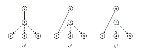
It is assumed that the communication graph for the $N+1$ agents is switched within a finite graph set $\widehat{\mathcal{G}}=\left{\mathcal{G}^{1}, \ldots, \mathcal{G}^{\kappa}\right}, \kappa>1$ and $\kappa \in \mathbb{N}$. Since the leader has no neighbors, the associated Laplacian matrix can be rewritten as
$$
\mathcal{L}^{\sigma(t)}=\left[\begin{array}{cc}
0 & \mathbf{0}{N}^{T} \ \mathbf{P} & \overline{\mathcal{L}}^{\sigma(t)} \end{array}\right] $$ where $\mathbf{P}=-\left[a{10}^{\sigma(t)}, \ldots, a_{N 0}^{\sigma(t)}\right]^{T}$, the piecewise constant function $\sigma(t):[0,+\infty) \mapsto$ ${1, \ldots, \kappa}$ represents the switching signal and satisfies the ADT condition (2.23).
Within the context of CNSs, each agent only communicates with its neighbors. Then the relative state information of other agents with respect to agent $i$ is given by
$$
\delta_{i}(t)=\sum_{j=0}^{N} a_{i j}^{\sigma(t)}\left(x_{j}(t)-x_{i}(t)\right), i=1, \ldots, N
$$
Note that $\delta_{i}(t)$ is a local information and thereby can be used for the controller design.
cs代写|复杂网络代写complex network代考|Main results for an autonomous leader case
In this subsection, the leader is assumed to be autonomous. That is, the dynamics of the leader are described by (3.27) with $f\left(x_{0}(t), t\right)=\mathbf{0}{m}$. To achieve consensus tracking, a distributed protocol is proposed as follows $$ u{i}(t)=c K \delta_{i}(t), \quad i=1, \ldots, N,
$$
where $\delta_{i}(t)$ is given in (3.29), $c>0$ and $K \in \mathbb{R}^{m \times n}$ are the control parameters to be designed later.
Let $e(t)=\left[e_{1}^{T}(t), \ldots, e_{N}^{T}(t)\right]^{T}$, where $e_{i}(t)=x_{i}(t)-x_{0}(t), i=1, \ldots, N$. Combining (3.26), (3.27) together with (3.30) yields
$$
\dot{e}(t)=\left[I_{N} \otimes A-c\left(\overline{\mathcal{L}}^{\sigma(t)} \otimes B K\right)\right] e(t) .
$$
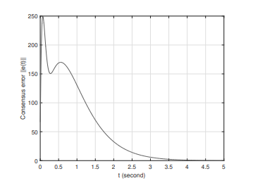
Obviously, the consensus tracking problem is solved if and only if $\lim _{t \rightarrow+\infty}|e(t)|=0$. That is, consensus tracking in the considered CNSs will be achieved if and only if the zero fixed point of switched systems (3.31) is globally attractive. Throughout the section, the derivatives of all signals at switching time instants should be considered as their right derivatives.
Before moving on, the following Assumption is made.
Assumption $3.2$ For each $i \in{1, \ldots, \kappa}$, the directed graph $\mathcal{G}^{i}$ contains a directed spanning tree rooted at node 0 (i.e., the leader).
Under Assumption 3.2, it can be obtained from Lemma $2.14$ that all the eigenvalues of $\overline{\mathcal{L}}^{i}$ have positive real parts, i.e., $\overline{\mathcal{L}}^{i}$ is anti-stable. Thus, the Lyapunov inequalities
$$
Q^{i} \overline{\mathcal{L}}^{i}+\left(\overline{\mathcal{L}}^{i}\right)^{T} Q^{i}>0
$$
are simultaneously feasible for some positive definite matrices $Q^{i}, i \in{1, \ldots, \kappa}$. Since the righ-hand side of $(3.32)$ is homogeneous for $Q^{i}$ for each $i \in{1, \ldots, \kappa}$, one gets that the matrix inequalities
$$
\bar{Q}^{i} \overline{\mathcal{L}}^{i}+\left(\overline{\mathcal{L}}^{i}\right)^{T} \bar{Q}^{i}>0, \bar{Q}^{i} \leq I_{N}, \text { and } \bar{Q}^{i}>0,
$$
are simultaneously feasible for some positive definite matrices $\bar{Q}^{i}$. To arrive at a less conservative estimation for the minimum allowable ADT for achieving consensus tracking, the following optimization algorithm is proposed.
cs代写|复杂网络代写complex network代考|Main results for a nonautonomous leader case
In this subsection, the leader is assumed to be a nonautonomous agent. To achieve consensus tracking, a distributed protocol is proposed as follows
$$
u_{i}(t)=d_{1} F \delta_{i}(t)+d_{2} \operatorname{sgn}\left(F \delta_{i}(t)\right), \quad i=1, \ldots, N,
$$
where $\delta_{i}(t)$ is given in (3.29), $d_{1}>0, d_{2}>0$, and $F \in \mathbb{R}^{m \times n}$ are the control parameters to be designed later, $\operatorname{sgn}(\cdot)$ denotes the element-wise sign function. For brevity, let $e(t)=\left[e_{1}^{T}(t), \ldots, e_{N}^{T}(t)\right]^{T}$ with $e_{i}(t)=x_{i}(t)-x_{0}(t)$. The tracking error system for the CNS (3.26) under protocol (3.59) with a nonautonomous leader (3.27) can be found to be
$$
\begin{aligned}
\dot{e}(t)=& {\left[I_{N} \otimes A-d_{1}\left(\overline{\mathcal{L}}^{\sigma(t)} \otimes B F\right)\right] e(t) } \
&-d_{2}\left(I_{N} \otimes B\right) \cdot \operatorname{sgn}\left(\left(\overline{\mathcal{L}}^{\sigma(t)} \otimes F\right) e(t)\right)-\left(\mathbf{1}{N} \otimes B\right) f\left(x{0}(t), t\right),
\end{aligned}
$$
where $\overline{\mathcal{L}}^{\sigma(t)}$ is given in (3.28). Note that the subsequent analysis is performed based on Assumption $3.2$ and the following assumption.
Assumption 3.5 There exists a positive scalar $d_{0}$ such that $\left|f\left(x_{0}(t), t\right)\right|_{\infty} \leq d_{0}$ for all $t \geq 0$.
It is worth noticing that Assumption $3.5$ provides an assurance preventing the actuators from blowing up physically. Note also that the explicit form of nonlinear function $f\left(x_{0}(t), t\right)$ is unknown to any follower. For notational brevity, let
$$
\bar{\kappa}{0}=\max {i, j \in{1, \ldots, \kappa}, i \neq j}\left{\bar{\chi}^{i} / \chi^{j}\right},
$$
where $\bar{\chi}^{i}=\lambda_{\max }\left(\left(\overline{\mathcal{L}}^{i}\right)^{T} \Phi^{i} \overline{\mathcal{L}}^{i}\right), \chi^{j}=\lambda_{\min }\left(\left(\overline{\mathcal{L}}^{i}\right)^{T} \Phi^{i} \overline{\mathcal{L}}^{i}\right)$, and matrices $\Phi^{i}, i \in{1, \ldots, \kappa}$, are determined in Algorithm $3.1$ by restricting $\bar{Q}^{i}$ and $\Omega^{i}$ to be positive definite and diagonal matrices. In this case, one knows that $\Phi^{i}, i \in{1, \ldots, \kappa}$, are all positive definite and diagonal matrices. Obviously, $\bar{\kappa}{0} \geq 1$. Furthermore, introduce $$ \chi{0}=\min {i \in{1, \ldots, \kappa}}\left{\lambda{\min }\left(\overline{\mathcal{L}}^{i}+\left(\Phi^{i}\right)^{-1}\left(\overline{\mathcal{L}}^{i}\right)^{T} \Phi^{i}\right)\right} .
$$
复杂网络代写
cs代写|复杂网络代写complex network代考|Model formulation
考虑一个由领导者和ñ追随者,其中领导者被标记为代理 0 ,追随者分别被标记为代理1,…,ñ. 动力学
代理人一世,一世=1,…,ñ, 由
X˙一世(吨)=一个X一世(吨)+乙在一世(吨)
在哪里X一世(吨)∈Rn和在一世(吨)∈R米分别是状态和控制输入,一个∈Rn×n和乙∈Rn×米分别是系统矩阵和输入矩阵。假使,假设(一个,乙)是稳定的。进一步假设领导者在这部分没有邻居,即领导者的动态不会受到任何追随者的影响。那么agent 0的动态描述为
X˙0(吨)=一个X0(吨)+乙F(X0(吨),吨),
在哪里X0(吨)∈Rn是领导者的状态,并且F(X0(吨),吨)∈R米是描述作用于领导者的外部控制输入的未知非线性函数。
假设通信图为ñ+1代理在有限图集中切换\widehat{\mathcal{G}}=\left{\mathcal{G}^{1}, \ldots, \mathcal{G}^{\kappa}\right}, \kappa>1\widehat{\mathcal{G}}=\left{\mathcal{G}^{1}, \ldots, \mathcal{G}^{\kappa}\right}, \kappa>1和ķ∈ñ. 由于领导者没有邻居,因此相关的拉普拉斯矩阵可以重写为
大号σ(吨)=[00ñ吨 磷大号¯σ(吨)]在哪里磷=−[一个10σ(吨),…,一个ñ0σ(吨)]吨, 分段常数函数σ(吨):[0,+∞)↦ 1,…,ķ表示开关信号,满足 ADT 条件(2.23)。
在 CNS 的上下文中,每个代理只与它的邻居通信。然后是其他代理相对于代理的相对状态信息一世是(谁)给的
d一世(吨)=∑j=0ñ一个一世jσ(吨)(Xj(吨)−X一世(吨)),一世=1,…,ñ
注意d一世(吨)是本地信息,因此可用于控制器设计。
cs代写|复杂网络代写complex network代考|Main results for an autonomous leader case
在本小节中,假设领导者是自治的。也就是说,领导者的动态由(3.27)描述F(X0(吨),吨)=0米. 为了实现共识跟踪,提出了一种分布式协议如下
在一世(吨)=Cķd一世(吨),一世=1,…,ñ,
在哪里d一世(吨)在 (3.29) 中给出,C>0和ķ∈R米×n是后面要设计的控制参数。
让和(吨)=[和1吨(吨),…,和ñ吨(吨)]吨, 在哪里和一世(吨)=X一世(吨)−X0(吨),一世=1,…,ñ. 将 (3.26)、(3.27) 和 (3.30) 结合起来,得到
和˙(吨)=[我ñ⊗一个−C(大号¯σ(吨)⊗乙ķ)]和(吨).
显然,共识跟踪问题得到解决当且仅当林吨→+∞|和(吨)|=0. 也就是说,当且仅当切换系统的零不动点 (3.31) 具有全局吸引力时,所考虑的 CNS 中的共识跟踪才能实现。在整个部分中,所有信号在切换时刻的导数都应被视为它们的右导数。
在继续之前,做出以下假设。
假设3.2对于每个一世∈1,…,ķ, 有向图G一世包含一个以节点 0 为根的有向生成树(即领导者)。
在假设 3.2 下,可以从引理得到2.14的所有特征值大号¯一世有正实部,即大号¯一世是反稳定的。因此,李雅普诺夫不等式
问一世大号¯一世+(大号¯一世)吨问一世>0
对一些正定矩阵同时可行问一世,一世∈1,…,ķ. 由于右手边(3.32)是同质的问一世对于每个一世∈1,…,ķ, 得到矩阵不等式
问¯一世大号¯一世+(大号¯一世)吨问¯一世>0,问¯一世≤我ñ, 和 问¯一世>0,
对一些正定矩阵同时可行问¯一世. 为了对实现共识跟踪的最小允许 ADT 进行不太保守的估计,提出了以下优化算法。
cs代写|复杂网络代写complex network代考|Main results for a nonautonomous leader case
在本小节中,领导者被假定为非自治代理。为了实现共识跟踪,提出了一种分布式协议如下
在一世(吨)=d1Fd一世(吨)+d2sgn(Fd一世(吨)),一世=1,…,ñ,
在哪里d一世(吨)在 (3.29) 中给出,d1>0,d2>0, 和F∈R米×n是后面要设计的控制参数,sgn(⋅)表示逐元素符号函数。为简洁起见,让和(吨)=[和1吨(吨),…,和ñ吨(吨)]吨和和一世(吨)=X一世(吨)−X0(吨). 可以发现具有非自治领导者(3.27)的协议(3.59)下的CNS(3.26)的跟踪误差系统是
和˙(吨)=[我ñ⊗一个−d1(大号¯σ(吨)⊗乙F)]和(吨) −d2(我ñ⊗乙)⋅sgn((大号¯σ(吨)⊗F)和(吨))−(1ñ⊗乙)F(X0(吨),吨),
在哪里大号¯σ(吨)在 (3.28) 中给出。注意后面的分析是基于Assumption进行的3.2和以下假设。
假设 3.5 存在一个正标量d0这样|F(X0(吨),吨)|∞≤d0对所有人吨≥0.
值得注意的是,假设3.5提供了防止执行器物理爆炸的保证。还要注意非线性函数的显式形式F(X0(吨),吨)任何追随者都不知道。为了符号简洁,令
$$
\bar{\kappa}{0}=\max {i, j \in{1, \ldots, \kappa}, i \neq j}\left{\bar{\chi}^ {i} / \chi ^{j}\right},
$$
其中 $\bar{\chi}^{i}=\lambda_{\max }\left(\left(\overline{\mathcal{L}} ^{i}\right)^{T} \Phi^{i} \overline{\mathcal{L}}^{i}\right), \chi ^{j}=\lambda_{\min }\left( \left(\overline{\mathcal{L}}^{i}\right)^{T} \Phi^{i} \overline{\mathcal{L}}^{i}\right),一个nd米一个吨r一世C和s\Phi^{i}, i \in{1, \ldots, \kappa},一个r和d和吨和r米一世n和d一世n一个lG○r一世吨H米3.1b是r和s吨r一世C吨一世nG\bar{Q}^{i}一个nd\欧米茄^{i}吨○b和p○s一世吨一世在和d和F一世n一世吨和一个ndd一世一个G○n一个l米一个吨r一世C和s.我n吨H一世sC一个s和,○n和ķn○在s吨H一个吨\Phi^{i}, i \in{1, \ldots, \kappa},一个r和一个llp○s一世吨一世在和d和F一世n一世吨和一个ndd一世一个G○n一个l米一个吨r一世C和s.○b在一世○在sl是,\bar {\kappa} {0} \geq 1.F在r吨H和r米○r和,一世n吨r○d在C和\chi{0}=\min {i \in{1, \ldots, \kappa}}\left{\lambda{\min }\left(\overline{\mathcal{L}}^{i}+\left (\Phi^{i}\right)^{-1}\left(\overline{\mathcal{L}}^{i}\right)^{T} \Phi^{i}\right)\right} .\chi{0}=\min {i \in{1, \ldots, \kappa}}\left{\lambda{\min }\left(\overline{\mathcal{L}}^{i}+\left (\Phi^{i}\right)^{-1}\left(\overline{\mathcal{L}}^{i}\right)^{T} \Phi^{i}\right)\right} .$

统计代写请认准statistics-lab™. statistics-lab™为您的留学生涯保驾护航。
金融工程代写
金融工程是使用数学技术来解决金融问题。金融工程使用计算机科学、统计学、经济学和应用数学领域的工具和知识来解决当前的金融问题,以及设计新的和创新的金融产品。
非参数统计代写
非参数统计指的是一种统计方法,其中不假设数据来自于由少数参数决定的规定模型;这种模型的例子包括正态分布模型和线性回归模型。
广义线性模型代考
广义线性模型(GLM)归属统计学领域,是一种应用灵活的线性回归模型。该模型允许因变量的偏差分布有除了正态分布之外的其它分布。
术语 广义线性模型(GLM)通常是指给定连续和/或分类预测因素的连续响应变量的常规线性回归模型。它包括多元线性回归,以及方差分析和方差分析(仅含固定效应)。
有限元方法代写
有限元方法(FEM)是一种流行的方法,用于数值解决工程和数学建模中出现的微分方程。典型的问题领域包括结构分析、传热、流体流动、质量运输和电磁势等传统领域。
有限元是一种通用的数值方法,用于解决两个或三个空间变量的偏微分方程(即一些边界值问题)。为了解决一个问题,有限元将一个大系统细分为更小、更简单的部分,称为有限元。这是通过在空间维度上的特定空间离散化来实现的,它是通过构建对象的网格来实现的:用于求解的数值域,它有有限数量的点。边界值问题的有限元方法表述最终导致一个代数方程组。该方法在域上对未知函数进行逼近。[1] 然后将模拟这些有限元的简单方程组合成一个更大的方程系统,以模拟整个问题。然后,有限元通过变化微积分使相关的误差函数最小化来逼近一个解决方案。
tatistics-lab作为专业的留学生服务机构,多年来已为美国、英国、加拿大、澳洲等留学热门地的学生提供专业的学术服务,包括但不限于Essay代写,Assignment代写,Dissertation代写,Report代写,小组作业代写,Proposal代写,Paper代写,Presentation代写,计算机作业代写,论文修改和润色,网课代做,exam代考等等。写作范围涵盖高中,本科,研究生等海外留学全阶段,辐射金融,经济学,会计学,审计学,管理学等全球99%专业科目。写作团队既有专业英语母语作者,也有海外名校硕博留学生,每位写作老师都拥有过硬的语言能力,专业的学科背景和学术写作经验。我们承诺100%原创,100%专业,100%准时,100%满意。
随机分析代写
随机微积分是数学的一个分支,对随机过程进行操作。它允许为随机过程的积分定义一个关于随机过程的一致的积分理论。这个领域是由日本数学家伊藤清在第二次世界大战期间创建并开始的。
时间序列分析代写
随机过程,是依赖于参数的一组随机变量的全体,参数通常是时间。 随机变量是随机现象的数量表现,其时间序列是一组按照时间发生先后顺序进行排列的数据点序列。通常一组时间序列的时间间隔为一恒定值(如1秒,5分钟,12小时,7天,1年),因此时间序列可以作为离散时间数据进行分析处理。研究时间序列数据的意义在于现实中,往往需要研究某个事物其随时间发展变化的规律。这就需要通过研究该事物过去发展的历史记录,以得到其自身发展的规律。
回归分析代写
多元回归分析渐进(Multiple Regression Analysis Asymptotics)属于计量经济学领域,主要是一种数学上的统计分析方法,可以分析复杂情况下各影响因素的数学关系,在自然科学、社会和经济学等多个领域内应用广泛。
MATLAB代写
MATLAB 是一种用于技术计算的高性能语言。它将计算、可视化和编程集成在一个易于使用的环境中,其中问题和解决方案以熟悉的数学符号表示。典型用途包括:数学和计算算法开发建模、仿真和原型制作数据分析、探索和可视化科学和工程图形应用程序开发,包括图形用户界面构建MATLAB 是一个交互式系统,其基本数据元素是一个不需要维度的数组。这使您可以解决许多技术计算问题,尤其是那些具有矩阵和向量公式的问题,而只需用 C 或 Fortran 等标量非交互式语言编写程序所需的时间的一小部分。MATLAB 名称代表矩阵实验室。MATLAB 最初的编写目的是提供对由 LINPACK 和 EISPACK 项目开发的矩阵软件的轻松访问,这两个项目共同代表了矩阵计算软件的最新技术。MATLAB 经过多年的发展,得到了许多用户的投入。在大学环境中,它是数学、工程和科学入门和高级课程的标准教学工具。在工业领域,MATLAB 是高效研究、开发和分析的首选工具。MATLAB 具有一系列称为工具箱的特定于应用程序的解决方案。对于大多数 MATLAB 用户来说非常重要,工具箱允许您学习和应用专业技术。工具箱是 MATLAB 函数(M 文件)的综合集合,可扩展 MATLAB 环境以解决特定类别的问题。可用工具箱的领域包括信号处理、控制系统、神经网络、模糊逻辑、小波、仿真等。