如果你也在 怎样代写电磁学electromagnetism这个学科遇到相关的难题,请随时右上角联系我们的24/7代写客服。
电磁学是电荷、磁矩和电磁场之间的物理互动。电磁场可以是静态的,缓慢变化的,或形成波。电磁波一般被称为光,遵守光学定律。
statistics-lab™ 为您的留学生涯保驾护航 在代写电磁学electromagnetism方面已经树立了自己的口碑, 保证靠谱, 高质且原创的统计Statistics代写服务。我们的专家在代写电磁学electromagnetism代写方面经验极为丰富,各种代写电磁学electromagnetism相关的作业也就用不着说。
我们提供的电磁学electromagnetism及其相关学科的代写,服务范围广, 其中包括但不限于:
- Statistical Inference 统计推断
- Statistical Computing 统计计算
- Advanced Probability Theory 高等概率论
- Advanced Mathematical Statistics 高等数理统计学
- (Generalized) Linear Models 广义线性模型
- Statistical Machine Learning 统计机器学习
- Longitudinal Data Analysis 纵向数据分析
- Foundations of Data Science 数据科学基础
物理代写|电磁学代写electromagnetism代考|Force Fields
The field forces act through space, producing an effect even when no physical contact between the objects occurs. As an example, we can mention the gravitational field. Michael Faraday developed a similar approach to electric forces. That is, an electric field exists in the region of space around any charged body, and when another charged body is inside this region of the electric field, an electric force acts on it.
Definition 1.2 The electric field $\mathbf{E}$ at a point in space is defined as the electric force $\mathbf{F}_e$ acting on a positive test charge $q_0$ placed at that point divided by the magnitude of the test charge:
$$
\mathbf{E}=\frac{\mathbf{F}_e}{q_0}
$$
The vector $\mathbf{E}$ has the SI units of newtons per coulomb (N/C). Figure $1.3$ illustrates the electric field $\mathbf{E}$ created by a positively charged sphere with total charge $Q$ at the positive test charge $q_0$. Here, we have assumed that the test charge $q_0$ is small enough that it does not disturb the charge distribution of the sphere responsible for the electric field.
Note that $\mathbf{E}$ is the field produced by some charge external to the test charge, and it is not the field produced by the test charge itself. Also, note that the existence of an electric field is a property of its source. For example, every electron comes with its electric field. An electric field exists at a point if a test charge at rest at that point experiences an electric force. The electric field direction is the direction of the force on a positive test charge placed in the field. Once we know the magnitude and direction of the electric field at some point, the electric force exerted on any charged particle (either positive or negative) placed at that point can be calculated. The electric field exists at some point space, including the free space, independent of the existence of another test charge at that point.
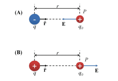
To determine the direction of electric field, consider a point charge $q$ located some distance $r$ from a test positive charge $q_0$ located at a point $P$, as shown in Fig. 1.4. Coulomb’s law defines the force exerted by $q$ on $q_0$ as
$$
\mathbf{F}_e=k_e \frac{q q_0}{r^2} \hat{\mathbf{r}}
$$
where $\hat{\mathbf{r}}$ represents the usual unit vector directed from $q$ toward $q_0$ (see Fig. 1.4). Electric field created by $q$ (positive or negative) is $$
\mathbf{E}=\frac{\mathbf{F}_e}{q_0}=k_e \frac{q}{r^2} \hat{\mathbf{r}}
$$
From Eq. (1.11), when $q<0$, then $\mathbf{E}$ is pointing opposite to vector $\hat{\mathbf{r}}$, and hence the electric field of a negative charge is pointing toward that charge, see Fig. 1.4a. On the other hand, when $q>0, \mathbf{E}$ and $\hat{\mathbf{r}}$ are parallel, and hence the electric field of a positive charge is pointing away from that charge, as shown in Fig. 1.4b.
物理代写|电磁学代写electromagnetism代考|Superposition Principle
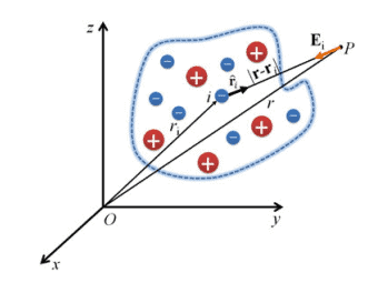
According to superposition principle, at any point $P$, the total electric field due to a set of discrete point charges, $q_1, q_2, \ldots, q_N$, positive and negative charges, is equal to the sum of the individual charge electric field vectors (see Fig. 1.5). Mathematically, we can write
$$
\mathbf{E}(\mathbf{r})=\sum_{i=1}^N \mathbf{E}i=\sum{i=1}^N k_e \frac{q_i}{\left|\mathbf{r}-\mathbf{r}_i\right|^2} \hat{\mathbf{r}}_i
$$
In Eq. (1.12), $\left|\mathbf{r}-\mathbf{r}_i\right|$ is the distance from $q_i$ to the point $P$ (the location of a test charge), where $\mathbf{r}$ is the position vector of the point $P$ with respect to some reference frame, as indicated in Fig. 1.5, and $\mathbf{r}_i$ is the position vector of the charge $i$ in that reference frame. Furthermore, $\hat{\mathbf{r}}_i$ is a unit vector directed from $q_i$ toward $P$.
Note that in Eq. (1.12) the dependence of $\mathbf{E}$ on only position vector of point $P$. r. assumes a static configuration of the charges in space. That is, for some other configuration distribution of charges in space, $\mathbf{E}$ at the same point $P$ may be different. Note that often for convenience, Eq.(1.12) is also written as $$
\mathbf{E}(\mathbf{r})=\sum_{i=1}^N k_e \frac{q_i\left(\mathbf{r}-\mathbf{r}_i\right)}{\left|\mathbf{r}-\mathbf{r}_i\right|^3}
$$
where
$$
\hat{\mathbf{r}}_i=\frac{\mathbf{r}-\mathbf{r}_i}{\left|\mathbf{r}-\mathbf{r}_i\right|}
$$
If the distances between charges in a set of charges are much smaller, compare with the distance of the set from a point where the electric field is to be calculated, then charge distribution is continuous.
To calculate the net electric field created by a continuous charge distribution in some volume $V$, we follow these steps. First, we divide the charge distribution into macroscopically small elements with small charge $\Delta q_i$, as shown in Fig. 1.6a. $\Delta q_i=\rho_i \Delta V$, where $\rho_i$ is seen from a microscopic viewpoint as a uniform charge density within the volume element $i$, which represents one of the possible configurations of microscopic description. It is important to note that with “macroscopically small” we should understand a small volume in space with a characteristic microscopic configuration of the charges inside it that can, on average, macroscopically be represented as a point-like charge, $\Delta q_i$. Then, we calculate the electric field due to one of these macroscopically point charges, $\Delta q_i$, at some point $P$ at distance $\left|\mathbf{r}-\mathbf{r}_i\right|$ from the charge element, $\Delta q_i$, as
$$
\Delta \mathbf{E}\left(\mathbf{r}, \mathbf{r}_i\right)=k_e \frac{\Delta q_i}{\left|\mathbf{r}-\mathbf{r}_i\right|^2} \hat{\mathbf{r}}_i
$$
where $\hat{\mathbf{r}}_i$ is a unit vector directed from the charge element $\Delta q_i$ toward $P$. Here, $\mathbf{r}$ is position vector of point $P$ in some reference frame, and $\mathbf{r}_i$ is the position vector of the macroscopically point charge $\Delta q_i$.
电磁学代考
物理代写|电磁学代写electromagnetism代考|Force Fields
场力通过空间作用,即使在物体之间没有发生物理接触时也会产生效果。例如,我们可以提到引力场。 迈克尔法拉第开发了一种类似的电力方法。也就是说,任何带电体周围的空间区域都存在电场,当另一 个带电体位于该电场区域内时,就会对其作用电力。
定义 $1.2$ 电场 $\mathbf{E}$ 在空间中的一点被定义为电力 $\mathbf{F}_e$ 作用于正测试电荷 $q_0$ 放置在该点除以测试电荷的大小:
$$
\mathbf{E}=\frac{\mathbf{F}_e}{q_0}
$$
载体 $\mathbf{E}$ 具有牛顿每库仑 (N/C) 的 SI 单位。数字1.3说明电场 $\mathbf{E}$ 由带总电荷的带正电的球体产生 $Q$ 在积极的 测试电荷 $q_0$. 在这里,我们假设测试充电 $q_0$ 足够小,不会干扰负责电场的球体的电荷分布。
注意 $\mathbf{E}$ 是由测试电荷外部的一些电荷产生的场,而不是由测试电荷本身产生的场。另请注意,电场的存在 是其来源的一个属性。例如,每个电子都带有电场。如果静止的测试电荷在该点受到电力,则该点存在 电场。电场方向是放置在场中的正测试电荷所受力的方向。一旦我们知道某一点电场的大小和方向,就 可以计算出施加在该点的任何带电粒子(正或负)上的电力。电场存在于空间的某一点,包括自由空 间,与该点是否存在另一个测试电荷无关。
要确定电场的方向,请考虑点电荷 $q$ 位于一定距离 $r$ 来自测试正电荷 $q_0$ 位于一个点 $P$ ,如图1.4所示。库仑 定律定义了施加的力 $q$ 在 $q_0$ 作为
$$
\mathbf{F}_e=k_e \frac{q q_0}{r^2} \hat{\mathbf{r}}
$$
在哪里 $\hat{\mathbf{r}}$ 表示通常的单位向量 $q$ 朝向 $q_0$ (见图 1.4)。产生的电场 $q$ (正面或负面) 是
$$
\mathbf{E}=\frac{\mathbf{F}_e}{q_0}=k_e \frac{q}{r^2} \hat{\mathbf{r}}
$$
从等式。(1.11),当 $q<0$ ,然后 $\mathbf{E}$ 指向向量的对面 $\hat{\mathbf{r}}$ ,因此负电荷的电场指向该电荷,见图 1.4a。另一 方面,当 $q>0, \mathbf{E}$ 和 $\hat{\mathbf{r}}$ 是平行的,因此正电荷的电场指向远离该电荷的方向,如图 1.4b 所示。
物理代写|电磁学代写electromagnetism代考|Superposition Principle
根据㢶加原理,任意一点 $P$ ,由于一组离散点电荷引起的总电场, $q_1, q_2, \ldots, q_N$ ,正电荷和负电荷,等 于各个电荷电场矢量的总和 (见图 1.5)。在数学上,我们可以写
$$
\mathbf{E}(\mathbf{r})=\sum_{i=1}^N \mathbf{E} i=\sum i=1^N k_e \frac{q_i}{\left|\mathbf{r}-\mathbf{r}i\right|^2} \hat{\mathbf{r}}_i $$ 在等式中。(1.12), $\left|\mathbf{r}-\mathbf{r}_i\right|$ 是距离 $q_i$ 直截了当 $P$ (测试电荷的位置),其中 $\mathbf{r}$ 是点的位置向量 $P$ 关于一些 参考系,如图 1.5 所示,以及 $\mathbf{r}_i$ 是电荷的位置向量 $i$ 在那个参考系中。此外, $\hat{\mathbf{r}}_i$ 是指向的单位向量 $q_i$ 朝向 $P$. 请注意,在等式中。(1.12) 的依赖 $\mathbf{E}$ 仅在点的位置向量上 $P$. 河 假定空间中电荷的静态配置。也就是说, 对于空间中电荷的一些其他配置分布, $\mathbf{E}$ 在同一时间 $P$ 可能不同。请注意,通常为方便起见,Eq.(1.12) 也写为 $$ \mathbf{E}(\mathbf{r})=\sum{i=1}^N k_e \frac{q_i\left(\mathbf{r}-\mathbf{r}_i\right)}{\left|\mathbf{r}-\mathbf{r}_i\right|^3}
$$
在哪里
$$
\hat{\mathbf{r}}_i=\frac{\mathbf{r}-\mathbf{r}_i}{\left|\mathbf{r}-\mathbf{r}_i\right|}
$$
如果一组电荷中的电荷之间的距离远小于该组到要计算电场的点的距离,则电荷分布是连续的。
计算由某个体积中的连续电荷分布产生的净电场 $V$ ,我们按照这些步骤。首先,我们将电荷分布划分为具 有小电荷的宏观小元素 $\Delta q_i$ ,如图 1.6a 所示。 $\Delta q_i=\rho_i \Delta V$ , 在哪里 $\rho_i$ 从微观角度看是体积元内均匀 的电荷密度 $i$ ,它代表了微观描述的一种可能配置。重要的是要注意,对于“宏观上小”,我们应该理解空 间中的小体积,其内部电荷具有特征性的微观结构,平均而言,可以宏观地表示为点状电荷, $\Delta q_i$. 然 后,我们计算由这些宏观点电荷之一引起的电场, $\Delta q_i$ , 在某一点 $P$ 在远处 $\left|\mathbf{r}-\mathbf{r}_i\right|$ 从电荷元素, $\Delta q_i$ ,作为
$$
\Delta \mathbf{E}\left(\mathbf{r}, \mathbf{r}_i\right)=k_e \frac{\Delta q_i}{\left|\mathbf{r}-\mathbf{r}_i\right|^2} \hat{\mathbf{r}}_i
$$
在哪里 $\hat{\mathbf{r}}_i$ 是从电荷元素指向的单位向量 $\Delta q_i$ 朝向 $P$. 这里, $\mathbf{r}$ 是点的位置向量 $P$ 在一些参考系中,和 $\mathbf{r}_i$ 是 宏观点电荷的位置矢量 $\Delta q_i$.

统计代写请认准statistics-lab™. statistics-lab™为您的留学生涯保驾护航。
金融工程代写
金融工程是使用数学技术来解决金融问题。金融工程使用计算机科学、统计学、经济学和应用数学领域的工具和知识来解决当前的金融问题,以及设计新的和创新的金融产品。
非参数统计代写
非参数统计指的是一种统计方法,其中不假设数据来自于由少数参数决定的规定模型;这种模型的例子包括正态分布模型和线性回归模型。
广义线性模型代考
广义线性模型(GLM)归属统计学领域,是一种应用灵活的线性回归模型。该模型允许因变量的偏差分布有除了正态分布之外的其它分布。
术语 广义线性模型(GLM)通常是指给定连续和/或分类预测因素的连续响应变量的常规线性回归模型。它包括多元线性回归,以及方差分析和方差分析(仅含固定效应)。
有限元方法代写
有限元方法(FEM)是一种流行的方法,用于数值解决工程和数学建模中出现的微分方程。典型的问题领域包括结构分析、传热、流体流动、质量运输和电磁势等传统领域。
有限元是一种通用的数值方法,用于解决两个或三个空间变量的偏微分方程(即一些边界值问题)。为了解决一个问题,有限元将一个大系统细分为更小、更简单的部分,称为有限元。这是通过在空间维度上的特定空间离散化来实现的,它是通过构建对象的网格来实现的:用于求解的数值域,它有有限数量的点。边界值问题的有限元方法表述最终导致一个代数方程组。该方法在域上对未知函数进行逼近。[1] 然后将模拟这些有限元的简单方程组合成一个更大的方程系统,以模拟整个问题。然后,有限元通过变化微积分使相关的误差函数最小化来逼近一个解决方案。
tatistics-lab作为专业的留学生服务机构,多年来已为美国、英国、加拿大、澳洲等留学热门地的学生提供专业的学术服务,包括但不限于Essay代写,Assignment代写,Dissertation代写,Report代写,小组作业代写,Proposal代写,Paper代写,Presentation代写,计算机作业代写,论文修改和润色,网课代做,exam代考等等。写作范围涵盖高中,本科,研究生等海外留学全阶段,辐射金融,经济学,会计学,审计学,管理学等全球99%专业科目。写作团队既有专业英语母语作者,也有海外名校硕博留学生,每位写作老师都拥有过硬的语言能力,专业的学科背景和学术写作经验。我们承诺100%原创,100%专业,100%准时,100%满意。
随机分析代写
随机微积分是数学的一个分支,对随机过程进行操作。它允许为随机过程的积分定义一个关于随机过程的一致的积分理论。这个领域是由日本数学家伊藤清在第二次世界大战期间创建并开始的。
时间序列分析代写
随机过程,是依赖于参数的一组随机变量的全体,参数通常是时间。 随机变量是随机现象的数量表现,其时间序列是一组按照时间发生先后顺序进行排列的数据点序列。通常一组时间序列的时间间隔为一恒定值(如1秒,5分钟,12小时,7天,1年),因此时间序列可以作为离散时间数据进行分析处理。研究时间序列数据的意义在于现实中,往往需要研究某个事物其随时间发展变化的规律。这就需要通过研究该事物过去发展的历史记录,以得到其自身发展的规律。
回归分析代写
多元回归分析渐进(Multiple Regression Analysis Asymptotics)属于计量经济学领域,主要是一种数学上的统计分析方法,可以分析复杂情况下各影响因素的数学关系,在自然科学、社会和经济学等多个领域内应用广泛。
MATLAB代写
MATLAB 是一种用于技术计算的高性能语言。它将计算、可视化和编程集成在一个易于使用的环境中,其中问题和解决方案以熟悉的数学符号表示。典型用途包括:数学和计算算法开发建模、仿真和原型制作数据分析、探索和可视化科学和工程图形应用程序开发,包括图形用户界面构建MATLAB 是一个交互式系统,其基本数据元素是一个不需要维度的数组。这使您可以解决许多技术计算问题,尤其是那些具有矩阵和向量公式的问题,而只需用 C 或 Fortran 等标量非交互式语言编写程序所需的时间的一小部分。MATLAB 名称代表矩阵实验室。MATLAB 最初的编写目的是提供对由 LINPACK 和 EISPACK 项目开发的矩阵软件的轻松访问,这两个项目共同代表了矩阵计算软件的最新技术。MATLAB 经过多年的发展,得到了许多用户的投入。在大学环境中,它是数学、工程和科学入门和高级课程的标准教学工具。在工业领域,MATLAB 是高效研究、开发和分析的首选工具。MATLAB 具有一系列称为工具箱的特定于应用程序的解决方案。对于大多数 MATLAB 用户来说非常重要,工具箱允许您学习和应用专业技术。工具箱是 MATLAB 函数(M 文件)的综合集合,可扩展 MATLAB 环境以解决特定类别的问题。可用工具箱的领域包括信号处理、控制系统、神经网络、模糊逻辑、小波、仿真等。