如果你也在 怎样代写电动力学electrodynamics这个学科遇到相关的难题,请随时右上角联系我们的24/7代写客服。
电动力学是物理学的一个分支,处理快速变化的电场和磁场。
statistics-lab™ 为您的留学生涯保驾护航 在代写电动力学electrodynamics方面已经树立了自己的口碑, 保证靠谱, 高质且原创的统计Statistics代写服务。我们的专家在代写电动力学electrodynamics代写方面经验极为丰富,各种代写电动力学electrodynamics相关的作业也就用不着说。
我们提供的电动力学electrodynamics及其相关学科的代写,服务范围广, 其中包括但不限于:
- Statistical Inference 统计推断
- Statistical Computing 统计计算
- Advanced Probability Theory 高等概率论
- Advanced Mathematical Statistics 高等数理统计学
- (Generalized) Linear Models 广义线性模型
- Statistical Machine Learning 统计机器学习
- Longitudinal Data Analysis 纵向数据分析
- Foundations of Data Science 数据科学基础
物理代写|电动力学代写electromagnetism代考|ELECTRIC POTENTIAL
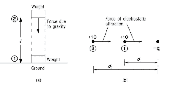
We often come across the term potential when applied to the potential energy of a body or the potential difference between two points in a circuit. In the former case, the potential energy of a body is related to its height above a certain reference level. Thus, a body gains potential energy when we raise it to a higher level. This gain in energy is equal to the work done against an attractive force, gravity in this example. Figure 2.6a shows this situation.
As Figure 2.6a shows, the body is placed in an attractive, gravitational force field. So, if we raise the body through a certain distance, we have to do work against the gravitational field. The difference in potential energy between positions 1 and 2 is equal to the work done in moving the body from 1 to 2 , a distance of $l$ metres. This work done is given by
$$
F \times l=m \times 9.81 \times l
$$
where $m$ is the mass of the body $(\mathrm{kg})$ and $9.81$ is the acceleration due to gravity $\left(\mathrm{m} \mathrm{s}^{-2}\right.$ ). (Although the effects of gravity vary according to the inverse square law, the difference in gravitational force between positions 1 and 2 is small. This is because the Earth is so large. Thus, we can take the gravitational field to be linear in form, and so this equation holds true.)
In an electrostatic field, we have an electrostatic force field instead of a gravitational force field. However, the idea of potential energy is the same. Let us consider the situation in Figure 2.6b. We have a positive test charge of $1 \mathrm{C}$ at a distance $\mathrm{d}_1$ from the fixed negative charge, $-q_1$. This test charge will experience an attractive force whose magnitude we can find from Coulomb’s law. Now, if we move the test charge from position 1 to position 2, we have to do work against the field. If the distance between positions 1 and 2 is reasonably large, the strength of the force field decreases as we move away from the fixed charge. Thus, we say that we have a non-linear field.
As the field decreases when we move away from the fixed charge, let us move the test charge a very small distance, $\mathrm{d} r$. The electric field strength will hardly alter as we move along this small distance. So, the work done against the field in moving the test charge a small distance $\mathrm{d} r$ will be given by
$$
\begin{aligned}
\text { work done } &=\text { force } \times \text { distance } \
&=-F \times \mathrm{d} r \
&=-1 \times E \times \mathrm{d} r
\end{aligned}
$$
物理代写|电动力学代写electromagnetism代考|EQUIPOTENTIAL LINES
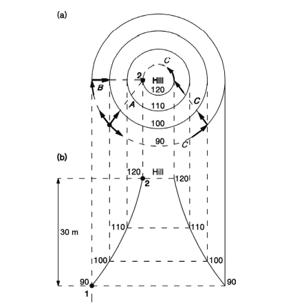
Let us consider the three paths $\mathrm{A}, \mathrm{B}$ and $\mathrm{C}$ shown in Figure $2.7 \mathrm{a}$. All of these paths link points 1 and 2, but only path A does so directly. Now, let us take the circular lines in Figure 2.7a as the contours on a hill. In moving from position 1 to position 2 by way of path $\mathrm{A}$, we clearly do work against gravity. The work done is equal to the gain in potential energy which, in turn, is equal to the gravitational force times the change in vertical height. (This is shown in Figure 2.7b.)
Now let us take path B. We initially walk left from position 1, around the contour line, to a point directly below position 2. As we have moved around a contour line, we have not gained any height, and so the potential energy remains the same, i.e., we have not done any work against gravity. We now have to walk uphill to position 2 . In doing so we do work against gravity equal to the gain in potential energy. This gain in potential energy is clearly the same as with path $\mathrm{A}$. (Although we have to do more physical work in travelling along path $\mathrm{B}$, the change in potential energy is the same.) If we use path $\mathrm{C}$, the same argument holds true. So, we can say that the work done against gravity is independent of the path we take.
Let us now turn our attention to the electrostatic field in Figure 2.8. As with the contour map, we have three different paths. As we have just seen, we do no work against the field when we move in a circular direction. We only do work when we move in a radial direction. Thus, the potential difference between points 1 and 2 is independent of the exact path we take. This implies that we do no work against the field when we move around the plot in a circular direction. Thus, the circular ‘contours’ in Figure $2.8$ are lines of equal potential or equipotential lines.
We should be careful when using the term equipotential lines. This is because we are considering a point charge, and so the equipotential surfaces are actually spheres with the charge at their centre. As we are not yet able to draw in a three-dimensional holographic world, we have to make do with two-dimensional diagrams drawn on pieces of paper!
电动力学代考
物理代写|电动力学代写electromagnetism代考|ELECTRIC POTENTIAL
当应用于身体的势能或电路中两点之间的电位差时,我们经常遇到术语电位。在前一种情况下,物体的 势能与其高于某个参考水平的高度有关。因此,当我们将身体提升到更高的水平时,它就会获得势能。 这种能量增益等于抵抗吸引力所做的功,在这个例子中是重力。图 2.6a 显示了这种情况。
如图 2.6a 所示,物体被放置在一个有吸引力的引力场中。所以,如果我们将身体抬高一段距离,我们 就必须对抗引力场。位置 1 和 2 之间的势能差等于将物体从 1 移动到 2 所做的功,距离为 $l$ 米。完成的 这项工作由
$$
F \times l=m \times 9.81 \times l
$$
在哪里 $m$ 是身体的质量 $(\mathrm{kg})$ 和 $9.81$ 是重力加速度 $\left(\mathrm{ms}^{-2}\right)$ 。(虽然重力的影响根据平方反比定律而变 化,但位置1和2之间的引力差异很小。这是因为地球太大了。因此,我们可以将引力场取为线性形 式,所以这个等式成立。)
在静电场中,我们有一个静电力场而不是重力场。然而,势能的概念是一样的。让我们考虑图 2.6b 中 的情况。我们有一个阳性测试电荷 $1 \mathrm{C}$ 在远处 $\mathrm{d}_1$ 从固定的负电荷, $-q_1$. 这个测试电荷将经历一个吸引 力,我们可以从库仑定律中找到它的大小。现在,如果我们将测试装药从位置 1 移到位置 2,我们必须 对场进行工作。如果位置 1 和 2 之间的距离相当大,则力场的强度会随着我们远离固定电荷而减小。 因此,我们说我们有一个非线性场。
当我们远离固定电荷时场减小,让我们将测试电荷移动一个很小的距离, $\mathrm{d} r$. 当我们沿着这个小距离移 动时,电场强度几平不会改变。因此,在将测试电荷移动一小段距离时对场所做的工作 $\mathrm{d} r$ 将由
$$
\text { work done }=\text { force } \times \text { distance } \quad=-F \times \mathrm{d} r=-1 \times E \times \mathrm{d} r
$$
物理代写|电动力学代写electromagnetism代考|EQUIPOTENTIAL LINES
让我们考虑三个路径一个,乙和C如图2.7一个. 所有这些路径都链接点 1 和 2,但只有路径 A 直接链接。现在,让我们将图 2.7a 中的圆形线作为山上的等高线。通过路径从位置 1 移动到位置 2一个,我们显然确实在对抗重力。所做的功等于势能的增益,而势能的增益又等于重力乘以垂直高度的变化。(如图 2.7b 所示。)
现在让我们走路径 B。我们最初从位置 1 沿等高线向左走,到位置 2 正下方的一点。由于我们绕着等高线移动,我们没有获得任何高度,因此势能保持不变同样,即我们没有做任何对抗重力的工作。我们现在必须上山到位置 2 。在这样做的过程中,我们确实对抗重力,等于增加了势能。势能的这种增益显然与路径相同一个. (虽然我们要在路上做更多的体力劳动乙,势能的变化是相同的。)如果我们使用路径C,同样的论点成立。因此,我们可以说对抗重力所做的功与我们所走的路径无关。
现在让我们把注意力转向图 2.8 中的静电场。与等高线图一样,我们有三种不同的路径。正如我们刚刚看到的,当我们沿圆周方向移动时,我们不会对场做任何工作。我们只有在径向移动时才工作。因此,点 1 和 2 之间的电位差与我们采用的确切路径无关。这意味着当我们在地块上沿圆形方向移动时,我们不会对场进行任何操作。因此,图中的圆形“轮廓”2.8是等势线或等势线。
我们在使用等势线这个词时要小心。这是因为我们正在考虑点电荷,因此等势面实际上是球体,电荷位于其中心。由于我们还不能在三维全息世界中绘画,所以我们不得不在纸上绘制二维图!

统计代写请认准statistics-lab™. statistics-lab™为您的留学生涯保驾护航。
金融工程代写
金融工程是使用数学技术来解决金融问题。金融工程使用计算机科学、统计学、经济学和应用数学领域的工具和知识来解决当前的金融问题,以及设计新的和创新的金融产品。
非参数统计代写
非参数统计指的是一种统计方法,其中不假设数据来自于由少数参数决定的规定模型;这种模型的例子包括正态分布模型和线性回归模型。
广义线性模型代考
广义线性模型(GLM)归属统计学领域,是一种应用灵活的线性回归模型。该模型允许因变量的偏差分布有除了正态分布之外的其它分布。
术语 广义线性模型(GLM)通常是指给定连续和/或分类预测因素的连续响应变量的常规线性回归模型。它包括多元线性回归,以及方差分析和方差分析(仅含固定效应)。
有限元方法代写
有限元方法(FEM)是一种流行的方法,用于数值解决工程和数学建模中出现的微分方程。典型的问题领域包括结构分析、传热、流体流动、质量运输和电磁势等传统领域。
有限元是一种通用的数值方法,用于解决两个或三个空间变量的偏微分方程(即一些边界值问题)。为了解决一个问题,有限元将一个大系统细分为更小、更简单的部分,称为有限元。这是通过在空间维度上的特定空间离散化来实现的,它是通过构建对象的网格来实现的:用于求解的数值域,它有有限数量的点。边界值问题的有限元方法表述最终导致一个代数方程组。该方法在域上对未知函数进行逼近。[1] 然后将模拟这些有限元的简单方程组合成一个更大的方程系统,以模拟整个问题。然后,有限元通过变化微积分使相关的误差函数最小化来逼近一个解决方案。
tatistics-lab作为专业的留学生服务机构,多年来已为美国、英国、加拿大、澳洲等留学热门地的学生提供专业的学术服务,包括但不限于Essay代写,Assignment代写,Dissertation代写,Report代写,小组作业代写,Proposal代写,Paper代写,Presentation代写,计算机作业代写,论文修改和润色,网课代做,exam代考等等。写作范围涵盖高中,本科,研究生等海外留学全阶段,辐射金融,经济学,会计学,审计学,管理学等全球99%专业科目。写作团队既有专业英语母语作者,也有海外名校硕博留学生,每位写作老师都拥有过硬的语言能力,专业的学科背景和学术写作经验。我们承诺100%原创,100%专业,100%准时,100%满意。
随机分析代写
随机微积分是数学的一个分支,对随机过程进行操作。它允许为随机过程的积分定义一个关于随机过程的一致的积分理论。这个领域是由日本数学家伊藤清在第二次世界大战期间创建并开始的。
时间序列分析代写
随机过程,是依赖于参数的一组随机变量的全体,参数通常是时间。 随机变量是随机现象的数量表现,其时间序列是一组按照时间发生先后顺序进行排列的数据点序列。通常一组时间序列的时间间隔为一恒定值(如1秒,5分钟,12小时,7天,1年),因此时间序列可以作为离散时间数据进行分析处理。研究时间序列数据的意义在于现实中,往往需要研究某个事物其随时间发展变化的规律。这就需要通过研究该事物过去发展的历史记录,以得到其自身发展的规律。
回归分析代写
多元回归分析渐进(Multiple Regression Analysis Asymptotics)属于计量经济学领域,主要是一种数学上的统计分析方法,可以分析复杂情况下各影响因素的数学关系,在自然科学、社会和经济学等多个领域内应用广泛。
MATLAB代写
MATLAB 是一种用于技术计算的高性能语言。它将计算、可视化和编程集成在一个易于使用的环境中,其中问题和解决方案以熟悉的数学符号表示。典型用途包括:数学和计算算法开发建模、仿真和原型制作数据分析、探索和可视化科学和工程图形应用程序开发,包括图形用户界面构建MATLAB 是一个交互式系统,其基本数据元素是一个不需要维度的数组。这使您可以解决许多技术计算问题,尤其是那些具有矩阵和向量公式的问题,而只需用 C 或 Fortran 等标量非交互式语言编写程序所需的时间的一小部分。MATLAB 名称代表矩阵实验室。MATLAB 最初的编写目的是提供对由 LINPACK 和 EISPACK 项目开发的矩阵软件的轻松访问,这两个项目共同代表了矩阵计算软件的最新技术。MATLAB 经过多年的发展,得到了许多用户的投入。在大学环境中,它是数学、工程和科学入门和高级课程的标准教学工具。在工业领域,MATLAB 是高效研究、开发和分析的首选工具。MATLAB 具有一系列称为工具箱的特定于应用程序的解决方案。对于大多数 MATLAB 用户来说非常重要,工具箱允许您学习和应用专业技术。工具箱是 MATLAB 函数(M 文件)的综合集合,可扩展 MATLAB 环境以解决特定类别的问题。可用工具箱的领域包括信号处理、控制系统、神经网络、模糊逻辑、小波、仿真等。