如果你也在 怎样代写金融实证Financial Empirical这个学科遇到相关的难题,请随时右上角联系我们的24/7代写客服。
金融实证是一个研究领域,涵盖了金融经济学的实证工作、金融计量经济学和具有明显实证意义的理论驱动研究。我们的研究人员调查的问题主要集中在资本市场、金融机构和企业融资等广泛领域。
statistics-lab™ 为您的留学生涯保驾护航 在代写金融实证Financial Empirical方面已经树立了自己的口碑, 保证靠谱, 高质且原创的统计Statistics代写服务。我们的专家在代写金融实证Financial Empirical股权市场金融实证Financial Empirical相关的作业也就用不着说。
我们提供的金融实证Financial Empirical及其相关学科的代写,服务范围广, 其中包括但不限于:
- Statistical Inference 统计推断
- Statistical Computing 统计计算
- Advanced Probability Theory 高等楖率论
- Advanced Mathematical Statistics 高等数理统计学
- (Generalized) Linear Models 广义线性模型
- Statistical Machine Learning 统计机器学习
- Longitudinal Data Analysis 纵向数据分析
- Foundations of Data Science 数据科学基础
金融代写|金融实证代写Financial Empirical 代考|Base Model
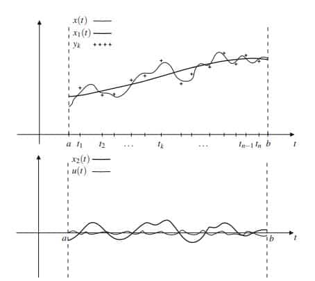
Based on the above discussion a time series $x(t)$ with possibly continuous time index $t$ in an interval $[a, b]$ will be analysed and additively decomposed in the unobservable important and interpretable components trend (and economic cycle) $x_1(t)$ and season (and calendar) $x_2(t)$. The rest $u(t)$ contains the unimportant, irregular unobservable parts, maybe containing additive outliers.
An “ideal” trend $\tilde{x}1(t)$ is represented by a polynomial of given degree $p-1$ and an “ideal” season $\tilde{x}_2(t)$ is represented by a linear combination of trigonometric functions of chosen frequencies (found by exploration) $\omega_j=2 \pi / S_j$ with $S_j=$ $S / n_j$ and $n_j \in \mathbb{N}$ for $j=1, \ldots, q$. Here $S$ is the known base period and $S_j$ leads to selected harmonics, which can be defined by Fourier analysis. Therefore holds $$ \tilde{x}_1(t)=\sum{j=0}^{p-1} a_j t^j \quad \text { and } \quad \tilde{x}2(t)=\sum{j=1}^q\left(b_{1 j} \cos \omega_j t+b_{2 j} \sin \omega_j t\right), \quad t \in[a, b] .
$$
In applications the components $x_1(t)$ and $x_2(t)$ won’t exist in ideal representation. They will be additively superimposed by random disturbances $u_1(t)$ and $u_2(t)$. Only at some points in time $t_1, \ldots, t_n$ in the time interval $[a, b]$ the sum $x(t)$ of components is observable, maybe flawed by further additive errors $\varepsilon_1, \ldots, \varepsilon_n$. The respective measurements are called $y_1, \ldots, y_n$.
Now we have following base model
$x_1(t)=\ddot{x}_1(t)+u_1(t)$
$x_2(t)=\tilde{x}_2(t)+u_2(t) \quad t \in[a, b] \quad$ state equation
$y_k=x_1\left(t_k\right)+x_2\left(t_k\right)+\varepsilon_k, \quad k=1, \ldots, n \quad$ observation equation,
cf. Fig. 1 .
金融代写|金融实证代写Financial Empirical 代考|Construction of the Estimation Principle
For evaluation of smoothness (in contrast to flexibility) the following smoothness measures are constructed (actually these are roughness measures).
By differentiation $\mathrm{D}=\frac{\mathrm{d}}{\mathrm{d} t}$ the degree of a polynomial is reduced by 1 . Therefore for a trend $x_1(t)$ as polynomial of degree $p-1$ always holds $\mathrm{D}^p x_1(t)=0$. On the
other hand, every function $x_1(t)$ with this feature is a polynomial of degree $p-1$. Therefore
$$
Q_1\left(x_1\right)=\int_a^b\left|\mathrm{D}^p x_1(t)\right|^2 \mathrm{~d} t \quad \text { measure of smoothness of trend }
$$
is a measure of the smoothness of an appropriately chosen function $x_1$.
For any sufficiently often differentiable and quadratically integrable function $x_1$ in interval $[a, b] Q_1\left(x_1\right)$ is zero iff $x_1$ is there a polynomial of degree $p-1$, i.e. $x_1(t)=\sum_{j=0}^{p-1} a_j t^j$, a smoothest (ideal) trend. The larger the value of $Q_1$ for a function $x_1$ in $[a, b]$ the larger is the deviation of $x_1$ from a (ideal) trend polynomial of degree $p-1$.
Two times differentiation of the functions $\cos \omega_j t$ and $\sin \omega_j t$ gives $-\omega_j^2 \cos \omega_j t$ and $-\omega_j^2 \sin \omega_j t$ such that $\prod_{j=1}^q\left(\mathrm{D}^2+\omega_j^2 \mathrm{I}\right)$ (I: identity) nullifies any linear combination $x_2(t)$ of all functions $\cos \omega_j t$ and $\sin \omega_j t, j=1, \ldots, q$. That is because the following
$$
\begin{aligned}
&\left(\mathrm{D}^2+\omega_j^2 \mathrm{I}\right)\left(b_{1 k} \cos \omega_k t+b_{2 k} \sin \omega_k t\right)= \
&=b_{1 k}\left(\omega_j^2-\omega_k^2\right) \cos \omega_k t+b_{2 k}\left(\omega_j^2-\omega_k^2\right) \sin \omega_k t \quad \text { for } \quad j, k=1, \ldots, q,
\end{aligned}
$$
nullifies for the case $j=k$ the respective oscillation. This also proves the exchangeability of the operators $\mathrm{D}^2+\omega_j^2 \mathrm{I}, j=1, \ldots, q$.
If inversely $\prod_{j=1}^q\left(\mathrm{D}^2+\omega_j^2 \mathrm{I}\right) x_2(t)=0$ holds, the function $x_2(t)$ is a linear combination of the trigonometric functions under investigation. Consequently
$Q_2\left(x_2\right)=\int_a^b\left|\prod_{j=1}^q\left(\mathrm{D}^2+\omega_j^2 \mathrm{I}\right) x_2(t)\right|^2 \mathrm{~d} t \quad$ measure of seasonal smoothness is a measure for seasonal smoothness of the chosen function $x_2$.
金融实证代考
金融代写|金融实证代写Financial Empirical 代考|Base Model
基于上述讨论,时间序列 $x(t)$ 具有可能连续的时间索引 $t$ 在一个区间 $[a, b]$ 将在不可观察的重要和可解释的成分趋 势 (和经济周期) 中进行分析和加法分解 $x_1(t)$ 和季节 (和日历) $x_2(t)$. 其余的部分 $u(t)$ 包含不重要的、不规则 的不可观察部分,可能包含附加异常值。
“理想”的趋势 $\tilde{x} 1(t)$ 由给定次数的多项式表示 $p-1$ 和一个“理想”的李节 $\tilde{x}2(t)$ 由选定频率的三角函数的线性组合表 示 (通过探索发现) $\omega_j=2 \pi / S_j$ 和 $S_j=S / n_j$ 和 $n_j \in \mathbb{N}$ 为了 $j=1, \ldots, q$. 这里 $S$ 是已知的基期和 $S_j$ 导致选 定的谐波,可以通过傅里叶分析来定义。因此成立 $$ \tilde{x}_1(t)=\sum j=0^{p-1} a_j t^j \quad \text { and } \quad \tilde{x} 2(t)=\sum j=1^q\left(b{1 j} \cos \omega_j t+b_{2 j} \sin \omega_j t\right), \quad t \in[a, b] .
$$
在应用程序中的组件 $x_1(t)$ 和 $x_2(t)$ 不会存在于理想的表示中。它们将被随机干扰相加冣加 $u_1(t)$ 和 $u_2(t)$. 仅在某 些时间点 $t_1, \ldots, t_n$ 在时间间隔内 $[a, b]$ 总和 $x(t)$ 的组件是可观察到的,可能因进一步的附加错误而有缺陷 $\varepsilon_1, \ldots, \varepsilon_n$. 相应的测量被称为 $y_1, \ldots, y_n$.
现在我们有以下基本模型
$x_1(t)=\ddot{x}_1(t)+u_1(t)$
$x_2(t)=\tilde{x}_2(t)+u_2(t) \quad t \in[a, b] \quad$ 状态方程
$y_k=x_1\left(t_k\right)+x_2\left(t_k\right)+\varepsilon_k, \quad k=1, \ldots, n$ 观察方程,
参见图1。
金融代写|金融实证代写Financial Empirical 代考|Construction of the Estimation Principle
为了评估平滑度 (与柔㓞性相比),构建了以下平滑度度量(实际上这些是粗䊚度度量)。
通过差异化 $\mathrm{D}=\frac{\mathrm{d}}{\mathrm{d} t}$ 多项式的次数减少 1 。因此对于一个趋势 $x_1(t)$ 作为次数多项式 $p-1$ 总是持有 $\mathrm{D}^p x_1(t)=0$. 在
另一方面,每个功能 $x_1(t)$ 具有此特征的是一个多项式 $p-1$. 所以
$$
Q_1\left(x_1\right)=\int_a^b\left|D^p x_1(t)\right|^2 \mathrm{~d} t \quad \text { measure of smoothness of trend }
$$
is a measure of the smoothness of an appropriately chosen function $x_1$.
对于任何经常可微且二次可积的函数 $x_1$ 在区间 $[a, b] Q_1\left(x_1\right)$ 当且仅当为零 $x_1$ 是否有一个多项式 $p-1$ , IE $x_1(t)=\sum_{j=0}^{p-1} a_j t^j$ ,最平滑 (理想) 的趋势。的值越大 $Q_1$ 对于一个函数 $x_1$ 在 $[a, b]$ 的偏差越大 $x_1$ 从 (理想 的)趋势多项式 $p-1$.
函数的二次微分 $\cos \omega_j t$ 和 $\sin \omega_j t$ 给 $-\omega_j^2 \cos \omega_j t$ 和 $-\omega_j^2 \sin \omega_j t$ 这样 $\prod_{j=1}^q\left(\mathrm{D}^2+\omega_j^2 \mathrm{I}\right)$ (I: identity) 使任何线 性组合无效 $x_2(t)$ 所有功能 $\cos \omega_j t$ 和 $\sin \omega_j t, j=1, \ldots, q$. 那是因为以下
$$
\left(\mathrm{D}^2+\omega_j^2 \mathrm{I}\right)\left(b_{1 k} \cos \omega_k t+b_{2 k} \sin \omega_k t\right)=\quad=b_{1 k}\left(\omega_j^2-\omega_k^2\right) \cos \omega_k t+b_{2 k}\left(\omega_j^2-\omega_k^2\right) \sin \omega_k t
$$
为案件无效 $j=k$ 相应的振涝。这也证明了运营商的可交换性 $\mathrm{D}^2+\omega_j^2 \mathrm{I}, j=1, \ldots, q$.
如果反过来 $\prod_{j=1}^q\left(\mathrm{D}^2+\omega_j^2 \mathrm{I}\right) x_2(t)=0$ 成立,函数 $x_2(t)$ 是正在研究的三角函数的线性组合。最后 $Q_2\left(x_2\right)=\int_a^b\left|\prod_{j=1}^q\left(\mathrm{D}^2+\omega_j^2 \mathrm{I}\right) x_2(t)\right|^2 \mathrm{~d} t$ 季节性平滑度的度量是所选函数的季节性平滑度的度量 $x_2$.

统计代写请认准statistics-lab™. statistics-lab™为您的留学生涯保驾护航。统计代写|python代写代考
随机过程代考
在概率论概念中,随机过程是随机变量的集合。 若一随机系统的样本点是随机函数,则称此函数为样本函数,这一随机系统全部样本函数的集合是一个随机过程。 实际应用中,样本函数的一般定义在时间域或者空间域。 随机过程的实例如股票和汇率的波动、语音信号、视频信号、体温的变化,随机运动如布朗运动、随机徘徊等等。
贝叶斯方法代考
贝叶斯统计概念及数据分析表示使用概率陈述回答有关未知参数的研究问题以及统计范式。后验分布包括关于参数的先验分布,和基于观测数据提供关于参数的信息似然模型。根据选择的先验分布和似然模型,后验分布可以解析或近似,例如,马尔科夫链蒙特卡罗 (MCMC) 方法之一。贝叶斯统计概念及数据分析使用后验分布来形成模型参数的各种摘要,包括点估计,如后验平均值、中位数、百分位数和称为可信区间的区间估计。此外,所有关于模型参数的统计检验都可以表示为基于估计后验分布的概率报表。
广义线性模型代考
广义线性模型(GLM)归属统计学领域,是一种应用灵活的线性回归模型。该模型允许因变量的偏差分布有除了正态分布之外的其它分布。
statistics-lab作为专业的留学生服务机构,多年来已为美国、英国、加拿大、澳洲等留学热门地的学生提供专业的学术服务,包括但不限于Essay代写,Assignment代写,Dissertation代写,Report代写,小组作业代写,Proposal代写,Paper代写,Presentation代写,计算机作业代写,论文修改和润色,网课代做,exam代考等等。写作范围涵盖高中,本科,研究生等海外留学全阶段,辐射金融,经济学,会计学,审计学,管理学等全球99%专业科目。写作团队既有专业英语母语作者,也有海外名校硕博留学生,每位写作老师都拥有过硬的语言能力,专业的学科背景和学术写作经验。我们承诺100%原创,100%专业,100%准时,100%满意。
机器学习代写
随着AI的大潮到来,Machine Learning逐渐成为一个新的学习热点。同时与传统CS相比,Machine Learning在其他领域也有着广泛的应用,因此这门学科成为不仅折磨CS专业同学的“小恶魔”,也是折磨生物、化学、统计等其他学科留学生的“大魔王”。学习Machine learning的一大绊脚石在于使用语言众多,跨学科范围广,所以学习起来尤其困难。但是不管你在学习Machine Learning时遇到任何难题,StudyGate专业导师团队都能为你轻松解决。
多元统计分析代考
基础数据: $N$ 个样本, $P$ 个变量数的单样本,组成的横列的数据表
变量定性: 分类和顺序;变量定量:数值
数学公式的角度分为: 因变量与自变量
时间序列分析代写
随机过程,是依赖于参数的一组随机变量的全体,参数通常是时间。 随机变量是随机现象的数量表现,其时间序列是一组按照时间发生先后顺序进行排列的数据点序列。通常一组时间序列的时间间隔为一恒定值(如1秒,5分钟,12小时,7天,1年),因此时间序列可以作为离散时间数据进行分析处理。研究时间序列数据的意义在于现实中,往往需要研究某个事物其随时间发展变化的规律。这就需要通过研究该事物过去发展的历史记录,以得到其自身发展的规律。
回归分析代写
多元回归分析渐进(Multiple Regression Analysis Asymptotics)属于计量经济学领域,主要是一种数学上的统计分析方法,可以分析复杂情况下各影响因素的数学关系,在自然科学、社会和经济学等多个领域内应用广泛。
MATLAB代写
MATLAB 是一种用于技术计算的高性能语言。它将计算、可视化和编程集成在一个易于使用的环境中,其中问题和解决方案以熟悉的数学符号表示。典型用途包括:数学和计算算法开发建模、仿真和原型制作数据分析、探索和可视化科学和工程图形应用程序开发,包括图形用户界面构建MATLAB 是一个交互式系统,其基本数据元素是一个不需要维度的数组。这使您可以解决许多技术计算问题,尤其是那些具有矩阵和向量公式的问题,而只需用 C 或 Fortran 等标量非交互式语言编写程序所需的时间的一小部分。MATLAB 名称代表矩阵实验室。MATLAB 最初的编写目的是提供对由 LINPACK 和 EISPACK 项目开发的矩阵软件的轻松访问,这两个项目共同代表了矩阵计算软件的最新技术。MATLAB 经过多年的发展,得到了许多用户的投入。在大学环境中,它是数学、工程和科学入门和高级课程的标准教学工具。在工业领域,MATLAB 是高效研究、开发和分析的首选工具。MATLAB 具有一系列称为工具箱的特定于应用程序的解决方案。对于大多数 MATLAB 用户来说非常重要,工具箱允许您学习和应用专业技术。工具箱是 MATLAB 函数(M 文件)的综合集合,可扩展 MATLAB 环境以解决特定类别的问题。可用工具箱的领域包括信号处理、控制系统、神经网络、模糊逻辑、小波、仿真等。