如果你也在 怎样代写流体力学Fluid Mechanics这个学科遇到相关的难题,请随时右上角联系我们的24/7代写客服。
流体力学是物理学的一个分支,涉及流体(液体、气体和等离子体)的力学和对它们的力。它的应用范围很广,包括机械、土木工程、化学和生物医学工程、地球物理学、海洋学、气象学、天体物理学和生物学。
statistics-lab™ 为您的留学生涯保驾护航 在代写流体力学Fluid Mechanics方面已经树立了自己的口碑, 保证靠谱, 高质且原创的统计Statistics代写服务。我们的专家在代写流体力学Fluid Mechanics代写方面经验极为丰富,各种代写流体力学Fluid Mechanics相关的作业也就用不着说。
我们提供的流体力学Fluid Mechanics及其相关学科的代写,服务范围广, 其中包括但不限于:
- Statistical Inference 统计推断
- Statistical Computing 统计计算
- Advanced Probability Theory 高等概率论
- Advanced Mathematical Statistics 高等数理统计学
- (Generalized) Linear Models 广义线性模型
- Statistical Machine Learning 统计机器学习
- Longitudinal Data Analysis 纵向数据分析
- Foundations of Data Science 数据科学基础
物理代写|流体力学代写Fluid Mechanics代考|Effect of Solidity on Blade Profile Losses
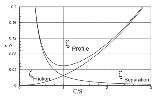
Equation (5.181) exhibits a fundamental relationship between the lift coefficient, the solidity, the inlet and exit flow angle, and the loss coefficient $\zeta$. The question is, how the profile loss $\zeta$ will change if the solidity $\sigma$ changes. The solidity has the major influence on the flow behavior within the blading. If the spacing is too small, the number of blades is large and the friction losses dominate. Increasing the spacing, which is identical to reducing the number of blades, at first causes a reduction of friction losses. Further increasing the spacing decreases the friction losses and also reduces the guidance of the fluid that results in flow separation leading to additional losses. With definite spacing, there is an equilibrium between the separation and friction losses. At this point, the profile loss $\zeta=\zeta_{\text {tnctoon }}+\zeta_{\text {separaton }}$ is at a minimum. The corresponding spacing/chord ratio has an optimum, which is shown in Fig. 5.33. To find the optimum solidity for a variety of turbine and compressor cascades, a series of comprehensive experimental studies have been performed by several researchers. A detailed discussion of the results of these studies is presented in [23].
The relationship for the lift-solidity coefficient derived in the preceding sections is restricted to turbine and compressor stages with constant inner and outer diameters. This geometry is encountered in high pressure turbines or compressor components, where the streamlines are almost parallel to the machine axis. In this special case, the stream surfaces are cylindrical with almost constant diameter. In a general case such as the intermediate and low pressure turbine and compressor stages, however, the stream surfaces have different radii. The meridional velocity component may also change from station to station. In order to calculate the blade lift-solidity coefficient correctly, the radius and the meridional velocity changes must he taken into account. Detailed discussions on this and turbomachinery aero-thermodynamic topics are found in [23].
物理代写|流体力学代写Fluid Mechanics代考|Inviscid Potential Flows
As discussed in Chap. 4 , generally the motion of fluids encountered in engineering applications is described by the Navier-Stokes equations. Considering today’s computational fluid dynamics capabilities, it is possible to numerically solve the Navier-Stokes equations for laminar flows (no turbulent fluctuations), transitional flows (using appropriate intermittency models), and turbulent flow (utilizing appropriate turbulence models). Given today’s computational capabilities, one may argue at this juncture that there is no need to artificially subdivide the flow regime into different categories such as incompressible, compressible, viscid or inviscid ones. However, based on the degree of complexity of the flow under investigation, a computational simulation may take up to several days, weeks, and even months for direct Navier-stokes simulations (DNS). The difficulties associated with solving the Navier-Stokes equations are caused by the existence of the viscosity terms in the Navier-Stokes equations.
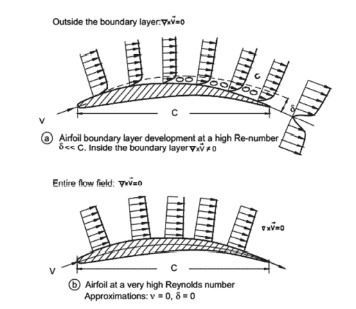
Measuring the velocity distributions encountered in engineering applications such as in a pipe flow, flow around a compressor or turbine blade, or along the wing of an aircraft, we find that the effect of viscosity is confined to a very thin layer called the boundary layer with a local thickness $\delta$. As we discuss in Chap. 11, comprehensive experimental investigations performed earlier by Prandtl $[26,27]$ show that the boundary layer thickness $\delta$ compared to the length $L$ of the subject under investigation is very small. In the vicinity of the wall, because of the no-slip condition, the velocity is $V_{\text {wall }}=0$. Moving away from the wall towards the edge of the boundary layer, the velocity continuously increases until it reaches the velocity at the edge of the boundary layer $V=V_\delta$. Within the boundary layer, the flow is characterized by non-zero vorticity $\nabla \times V \neq 0$. No major changes in velocity magnitude is expected outside the boundary layer, provided that the surface of the subject under investigation does not have a curvature. In case of surfaces with convex or concave curvatures, the velocity outside the boundary layer changes in lateral direction.
Outside the boundary layer, the effect of the viscosity can be neglected as long as the Reynolds number is high enough ( $\operatorname{Re}=100,000$ and above) indicating that the convective flow forces are much larger than the shear stress forces. Theoretically, the boundary layer thickness approaches zero as the Reynolds number tends to infinity. In this case, the flow can be assumed as irrotational, which is then characterized by zero vorticity $\nabla \times V=0$. Thus, as Prandtl suggested, the flow may be decomposed into two distinct regions, the vortical inner region, called the boundary layer, where the viscosity effect is predominant, and the non-vortical region outside the boundary layer.
The flow in the outer region can be calculated using the Euler equation of motion, while the boundary layer method can be applied for calculating the viscous flow within the inner region. Combining these two methods allows calculation of the flow field in a sufficiently accurate manner as long as the boundary layer is not separated. Figure $6.1$ exhibits the velocity distributions along the suction surface of an airfoil. While in case (a) the viscosity is accounted for, in case (b) it is neglected. Thus, the flow is assumed irrotational, which is characterized by $\nabla \times V=0$. As a consequence of this assumption, the velocity on the surface has a non-zero tangential component, which is in contrast to the reality. These type of flows are called potential flows which is the subject of the following sections.
流体力学代写
物理代写|流体力学代写流体力学代考|固体性对叶片型线损失的影响
公式(5.181)给出了升力系数、固体度、进出口流角和损失系数$\zeta$之间的基本关系。问题是,如果坚固度$\sigma$发生变化,配置文件丢失$\zeta$将如何变化。固体度对叶片内部的流动行为有主要影响。如果间隔太小,叶片数量大,摩擦损失占主导地位。增加间距,等同于减少叶片数量,首先会减少摩擦损失。进一步增加间隔会减少摩擦损失,也会减少流体的引导,从而导致流动分离,从而导致额外的损失。在确定间距的情况下,分离和摩擦损失之间存在平衡。此时,配置文件丢失$\zeta=\zeta_{\text {tnctoon }}+\zeta_{\text {separaton }}$处于最小值。相应的间距/弦比有一个最优值,如图5.33所示。为了寻找各种涡轮和压气机叶栅的最佳固体度,许多研究人员进行了一系列综合的实验研究。关于这些研究结果的详细讨论见[23]
前文推导的升力-固度系数关系仅限于内径和外径恒定的涡轮级和压气机级。在高压涡轮或压气机部件中,流线几乎平行于机器轴。在这种特殊情况下,流的表面是圆柱形的,直径几乎恒定。然而,在一般情况下,如中低压涡轮级和压气机级,流面有不同的半径。经向速度分量也可能因站而异。为了正确计算叶片升固系数,必须考虑叶片径向速度和子午速度的变化。关于这和叶轮机械空气-热力学主题的详细讨论见[23]
物理代写|流体力学代写流体力学代考|无粘势流
如第四章所述,工程应用中遇到的流体运动一般用Navier-Stokes方程来描述。考虑到当今的计算流体动力学能力,可以数值求解层流(无湍流涨落)、过渡流(使用适当的间歇模型)和湍流流(使用适当的湍流模型)的Navier-Stokes方程。考虑到今天的计算能力,人们可能会认为没有必要人为地将流动体制细分为不同的类别,如不可压缩、可压缩、粘性或无粘性。然而,根据所研究流体的复杂程度,直接进行Navier-stokes模拟(DNS)可能需要数天、数周甚至数月的时间。与解Navier-Stokes方程相关的困难是由Navier-Stokes方程中粘度项的存在引起的
测量在工程应用中遇到的速度分布,如在管道流动,围绕压气机或涡轮叶片的流动,或沿着飞机的机翼,我们发现粘度的影响仅限于一个非常薄的层称为边界层,局部厚度$\delta$。正如我们在第11章中所讨论的,Prandtl在早期进行的综合实验调查$[26,27]$表明,与被调查对象的长度$L$相比,边界层厚度$\delta$非常小。在墙体附近,由于防滑条件,速度为$V_{\text {wall }}=0$。从壁面向边界层边缘移动,速度不断增加,直到达到边界层边缘的速度$V=V_\delta$。边界层内流动特征为非零涡量$\nabla \times V \neq 0$。只要研究对象的表面没有曲率,预计在边界层外速度大小不会发生重大变化。对于曲率为凸或凹的曲面,边界层外的速度沿横向变化
边界层外,只要雷诺数足够高($\operatorname{Re}=100,000$及以上),表明对流流力远大于剪切应力,粘性的影响可以忽略。理论上,当雷诺数趋于无穷时,边界层厚度趋于零。在这种情况下,可以假定流动为无旋流,其特征为零涡量$\nabla \times V=0$。因此,正如Prandtl所建议的,流动可以被分解为两个不同的区域,一个是内部的涡区,称为边界层,在那里粘度效应是主要的,另一个是非涡区边界层外
外区域的流动可以用欧拉运动方程计算,而内区域的粘性流动可以用边界层法计算。结合这两种方法,只要边界层不分离,流场的计算就足够准确。图$6.1$展示了沿机翼吸力面的速度分布。在(a)情况下考虑了粘度,在(b)情况下忽略了它。因此,假定流为无旋流,其特征为$\nabla \times V=0$。由于这个假设,表面上的速度有一个非零的切向分量,这与实际情况相反。这些类型的流称为势流,这是下面几节的主题

统计代写请认准statistics-lab™. statistics-lab™为您的留学生涯保驾护航。
金融工程代写
金融工程是使用数学技术来解决金融问题。金融工程使用计算机科学、统计学、经济学和应用数学领域的工具和知识来解决当前的金融问题,以及设计新的和创新的金融产品。
非参数统计代写
非参数统计指的是一种统计方法,其中不假设数据来自于由少数参数决定的规定模型;这种模型的例子包括正态分布模型和线性回归模型。
广义线性模型代考
广义线性模型(GLM)归属统计学领域,是一种应用灵活的线性回归模型。该模型允许因变量的偏差分布有除了正态分布之外的其它分布。
术语 广义线性模型(GLM)通常是指给定连续和/或分类预测因素的连续响应变量的常规线性回归模型。它包括多元线性回归,以及方差分析和方差分析(仅含固定效应)。
有限元方法代写
有限元方法(FEM)是一种流行的方法,用于数值解决工程和数学建模中出现的微分方程。典型的问题领域包括结构分析、传热、流体流动、质量运输和电磁势等传统领域。
有限元是一种通用的数值方法,用于解决两个或三个空间变量的偏微分方程(即一些边界值问题)。为了解决一个问题,有限元将一个大系统细分为更小、更简单的部分,称为有限元。这是通过在空间维度上的特定空间离散化来实现的,它是通过构建对象的网格来实现的:用于求解的数值域,它有有限数量的点。边界值问题的有限元方法表述最终导致一个代数方程组。该方法在域上对未知函数进行逼近。[1] 然后将模拟这些有限元的简单方程组合成一个更大的方程系统,以模拟整个问题。然后,有限元通过变化微积分使相关的误差函数最小化来逼近一个解决方案。
tatistics-lab作为专业的留学生服务机构,多年来已为美国、英国、加拿大、澳洲等留学热门地的学生提供专业的学术服务,包括但不限于Essay代写,Assignment代写,Dissertation代写,Report代写,小组作业代写,Proposal代写,Paper代写,Presentation代写,计算机作业代写,论文修改和润色,网课代做,exam代考等等。写作范围涵盖高中,本科,研究生等海外留学全阶段,辐射金融,经济学,会计学,审计学,管理学等全球99%专业科目。写作团队既有专业英语母语作者,也有海外名校硕博留学生,每位写作老师都拥有过硬的语言能力,专业的学科背景和学术写作经验。我们承诺100%原创,100%专业,100%准时,100%满意。
随机分析代写
随机微积分是数学的一个分支,对随机过程进行操作。它允许为随机过程的积分定义一个关于随机过程的一致的积分理论。这个领域是由日本数学家伊藤清在第二次世界大战期间创建并开始的。
时间序列分析代写
随机过程,是依赖于参数的一组随机变量的全体,参数通常是时间。 随机变量是随机现象的数量表现,其时间序列是一组按照时间发生先后顺序进行排列的数据点序列。通常一组时间序列的时间间隔为一恒定值(如1秒,5分钟,12小时,7天,1年),因此时间序列可以作为离散时间数据进行分析处理。研究时间序列数据的意义在于现实中,往往需要研究某个事物其随时间发展变化的规律。这就需要通过研究该事物过去发展的历史记录,以得到其自身发展的规律。
回归分析代写
多元回归分析渐进(Multiple Regression Analysis Asymptotics)属于计量经济学领域,主要是一种数学上的统计分析方法,可以分析复杂情况下各影响因素的数学关系,在自然科学、社会和经济学等多个领域内应用广泛。
MATLAB代写
MATLAB 是一种用于技术计算的高性能语言。它将计算、可视化和编程集成在一个易于使用的环境中,其中问题和解决方案以熟悉的数学符号表示。典型用途包括:数学和计算算法开发建模、仿真和原型制作数据分析、探索和可视化科学和工程图形应用程序开发,包括图形用户界面构建MATLAB 是一个交互式系统,其基本数据元素是一个不需要维度的数组。这使您可以解决许多技术计算问题,尤其是那些具有矩阵和向量公式的问题,而只需用 C 或 Fortran 等标量非交互式语言编写程序所需的时间的一小部分。MATLAB 名称代表矩阵实验室。MATLAB 最初的编写目的是提供对由 LINPACK 和 EISPACK 项目开发的矩阵软件的轻松访问,这两个项目共同代表了矩阵计算软件的最新技术。MATLAB 经过多年的发展,得到了许多用户的投入。在大学环境中,它是数学、工程和科学入门和高级课程的标准教学工具。在工业领域,MATLAB 是高效研究、开发和分析的首选工具。MATLAB 具有一系列称为工具箱的特定于应用程序的解决方案。对于大多数 MATLAB 用户来说非常重要,工具箱允许您学习和应用专业技术。工具箱是 MATLAB 函数(M 文件)的综合集合,可扩展 MATLAB 环境以解决特定类别的问题。可用工具箱的领域包括信号处理、控制系统、神经网络、模糊逻辑、小波、仿真等。