如果你也在 怎样代写宏观经济学Macroeconomics这个学科遇到相关的难题,请随时右上角联系我们的24/7代写客服。
宏观经济学,对国家或地区经济整体行为的研究。它关注的是了解整个经济的事件,如商品和服务的生产总量、失业水平和价格的一般行为。
statistics-lab™ 为您的留学生涯保驾护航 在代写宏观经济学Macroeconomics方面已经树立了自己的口碑, 保证靠谱, 高质且原创的统计Statistics代写服务。我们的专家在代写宏观经济学Macroeconomics代写方面经验极为丰富,各种代写宏观经济学Macroeconomics相关的作业也就用不着说。
我们提供的宏观经济学Macroeconomics及其相关学科的代写,服务范围广, 其中包括但不限于:
- Statistical Inference 统计推断
- Statistical Computing 统计计算
- Advanced Probability Theory 高等概率论
- Advanced Mathematical Statistics 高等数理统计学
- (Generalized) Linear Models 广义线性模型
- Statistical Machine Learning 统计机器学习
- Longitudinal Data Analysis 纵向数据分析
- Foundations of Data Science 数据科学基础
经济代写|宏观经济学代写Macroeconomics代考|The basic mechanics
In its essence, the RBC story goes as follows: consider a positive productivity shock that hits the economy, making it more productive. As a result of that shock, wages (i.e. MPL) and interest rates (i.e. MPK) go up, and individuals want to work more as a result. Because of that, output goes up. It follows that the elasticity of labour supply (and the closely related elasticity of intertemporal substitution) are crucial parameters for RBC models. One can only obtain large fluctuations in employment, as needed to match the data, if this elasticity is sufficiently high. What is the elasticity of labour supply in this basic model? Consider the case when $\frac{(i+r)}{(1+\rho)}=1$, in which consumption is a constant. We can read $(14.8)$ as implying a labour supply curve (a relation between $l_t$ and $w_t$ ):
$$
\phi v^{\prime}\left(1-l_t\right)=\lambda w_t,
$$
where $\lambda$ is the (constant) marginal utility of consumption. Let’s assume a slightly more general, functional form for the utility of leisure:
$$
v(h)=\frac{\sigma}{1-\sigma} h^{\frac{\sigma-1}{\sigma}},
$$
plugging this in (14.15) gives
$$
\phi h_{t^{-\frac{1}{0}}}=\lambda w_t
$$
or
$$
h_t=\left(\frac{\lambda w_t}{\phi}\right)^{-\sigma},
$$
which can be used to compute the labour supply:
$$
l_t=1-\left(\frac{\lambda w_t}{\phi}\right)^{-\sigma} .
$$
This equation has a labour supply elasticity in the short run equal to
$$
\frac{d l}{d w} \frac{w}{l}=\varepsilon_{l, w}=\frac{\sigma\left(\frac{\lambda w_t}{\phi}\right)^{-\sigma-1}\left(\frac{\lambda w_t}{\phi}\right)}{1-\left(\frac{\lambda w_t}{\phi}\right)^{-\sigma}}=\frac{\sigma\left(\frac{\lambda w_t}{\phi}\right)^{-\sigma}}{1-\left(\frac{\lambda w_t}{\phi}\right)^{-\sigma}}=\frac{\sigma h_t}{l_t}
$$
If we assume that $\sigma=1$ (logarithmic utility in leisure), and that $\phi$ and $\lambda$ are such that $\frac{h}{l}=2$ (think about an 8-hour workday), this gives you $\varepsilon_{l, w}=2$. This doesn’t seem to be enough to replicate the employment fluctuations observed in the data. On the other hand, it seems to be quite high if compared to micro data on the elasticity of labour supply. Do you think a decrease of $10 \%$ in real wages (because of inflation, for instance) would lead people to work $20 \%$ fewer hours?
经济代写|宏观经济学代写Macroeconomics代考|The indivisible labour solution
The RBC model thus delivers an elasticity of labour supply that is much higher than what micro evidence suggests, posing a challenge when it comes to matching real-world fluctuations in employment. One proposed solution for the conundrum is to incorporate the fact that labour decisions are often indivisible. This means that people may not make adjustments so much on the intensive margin of hôw mány hours to work in your joob, but moré oftenn on thẻ extensive margin of whéther to work at all. This implies that the aggregate elasticity is large even when the individual elasticity is small.
Hansen (1985) models that by assuming that there are fixed costs of going to work. This can actually make labour supply very responsive for a range of wage levels. The decision variables are both days of work: $d \leq \bar{d}$. and, then, the hours of work each day: $n$. We assume there is a fixed commuting cost in terms of utility $\kappa$, which you pay if you decide to work on that day, regardless of how many hours you work (this would be a sort of commuting time).
The objective function is now
$$
\operatorname{MaxE}\left[\sum_t\left(\frac{1}{1+\rho}\right)^t\left[u\left(c_t\right)-d_t v\left(n_t\right)-\kappa_t d_t\right]\right],
$$
where we leave aside the term $\phi$ to simplify notation, and abuse notation to have $v(\cdot)$ be a function of hours worked, rather than leisure, entering negatively in the utility function. The budget constraint is affected in that now wage income is equal to $w_t d_t n_t$.
It is easy to see that we have the same FOCs, (14.7) – which is unchanged because the terms in consumption in both maximand and budget constraint are still the same -, and (14.8) – because the term in $n_t$ is multiplied by $d_t$ in both maximand and budget constraint, so that $d_t$ cancels out. What changes is that now we have an extra FOC with respect to $d_t$ :
$$
\left[v\left(n_t\right)+k_t\right] \geq u^{\prime}\left(c_t\right) w_t n_t .
$$
Assume $\frac{(1+r)}{(1+\rho)}=1$, so that $c_t$ is constant. Then (14.8) simplifies to
$$
v^{\prime}\left(n_t\right)=\lambda w_t \Longrightarrow n^(w), $$ which gives the optimal amount of hours worked (when the agent decides to work). Then (14.22) simplifies to $$ v\left(n^\right)+k_t \geq \lambda w_t n^* .
$$
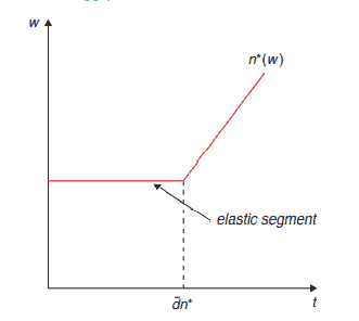
If $v\left(n^\right)+k>\lambda w n^$, then $d=0$, otherwise $d=\bar{d}$. This gives rise to a labour supply as shown in Figure $14.1$
The important point is that this labour supply curve is infinitely elastic at a certain wage. The intuition is that on the margin at which people decide whether to work at all or not, the labour supply will be very sensitive to changes in wages. ${ }^3$
宏观经济学代考
经济代写|宏观经济学代写Macroeconomics代考|The basic mechanics
从本质上讲,RBC 的故事如下:考虑对经济产生积极的生产力冲击,使其更具生产力。由于这种冲击,工资 (即 $\mathrm{MPL}$ ) 和利率 (即 MPK) 上升,因此个人希望工作更多。正因为如此,产量上升。由此可见,劳动力供给 的弹性 (以及密切相关的跨期替代弹性) 是 RBC 模型的关键参数。只有当这种弹性足够高时,才能获得与数据 匹配所需的就业大幅波动。在这个基本模型中,劳动力供给的弹性是多少? 考虑以下情况 $\frac{(i+r)}{(1+\rho)}=1$ ,其中消费 是一个常数。我们可以阅读 $(14.8)$ 作为暗示劳动力供给曲线 (之间的关系 $l_t$ 和 $w_t$ ):
$$
\phi v^{\prime}\left(1-l_t\right)=\lambda w_t,
$$
在哪里 $\lambda$ 是消费的 (不变的) 边际效用。让我们假设休闲效用的更一般的功能形式:
$$
v(h)=\frac{\sigma}{1-\sigma} h^{\frac{\sigma-1}{\sigma}},
$$
将其揷入 (14.15) 给出
$$
\phi h_{t-\frac{1}{0}}=\lambda w_t
$$
或者
$$
h_t=\left(\frac{\lambda w_t}{\phi}\right)^{-\sigma}
$$
可用于计算劳动力供给:
$$
l_t=1-\left(\frac{\lambda w_t}{\phi}\right)^{-\sigma}
$$
这个方程的短期劳动力供给弹性等于
$$
\frac{d l}{d w} \frac{w}{l}=\varepsilon_{l, w}=\frac{\sigma\left(\frac{\lambda w_t}{\phi}\right)^{-\sigma-1}\left(\frac{\lambda w_t}{\phi}\right)}{1-\left(\frac{\lambda w_t}{\phi}\right)^{-\sigma}}=\frac{\sigma\left(\frac{\lambda w_t}{\phi}\right)^{-\sigma}}{1-\left(\frac{\lambda w_t}{\phi}\right)^{-\sigma}}=\frac{\sigma h_t}{l_t}
$$
如果我们假设 $\sigma=1$ (休闲中的对数效用),并且 $\phi$ 和 $\lambda$ 是这样的 $\frac{h}{l}=2$ (想想一个 8 小时的工作日) ,这给了 你 $\varepsilon_{l, w}=2$. 这似乎不足以复制数据中观察到的就业波动。另一方面,如果与劳动力供给弹性的微观数据相比, 它似乎相当高。你认为减少 $10 \%$ 实际工资(例如,由于通货膨胀) 会导致人们工作 $20 \%$ 更少的时间?
经济代写|宏观经济学代写Macroeconomics代考|The indivisible labour solution
因此,RBC 模型提供的劳动力供给弹性远高于微观证据表明的水平,这在匹配现实世界的就业波动方面提出了 挑战。解决这个难题的一种建议是将劳动决策通常是不可分割的事实结合起来。这意味着人们可能不会在你的工 作中工作多少小时的密集边际上做出太多调整,但更经常地在是否工作的广泛边际上做出调整。这意味着即使个 体弹性很小,总体弹性也很大。
Hansen (1985) 通过假设上班有固定成本来建模。这实际上可以使劳动力供应对一系列工资水平非常敏感。决策 变量都是工作天数: $d \leq \bar{d}$. 然后是每天的工作时间: $n$. 我们假设在公用事业方面存在固定的通勤成本 $\kappa$ ,如果 您决定在那一天工作,无论您工作多少小时(这将是一种通勤时间),您都需要支付这笔费用。
现在的目标函数是
$$
\operatorname{MaxE}\left[\sum_t\left(\frac{1}{1+\rho}\right)^t\left[u\left(c_t\right)-d_t v\left(n_t\right)-\kappa_t d_t\right]\right]
$$
我们把这个词放在一边 $\phi$ 简化符号,滥用符号 $v(\cdot)$ 是工作时间的函数,而不是休闲时间,在效用函数中为负数。 预算约束受到影响,因为现在工资收入等于 $w_t d_t n_t$.
很容易看出,我们有相同的 FOC,(14.7) —一它没有改变,因为最大值和预算约束中的消费项仍然相同一— 和 (14.8) —一因为在 $n_t$ 乘以 $d_t$ 在最大约束和预算约束中,所以 $d_t$ 取消。改变的是现在我们有一个额外的 FOC $d_t$ :
$$
\left[v\left(n_t\right)+k_t\right] \geq u^{\prime}\left(c_t\right) w_t n_t
$$
认为 $\frac{(1+r)}{(1+\rho)}=1$ ,以便 $c_t$ 是恒定的。那么 (14.8) 简化为
$$
\left.v^{\prime}\left(n_t\right)=\lambda w_t \Longrightarrow n^{(} w\right)
$$
这给出了最佳的工作时间 (当代理决定工作时)。那么 (14.22) 简化为
vleft(n^1right)+k_t lgeq \ambda w_t $n^{n^{\star}}$ 。
如果 $\vee \backslash l e f t\left(\mathrm{n}^{\wedge} \backslash \mathrm{right}\right)+\mathrm{k}>\backslash \mathrm{ambda} \mathrm{w} \mathrm{n}^{\wedge}$ , 然后 $d=0$ ,否则 $d=\bar{d}$. 这产生了如图所示的劳动力供给 $14.1$
重要的一点是,在一定工资条件下,这条劳动力供给曲线是无限弹性的。直觉是,在人们决定是否工作的边际 上,劳动力供应将对工资的变化非常敏感。

统计代写请认准statistics-lab™. statistics-lab™为您的留学生涯保驾护航。
金融工程代写
金融工程是使用数学技术来解决金融问题。金融工程使用计算机科学、统计学、经济学和应用数学领域的工具和知识来解决当前的金融问题,以及设计新的和创新的金融产品。
非参数统计代写
非参数统计指的是一种统计方法,其中不假设数据来自于由少数参数决定的规定模型;这种模型的例子包括正态分布模型和线性回归模型。
广义线性模型代考
广义线性模型(GLM)归属统计学领域,是一种应用灵活的线性回归模型。该模型允许因变量的偏差分布有除了正态分布之外的其它分布。
术语 广义线性模型(GLM)通常是指给定连续和/或分类预测因素的连续响应变量的常规线性回归模型。它包括多元线性回归,以及方差分析和方差分析(仅含固定效应)。
有限元方法代写
有限元方法(FEM)是一种流行的方法,用于数值解决工程和数学建模中出现的微分方程。典型的问题领域包括结构分析、传热、流体流动、质量运输和电磁势等传统领域。
有限元是一种通用的数值方法,用于解决两个或三个空间变量的偏微分方程(即一些边界值问题)。为了解决一个问题,有限元将一个大系统细分为更小、更简单的部分,称为有限元。这是通过在空间维度上的特定空间离散化来实现的,它是通过构建对象的网格来实现的:用于求解的数值域,它有有限数量的点。边界值问题的有限元方法表述最终导致一个代数方程组。该方法在域上对未知函数进行逼近。[1] 然后将模拟这些有限元的简单方程组合成一个更大的方程系统,以模拟整个问题。然后,有限元通过变化微积分使相关的误差函数最小化来逼近一个解决方案。
tatistics-lab作为专业的留学生服务机构,多年来已为美国、英国、加拿大、澳洲等留学热门地的学生提供专业的学术服务,包括但不限于Essay代写,Assignment代写,Dissertation代写,Report代写,小组作业代写,Proposal代写,Paper代写,Presentation代写,计算机作业代写,论文修改和润色,网课代做,exam代考等等。写作范围涵盖高中,本科,研究生等海外留学全阶段,辐射金融,经济学,会计学,审计学,管理学等全球99%专业科目。写作团队既有专业英语母语作者,也有海外名校硕博留学生,每位写作老师都拥有过硬的语言能力,专业的学科背景和学术写作经验。我们承诺100%原创,100%专业,100%准时,100%满意。
随机分析代写
随机微积分是数学的一个分支,对随机过程进行操作。它允许为随机过程的积分定义一个关于随机过程的一致的积分理论。这个领域是由日本数学家伊藤清在第二次世界大战期间创建并开始的。
时间序列分析代写
随机过程,是依赖于参数的一组随机变量的全体,参数通常是时间。 随机变量是随机现象的数量表现,其时间序列是一组按照时间发生先后顺序进行排列的数据点序列。通常一组时间序列的时间间隔为一恒定值(如1秒,5分钟,12小时,7天,1年),因此时间序列可以作为离散时间数据进行分析处理。研究时间序列数据的意义在于现实中,往往需要研究某个事物其随时间发展变化的规律。这就需要通过研究该事物过去发展的历史记录,以得到其自身发展的规律。
回归分析代写
多元回归分析渐进(Multiple Regression Analysis Asymptotics)属于计量经济学领域,主要是一种数学上的统计分析方法,可以分析复杂情况下各影响因素的数学关系,在自然科学、社会和经济学等多个领域内应用广泛。
MATLAB代写
MATLAB 是一种用于技术计算的高性能语言。它将计算、可视化和编程集成在一个易于使用的环境中,其中问题和解决方案以熟悉的数学符号表示。典型用途包括:数学和计算算法开发建模、仿真和原型制作数据分析、探索和可视化科学和工程图形应用程序开发,包括图形用户界面构建MATLAB 是一个交互式系统,其基本数据元素是一个不需要维度的数组。这使您可以解决许多技术计算问题,尤其是那些具有矩阵和向量公式的问题,而只需用 C 或 Fortran 等标量非交互式语言编写程序所需的时间的一小部分。MATLAB 名称代表矩阵实验室。MATLAB 最初的编写目的是提供对由 LINPACK 和 EISPACK 项目开发的矩阵软件的轻松访问,这两个项目共同代表了矩阵计算软件的最新技术。MATLAB 经过多年的发展,得到了许多用户的投入。在大学环境中,它是数学、工程和科学入门和高级课程的标准教学工具。在工业领域,MATLAB 是高效研究、开发和分析的首选工具。MATLAB 具有一系列称为工具箱的特定于应用程序的解决方案。对于大多数 MATLAB 用户来说非常重要,工具箱允许您学习和应用专业技术。工具箱是 MATLAB 函数(M 文件)的综合集合,可扩展 MATLAB 环境以解决特定类别的问题。可用工具箱的领域包括信号处理、控制系统、神经网络、模糊逻辑、小波、仿真等。