如果你也在 怎样代写风险和利率理论Market Risk, Measures and Portfolio Theory这个学科遇到相关的难题,请随时右上角联系我们的24/7代写客服。
风险度量是历史上预测投资风险和波动的统计措施,它们也是现代投资组合理论(MPT)的主要组成部分。MPT是一种标准的金融和学术方法,用于评估一只股票或一只股票基金与其基准指数相比的表现。
statistics-lab™ 为您的留学生涯保驾护航 在代写风险和利率理论Market Risk, Measures and Portfolio Theory方面已经树立了自己的口碑, 保证靠谱, 高质且原创的统计Statistics代写服务。我们的专家在代写风险和利率理论Market Risk, Measures and Portfolio Theory代写方面经验极为丰富,各种代写风险和利率理论Market Risk, Measures and Portfolio Theory相关的作业也就用不着说。
我们提供的风险和利率理论Market Risk, Measures and Portfolio Theory及其相关学科的代写,服务范围广, 其中包括但不限于:
- Statistical Inference 统计推断
- Statistical Computing 统计计算
- Advanced Probability Theory 高等概率论
- Advanced Mathematical Statistics 高等数理统计学
- (Generalized) Linear Models 广义线性模型
- Statistical Machine Learning 统计机器学习
- Longitudinal Data Analysis 纵向数据分析
- Foundations of Data Science 数据科学基础
金融代写|风险和利率理论代写Market Risk, Measures and Portfolio Theory代考|Semi-variance
Consider the three assets described in Example 1.4. Although $\sigma_1=\sigma_3$, the third asset carries no ‘downside risk’, since neither outcome for $S_3(1)$ involves a loss for the investor. Similarly, although $\sigma_2>\sigma_1$, the downside risk for the second asset is the same as that for the first (a 50\% chance of incurring a loss of 10), but the expected return for the second asset is $15 \%$, making it the more attractive investment even though, as measured by variance, it is more risky. Since investors regard risk as concerned with failure (i.e. downside risk), the following modification of variance is sometimes used. It is called semi-variance and is computed by a formula that takes into account only the unfavourable outcomes, where the return is below the expected value
$$
\mathbb{E}(\min {0, K-\mu})^2 .
$$
The square root of semi-variance is denoted by semi- $\sigma$. However, this notion still does not agree fully with the intuition.
Example $1.6$
Assume that $\Omega=\left{\omega_1, \omega_2\right}, P\left(\left{\omega_1\right}\right)=P\left(\left{\omega_2\right}\right)=\frac{1}{2}$ and
$$
\begin{aligned}
&K\left(\omega_1\right)=10 \%, \
&K\left(\omega_2\right)=20 \% .
\end{aligned}
$$
Consider a modification $K^{\prime}$ with
$$
\begin{aligned}
&K^{\prime}\left(\omega_1\right)=10 \%, \
&K^{\prime}\left(\omega_2\right)=30 \% .
\end{aligned}
$$
Then $K^{\prime}$ is definitely better than $K$ but the semi-variance and the variance for $K^{\prime}$ are both higher than for $K$.
If variance or semi-variance are to represent risk, it is illogical that a better version should be regarded as more risky. This defect can be rectified by replacing the expectation by some other reference point, for instance the risk-free return with the following modification of (1.1),
$$
\mathbb{E}(\min {0, K-R})^2,
$$
which eliminates the above unwanted feature. Instead of the risk-free rate, one can also consider the return required by the investor.
These versions are not very popular in the financial world, the variance being the basic measure of risk. In our presentation of portfolio theory we follow the historical tradition and take variance as the measure of risk. It is possible to develop a version of the theory for alternative ways of measuring risk. In most cases, however, such theories do not produce neat analytic formulae as is the case for the mean and variance.
We will return to a more general discussion of risk measures in the final chapters of this volume. An analysis of the popular concept of Value at Risk (VaR), which has been used extensively in the banking and investment sectors since the 1990s, will lead us to conclude that, despite its ubiquity, this risk measure has serious shortcomings, especially when dealing with mixed distributions. We will then examine an alternative which remedies these defects but still remains mathematically tractable.
金融代写|风险和利率理论代写Market Risk, Measures and Portfolio Theory代考|Portfolios consisting of two assets
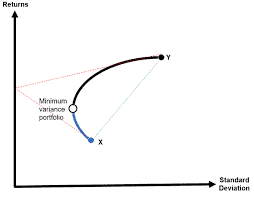
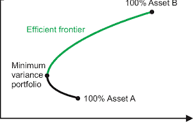
We begin our discussion of portfolio risk and expected return with portfolios consisting of just two securities. This has the advantage that the key concepts of mean-variance portfolio theory can be expressed in simple geometric terms.
For a given allocation of resources between the two assets comprising the portfolio, the mean and variance of the return on the entire portfolio are expressed in terms of the means and variances of, and (crucially) the covariance between, the returns on the individual assets. This enables us to examine the set of all feasible weightings of (in other words, allocations of funds to) the different assets in the portfolio, and to find the unique weighting with minimum variance. We also find the collection of efficient portfolios – ones that are not dominated by any other. Finally, adding a risk-free asset, we find the so-called market portfolio, which is the unique portfolio providing an optimal combination with the risk-free asset.
We denote the prices of the securities as $S_1(t)$ and $S_2(t)$ for $t=0,1$. We start with a motivating example.
Example $2.1$
Let $\Omega=\left{\omega_1, \omega_2\right}, S_1(0)=200, S_2(0)=300$. Assume that
$$
P\left(\left{\omega_1\right}\right)=P\left(\left{\omega_1\right}\right)=\frac{1}{2},
$$
and that
$$
\begin{array}{ll}
S_1\left(1, \omega_1\right)=260, & S_2\left(1, \omega_1\right)=270 \
S_1\left(1, \omega_2\right)=180, & S_2\left(1, \omega_2\right)=360
\end{array}
$$
The expected returns and standard deviations for the two assets are
$$
\begin{array}{ll}
\mu_1=10 \%, & \mu_2=5 \%, \
\sigma_1=20 \%, & \sigma_2=15 \% .
\end{array}
$$
Assume that we spend $V(0)=500$, buying a single share of stock $S_1$ and a single share of stock $S_2$. At time 1 we will have
$$
\begin{aligned}
&V\left(1, \omega_1\right)=260+270=530 \
&V\left(1, \omega_2\right)=180+360=540
\end{aligned}
$$
The expected return on the investment is $7 \%$ and the standard deviation is just $1 \%$. We can see that by diversifying the investment into two stocks we have considerably reduced the risk.
风险和利率理论代写
金融代写|风险和利率理论代写市场风险、度量和投资组合理论代考|半方差
考虑例1.4中描述的三个资产。尽管$\sigma_1=\sigma_3$,第三种资产没有“下行风险”,因为$S_3(1)$的结果都不会给投资者带来损失。同样,尽管第二种资产的下行风险$\sigma_2>\sigma_1$与第一种资产相同(损失为10的概率为50%),但第二种资产的预期回报为$15 \%$,使其成为更有吸引力的投资,尽管根据方差来衡量,它的风险更大。由于投资者认为风险与失败有关(即下行风险),有时使用以下方差修正。它被称为半方差,由一个公式计算,该公式只考虑了不利的结果,其中回报低于期望值
$$
\mathbb{E}(\min {0, K-\mu})^2 .
$$
半方差的平方根用semi- $\sigma$表示。然而,这个概念仍然不完全符合直觉。
示例$1.6$
假设$\Omega=\left{\omega_1, \omega_2\right}, P\left(\left{\omega_1\right}\right)=P\left(\left{\omega_2\right}\right)=\frac{1}{2}$和
$$
\begin{aligned}
&K\left(\omega_1\right)=10 \%, \
&K\left(\omega_2\right)=20 \% .
\end{aligned}
$$
考虑修改$K^{\prime}$与
$$
\begin{aligned}
&K^{\prime}\left(\omega_1\right)=10 \%, \
&K^{\prime}\left(\omega_2\right)=30 \% .
\end{aligned}
$$
那么$K^{\prime}$肯定比$K$好,但$K^{\prime}$的半方差和方差都高于$K$ 如果方差或半方差是用来表示风险的,那么一个更好的版本应该被认为风险更大是不合逻辑的。这一缺陷可以通过将期望替换为其他参考点来纠正,例如对(1.1)进行以下修改的无风险收益,
$$
\mathbb{E}(\min {0, K-R})^2,
$$
消除了上述不需要的特征。除了无风险利率,我们还可以考虑投资者所要求的回报 这些版本在金融界不是很流行,因为方差是风险的基本度量。在我们对投资组合理论的介绍中,我们遵循历史传统,将方差作为风险的度量。为衡量风险的其他方法开发一个理论版本是可能的。然而,在大多数情况下,这类理论并不像均值和方差那样产生简洁的解析公式 我们将在本卷的最后几章回到对风险度量的更一般性的讨论。对自20世纪90年代以来在银行和投资部门广泛使用的流行概念VaR(风险价值)的分析将使我们得出这样的结论:尽管它无处不在,但这种风险度量有严重的缺陷,特别是在处理混合分布时。然后,我们将研究一种补救这些缺陷但在数学上仍可处理的替代方案
金融代写|风险和利率理论代写市场风险、措施和投资组合理论代考|由两种资产组成的投资组合
我们从仅由两种证券组成的投资组合开始讨论投资组合风险和预期收益。这样做的好处是,均值-方差投资组合理论的关键概念可以用简单的几何术语表示 对于组成投资组合的两种资产之间的给定资源配置,整个投资组合的回报率的均值和方差用单个资产回报率的均值和方差以及(至关重要的)两者之间的协方差表示。这使我们能够检查投资组合中不同资产的所有可行权重(换句话说,资金配置)的集合,并找到方差最小的唯一权重。我们还发现了高效投资组合的集合——不受其他任何投资组合支配的组合。最后,添加一个无风险资产,我们得到所谓的市场投资组合,它是提供与无风险资产最优组合的唯一投资组合。
我们将证券的价格表示为$S_1(t)$,将$t=0,1$表示为$S_2(t)$。我们从一个激励的例子开始
示例$2.1$
让$\Omega=\left{\omega_1, \omega_2\right}, S_1(0)=200, S_2(0)=300$。假设
$$
P\left(\left{\omega_1\right}\right)=P\left(\left{\omega_1\right}\right)=\frac{1}{2},
$$$$
\begin{array}{ll}
S_1\left(1, \omega_1\right)=260, & S_2\left(1, \omega_1\right)=270 \
S_1\left(1, \omega_2\right)=180, & S_2\left(1, \omega_2\right)=360
\end{array}
$$
两种资产的预期收益和标准差
$$
\begin{array}{ll}
\mu_1=10 \%, & \mu_2=5 \%, \
\sigma_1=20 \%, & \sigma_2=15 \% .
\end{array}
$$
假设我们花费$V(0)=500$,购买一股股票$S_1$和一股股票$S_2$。在时间1,我们将有
$$
\begin{aligned}
&V\left(1, \omega_1\right)=260+270=530 \
&V\left(1, \omega_2\right)=180+360=540
\end{aligned}
$$
投资的预期回报是$7 \%$,标准差是$1 \%$。我们可以看到,通过将投资分散到两只股票上,我们大大降低了风险

统计代写请认准statistics-lab™. statistics-lab™为您的留学生涯保驾护航。
金融工程代写
金融工程是使用数学技术来解决金融问题。金融工程使用计算机科学、统计学、经济学和应用数学领域的工具和知识来解决当前的金融问题,以及设计新的和创新的金融产品。
非参数统计代写
非参数统计指的是一种统计方法,其中不假设数据来自于由少数参数决定的规定模型;这种模型的例子包括正态分布模型和线性回归模型。
广义线性模型代考
广义线性模型(GLM)归属统计学领域,是一种应用灵活的线性回归模型。该模型允许因变量的偏差分布有除了正态分布之外的其它分布。
术语 广义线性模型(GLM)通常是指给定连续和/或分类预测因素的连续响应变量的常规线性回归模型。它包括多元线性回归,以及方差分析和方差分析(仅含固定效应)。
有限元方法代写
有限元方法(FEM)是一种流行的方法,用于数值解决工程和数学建模中出现的微分方程。典型的问题领域包括结构分析、传热、流体流动、质量运输和电磁势等传统领域。
有限元是一种通用的数值方法,用于解决两个或三个空间变量的偏微分方程(即一些边界值问题)。为了解决一个问题,有限元将一个大系统细分为更小、更简单的部分,称为有限元。这是通过在空间维度上的特定空间离散化来实现的,它是通过构建对象的网格来实现的:用于求解的数值域,它有有限数量的点。边界值问题的有限元方法表述最终导致一个代数方程组。该方法在域上对未知函数进行逼近。[1] 然后将模拟这些有限元的简单方程组合成一个更大的方程系统,以模拟整个问题。然后,有限元通过变化微积分使相关的误差函数最小化来逼近一个解决方案。
tatistics-lab作为专业的留学生服务机构,多年来已为美国、英国、加拿大、澳洲等留学热门地的学生提供专业的学术服务,包括但不限于Essay代写,Assignment代写,Dissertation代写,Report代写,小组作业代写,Proposal代写,Paper代写,Presentation代写,计算机作业代写,论文修改和润色,网课代做,exam代考等等。写作范围涵盖高中,本科,研究生等海外留学全阶段,辐射金融,经济学,会计学,审计学,管理学等全球99%专业科目。写作团队既有专业英语母语作者,也有海外名校硕博留学生,每位写作老师都拥有过硬的语言能力,专业的学科背景和学术写作经验。我们承诺100%原创,100%专业,100%准时,100%满意。
随机分析代写
随机微积分是数学的一个分支,对随机过程进行操作。它允许为随机过程的积分定义一个关于随机过程的一致的积分理论。这个领域是由日本数学家伊藤清在第二次世界大战期间创建并开始的。
时间序列分析代写
随机过程,是依赖于参数的一组随机变量的全体,参数通常是时间。 随机变量是随机现象的数量表现,其时间序列是一组按照时间发生先后顺序进行排列的数据点序列。通常一组时间序列的时间间隔为一恒定值(如1秒,5分钟,12小时,7天,1年),因此时间序列可以作为离散时间数据进行分析处理。研究时间序列数据的意义在于现实中,往往需要研究某个事物其随时间发展变化的规律。这就需要通过研究该事物过去发展的历史记录,以得到其自身发展的规律。
回归分析代写
多元回归分析渐进(Multiple Regression Analysis Asymptotics)属于计量经济学领域,主要是一种数学上的统计分析方法,可以分析复杂情况下各影响因素的数学关系,在自然科学、社会和经济学等多个领域内应用广泛。
MATLAB代写
MATLAB 是一种用于技术计算的高性能语言。它将计算、可视化和编程集成在一个易于使用的环境中,其中问题和解决方案以熟悉的数学符号表示。典型用途包括:数学和计算算法开发建模、仿真和原型制作数据分析、探索和可视化科学和工程图形应用程序开发,包括图形用户界面构建MATLAB 是一个交互式系统,其基本数据元素是一个不需要维度的数组。这使您可以解决许多技术计算问题,尤其是那些具有矩阵和向量公式的问题,而只需用 C 或 Fortran 等标量非交互式语言编写程序所需的时间的一小部分。MATLAB 名称代表矩阵实验室。MATLAB 最初的编写目的是提供对由 LINPACK 和 EISPACK 项目开发的矩阵软件的轻松访问,这两个项目共同代表了矩阵计算软件的最新技术。MATLAB 经过多年的发展,得到了许多用户的投入。在大学环境中,它是数学、工程和科学入门和高级课程的标准教学工具。在工业领域,MATLAB 是高效研究、开发和分析的首选工具。MATLAB 具有一系列称为工具箱的特定于应用程序的解决方案。对于大多数 MATLAB 用户来说非常重要,工具箱允许您学习和应用专业技术。工具箱是 MATLAB 函数(M 文件)的综合集合,可扩展 MATLAB 环境以解决特定类别的问题。可用工具箱的领域包括信号处理、控制系统、神经网络、模糊逻辑、小波、仿真等。