如果你也在 怎样代写偏微分方程partial difference equations这个学科遇到相关的难题,请随时右上角联系我们的24/7代写客服。
偏微分方程指含有未知函数及其偏导数的方程。描述自变量、未知函数及其偏导数之间的关系。符合这个关系的函数是方程的解。
statistics-lab™ 为您的留学生涯保驾护航 在代写偏微分方程partial difference equations方面已经树立了自己的口碑, 保证靠谱, 高质且原创的统计Statistics代写服务。我们的专家在代写偏微分方程partial difference equations代写方面经验极为丰富,各种代写偏微分方程partial difference equations相关的作业也就用不着说。
我们提供的偏微分方程partial difference equations及其相关学科的代写,服务范围广, 其中包括但不限于:
- Statistical Inference 统计推断
- Statistical Computing 统计计算
- Advanced Probability Theory 高等概率论
- Advanced Mathematical Statistics 高等数理统计学
- (Generalized) Linear Models 广义线性模型
- Statistical Machine Learning 统计机器学习
- Longitudinal Data Analysis 纵向数据分析
- Foundations of Data Science 数据科学基础
数学代写|偏微分方程代写partial difference equations代考|CLASSIFICATION OF PDEs
As discussed in the preceding section, at the heart of analysis that utilizes fundamental physics-based principles are differential equations. In the most general case, when the behavior of the system or device is sought as a function of both time and space, the governing equations are PDEs. The solution of a PDE – either by analytical or numerical means – is generally quite complex, and requires a deep understanding of the key attributes of the PDE. These attributes dictate the basic method of solution, how and where boundary and initial conditions must be applied, and what the general nature of the solution is expected to be. Therefore, in this section, we classify PDEs into broad canonical types, and also apply this classification to PDEs commonly encountered in engineering analysis.
We begin our classification by considering a PDE of the following general form:
$$
A \frac{\partial^2 \phi}{\partial x^2}+B \frac{\partial^2 \phi}{\partial x \partial y}+C \frac{\partial^2 \phi}{\partial y^2}+\ldots=0,
$$
where $x$ and $y$ are so-called independent variables, while $\phi$ is the dependent variable. The coefficients $A, B$, and $C$ are either real constants or real functions of the independent or dependent variables. If any of the three coefficients is a function of the dependent variable $\phi$, the PDE becomes nonlinear. Otherwise, it is linear. It is worth pointing out that the distinction between linear and nonlinear PDEs is not related to whether the solution to the PDE is a linear or nonlinear function of $x$ and $y$. As a matter of fact, most linear PDEs yield nonlinear solutions! What matters is whether the PDE has any nonlinearity in the dependent variable $\phi$.
Eq. (1.1) is a PDE in two independent variables. In general, of course, PDEs can be in more than two independent variables, and such scenarios will be discussed in due course. For now, we will restrict ourselves to the bare minimum number of independent variables required to deem a differential equation a PDE. Depending on the values of the coefficients $A, B$, and $C$, PDEs are classified as follows:
If $B^2-4 A C<0$, then the PDE is elliptic. If $B^2-4 A C=0$, then the PDE is parabolic. If $B^2-4 A C>0$, then the PDE is hyperbolic.
Next, we examine a variety of PDEs, commonly encountered in science and engineering disciplines, and use the preceding criteria to identify its type. We begin with the steady-state diffusion equation, written in two independent variables as [2]
$$
\frac{\partial^2 \phi}{\partial x^2}+\frac{\partial^2 \phi}{\partial y^2}=S_\phi,
$$
where $S_\phi$ is the so-called source or source term that, in general, could be a function of either the dependent variables or the independent variables, or both, i.e., $S_\phi=S_\phi(x, y, \phi)$. If the source term is equal to zero, Eq. (1.2) is the so-called Laplace equation. If the source term is a function of the independent variables only, or a constant, i.e., $S_\phi=S_\phi(x, y)$, Eq. (1.2) reduces to the so-called Poisson equation. If the source term is a linear function of the dependent variable, i.e., $S_\phi=a \phi+b$, Eq. (1.2) is referred to as the Helmholtz Equation. The term “diffusion equation” stems from the fact that the differential operators shown in Eq. (1.2) usually arise out of modeling diffusion-like processes such as heat conduction, current conduction, molecular mass diffusion, and other similar phenomena, as is discussed in more detail in Chapters 6 and 7. Irrespective of the aforementioned three forms assumed by Eq. (1.2), comparing it with Eq. (1.1) yields $A=C=1$, and $B=0$, resulting in $B^2-4 A C<0$. Thus, the steady-state diffusion equation, which includes equations of the Laplace, Poisson, or Helmholtz type, is an elliptic PDE. An important characteristic of elliptic PDEs is that they require specification of boundary conditions on all surfaces that bound the domain of solution.
数学代写|偏微分方程代写partial difference equations代考|OVERVIEW OF METHODS FOR SOLVING PDEs
The solution of PDEs is quite challenging. The number of methods available to find closed-form analytical solutions to canonical PDEs is limited. These include separation of variables, superposition, product solution methods, Fourier transforms, Laplace transforms, and perturbation methods, among a few others. Even these methods are limited by constraints such as regular geometry, linearity of the equation, constant coefficients, and others. The imposition of these constraints severely curtails the range of applicability of analytical techniques for solving PDEs, rendering them almost irrelevant for problems of practical interest. In realization of this fact, applied mathematicians and scientists have endeavored to build machines that can solve differential equations by numerical means, as outlined in the brief history of computing presented at the beginning of this chapter.
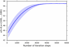
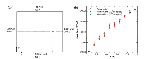
The methods for numerical solution to PDEs can broadly be classified into two types: deterministic and stochastic. A deterministic method is one in which, for a given input to an equation, the output is always the same. The output does not depend on how many times one solves the equation, at what time of the day it is solved, or what computer it is solved on (disregarding precision errors, that may be slightly different on different computers). On the other hand, a stochastic method is based on statistical principles, and the output can be slightly different for the same input depending on how many times the calculation is performed, and other factors. In this case, by “slightly different,” we mean within the statistical error bounds. The difference between these two approaches is best elucidated by a simple example. Let us consider a scenario in which a ball is released from a certain height, $h_i$, above the horizontal ground. Upon collision with the ground, the ball bounces back to a height $h_o$. Let us assume that based on experimental observations or other physical laws, we know that the ball always bounces back to half the height from which it is released. Following this information, we may construct the following deterministic equation: $h_0=(1 / 2) h_i$. If this equation is used to compute the height of a bounced ball, it would always be one-half of the height of release. In other words, the equation (or method of calculation) has one hundred percent confidence built into it. Hence, it is termed a deterministic method. The stochastic viewpoint of the same problem would be quite different. In this viewpoint, one would argue that if $n$ balls were made to bounce, by the laws of theoretical probability, $n / 2$ balls would bounce to a height slightly above half the released height, and the remaining $n / 2$ balls would bounce to a height slightly below the released height, such that in the end, when tallied, the mean height to which the balls bounce back to would be exactly half the height of release. Whether this exact result is recovered or not would depend on how many balls are bounced, i.e., the number of statistical samples used.
偏微分方程代写
数学代写|偏微分方程代写partial difference equations代考|CLASSIFICATION OF PDEs
如前一节所述,利用基于物理的基本原理进行分析的核心是微分方程。在最一般的情况下,当系统或设备的行为被 视为时间和空间的函数时,控制方程是偏微分方程。偏微分方程的解一一无论是通过分析方法还是数值方法一一通 常都非常复杂,需要对偏微分方程的关键属性有深入的了解。这些属性决定了求解的基本方法、边界和初始条件的 应用方式和位置,以及求解的一般性质。因此,在本节中,我们将偏微分方程分类为广泛的规范类型,并将这种分 类应用于工程分析中常见的偏微分方程。
我们通过考虑以下一般形式的 PDE 开始我们的分类:
$$
A \frac{\partial^2 \phi}{\partial x^2}+B \frac{\partial^2 \phi}{\partial x \partial y}+C \frac{\partial^2 \phi}{\partial y^2}+\ldots=0
$$
在哪里 $x$ 和 $y$ 是所谓的自变量,而 $\phi$ 是因变量。系数 $A, B$ ,和 $C$ 是自变量或因变量的实常数或实函数。如果三个系 数中的任何一个是因变量的函数 $\phi$ ,偏微分方程变为非线性。否则,它是线性的。值得指出的是,线性和非线性 PDE 的区别与 PDE 的解是线性函数还是非线性函数无关 $x$ 和 $y$. 事实上,大多数线性 PDE 都会产生非线性解! 重要 的是 PDE 在因变量中是否有任何非线性 $\phi$.
方程。(1.1) 是两个自变量的偏微分方程。当然,一般来说,偏微分方程可以包含两个以上的自变量,这些情况将 在适当的时候讨论。现在,我们将限制在将溦分方程视为 PDE所需的最小自变量数。取决于系数的值 $A, B$ ,和 $C$ ,偏微分方程分类如下:
如果 $B^2-4 A C<0$ ,则 PDE 是椭圆的。如果 $B^2-4 A C=0$ ,则 PDE 是抛物线的。如果 $B^2-4 A C>0$ ,则 PDE 是双曲线的。
接下来,我们检查在科学和工程学科中常见的各种 PDE,并使用前面的标准来识别其类型。我们从稳态扩散方程 开始,用两个自变量写成 [2]
$$
\frac{\partial^2 \phi}{\partial x^2}+\frac{\partial^2 \phi}{\partial y^2}=S_\phi,
$$
在哪里 $S_\phi$ 是所谓的源或源项,一般来说,它可以是因变量或自变量或两者的函数,即 $S_\phi=S_\phi(x, y, \phi)$. 如果源 项等于零,则方程。(1.2) 就是所谓的拉普拉斯方程。如果源项仅是自变量的函数,或者是一个常数,即 $S_\phi=S_\phi(x, y)$, 方程。 $(1.2)$ 式简化为所谓的泊松方程。如果源项是因变量的线性函数,即 $S_\phi=a \phi+b$ ,方 程。(1.2) 被称为亥姆霍兹方程。术语“扩散方程”源于方程中显示的微分算子这一事实。 (1.2) 式通常源于对类似 扩散的过程进行建模,例如热传导、电流传导、分子质量扩散和其他类似现象,如第 6 章和第 7 章中更详细讨论 的那样。无论公式中假设的上述三种形式如何. (1.2),将其与等式比较。(1.1)产量 $A=C=1$ ,和 $B=0$ , 导致 $B^2-4 A C<0$. 因此,包括 Laplace、Poisson 或 Helmholtz 类型方程的稳态扩散方程是椭圆 PDE。椭圆 偏微分方程的一个重要特征是它们需要在所有限定解域的表面上指定边界条件。
数学代写|偏微分方程代写partial difference equations代考|OVERVIEW OF METHODS FOR SOLVING PDEs
PDE 的求解非常具有挑战性。可用于找到典型 PDE 的封闭式解析解的方法数量有限。其中包括变量分离、叠加、乘积求解方法、傅里叶变换、拉普拉斯变换和微扰方法等。即使这些方法也受到诸如规则几何、方程线性、常数系数等约束的限制。这些约束的强加严重限制了分析技术在求解偏微分方程中的适用范围,使得它们几乎与实际感兴趣的问题无关。为了实现这一事实,应用数学家和科学家们努力制造可以通过数值方法求解微分方程的机器,
偏微分方程的数值求解方法大致可分为两种类型:确定性和随机性。确定性方法是这样一种方法,对于给定的方程输入,输出总是相同的。输出不取决于求解方程的次数、求解的时间或求解的计算机(不考虑精度误差,在不同的计算机上可能略有不同)。另一方面,随机方法基于统计原理,对于相同的输入,输出可能会略有不同,具体取决于执行计算的次数和其他因素。在这种情况下,“略有不同”是指在统计误差范围内。这两种方法之间的区别最好通过一个简单的例子来说明。H一世,高于水平地面。与地面碰撞后,球弹回一个高度H○. 让我们假设根据实验观察或其他物理定律,我们知道球总是弹回它被释放的高度的一半。根据这些信息,我们可以构建以下确定性方程:H0=(1/2)H一世. 如果用这个方程来计算弹跳球的高度,它总是释放高度的二分之一。换句话说,方程(或计算方法)内置了百分百的置信度。因此,它被称为确定性方法。同一个问题的随机观点会完全不同。在这种观点下,有人会争辩说,如果n根据理论概率定律,球会反弹,n/2球会反弹到略高于释放高度一半的高度,剩下的n/2球会反弹到略低于释放高度的高度,这样最终,当计算时,球反弹到的平均高度将恰好是释放高度的一半。这个准确的结果是否被恢复将取决于有多少球被反弹,即使用的统计样本的数量。

统计代写请认准statistics-lab™. statistics-lab™为您的留学生涯保驾护航。
金融工程代写
金融工程是使用数学技术来解决金融问题。金融工程使用计算机科学、统计学、经济学和应用数学领域的工具和知识来解决当前的金融问题,以及设计新的和创新的金融产品。
非参数统计代写
非参数统计指的是一种统计方法,其中不假设数据来自于由少数参数决定的规定模型;这种模型的例子包括正态分布模型和线性回归模型。
广义线性模型代考
广义线性模型(GLM)归属统计学领域,是一种应用灵活的线性回归模型。该模型允许因变量的偏差分布有除了正态分布之外的其它分布。
术语 广义线性模型(GLM)通常是指给定连续和/或分类预测因素的连续响应变量的常规线性回归模型。它包括多元线性回归,以及方差分析和方差分析(仅含固定效应)。
有限元方法代写
有限元方法(FEM)是一种流行的方法,用于数值解决工程和数学建模中出现的微分方程。典型的问题领域包括结构分析、传热、流体流动、质量运输和电磁势等传统领域。
有限元是一种通用的数值方法,用于解决两个或三个空间变量的偏微分方程(即一些边界值问题)。为了解决一个问题,有限元将一个大系统细分为更小、更简单的部分,称为有限元。这是通过在空间维度上的特定空间离散化来实现的,它是通过构建对象的网格来实现的:用于求解的数值域,它有有限数量的点。边界值问题的有限元方法表述最终导致一个代数方程组。该方法在域上对未知函数进行逼近。[1] 然后将模拟这些有限元的简单方程组合成一个更大的方程系统,以模拟整个问题。然后,有限元通过变化微积分使相关的误差函数最小化来逼近一个解决方案。
tatistics-lab作为专业的留学生服务机构,多年来已为美国、英国、加拿大、澳洲等留学热门地的学生提供专业的学术服务,包括但不限于Essay代写,Assignment代写,Dissertation代写,Report代写,小组作业代写,Proposal代写,Paper代写,Presentation代写,计算机作业代写,论文修改和润色,网课代做,exam代考等等。写作范围涵盖高中,本科,研究生等海外留学全阶段,辐射金融,经济学,会计学,审计学,管理学等全球99%专业科目。写作团队既有专业英语母语作者,也有海外名校硕博留学生,每位写作老师都拥有过硬的语言能力,专业的学科背景和学术写作经验。我们承诺100%原创,100%专业,100%准时,100%满意。
随机分析代写
随机微积分是数学的一个分支,对随机过程进行操作。它允许为随机过程的积分定义一个关于随机过程的一致的积分理论。这个领域是由日本数学家伊藤清在第二次世界大战期间创建并开始的。
时间序列分析代写
随机过程,是依赖于参数的一组随机变量的全体,参数通常是时间。 随机变量是随机现象的数量表现,其时间序列是一组按照时间发生先后顺序进行排列的数据点序列。通常一组时间序列的时间间隔为一恒定值(如1秒,5分钟,12小时,7天,1年),因此时间序列可以作为离散时间数据进行分析处理。研究时间序列数据的意义在于现实中,往往需要研究某个事物其随时间发展变化的规律。这就需要通过研究该事物过去发展的历史记录,以得到其自身发展的规律。
回归分析代写
多元回归分析渐进(Multiple Regression Analysis Asymptotics)属于计量经济学领域,主要是一种数学上的统计分析方法,可以分析复杂情况下各影响因素的数学关系,在自然科学、社会和经济学等多个领域内应用广泛。
MATLAB代写
MATLAB 是一种用于技术计算的高性能语言。它将计算、可视化和编程集成在一个易于使用的环境中,其中问题和解决方案以熟悉的数学符号表示。典型用途包括:数学和计算算法开发建模、仿真和原型制作数据分析、探索和可视化科学和工程图形应用程序开发,包括图形用户界面构建MATLAB 是一个交互式系统,其基本数据元素是一个不需要维度的数组。这使您可以解决许多技术计算问题,尤其是那些具有矩阵和向量公式的问题,而只需用 C 或 Fortran 等标量非交互式语言编写程序所需的时间的一小部分。MATLAB 名称代表矩阵实验室。MATLAB 最初的编写目的是提供对由 LINPACK 和 EISPACK 项目开发的矩阵软件的轻松访问,这两个项目共同代表了矩阵计算软件的最新技术。MATLAB 经过多年的发展,得到了许多用户的投入。在大学环境中,它是数学、工程和科学入门和高级课程的标准教学工具。在工业领域,MATLAB 是高效研究、开发和分析的首选工具。MATLAB 具有一系列称为工具箱的特定于应用程序的解决方案。对于大多数 MATLAB 用户来说非常重要,工具箱允许您学习和应用专业技术。工具箱是 MATLAB 函数(M 文件)的综合集合,可扩展 MATLAB 环境以解决特定类别的问题。可用工具箱的领域包括信号处理、控制系统、神经网络、模糊逻辑、小波、仿真等。