如果你也在 怎样代写回归分析Regression Analysis这个学科遇到相关的难题,请随时右上角联系我们的24/7代写客服。
回归分析是一种强大的统计方法,允许你检查两个或多个感兴趣的变量之间的关系。虽然有许多类型的回归分析,但它们的核心都是考察一个或多个自变量对因变量的影响。
statistics-lab™ 为您的留学生涯保驾护航 在代写回归分析Regression Analysis方面已经树立了自己的口碑, 保证靠谱, 高质且原创的统计Statistics代写服务。我们的专家在代写回归分析Regression Analysis代写方面经验极为丰富,各种代写回归分析Regression Analysis相关的作业也就用不着说。
我们提供的回归分析Regression Analysis及其相关学科的代写,服务范围广, 其中包括但不限于:
- Statistical Inference 统计推断
- Statistical Computing 统计计算
- Advanced Probability Theory 高等楖率论
- Advanced Mathematical Statistics 高等数理统计学
- (Generalized) Linear Models 广义线性模型
- Statistical Machine Learning 统计机器学习
- Longitudinal Data Analysis 纵向数据分析
- Foundations of Data Science 数据科学基础
统计代写|回归分析作业代写Regression Analysis代考|Evaluating the Linearity Assumption Using Graphical Methods
While we are not big fans of data analysis “recipes,” in regression or elsewhere, which instruct you to perform step 1, step 2, step 3, etc. for the analysis of your data, we are happy to recommend the following first step for the analysis of regression data.
Step 1 of any analysis of regression data
Plot the ordinary $\left(x_i, y_i\right)$ scatterplot, or scatterplots if there are multiple $X$ variables.
The simple $\left(x_i, y_i\right)$ scatterplot gives you immediate insight into the viability of the linearity, constant variance, and normality assumptions (see Section $1.8$ for examples of such scatterplots). It will also alert you to the presence of outliers.
To evaluate linearity using the $\left(x_i, y_i\right)$ scatterplot, simply look for evidence of curvature. You can overlay the LOESS fit to better estimate the form of the curvature. Recall, though, that all assumptions refer to the data-generating process. Thus, if you are going to claim there is curvature, such curvature should make sense in the context of the subject matter. For one example, boundary constraints can force curvature: If the minimum $Y$ is zero, then the curve must flatten for $X$ values where $Y$ is close to zero. For another example, in the case of the product preference vs. product complexity shown in Figure 1.16, there is a subject matter rationale for the curvature: People prefer more complexity up to a point, after which more complexity is less desirable. Ideally, you should be able to justify curvature in terms of the processes that produced your data.
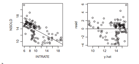
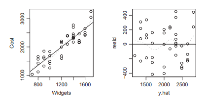
A refinement of the $\left(x_i, y_i\right)$ scatterplot is the residual $\left(x_i, e_i\right)$ scatterplot. This scatterplot is an alternative, “magnified” view of the $\left(x_i, y_i\right)$ scatterplot, where the $e=0$ horizontal line in the $\left(x_i, e_i\right)$ scatterplot corresponds to the least-squares line in the $\left(x_i, y_i\right)$ scatterplot. Look for upward or downward ” $\mathrm{U}^{\prime \prime}$ shape to suggest curvature; overlay the LOESS fit to the $\left(x_i, e_i\right)$ data to help see these patterns.
You can also use the $\left(\hat{y}i, e_i\right)$ scatterplot to check the linearity assumption. In simple regression (i.e., one $X$ variable), the $\left(\hat{y}_i, e_i\right)$ scatterplot is identical to the $\left(x_i, e_i\right)$ scatterplot, with the exception that the horizontal scale is linearly transformed via $\hat{y}_i=\hat{\beta}_0+\hat{\beta}_1 x_i$. When the estimated slope is negative, the horizontal axis is “reflected”-large values of $x$ map to small values of $\hat{y}_i$ and vice versa. You can use this plot just like the $\left(x_i, e_i\right)$ scatterplot. In simple regression, the $\left(\hat{y}_i, e_i\right)$ scatterplot offers no advantage over the $\left(x_i, e_i\right)$ scatterplot. However, in multiple regression, the $\left(\hat{y}_i, e_i\right)$ scatterplot is invaluable as a quick look at the overall model, since there is just one $\left(\hat{y}_i, e_i\right)$ plot to look at, instead of several $\left(x{i j}, e_i\right)$ plots (one for each $X_j$ variable). This $\left(\hat{y}_i, e_i\right)$ scatterplot, which you can call a “predicted/residual scatterplot,” is automatically provided by $\mathrm{R}$ when you plot a fitted lm object.
统计代写|回归分析作业代写Regression Analysis代考|Evaluating the Linearity Assumption Using Hypothesis Testing Methods
Here, we will get slightly ahead of the flow of the book, because multiple regression is covered in the next chapter. A simple, powerful way to test for curvature is to use a multiple regression model that includes a quadratic term. The quadratic regression model is given by:
$$
Y=\beta_0+\beta_1 X+\beta_2 X^2+\varepsilon
$$
This model assumes that, if there is curvature, then it takes a quadratic form. Logic for making this assumption is given by “Taylor’s Theorem,” which states that many types of curved functions are well approximated by quadratic functions.
Testing methods require restricted (null) and unrestricted (alternative) models. Here, the null model enforces the restriction that $\beta_2=0$; thus the null model states that the mean response is a linear (not curved) function of $x$. So-called “insignificance” (determined historically by $p>0.05$ ) of the estimate of $\beta_2$ means that the evidence of curvature in the observed data, as indicated by a non-zero estimate of $\beta_2$ or by a curved LOESS fit, is explainable by chance alone under the linear model. “Significance” (determined historically by $p<0.05$ ) means that such evidence of curvature is not easily explained by chance alone under the linear model.
But you should not take the result of this $p$-value based test as a “recipe” for model construction. If “significant,” you should not automatically assume a curved model. Instead, you should ask, “Is the curvature dramatic enough to warrant the additional modeling complexity?” and “Do the predictions differ much, whether you use a model for curvature or the ordinary linear model?” If the answers to those questions are “No,” then you should use the linear model anyway, even if it was “rejected” by the $p$-value based test.
In addition, models employing curvature (particularly quadratics) are notoriously poor at the extremes of the $x$-range(s). So again, you can easily prefer the linear model, even if the curvature is “significant” $(p<0.05)$.
Conversely, if the quadratic term is “insignificant,” it does not mean that the function is linear. Recall from Chapter 1 that the linearity is usually false, a priori; hence, “insignificance” means that you have failed to detect curvature. If the test for the quadratic term is “insignificant,” it is most likely a Type II error.
Even when the curvature does not have a perfectly quadratic form, the quadratic test is usually very powerful; rare exceptions include cases where the curvature is somewhat exotic. If the quadratic model is grossly wrong for modeling curvature in your application, then you should use a test based on a model other than the quadratic model.
回归分析代写
统计代写|回归分析作业代写Regression Analysis代考|Evaluating the Linearity Assumption Using Graphical Methods
虽然我们不是回归或其他地方的数据分析“食谱”的忠实拥护者,它们会指导您执行第 1 步、第 2 步、第 3 步等来分析您的数据,但我们很乐意推荐以下第一步用于分析回归数据。
任何回归数据分析的步骤 1
绘制普通图(X一世,是一世)散点图,或散点图(如果有多个)X变量。
简单的(X一世,是一世)散点图可让您立即了解线性、恒定方差和正态假设的可行性(参见第1.8有关此类散点图的示例)。它还会提醒您注意异常值的存在。
使用(X一世,是一世)散点图,只需寻找曲率的证据。您可以叠加 LOESS 拟合以更好地估计曲率的形式。但请回想一下,所有假设都涉及数据生成过程。因此,如果您要声称存在曲率,那么这种曲率在主题的上下文中应该是有意义的。例如,边界约束可以强制曲率:如果最小值是为零,则曲线必须变平X值在哪里是接近于零。再举一个例子,在图 1.16 所示的产品偏好与产品复杂性的情况下,曲率有一个主题基本原理:人们在某一点上更喜欢更复杂的东西,之后更不想要更多的复杂性。理想情况下,您应该能够根据产生数据的过程来证明曲率是合理的。
的细化(X一世,是一世)散点图是残差(X一世,和一世)散点图。这个散点图是另一种“放大”视图(X一世,是一世)散点图,其中和=0中的水平线(X一世,和一世)散点图对应于(X一世,是一世)散点图。向上或向下寻找”在′′形状暗示曲率;覆盖黄土适合(X一世,和一世)数据以帮助查看这些模式。
您还可以使用(是^一世,和一世)散点图检查线性假设。在简单回归中(即,一个X变量),(是^一世,和一世)散点图与(X一世,和一世)散点图,除了水平刻度通过线性变换是^一世=b^0+b^1X一世. 当估计的斜率为负时,水平轴是“反映”的——大的值X映射到小的值是^一世反之亦然。你可以像使用这个情节一样(X一世,和一世)散点图。在简单回归中,(是^一世,和一世)散点图没有任何优势(X一世,和一世)散点图。然而,在多元回归中,(是^一世,和一世)散点图对于快速查看整个模型非常有用,因为只有一个(是^一世,和一世)情节看,而不是几个(X一世j,和一世)地块(每个一个Xj多变的)。这个(是^一世,和一世)散点图,您可以称之为“预测/残差散点图”,由R当您绘制拟合的 lm 对象时。
统计代写|回归分析作业代写Regression Analysis代考|Evaluating the Linearity Assumption Using Hypothesis Testing Methods
在这里,我们将稍微领先于本书的流程,因为下一章将介绍多元回归。测试曲率的一种简单而有效的方法是使用 包含二次项的多元回归模型。二次回归模型由下式给出:
$$
Y=\beta_0+\beta_1 X+\beta_2 X^2+\varepsilon
$$
该模型假设,如果存在曲率,则它采用二次形式。做出这种假设的逻辑由“泰勒定理”给出,该定理指出许多类型的 曲线函数可以很好地近似于二次函数。
测试方法需要受限 (null) 和非受限(替代)模型。在这里,空模型强制执行以下限制: $\beta_2=0$; 因此,空模型表 明平均响应是线性 (非曲线) 函数 $x$. 所谓的”微不足道” (历史上由 $p>0.05$ ) 的估计 $\beta_2$ 表示观测数据中存在曲率 的证据,如非零估计所示 $\beta_2$ 或通过弯曲的 LOESS 拟合,在线性模型下仅靠偶然性可以解释。“意义” (历史上由 $p<0.05)$ 意味着在线性模型下,这种曲率的证据很难仅靠偶然性来解释。
但是你不应该接受这个结果 $p$ 基于价值的测试作为模型构建的“秘诀”。如果“显着”,则不应自动假定为弯曲模型。 相反,您应该问: “曲率是否足以保证额外的建模复杂性? “和“无论您使用曲率模型还是普通线性模型,预测是否 有很大差异? “如果这些问题的答案是“否”,那么您无论如何都应该使用线性模型,即使它被 $p$-基于价值的测试。
此外,使用曲率 (特别是二次方) 的模型在 $x$-范围。因此,即使曲率“显着”,您也可以轻松地选择线性模型 $(p<0.05)$
相反,如果二次项“无关紧要”,则并不意味着该函数是线性的。回想一下第 1 章,线性通常是错误的,先验的;因 此,”无意义”意味着您末能检测到曲率。如果对二次项的检验”不显着”,则很可能是 II 类错误。
即使曲率没有完美的二次形式,二次检验通常也很有效;极少数例外情况包括曲率有些奇异的情况。如果二次模 型在您的应用程序中对曲率建模严重错误,那么您应该使用基于二次模型以外的模型的测试。

统计代写请认准statistics-lab™. statistics-lab™为您的留学生涯保驾护航。
随机过程代考
在概率论概念中,随机过程是随机变量的集合。 若一随机系统的样本点是随机函数,则称此函数为样本函数,这一随机系统全部样本函数的集合是一个随机过程。 实际应用中,样本函数的一般定义在时间域或者空间域。 随机过程的实例如股票和汇率的波动、语音信号、视频信号、体温的变化,随机运动如布朗运动、随机徘徊等等。
贝叶斯方法代考
贝叶斯统计概念及数据分析表示使用概率陈述回答有关未知参数的研究问题以及统计范式。后验分布包括关于参数的先验分布,和基于观测数据提供关于参数的信息似然模型。根据选择的先验分布和似然模型,后验分布可以解析或近似,例如,马尔科夫链蒙特卡罗 (MCMC) 方法之一。贝叶斯统计概念及数据分析使用后验分布来形成模型参数的各种摘要,包括点估计,如后验平均值、中位数、百分位数和称为可信区间的区间估计。此外,所有关于模型参数的统计检验都可以表示为基于估计后验分布的概率报表。
广义线性模型代考
广义线性模型(GLM)归属统计学领域,是一种应用灵活的线性回归模型。该模型允许因变量的偏差分布有除了正态分布之外的其它分布。
statistics-lab作为专业的留学生服务机构,多年来已为美国、英国、加拿大、澳洲等留学热门地的学生提供专业的学术服务,包括但不限于Essay代写,Assignment代写,Dissertation代写,Report代写,小组作业代写,Proposal代写,Paper代写,Presentation代写,计算机作业代写,论文修改和润色,网课代做,exam代考等等。写作范围涵盖高中,本科,研究生等海外留学全阶段,辐射金融,经济学,会计学,审计学,管理学等全球99%专业科目。写作团队既有专业英语母语作者,也有海外名校硕博留学生,每位写作老师都拥有过硬的语言能力,专业的学科背景和学术写作经验。我们承诺100%原创,100%专业,100%准时,100%满意。
机器学习代写
随着AI的大潮到来,Machine Learning逐渐成为一个新的学习热点。同时与传统CS相比,Machine Learning在其他领域也有着广泛的应用,因此这门学科成为不仅折磨CS专业同学的“小恶魔”,也是折磨生物、化学、统计等其他学科留学生的“大魔王”。学习Machine learning的一大绊脚石在于使用语言众多,跨学科范围广,所以学习起来尤其困难。但是不管你在学习Machine Learning时遇到任何难题,StudyGate专业导师团队都能为你轻松解决。
多元统计分析代考
基础数据: $N$ 个样本, $P$ 个变量数的单样本,组成的横列的数据表
变量定性: 分类和顺序;变量定量:数值
数学公式的角度分为: 因变量与自变量
时间序列分析代写
随机过程,是依赖于参数的一组随机变量的全体,参数通常是时间。 随机变量是随机现象的数量表现,其时间序列是一组按照时间发生先后顺序进行排列的数据点序列。通常一组时间序列的时间间隔为一恒定值(如1秒,5分钟,12小时,7天,1年),因此时间序列可以作为离散时间数据进行分析处理。研究时间序列数据的意义在于现实中,往往需要研究某个事物其随时间发展变化的规律。这就需要通过研究该事物过去发展的历史记录,以得到其自身发展的规律。
回归分析代写
多元回归分析渐进(Multiple Regression Analysis Asymptotics)属于计量经济学领域,主要是一种数学上的统计分析方法,可以分析复杂情况下各影响因素的数学关系,在自然科学、社会和经济学等多个领域内应用广泛。
MATLAB代写
MATLAB 是一种用于技术计算的高性能语言。它将计算、可视化和编程集成在一个易于使用的环境中,其中问题和解决方案以熟悉的数学符号表示。典型用途包括:数学和计算算法开发建模、仿真和原型制作数据分析、探索和可视化科学和工程图形应用程序开发,包括图形用户界面构建MATLAB 是一个交互式系统,其基本数据元素是一个不需要维度的数组。这使您可以解决许多技术计算问题,尤其是那些具有矩阵和向量公式的问题,而只需用 C 或 Fortran 等标量非交互式语言编写程序所需的时间的一小部分。MATLAB 名称代表矩阵实验室。MATLAB 最初的编写目的是提供对由 LINPACK 和 EISPACK 项目开发的矩阵软件的轻松访问,这两个项目共同代表了矩阵计算软件的最新技术。MATLAB 经过多年的发展,得到了许多用户的投入。在大学环境中,它是数学、工程和科学入门和高级课程的标准教学工具。在工业领域,MATLAB 是高效研究、开发和分析的首选工具。MATLAB 具有一系列称为工具箱的特定于应用程序的解决方案。对于大多数 MATLAB 用户来说非常重要,工具箱允许您学习和应用专业技术。工具箱是 MATLAB 函数(M 文件)的综合集合,可扩展 MATLAB 环境以解决特定类别的问题。可用工具箱的领域包括信号处理、控制系统、神经网络、模糊逻辑、小波、仿真等。