statistics-lab™ 为您的留学生涯保驾护航在代写回归分析Regression Analysis方面已经树立了自己的口碑, 保证靠谱, 高质且原创的统计Statistics代写服务。我们的专家在代写回归分析Regression Analysis代写方面经验极为丰富，各种代写回归分析Regression Analysis相关的作业也就用不着说。

统计代写|回归分析作业代写Regression Analysis代考|Evaluating the Linearity Assumption Using Hypothesis Testing Methods

Here, we will get slightly ahead of the flow of the book, because multiple regression is covered in the next chapter. A simple, powerful way to test for curvature is to use a multiple regression model that includes a quadratic term. The quadratic regression model is given by:
$$
Y=\beta_0+\beta_1 X+\beta_2 X^2+\varepsilon
$$
This model assumes that, if there is curvature, then it takes a quadratic form. Logic for making this assumption is given by “Taylor’s Theorem,” which states that many types of curved functions are well approximated by quadratic functions.

Testing methods require restricted (null) and unrestricted (alternative) models. Here, the null model enforces the restriction that $\beta_2=0$; thus the null model states that the mean response is a linear (not curved) function of $x$. So-called “insignificance” (determined historically by $p>0.05$ ) of the estimate of $\beta_2$ means that the evidence of curvature in the observed data, as indicated by a non-zero estimate of $\beta_2$ or by a curved LOESS fit, is explainable by chance alone under the linear model. “Significance” (determined historically by $p<0.05$ ) means that such evidence of curvature is not easily explained by chance alone under the linear model.

But you should not take the result of this $p$-value based test as a “recipe” for model construction. If “significant,” you should not automatically assume a curved model. Instead, you should ask, “Is the curvature dramatic enough to warrant the additional modeling complexity?” and “Do the predictions differ much, whether you use a model for curvature or the ordinary linear model?” If the answers to those questions are “No,” then you should use the linear model anyway, even if it was “rejected” by the $p$-value based test.

In addition, models employing curvature (particularly quadratics) are notoriously poor at the extremes of the $x$-range(s). So again, you can easily prefer the linear model, even if the curvature is “significant” $(p<0.05)$.

统计代写|回归分析作业代写Regression Analysis代考|Testing for Curvature with the Production Cost Data

The following R code illustrates the method.
ProdC $=$ read.table(“https://raw.githubusercontent.com/andrea2719/
URA-DataSets/master/ProdC.txt”)
attach(ProdC)
plot (Widgets, Cost); abline(lsfit(Widgets, Cost))
Widgets.squared = Widgets^2
Prodc $=$ read.table $($ “https $: / /$ raw.githubusercontent.com/andrea2719/
URA-Datasets/master/ProdC.txt”)
attach (ProdC)
plot (Widgets, Cost); abline(lsfit(Widgets, Cost))
Widgets.squared $=$ Widgets $^{\wedge} 2$

fit.quad $=1 \mathrm{~m}$ (Cost $~$ Widgets + Widgets.squared); summary (fit.quad)
lines(spline(Widgets, predict(fit.quad)), col = “gray”, lty=2)
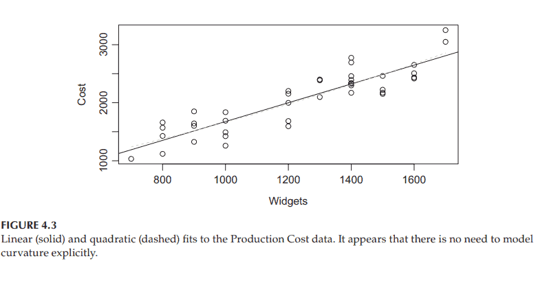
Figure 4.3 shows both the linear and quadratic (curved) fit to the data. Since the linear and quadratic fits are so similar, it (again) appears that there is no need to model the curvature explicitly in this example.
Relevant lines from the summary of fit are shown as follows:
Coefficients :
(Intercept)
widgets
Widgets.squared
$\begin{array}{cccc}\text { Estimate } & \text { Std. Error } & t \text { value } & \operatorname{Pr}(>|t|) \ 4.564 e+02 & 7.493 e+02 & 0.609 & 0.546 \ 9.149 e-01 & 1.290 e+00 & 0.709 & 0.483 \ 2.923 e-04 & 5.322 e-04 & 0.549 & 0.586\end{array}$
Residual standard error: 241.3 on 37 degrees of freedom
Multiple R-squared: 0.7987 , Adjusted R-squared: 0.7878
F-statistic: 73.42 on 2 and $37 \mathrm{DF}$, p-value: $1.318 \mathrm{e}-13$
Notice the $p$-value for testing the $\beta_2=0$ restriction: Since the $p$-value is 0.586 , the difference between the coefficient 0.0002923 (2.923e-04) and 0.0 is explainable by chance alone. That is, even if the process were truly linear (i.e., even if $\beta_2=0$ ), you would often see quadratic coefficient estimates $\left(\hat{\beta}_2\right)$ as large as 0.0002923 when you fit a quadratic model to similar data. If this is confusing to you, just run a simulation from a similar linear process (where $\beta_2=0$ ), and fit a quadratic model. You will see a non-zero $\hat{\beta}_2$ in every simulated data set, and most will be within 2 standard errors of 0.0 (the $\hat{\beta}_2$ above is $T=0.549$ standard errors from 0.0 ).

回归分析代写

统计代写|回归分析作业代写Regression Analysis代考|Evaluating the Linearity Assumption Using Hypothesis Testing Methods

在这里，我们将略超前于本书的流程，因为多元回归将在下一章中讨论。测试曲率的一个简单而有力的方法是使用包含二次项的多元回归模型。二次回归模型为:
$$
Y=\beta_0+\beta_1 X+\beta_2 X^2+\varepsilon
$$
这个模型假设，如果存在曲率，那么它是二次型的。做出这种假设的逻辑是由“泰勒定理”给出的，该定理指出，许多类型的曲线函数都可以很好地近似于二次函数。

测试方法需要受限制(null)和不受限制(alternative)的模型。在这里，null模型强制限制$\beta_2=0$;因此，零模型表明平均响应是$x$的线性(而不是曲线)函数。所谓的$\beta_2$估计的“不显著性”(历史上由$p>0.05$确定)意味着观测数据中的曲率证据，如$\beta_2$的非零估计或弯曲的黄土拟合所表明的那样，在线性模型下只能由偶然解释。“重要性”(历史上由$p<0.05$决定)意味着这种曲率的证据在线性模型下不容易单独用偶然来解释。

但是，您不应该将这个基于$p$值的测试的结果作为模型构建的“配方”。如果“重要”，您不应该自动假设一个曲线模型。相反，您应该问:“曲率是否足够大，足以保证额外的建模复杂性?”以及“使用曲率模型还是普通线性模型，预测的差异是否很大?”如果这些问题的答案是“否”，那么无论如何都应该使用线性模型，即使它被基于$p$值的测试“拒绝”。

此外，采用曲率(特别是二次曲线)的模型在$x$ -范围的极值处是出了名的差。所以，你可以很容易地选择线性模型，即使曲率是“显著的”$(p<0.05)$。

统计代写|回归分析作业代写Regression Analysis代考|Testing for Curvature with the Production Cost Data

下面的R代码演示了该方法。
ProdC $=$ read.table(“https://raw.githubusercontent.com/andrea2719/
“ura – dataset /master/ product .txt”)
附件(产品)
plot (Widgets, Cost);abline(lsfit(Widgets, Cost))
小部件。^2 = Widgets^2
产品$=$阅读。表$($ “https $: / /$ raw.githubusercontent.com/andrea2719/
“ura – dataset /master/ product .txt”)
附件(产品)
plot (Widgets, Cost);abline(lsfit(Widgets, Cost))
小部件。squared $=$小部件 $^{\wedge} 2$

适合。quad $=1 \mathrm{~m}$(成本$~$ Widgets + Widgets.squared);总结(fit.quad)
线条(样条(Widgets, predict(fit.quad))， col = “gray”， lty=2)
图4.3显示了数据的线性拟合和二次(曲线)拟合。由于线性拟合和二次拟合是如此相似，它(再次)似乎没有必要在这个例子中明确地建模曲率。
拟合总结的相关行如下:
系数:
(截语)
小部件
widgets。squared
$\begin{array}{cccc}\text { Estimate } & \text { Std. Error } & t \text { value } & \operatorname{Pr}(>|t|) \ 4.564 e+02 & 7.493 e+02 & 0.609 & 0.546 \ 9.149 e-01 & 1.290 e+00 & 0.709 & 0.483 \ 2.923 e-04 & 5.322 e-04 & 0.549 & 0.586\end{array}$
37个自由度的残差标准误差:241.3
多元r平方:0.7987，调整r平方:0.7878
f统计量:73.42对2和$37 \mathrm{DF}$, p值:$1.318 \mathrm{e}-13$
请注意用于测试$\beta_2=0$限制的$p$ -值:由于$p$ -值为0.586，因此系数0.0002923 (2.923e-04)和0.0之间的差异只能通过偶然来解释。也就是说，即使这个过程是真正线性的(即，即使$\beta_2=0$)，当您将二次模型拟合到类似的数据时，您经常会看到二次系数估计$\left(\hat{\beta}_2\right)$大到0.0002923。如果这让您感到困惑，只需从类似的线性过程($\beta_2=0$)运行模拟，并拟合二次模型。您将在每个模拟数据集中看到一个非零$\hat{\beta}_2$，并且大多数将在0.0的2个标准误差范围内(上面的$\hat{\beta}_2$是0.0的$T=0.549$标准误差)。

统计代写|回归分析作业代写Regression Analysis代考请认准statistics-lab™

统计代写请认准statistics-lab™. statistics-lab™为您的留学生涯保驾护航。

随机过程代考

在概率论概念中，随机过程是随机变量的集合。若一随机系统的样本点是随机函数，则称此函数为样本函数，这一随机系统全部样本函数的集合是一个随机过程。实际应用中，样本函数的一般定义在时间域或者空间域。 随机过程的实例如股票和汇率的波动、语音信号、视频信号、体温的变化，随机运动如布朗运动、随机徘徊等等。

贝叶斯方法代考

贝叶斯统计概念及数据分析表示使用概率陈述回答有关未知参数的研究问题以及统计范式。后验分布包括关于参数的先验分布，和基于观测数据提供关于参数的信息似然模型。根据选择的先验分布和似然模型，后验分布可以解析或近似，例如，马尔科夫链蒙特卡罗 (MCMC) 方法之一。贝叶斯统计概念及数据分析使用后验分布来形成模型参数的各种摘要，包括点估计，如后验平均值、中位数、百分位数和称为可信区间的区间估计。此外，所有关于模型参数的统计检验都可以表示为基于估计后验分布的概率报表。

广义线性模型代考

广义线性模型（GLM）归属统计学领域，是一种应用灵活的线性回归模型。该模型允许因变量的偏差分布有除了正态分布之外的其它分布。

statistics-lab作为专业的留学生服务机构，多年来已为美国、英国、加拿大、澳洲等留学热门地的学生提供专业的学术服务，包括但不限于Essay代写，Assignment代写，Dissertation代写，Report代写，小组作业代写，Proposal代写，Paper代写，Presentation代写，计算机作业代写，论文修改和润色，网课代做，exam代考等等。写作范围涵盖高中，本科，研究生等海外留学全阶段，辐射金融，经济学，会计学，审计学，管理学等全球99%专业科目。写作团队既有专业英语母语作者，也有海外名校硕博留学生，每位写作老师都拥有过硬的语言能力，专业的学科背景和学术写作经验。我们承诺100%原创，100%专业，100%准时，100%满意。

机器学习代写

随着AI的大潮到来，Machine Learning逐渐成为一个新的学习热点。同时与传统CS相比，Machine Learning在其他领域也有着广泛的应用，因此这门学科成为不仅折磨CS专业同学的“小恶魔”，也是折磨生物、化学、统计等其他学科留学生的“大魔王”。学习Machine learning的一大绊脚石在于使用语言众多，跨学科范围广，所以学习起来尤其困难。但是不管你在学习Machine Learning时遇到任何难题，StudyGate专业导师团队都能为你轻松解决。

多元统计分析代考

基础数据: $N$ 个样本， $P$ 个变量数的单样本，组成的横列的数据表
变量定性: 分类和顺序；变量定量：数值
数学公式的角度分为: 因变量与自变量

时间序列分析代写

随机过程，是依赖于参数的一组随机变量的全体，参数通常是时间。随机变量是随机现象的数量表现，其时间序列是一组按照时间发生先后顺序进行排列的数据点序列。通常一组时间序列的时间间隔为一恒定值（如1秒，5分钟，12小时，7天，1年），因此时间序列可以作为离散时间数据进行分析处理。研究时间序列数据的意义在于现实中，往往需要研究某个事物其随时间发展变化的规律。这就需要通过研究该事物过去发展的历史记录，以得到其自身发展的规律。