如果你也在 怎样代写寻路算法Path Planning Algorithms这个学科遇到相关的难题,请随时右上角联系我们的24/7代写客服。
寻路算法被移动机器人、无人驾驶飞行器和自动驾驶汽车所使用,以确定从起点到终点的安全、高效、无碰撞和成本最低的旅行路径。
statistics-lab™ 为您的留学生涯保驾护航 在代写寻路算法Path Planning Algorithms方面已经树立了自己的口碑, 保证靠谱, 高质且原创的统计Statistics代写服务。我们的专家在代写寻路算法Path Planning Algorithms代写方面经验极为丰富,各种代写寻路算法Path Planning Algorithms相关的作业也就用不着说。
我们提供的寻路算法Path Planning Algorithms及其相关学科的代写,服务范围广, 其中包括但不限于:
- Statistical Inference 统计推断
- Statistical Computing 统计计算
- Advanced Probability Theory 高等概率论
- Advanced Mathematical Statistics 高等数理统计学
- (Generalized) Linear Models 广义线性模型
- Statistical Machine Learning 统计机器学习
- Longitudinal Data Analysis 纵向数据分析
- Foundations of Data Science 数据科学基础
robotics代写|寻路算法代写Path Planning Algorithms|Notions of Visibility
First, we consider objects $\mathcal{O}$ with time-invariant shapes as described in Cases (i) and (ii). We introduce the notion of visibility of a point $y$ on $\partial \mathcal{O}$ from an observation point $z$, assuming no other objects or obstacles are in the world space $\mathcal{W}$. Unless stated otherwise, the object under observation is assumed to be opaque, and the observation point $z \in \overline{\mathcal{O}^{c}}$. The visibility of the point under observation is based on line-of-sight from the observation point $z$.
Definition 2.1 A point $y \in \partial \mathcal{O}$ is visible from an observation point $z \in \overline{\mathcal{O}}$, if (i) $\mathrm{L}(y, z) \subset \mathcal{W}$, and (ii) $\mathrm{L}(y, z) \cap \operatorname{int}(\mathcal{O})=\phi$ (the empty set), where $\mathrm{L}(y, z)$ is the line segment joining points $y$ and $z$ described by $\left{x \in \mathbb{R}^{3}: x=\lambda y+(1-\lambda) z, 0<\right.$ $\lambda<1}$, and int $(\mathcal{O})$ denotes the interior of $\mathcal{O}$. The set $\mathcal{V}(z)$ of all points $y \in \partial \mathcal{O}$ that are visible from a point $z \in \overline{\mathcal{O}^{c}}$ is called the visible set of $z$. The complement of $\mathcal{V}(z)$ relative to $\partial \mathcal{O}$ is called the invisible set of $z$.
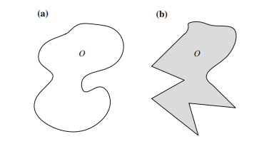
Condition (ii) implies that $\mathrm{L}(y, z)$ does not penetrate into the interior of $\mathcal{O}$, and $\mathrm{L}(y, z) \cap \partial \mathcal{O}$ may be nonempty. In the case where diffraction phenomenon occurs, we may replace $\mathrm{L}(y, z)$ in Definition $2.1$ by a smooth arc (in a given class) connecting the points $y$ and $z$. Figure $2.1$ shows the visible and invisible sets of a point $z$ for observing a plane curve and a compact connected set in $\mathbb{R}^{2}$ indicated by solid and dashed curves respectively. Note that the boundary of the object in Fig. 2.1b has a flat portion. Thus, for the indicated observation point $z$ and observed point $y, \mathrm{~L}(y, z) \cap \partial \mathcal{O}$ is nonempty. The visible and invisible sets of an observation point for an opaque solid object in $\mathbb{R}^{3}$ are illustrated by Fig. 2.4.
Remark 2.1 When a point-observer $z$ has finite viewing aperture such as a camera, we may define the visible set of the point-observer $z$ as
$$
\mathcal{V}(z)=\left{y \in\left(\mathcal{C}{z} \cap \partial O\right): \lambda z+(1-\lambda) y \notin O \text { for all } \lambda \in\right] 0,1[}, $$ where $\mathcal{C}{z}$ is the cone of visibility associated with the point-observer $z$ at its vertex, and has a finite viewing-aperture angle as illustrated in Fig. 2.5. In the case of a camera, its visible set may be enlarged by rotating the camera about the vertex of its viewingaperture cone. This approach may be useful when the object under observation does not change its shape significantly during the rotation period. Throughout this book,Remark $2.2$ In Definition $2.1$, visibility is defined in terms of line-of-sight observations. In practical situations, observations may be accomplished using more complex devices. For example, the observation of an object $\mathcal{O}$ may be made using a reflective surface $R_{f}$ as illustrated in Fig. 2.6. Here, a point $y \in \partial \mathcal{O}$ is visible from a point-observer $z \in \overline{\mathcal{O}^{c}}$, if there exists a ray composed of incident and reflected rays connecting $z$ and $y$. The direction of the reflected ray is determined by the usual Law of Reflection in optics (i.e. angle of incidence equals the angle of reflection). In this work, we only consider line-of-sight observations.
robotics代写|寻路算法代写Path Planning Algorithms|Observation of Complex Objects
So far, we have considered only the observation of an object consisting of a single connected compact set in the world space $\mathcal{W}$. In more general situations, the object $\mathcal{O}$ under observation may correspond to a collection of disjoint compact subsets $\mathcal{O}{i}, i \in \mathcal{I}$ of $\mathcal{W}$, where $\mathcal{I}$ is a finite or countably infinite index set. The observations of $\mathcal{O}$ are made from points $z \in \mathcal{P} \subset \mathcal{W}$ such that $\mathcal{P} \cap \mathcal{O}$ is empty. In the trivial case where the observation of any object $\mathcal{O}{i}$ can be made from a given observation point $z \in \mathcal{P}$ without considering the remaining subsets $\mathcal{O}{j}, j \in \mathcal{I}-{i}$, then the visible set $\mathcal{V}(z)$ is simply $\bigcup{i \in \mathcal{I}} \mathcal{V}{i}(z)$, where $\mathcal{V}{i}(z) \subset \partial \mathcal{O}{i}$ denotes the visible set of $z$ with respect to $\mathcal{O}{i}$. To illustrate various possible situations involving objects with multiple disjoint subsets, consider a simple example where the object $\mathcal{O} \subset \mathbb{R}^{2}$ consists of two circular disks $D_{i}, i=1,2$ with different radii $r_{1}$ and $r_{2}$ as shown in Fig. 2.23. First, consider the observation point $z^{(1)}$ located between the two disks. Evidently, both $D_{1}$ and $D_{2}$ are partially visible from $z^{(1)}$. From the observation point $z^{(2)}$ (resp. $z^{(3)}$ ), only $D_{1}$ (resp. $D_{2}$ ) is partially visible (as in solar eclipse, where the observation point $z$ is identified with the sun). From the observation $z^{(4)}$, both $D_{1}$ and $D_{2}$ are partially visible. However, only one point in $D_{1}$ is visible from $z^{(4)}$. Finally, both $D_{1}$ and $D_{2}$ are partially visible from the observation point $z^{(5)}$. Moreover, $\mathcal{V}\left(z^{(5)}\right)$, the visible set of $z^{(5)}$ is simply $\mathcal{V}{1}\left(z^{(5)}\right) \cup \mathcal{V}{2}\left(z^{(5)}\right)$, where $\mathcal{V}{i}\left(z^{(5)}\right)$ denotes the visible set of $z^{(5)}$ with respect to $D{i}$, which can be determined independently. This simple example shows
that the structure of the visible sets for objects with multiple disjoint subsets may be very complex, and their determination may be a computationally intensive task.
The following is an example of an object in $\mathcal{W}=\mathbb{R}^{3}$ : composed of an countably infinite number of disjoint compact subsets:
Example $2.4$ Let the object under observation be $\mathcal{O}=\cup_{i \in \mathcal{I}} \mathcal{O}{i}$, where $\mathcal{I}=$ ${1,2, \ldots}$, and $\mathcal{O}{i}$ is a circle with radius $r_{i}$, centered at $\left(x_{1}, x_{2}, x_{3}\right)=\left(0,0, x_{3 i}\right)$ :
$$
\mathcal{O}{i}=\left{x=\left(x{1}, x_{2}, x_{3}\right) \in \mathbb{R}^{3}: x_{1}^{2}+x_{2}^{2}=r_{i}^{2}, x_{3}=x_{3 i}=1 / i^{2}\right}, \quad i=1,2, \ldots
$$
such that $\mathcal{O}{i} \cap \mathcal{O}{j}$ is empty for all $i, j \in \mathcal{I}, i \neq j$. The observation platform $\mathcal{P}$ may correspond to a nonempty compact subset of $\mathcal{O}^{c}$, the complement of $\mathcal{O}$ relative to $\mathcal{W}$. The visible set of an observation point $z \in \mathcal{P}$ is given by
$$
\mathcal{V}(z)=\bigcup_{i \in \mathcal{I}} \mathcal{V}{i}(z) $$ where $\mathcal{V}{i}(z)$ is the set of all boundary points of $\mathcal{O}{i}$ that is visible from $z$. The object $\mathcal{O}$ is said to be totally visible from $z$ if $\mathcal{V}(z)=\bigcup{i \in \mathcal{I}} \partial \mathcal{O}{i}$, i.e. the boundary points of every $\mathcal{O}{i}$ are visible from $z$. Evidently, there does not exist an observation point $z \in \mathcal{O}^{c}$ from which $\mathcal{O}$ is totally visible.
In planetary explorations using mobile robots, one may encounter cavities and tunnel-like structures on the planet surface. Here, the object $\mathcal{O}$ under observation is the surface inside these structures. To describe $\mathcal{O}$ mathematically, consider the simple idealized case in the world space $\mathcal{W}=\mathbb{R}^{2}$ where $\mathcal{O}$ is the union of the graphs of two real-valued $C_{1}$ functions $f_{i}=f_{i}(x), i=1,2$ defined on the interval $[a, b]$ as shown in Fig. 2.24. In Fig. 2.24a, $G_{f_{1}}$ and $G_{f_{2}}$ intersect at $x=b$ where $f_{1}(b)=f_{2}(b)$.
robotics代写|寻路算法代写Path Planning Algorithms|Concluding Remarks
In this chapter, we have introduced various notions of visibility associated with line-of-sight observation of an object from a point-observer. These notions are also applicable to target interception by replacing the point-observer with a point source, and the object under observation with a target (e.g. a laser source emitting a beam toward the target). We may rename the “visible set of a point observer”as the “impact set of the point source”. Thus, total visibility of an object from a point-observer corresponds to total impact of the target boundary by a point source, i.e. each point of the target boundary can be impacted by at least one straight beam emitted from the source. In practical applications, it may be of interest to expose a particular part of the target surface to the source. This task can be accomplished only when that particular part lies in the impact set of the source.
Exercises
Ex.2.1. Let $\mathcal{W}=\mathbb{R}^{2}$. For each of the objects $\mathcal{O} \subset \mathcal{W}$ whose boundaries are composed of circular arcs and straightline segments (see Fig.2.26), determine the smallest number and locations of point-observers in $\mathcal{O}^{c}$ for total visibility of $\mathcal{O}$.
Ex.2.2. Let $\mathcal{W}=\mathbb{R}^{2}$. The object $\mathcal{O}$ under observation is formed by the union of two circular disks with different radii $r_{1}, r_{2}>0$.
(i) Find the visible sets of various observation points $z \in \mathcal{O}^{c}$ for each of the following cases:
(a) two disks are tangent to each other;
(b) two disks are disjoint with their centers separated by a finite distance $r_{1}+$ $r_{2}+d, d>0$.
寻路算法代写
robotics代写|寻路算法代写Path Planning Algorithms|Notions of Visibility
首先,我们考虑对象这具有如情况 (i) 和 (ii) 中所述的时不变形状。我们引入了一个点的可见性的概念是在∂这从观察点和,假设世界空间中没有其他物体或障碍物在. 除非另有说明,否则假设被观察的物体是不透明的,并且观察点和∈这C¯. 观察点的可见性基于观察点的视线和.
定义 2.1 一个点是∈∂这从观察点可见和∈这¯, 如果我)大号(是,和)⊂在, 和 (ii)大号(是,和)∩整数(这)=φ(空集),其中大号(是,和)是连接点的线段是和和由描述\left{x \in \mathbb{R}^{3}: x=\lambda y+(1-\lambda) z, 0<\right.$ $\lambda<1}\left{x \in \mathbb{R}^{3}: x=\lambda y+(1-\lambda) z, 0<\right.$ $\lambda<1}, 和 int(这)表示内部这. 套装在(和)所有点是∈∂这从某个点可见和∈这C¯称为可见集和. 的补充在(和)关系到∂这称为不可见集和.
条件 (ii) 意味着大号(是,和)不会渗透到内部这, 和大号(是,和)∩∂这可能是非空的。在出现衍射现象的情况下,我们可以更换大号(是,和)在定义2.1通过连接点的平滑弧(在给定类中)是和和. 数字2.1显示点的可见和不可见集和用于观察平面曲线和紧连通集R2分别用实线和虚线表示。请注意,图 2.1b 中对象的边界具有平坦部分。因此,对于指定的观察点和和观察点是, 大号(是,和)∩∂这是非空的。不透明固体物体的可见和不可见观测点集R3如图 2.4 所示。
备注 2.1 当点观察者和具有有限的观察孔径,例如相机,我们可以定义点观察者的可见集和作为
\mathcal{V}(z)=\left{y \in\left(\mathcal{C}{z} \cap \partial O\right): \lambda z+(1-\lambda) y \notin O \text { 对于所有 } \lambda\in\right] 0.1[},\mathcal{V}(z)=\left{y \in\left(\mathcal{C}{z} \cap \partial O\right): \lambda z+(1-\lambda) y \notin O \text { 对于所有 } \lambda\in\right] 0.1[},在哪里C和是与点观察者相关的可见锥和如图 2.5 所示,在其顶点处具有有限的视角。在相机的情况下,可以通过围绕其视孔锥的顶点旋转相机来扩大其可见集。当被观察的物体在旋转期间没有显着改变其形状时,这种方法可能很有用。在本书中,备注2.2在定义中2.1,可见性是根据视线观察定义的。在实际情况下,可以使用更复杂的设备完成观察。例如,观察一个物体这可以使用反射面制成RF如图 2.6 所示。在这里,一个点是∈∂这从点观察者可见和∈这C¯, 如果存在一条由入射光线和反射光线组成的光线和和是. 反射光线的方向由光学中通常的反射定律确定(即入射角等于反射角)。在这项工作中,我们只考虑视线观察。
robotics代写|寻路算法代写Path Planning Algorithms|Observation of Complex Objects
到目前为止,我们只考虑了对世界空间中由单个连通紧集组成的对象的观察在. 在更一般的情况下,对象这在观察下可能对应于一组不相交的紧凑子集这一世,一世∈一世的在, 在哪里一世是一个有限或可数无限的索引集。的观察这由点组成和∈磷⊂在这样磷∩这是空的。在观察任何物体的微不足道的情况下这一世可以从给定的观察点进行和∈磷不考虑其余子集这j,j∈一世−一世,那么可见集在(和)简直就是⋃一世∈一世在一世(和), 在哪里在一世(和)⊂∂这一世表示可见集和关于这一世. 为了说明涉及具有多个不相交子集的对象的各种可能情况,考虑一个简单的示例,其中对象这⊂R2由两个圆盘组成D一世,一世=1,2具有不同的半径r1和r2如图 2.23 所示。一、考虑观察点和(1)位于两个磁盘之间。显然,两者D1和D2部分可见和(1). 从观察点和(2)(分别。和(3)), 只要D1(分别。D2) 是部分可见的(如在日食中,观察点在和被识别为太阳)。从观察和(4), 两个都D1和D2部分可见。然而,只有一点D1从可见和(4). 最后,两者D1和D2从观察点部分可见和(5). 而且,在(和(5)),可见集和(5)简直就是在1(和(5))∪在2(和(5)), 在哪里在一世(和(5))表示可见集和(5)关于D一世,可以独立确定。这个简单的例子显示
具有多个不相交子集的对象的可见集的结构可能非常复杂,并且它们的确定可能是一项计算密集型任务。
下面是一个对象的例子在=R3:由无数个不相交的紧凑子集组成:
例子2.4设观察对象为这=∪一世∈一世这一世, 在哪里一世= 1,2,…, 和这一世是一个有半径的圆r一世, 以(X1,X2,X3)=(0,0,X3一世) :
\mathcal{O}{i}=\left{x=\left(x{1}, x_{2}, x_{3}\right) \in \mathbb{R}^{3}: x_{1} ^{2}+x_{2}^{2}=r_{i}^{2}, x_{3}=x_{3 i}=1 / i^{2}\right}, \quad i=1 ,2, \ldots\mathcal{O}{i}=\left{x=\left(x{1}, x_{2}, x_{3}\right) \in \mathbb{R}^{3}: x_{1} ^{2}+x_{2}^{2}=r_{i}^{2}, x_{3}=x_{3 i}=1 / i^{2}\right}, \quad i=1 ,2, \ldots
这样这一世∩这j对所有人都是空的一世,j∈一世,一世≠j. 观景台磷可能对应于一个非空紧凑子集这C, 的补码这关系到在. 观察点的可见集和∈磷是(谁)给的
在(和)=⋃一世∈一世在一世(和)在哪里在一世(和)是所有边界点的集合这一世这是可见的和. 物体这据说是完全可见的和如果在(和)=⋃一世∈一世∂这一世,即每个的边界点这一世可以从和. 显然,不存在观察点和∈这C从中这是完全可见的。
在使用移动机器人进行行星探索时,人们可能会在行星表面遇到空洞和隧道状结构。在这里,对象这正在观察的是这些结构内部的表面。来描述这在数学上,考虑世界空间中的简单理想化情况在=R2在哪里这是两个实值图的并集C1职能F一世=F一世(X),一世=1,2在区间上定义[一种,b]如图 2.24 所示。在图 2.24a 中,GF1和GF2相交于X=b在哪里F1(b)=F2(b).
robotics代写|寻路算法代写Path Planning Algorithms|Concluding Remarks
在本章中,我们介绍了与从点观察者对物体的视线观察相关的各种可见性概念。这些概念也适用于通过将点观察器替换为点源来进行目标拦截,以及将被观察对象替换为目标(例如,向目标发射光束的激光源)。我们可以将“点观察者的可见集”重命名为“点源的影响集”。因此,来自点观察者的对象的总可见性对应于点源对目标边界的总影响,即目标边界的每个点都可以受到从源发射的至少一个直光束的影响。在实际应用中,将目标表面的特定部分暴露给源可能是有意义的。
练习
Ex.2.1。让在=R2. 对于每个对象这⊂在其边界由圆弧和直线段组成(见图 2.26),确定点观测器的最小数量和位置这C总能见度这.
例 2.2。让在=R2. 物体这观察下是由两个不同半径的圆盘结合而成r1,r2>0.
(i) 找到各个观察点的可见集和∈这C对于以下每种情况:
(a) 两个圆盘彼此相切;
(b) 两个圆盘不相交,它们的中心相隔有限距离r1+ r2+d,d>0.

统计代写请认准statistics-lab™. statistics-lab™为您的留学生涯保驾护航。
金融工程代写
金融工程是使用数学技术来解决金融问题。金融工程使用计算机科学、统计学、经济学和应用数学领域的工具和知识来解决当前的金融问题,以及设计新的和创新的金融产品。
非参数统计代写
非参数统计指的是一种统计方法,其中不假设数据来自于由少数参数决定的规定模型;这种模型的例子包括正态分布模型和线性回归模型。
广义线性模型代考
广义线性模型(GLM)归属统计学领域,是一种应用灵活的线性回归模型。该模型允许因变量的偏差分布有除了正态分布之外的其它分布。
术语 广义线性模型(GLM)通常是指给定连续和/或分类预测因素的连续响应变量的常规线性回归模型。它包括多元线性回归,以及方差分析和方差分析(仅含固定效应)。
有限元方法代写
有限元方法(FEM)是一种流行的方法,用于数值解决工程和数学建模中出现的微分方程。典型的问题领域包括结构分析、传热、流体流动、质量运输和电磁势等传统领域。
有限元是一种通用的数值方法,用于解决两个或三个空间变量的偏微分方程(即一些边界值问题)。为了解决一个问题,有限元将一个大系统细分为更小、更简单的部分,称为有限元。这是通过在空间维度上的特定空间离散化来实现的,它是通过构建对象的网格来实现的:用于求解的数值域,它有有限数量的点。边界值问题的有限元方法表述最终导致一个代数方程组。该方法在域上对未知函数进行逼近。[1] 然后将模拟这些有限元的简单方程组合成一个更大的方程系统,以模拟整个问题。然后,有限元通过变化微积分使相关的误差函数最小化来逼近一个解决方案。
tatistics-lab作为专业的留学生服务机构,多年来已为美国、英国、加拿大、澳洲等留学热门地的学生提供专业的学术服务,包括但不限于Essay代写,Assignment代写,Dissertation代写,Report代写,小组作业代写,Proposal代写,Paper代写,Presentation代写,计算机作业代写,论文修改和润色,网课代做,exam代考等等。写作范围涵盖高中,本科,研究生等海外留学全阶段,辐射金融,经济学,会计学,审计学,管理学等全球99%专业科目。写作团队既有专业英语母语作者,也有海外名校硕博留学生,每位写作老师都拥有过硬的语言能力,专业的学科背景和学术写作经验。我们承诺100%原创,100%专业,100%准时,100%满意。
随机分析代写
随机微积分是数学的一个分支,对随机过程进行操作。它允许为随机过程的积分定义一个关于随机过程的一致的积分理论。这个领域是由日本数学家伊藤清在第二次世界大战期间创建并开始的。
时间序列分析代写
随机过程,是依赖于参数的一组随机变量的全体,参数通常是时间。 随机变量是随机现象的数量表现,其时间序列是一组按照时间发生先后顺序进行排列的数据点序列。通常一组时间序列的时间间隔为一恒定值(如1秒,5分钟,12小时,7天,1年),因此时间序列可以作为离散时间数据进行分析处理。研究时间序列数据的意义在于现实中,往往需要研究某个事物其随时间发展变化的规律。这就需要通过研究该事物过去发展的历史记录,以得到其自身发展的规律。
回归分析代写
多元回归分析渐进(Multiple Regression Analysis Asymptotics)属于计量经济学领域,主要是一种数学上的统计分析方法,可以分析复杂情况下各影响因素的数学关系,在自然科学、社会和经济学等多个领域内应用广泛。
MATLAB代写
MATLAB 是一种用于技术计算的高性能语言。它将计算、可视化和编程集成在一个易于使用的环境中,其中问题和解决方案以熟悉的数学符号表示。典型用途包括:数学和计算算法开发建模、仿真和原型制作数据分析、探索和可视化科学和工程图形应用程序开发,包括图形用户界面构建MATLAB 是一个交互式系统,其基本数据元素是一个不需要维度的数组。这使您可以解决许多技术计算问题,尤其是那些具有矩阵和向量公式的问题,而只需用 C 或 Fortran 等标量非交互式语言编写程序所需的时间的一小部分。MATLAB 名称代表矩阵实验室。MATLAB 最初的编写目的是提供对由 LINPACK 和 EISPACK 项目开发的矩阵软件的轻松访问,这两个项目共同代表了矩阵计算软件的最新技术。MATLAB 经过多年的发展,得到了许多用户的投入。在大学环境中,它是数学、工程和科学入门和高级课程的标准教学工具。在工业领域,MATLAB 是高效研究、开发和分析的首选工具。MATLAB 具有一系列称为工具箱的特定于应用程序的解决方案。对于大多数 MATLAB 用户来说非常重要,工具箱允许您学习和应用专业技术。工具箱是 MATLAB 函数(M 文件)的综合集合,可扩展 MATLAB 环境以解决特定类别的问题。可用工具箱的领域包括信号处理、控制系统、神经网络、模糊逻辑、小波、仿真等。