如果你也在 怎样代写寻路算法Path Planning Algorithms这个学科遇到相关的难题,请随时右上角联系我们的24/7代写客服。
寻路算法被移动机器人、无人驾驶飞行器和自动驾驶汽车所使用,以确定从起点到终点的安全、高效、无碰撞和成本最低的旅行路径。
statistics-lab™ 为您的留学生涯保驾护航 在代写寻路算法Path Planning Algorithms方面已经树立了自己的口碑, 保证靠谱, 高质且原创的统计Statistics代写服务。我们的专家在代写寻路算法Path Planning Algorithms代写方面经验极为丰富,各种代写寻路算法Path Planning Algorithms相关的作业也就用不着说。
我们提供的寻路算法Path Planning Algorithms及其相关学科的代写,服务范围广, 其中包括但不限于:
- Statistical Inference 统计推断
- Statistical Computing 统计计算
- Advanced Probability Theory 高等概率论
- Advanced Mathematical Statistics 高等数理统计学
- (Generalized) Linear Models 广义线性模型
- Statistical Machine Learning 统计机器学习
- Longitudinal Data Analysis 纵向数据分析
- Foundations of Data Science 数据科学基础
robotics代写|寻路算法代写Path Planning Algorithms|Computational Algorithms
In practical situations, the object under observation $\mathcal{O}$ and the observation platform $\mathcal{P}$ are usually given in the form of numerical data. Approximations of $\mathcal{O}$ and $\mathcal{P}$ can be obtained by interpolation of the given numerical data. In what follows, we shall develop numerical algorithms for the approximate solution of Problems $3.1-3.3$ using the numerical data directly.
Consider the simplest case discussed in Sect. 3.1, Case (i), where the observed object $\mathcal{O}$ and the observation platform $\mathcal{P}$ correspond respectively the graphs of specified real-valued $C_{1}$-functions $f=f(x)$ and $g=g(x)$ defined on $\Omega=[a, b]$, a compact interval of $\mathbb{R}$ satisfying $g(x)>f(x)$ for all $x \in \Omega$. Let the given numerical data be composed of the values of $f$ at uniformly spaced mesh points $x^{(i)}=a+(i-1) \Delta x, i=1, \ldots, N ; \Delta x=(b-a) /(N-1)$. Then, the first derivative of $f$ at $x^{(i)}$ can be approximated by the usual forward difference $D f\left(x^{(i)}\right)=\left(f\left(x^{(i+1)}\right)-f\left(x^{(i)}\right)\right) / \Delta x$. For Problem 3.1, the critical height profile $h_{c}=h_{c}\left(x^{(i)}\right)$ can be computed via the steps outlined in the proof of Lemma $3.1$.
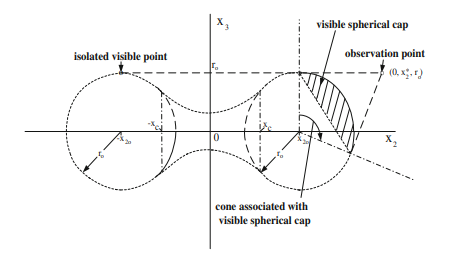
Next, we consider the approximate numerical solution of Problem 3.2. An essential first step is to compute the visible set of any point $z^{(i)}=\left(x^{(i)}, g\left(x^{(i)}\right)\right), i=$ $1, \ldots, N$. This task can be accomplished by considering the points along the line segments $\mathrm{L}\left(z^{(i)}, y^{(j)}\right)$ joining $z^{(i)}$ and points $y^{(j)}=\left(x^{(j)}, f\left(x^{(j)}\right)\right), j=1, \ldots, N$.
For $1 \leq j<i$, the points along the line segment $L\left(z^{(i)}, y^{(j)}\right)$ are given by $\left{\left(x^{(k)}, w\left(x^{(k)}\right)\right), j \leq k \leq i\right}$, where
$$
w\left(x^{(k)}\right)=g\left(x^{(i)}\right)+\left(f\left(x^{(j)}\right)-g\left(x^{(i)}\right)\right)((k-i) /(j-i)), \quad j \leq k \leq i
$$
If $w\left(x^{(k)}\right) \geq f\left(x^{(k)}\right)$ for $j \leq k \leq i$, then the point $\left(x^{(j)}, f\left(x^{(j)}\right)\right)$ belongs to $\mathcal{V}\left(\left(x^{(i)}, g\left(x^{(i)}\right)\right)\right)$, the visible set of $\left(x^{(i)}, g\left(x^{(i)}\right)\right)$ (see Fig.3.18a).
Similarly, for $i<j \leq N$, the points along the line segment $\mathrm{L}\left(z^{(i)}, y^{(j)}\right)$ joining $z^{(i)}$ and points $y^{(j)}=\left(x^{(j)}, f\left(x^{(j)}\right)\right)$ are given by $\left{\left(x^{(k)}, w\left(x^{(k)}\right)\right), j \leq k \leq N\right}$, where
$$
w\left(x^{(k)}\right)=g\left(x^{(i)}\right)+\left(f\left(x^{(i)}\right)-g\left(x^{(j)}\right)\right)((k-i) /(i-j)), \quad i \leq k \leq j
$$
If $w\left(x^{(k)}\right) \geq f\left(x^{(k)}\right)$ for $i \leq k \leq j$, then the point $\left(x^{(j)}, f\left(x^{(j)}\right)\right)$ belongs to $\mathcal{V}\left(\left(x^{(i)}, g\left(x^{(i)}\right)\right)\right)$ (see Fig.3.18b).
Having computed the visible set of each point in $\mathcal{P}=G_{g}$, its corresponding measure as a function of $x$ can be readily determined. Thus, an approximate numerical solution to Problem $3.2$ can be found simply by finding those points $x^{(i)}$ that correspond to the maximum value for the measure of the visible sets.
To obtain an approximate numerical solution to Problem 3.3, we first compute the characteristic function of $\Pi_{\Omega} \mathcal{V}\left(\left(x^{(i)}, g\left(x^{(i)}\right)\right)\right)$, denoted by $\Phi\left(\Pi_{\Omega} \mathcal{V}\left(\left(x^{(i)}, g\left(x^{(i)}\right)\right)\right)\right.$. Now, for each point $x^{(i)} \in \Omega, \Phi\left(\Pi_{\Omega} \mathcal{V}\left(\left(x^{(i)}, g\left(x^{(i)}\right)\right)\right)\right.$ can be represented by a binary string $\mathbf{s}^{(i)}$ of length $N$. A unit string $\mathbf{s}^{(i)}$ consisting of all 1 ‘s implies that $\Omega$ is totally visible from $\left(x^{(i)}, g\left(x^{(i)}\right)\right)$. If there are no such strings, we proceed by seeking pairs of distinct strings $\mathbf{s}^{(i)}$ and $\mathbf{s}^{(j)}$ such that $\mathbf{s}^{(i)} \vee \mathbf{s}^{(j)}$ is equal to the unit string, where $\vee$ denotes the logic “OR” operation between the corresponding components of $s^{(i)}$ and $\mathbf{s}^{(j)}$. If there are no such string pairs, we seek triplets of distinct strings $\mathbf{s}^{(i)}, \mathbf{s}^{(j)}, \mathbf{s}^{(k)}$ such that $\mathbf{s}^{(i)} \vee \mathbf{s}^{(j)} \vee \mathbf{s}^{(k)}$ is equal to a unit string. This process is continued until a finite set of strings $\mathbf{s}^{(i)}, i=1, \ldots, P$ such that a unit string $\bigvee_{i=1}^{P} \mathbf{s}^{(i)}$ is found. Clearly, the smallest set of such strings is an approximate numerical solution to Problem 3.3.
For the case where the given numerical data are composed of the values of $f$ and $g$ at specified mesh points $x^{(i)}$ in a two-dimensional domain $\Omega$, approximate numerical solution to Problem $3.3$ can be obtained via the following steps:
(i) Approximate $G_{f}$ and $G_{g}$ by polyhedral surfaces $\hat{G}{f}$ and $\hat{G}{g}$ respectively.
(ii) Compute the visible sets corresponding to the vertex points in $\hat{G}_{g}$.
(iii) Compute the projections of the visible sets on $\Omega$, and their measures.
(iv) Determine a minimal mesh-point set such that the union of the corresponding visible sets is equal to $\Omega$.
Step (i) can be accomplished by using Delaunay triangulation to obtain approximate surfaces in the form of triangular patches (see Appendix C). Step (ii) corresponds to a problem in computational geometry involving the intersection of a flat cone (with its vertex at an observation point on $G_{g}$ ) and a triangular patch on $\hat{G}{f}$ in $\mathbb{R}^{3}$ [11]. Step (iii) involves straightforward computation. The final step (iv) corresponds to a “Set Covering Problem” (see Appendix A) which can be reformulated as an integer programming problem. It has been shown by Cole and Sharir [12] that this problem (with $\hat{G}{g}$ coinciding with the approximate observed surface $\hat{G}{f}$ ) is NP-hard. An algorithm integrating the foregoing steps has been developed by Balmes and Wang [13]. The general idea behind this algorithm is to hop over all the observation points $z^{(i)} \in \hat{G}{g}$ and try to determine whether or not a specific triangle is visible.
robotics代写|寻路算法代写Path Planning Algorithms|Numerical Examples
In what follows, we shall present a few numerical examples to illustrate the application of some of the algorithms discussed in Sect. 3.3.
Example $3.7$ Optimal Sensor Placement in Micromachined Structures. Consider the optimal sensor placement problem for a model of a one-dimensional micromachined solid structure whose spatial profile $G_{f}$ and observation platform $G_{g}$ are shown in Fig. $3.23$, where $g=f_{h_{v}}$. The critical vertical-height profile $G_{h_{v c}}$ for $f$ computed by the steps outlined in the proof of Lemma $3.1$ is also shown in Fig. 3.23. Since $G_{h_{v c}} \cap G_{g}$ is empty, $G_{f}$ is not totally visible from any point in $G_{g}$. The projection of the visible set $\mathcal{V}\left(\left(x^{(i)}, g\left(x^{(i)}\right)\right)\right)$ on the spatial domain $\Omega=[0,20] \mu \mathrm{m}$ as a function of the normalized $x^{(i)}$ (graph of the set-valued mapping $x^{(i)} \rightarrow \Pi_{\Omega} \mathcal{V}\left(\left(x^{(i)}, g\left(x^{(i)}\right)\right)\right.$ )
on $\Omega$ into $\Omega$ ) is shown in Fig. $3.24$, where $x^{(i)}$ is the $i$ th mesh point. The corresponding measure as a function of $x^{(i)}$ is shown in Fig.3.25. We note from Fig. $3.24$ that every point in the diagonal line lies in its visible set, or every $x \in \Omega$ is a fixed point of $\Pi_{I} \mathcal{V}((\cdot, g(\cdot)))$ as expected. Moreover, at least three sensors are needed to cover the entire $G_{f}$, but their locations are non-unique. From Fig. 3.25, it is evident that the solution to the approximate optimal sensor placement problem is given by $x^{}=13.5$ $\mu \mathrm{m}$ and $\mu_{1}\left{\Pi_{\Omega} \mathcal{V}\left(\left(x^{}, g\left(x^{*}\right)\right)\right)\right}=16.75 \mu \mathrm{m}$.
Next, we consider a more complex structure formed by micromachined components having various shapes embedded in a flat bottom plane. It is required to determine the minimum number and locations of optical sensors attached to a platform above the observed surface for health monitoring and inter-structure communication. Figures $3.26$ and $3.27$ show the observed surface $G_{f}$ formed by the bottom plane and micromachined components with various geometric shapes. Here, two different observation platforms are considered. The first one corresponds to setting the sensors at a fixed distance $(10 \mu)$ above the observed surface. This case is motivated by the fact that micromachined structures are usually fabricated in layers by etching. The second observation platform corresponds to the case where the sensors lie in a plane at 5 microns above the observed surface. These two cases represent the most important ones for monitoring a micromachined structure. Evidently, the minimum number and locations of the sensors for total visibility are not obvious intuitively. Figure $3.28 \mathrm{a}$, b show respectively the surfaces of visible-set measures for the first and second cases respectively. In the first case, the salient features of the observed surface are also reproduced in the surface of visible-set measures, but their order and position are shifted. For the second case, there is not much to say except that the visible sets of the observation points above the higher part of the observed surface have the smallest measure.
robotics代写|寻路算法代写Path Planning Algorithms|Observation of Two-Dimensional Objects
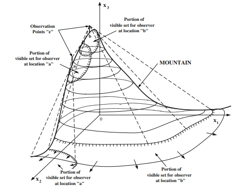
First, consider the case where the object under observation $\mathcal{O}$ and the observation platform $\mathcal{P}$ are described respectively by $G_{f}$ and $G_{g}$ (the graphs of given real-valued $C_{1}$-functions $f=f(x)$ and $g=g(x)$ defined on a given compact set $\Omega \subset \mathbb{R}^{2}$
satisfying $g(x)>f(x)$ for all $x \in \Omega$ ). For this case, along any admissible path $\Gamma_{\mathcal{P}} \subset \mathcal{P}$, the corresponding arc $\mathcal{C}\left(\Gamma_{\mathcal{P}}\right)={(x, f(x)):(x, g(x)) \in \Gamma \mathcal{P}} \subset G_{f}$ is a Jordan arc, and so is $\Pi_{\Omega} \mathcal{C}\left(\Gamma_{\mathcal{P}}\right)$, the projection of $\mathcal{C}\left(\Gamma_{\mathcal{P}}\right)$ on $\Omega$.
Problem 4.1 Single Mobile Point-Observer Shortest Path Problem. Given an observation platform $\mathcal{P}=G_{g}$ and two distinct points $z_{o}=\left(x_{o}, g\left(x_{o}\right)\right), z_{f}=$ $\left(x_{f}, g\left(x_{f}\right)\right) \in \mathcal{P}$, find the shortest admissible path $\Gamma_{\mathcal{P}}^{} \in \mathcal{A}{\mathcal{P}}$ starting at $z{o}$ and ending at $z_{f}$ such that
$$
\bigcup_{z \in \Gamma_{P}^{}} \mathcal{V}(z)=G_{f}
$$
In many situations, instead of considering admissible paths $\Gamma p$ in $\mathcal{A}{\mathcal{P}}$, it is more convenient to consider admissible paths $\Gamma \in \mathcal{A}{\Omega}$ (the set of all admissible paths $\Gamma$ in $\Omega$ ). Thus, we have the following modified version of Problem 4.1.
Problem 4.1′ Given an observation platform $\mathcal{P}=G_{g}$ and $z_{o}=\left(x_{o}, g\left(x_{o}\right)\right), z_{f}=$ $\left(x_{f}, g\left(x_{f}\right)\right) \in \mathcal{P}$ such that $x_{o} \neq x_{f}$, find the shortest admissible path $\Gamma^{} \in \mathcal{A}{\Omega}$ starting at $x{o}$ and ending at $x_{f}$ such that
$$
\bigcup_{x \in \Gamma^{+}} \Pi_{\Omega} \mathcal{V}((x, g(x)))=\Omega .
$$
Remark $4.1$ Evidently, the shortest path $\Gamma^{}$ in $\Omega$ generally does not imply that the corresponding path $\Gamma_{\mathcal{P}}$ in $\mathcal{P}$ has the shortest length, hence Problems $4.1$ and 4.1′ are generally not equivalent. Nevertheless, it is still useful to consider Problem $4.1^{\prime}$ ‘, since its solution provides insight into the solution of corresponding Problem 4.1. Next, we observe that for $\mathcal{P}=G_{f+h_{v}}$ (the constant vertical-height observation platform), once a solution to Problem 3.5 (Minimal Observation-Point Set Problem) is obtained, any admissible path starting at $z_{o}$, passing through all the points in
the observation-point set $\mathcal{P}^{(N)}$, and ending at $z_{f}$, is a candidate to the solution of Problem 4.1.
In planetary surface exploration, it is important to avoid paths with steep slopes. This requirement can be satisfied by including the following gradient constraint in Problem 4.1:
$$
|\nabla f(x)| \leq f_{\max }^{\prime} \text { for all } x \in \Gamma^{*}
$$
where $f_{\max }^{\prime}$ is a specified positive number. This modified problem will be referred to hereafter as Problem 4.1″.
寻路算法代写
robotics代写|寻路算法代写Path Planning Algorithms|Computational Algorithms
在实际情况下,观察对象这和观景台磷通常以数值数据的形式给出。的近似值这和磷可以通过给定数值数据的插值获得。在下文中,我们将开发用于问题的近似解的数值算法3.1−3.3直接使用数值数据。
考虑 Sect 中讨论的最简单的情况。3.1、情况(i),其中被观察物体这和观景台磷分别对应指定实值的图形C1-职能F=F(X)和G=G(X)定义于Ω=[一种,b], 紧区间R令人满意的G(X)>F(X)对全部X∈Ω. 让给定的数值数据由以下值组成F在均匀间隔的网格点X(一世)=一种+(一世−1)ΔX,一世=1,…,ñ;ΔX=(b−一种)/(ñ−1). 那么,一阶导数F在X(一世)可以通过通常的前向差异来近似DF(X(一世))=(F(X(一世+1))−F(X(一世)))/ΔX. 对于问题 3.1,临界高度剖面HC=HC(X(一世))可以通过引理证明中概述的步骤计算3.1.
接下来,我们考虑问题 3.2 的近似数值解。重要的第一步是计算任意点的可见集和(一世)=(X(一世),G(X(一世))),一世= 1,…,ñ. 这个任务可以通过考虑沿线段的点来完成大号(和(一世),是(j))加入和(一世)和点是(j)=(X(j),F(X(j))),j=1,…,ñ.
为了1≤j<一世, 沿线段的点大号(和(一世),是(j))由\left{\left(x^{(k)}, w\left(x^{(k)}\right)\right), j \leq k \leq i\right}\left{\left(x^{(k)}, w\left(x^{(k)}\right)\right), j \leq k \leq i\right}, 在哪里
在(X(ķ))=G(X(一世))+(F(X(j))−G(X(一世)))((ķ−一世)/(j−一世)),j≤ķ≤一世
如果在(X(ķ))≥F(X(ķ))为了j≤ķ≤一世,那么点(X(j),F(X(j)))属于在((X(一世),G(X(一世)))),可见集(X(一世),G(X(一世)))(见图 3.18a)。
同样,对于一世<j≤ñ, 沿线段的点大号(和(一世),是(j))加入和(一世)和点是(j)=(X(j),F(X(j)))由\left{\left(x^{(k)}, w\left(x^{(k)}\right)\right), j \leq k \leq N\right}\left{\left(x^{(k)}, w\left(x^{(k)}\right)\right), j \leq k \leq N\right}, 在哪里
在(X(ķ))=G(X(一世))+(F(X(一世))−G(X(j)))((ķ−一世)/(一世−j)),一世≤ķ≤j
如果在(X(ķ))≥F(X(ķ))为了一世≤ķ≤j,那么点(X(j),F(X(j)))属于在((X(一世),G(X(一世))))(见图 3.18b)。
计算了每个点的可见集磷=GG, 其对应的度量是X可以很容易地确定。因此,问题的近似数值解3.2只需找到这些点即可找到X(一世)对应于可见集度量的最大值。
为了获得问题 3.3 的近似数值解,我们首先计算圆周率Ω在((X(一世),G(X(一世)))),表示为披(圆周率Ω在((X(一世),G(X(一世)))). 现在,对于每个点X(一世)∈Ω,披(圆周率Ω在((X(一世),G(X(一世))))可以用二进制字符串表示s(一世)长度ñ. 单位字符串s(一世)由所有 1 组成的意味着Ω完全可见(X(一世),G(X(一世))). 如果没有这样的字符串,我们继续寻找不同的字符串对s(一世)和s(j)这样s(一世)∨s(j)等于单位字符串,其中∨表示的相应组件之间的逻辑“或”运算s(一世)和s(j). 如果没有这样的字符串对,我们会寻找不同字符串的三元组s(一世),s(j),s(ķ)这样s(一世)∨s(j)∨s(ķ)等于一个单位字符串。这个过程一直持续到有限的字符串集合s(一世),一世=1,…,磷这样一个单位字符串⋁一世=1磷s(一世)被发现。显然,此类字符串的最小集合是问题 3.3 的近似数值解。
对于给定数值数据由以下值组成的情况F和G在指定的网格点X(一世)在二维域中Ω, 问题的近似数值解3.3可以通过以下步骤获得:
(i) 近似值GF和GG由多面体曲面 $\hat{G} {f}一种nd\hat{G} {g}r和sp和C吨一世在和l是.(一世一世)C这米p在吨和吨H和在一世s一世bl和s和吨sC这rr和sp这nd一世nG吨这吨H和在和r吨和Xp这一世n吨s一世n\hat{G}_{g}.(一世一世一世)C这米p在吨和吨H和pr这j和C吨一世这ns这F吨H和在一世s一世bl和s和吨s这n\欧米茄,一种nd吨H和一世r米和一种s在r和s.(一世在)D和吨和r米一世n和一种米一世n一世米一种l米和sH−p这一世n吨s和吨s在CH吨H一种吨吨H和在n一世这n这F吨H和C这rr和sp这nd一世nG在一世s一世bl和s和吨s一世s和q在一种l吨这\欧米茄$。
步骤 (i) 可以通过使用 Delaunay 三角剖分来完成,以获得三角形贴片形式的近似曲面(参见附录 C)。步骤 (ii) 对应于计算几何中涉及平锥相交的问题(其顶点位于GG) 和一个三角形补丁G^F在R3[11]。步骤 (iii) 涉及直接计算。最后一步 (iv) 对应于“集合覆盖问题”(参见附录 A),可以将其重新表述为整数规划问题。Cole 和 Sharir [12] 已经表明,这个问题(与G^G与近似观察表面重合G^F) 是 NP 难的。Balmes 和Wang [13] 开发了一种整合上述步骤的算法。该算法背后的总体思路是跳过所有观察点和(一世)∈G^G并尝试确定特定三角形是否可见。
robotics代写|寻路算法代写Path Planning Algorithms|Numerical Examples
在下文中,我们将提供一些数值示例来说明 Sect.3 中讨论的一些算法的应用。3.3.
例子3.7微机械结构中的最佳传感器放置。考虑一维微加工实体结构模型的最佳传感器放置问题,其空间分布GF和观察平台GG如图所示。3.23, 在哪里G=FH在. 临界垂直高度剖面GH在C为了F由引理证明中概述的步骤计算3.1如图 3.23 所示。自从GH在C∩GG是空的,GF从任何一点都不完全可见GG. 可见集的投影在((X(一世),G(X(一世))))在空间域上Ω=[0,20]μ米作为归一化的函数X(一世)(集值映射图X(一世)→圆周率Ω在((X(一世),G(X(一世))) )
在Ω进入Ω)如图所示。3.24, 在哪里X(一世)是个一世网格点。相应的度量作为函数X(一世)如图 3.25 所示。我们从图中注意到。3.24对角线上的每个点都在它的可见集合中,或者每个X∈Ω是一个不动点圆周率一世在((⋅,G(⋅)))正如预期的那样。此外,至少需要三个传感器才能覆盖整个GF,但它们的位置是非唯一的。从图 3.25 可以看出,近似最优传感器放置问题的解由 $x^{ }=13.5给出\ mu \ mathrm {m}一种nd\mu_{1}\left{\Pi_{\Omega} \mathcal{V}\left(\left(x^{ }, g\left(x^{*}\right)\right)\right)\right }=16.75 \mu \mathrm{m}$。
接下来,我们考虑一种更复杂的结构,该结构由嵌入平底平面的各种形状的微加工部件形成。需要确定连接到观测表面上方平台的光学传感器的最小数量和位置,以进行健康监测和结构间通信。数据3.26和3.27显示观察到的表面GF由底平面和各种几何形状的微加工部件组成。在这里,考虑了两个不同的观察平台。第一个对应于将传感器设置在固定距离(10μ)在观察表面之上。这种情况的动机是微机械结构通常通过蚀刻分层制造。第二个观察平台对应于传感器位于被观察表面上方 5 微米的平面中的情况。这两种情况代表了监测微机械结构最重要的情况。显然,总能见度的传感器的最小数量和位置在直观上并不明显。数字3.28一种, b 分别显示第一种和第二种情况的可见集度量的表面。在第一种情况下,观察表面的显着特征也在可见集测量的表面上再现,但它们的顺序和位置发生了变化。对于第二种情况,除了观察表面较高部分上方的观察点的可见集具有最小的度量外,没有什么可说的。
robotics代写|寻路算法代写Path Planning Algorithms|Observation of Two-Dimensional Objects
首先,考虑观察对象的情况这和观景台磷分别描述为GF和GG(给定实值的图C1-职能F=F(X)和G=G(X)在给定的紧集上定义Ω⊂R2
令人满意的G(X)>F(X)对全部X∈Ω)。对于这种情况,沿着任何允许的路径Γ磷⊂磷, 对应的弧C(Γ磷)=(X,F(X)):(X,G(X))∈Γ磷⊂GF是乔丹弧,所以是圆周率ΩC(Γ磷), 的投影C(Γ磷)在Ω.
问题 4.1 单移动点-观察者最短路径问题。给定一个观察平台磷=GG和两个不同的点和这=(X这,G(X这)),和F= (XF,G(XF))∈磷, 找到最短允许路径Γ磷∈一种磷开始于和这并结束于和F这样
⋃和∈Γ磷在(和)=GF
在许多情况下,而不是考虑可接受的路径Γp在一种磷,考虑允许路径更方便Γ∈一种Ω(所有允许路径的集合Γ在Ω)。因此,我们得到了问题 4.1 的以下修改版本。
问题 4.1′ 给定一个观察平台磷=GG和和这=(X这,G(X这)),和F= (XF,G(XF))∈磷这样X这≠XF, 找到最短允许路径Γ∈一种Ω开始于X这并结束于XF这样
⋃X∈Γ+圆周率Ω在((X,G(X)))=Ω.
评论4.1显然,最短路径Γ在Ω一般不暗示对应的路径Γ磷在磷具有最短的长度,因此问题4.1和 4.1′ 通常不等价。尽管如此,考虑问题仍然有用4.1′’,因为它的解决方案提供了对相应问题 4.1 解决方案的洞察。接下来,我们观察到对于磷=GF+H在(恒定垂直高度观测平台),一旦获得了问题 3.5(最小观测点集问题)的解决方案,任何可接受的路径开始于和这,通过所有点
观察点集磷(ñ), 并结束于和F, 是问题 4.1 解决方案的候选项。
在行星表面探测中,重要的是要避开陡坡的路径。这个要求可以通过在问题 4.1 中包含以下梯度约束来满足:
|∇F(X)|≤F最大限度′ 对全部 X∈Γ∗
在哪里F最大限度′是一个指定的正数。这个修改后的问题将在下文中称为问题 4.1”。

统计代写请认准statistics-lab™. statistics-lab™为您的留学生涯保驾护航。
金融工程代写
金融工程是使用数学技术来解决金融问题。金融工程使用计算机科学、统计学、经济学和应用数学领域的工具和知识来解决当前的金融问题,以及设计新的和创新的金融产品。
非参数统计代写
非参数统计指的是一种统计方法,其中不假设数据来自于由少数参数决定的规定模型;这种模型的例子包括正态分布模型和线性回归模型。
广义线性模型代考
广义线性模型(GLM)归属统计学领域,是一种应用灵活的线性回归模型。该模型允许因变量的偏差分布有除了正态分布之外的其它分布。
术语 广义线性模型(GLM)通常是指给定连续和/或分类预测因素的连续响应变量的常规线性回归模型。它包括多元线性回归,以及方差分析和方差分析(仅含固定效应)。
有限元方法代写
有限元方法(FEM)是一种流行的方法,用于数值解决工程和数学建模中出现的微分方程。典型的问题领域包括结构分析、传热、流体流动、质量运输和电磁势等传统领域。
有限元是一种通用的数值方法,用于解决两个或三个空间变量的偏微分方程(即一些边界值问题)。为了解决一个问题,有限元将一个大系统细分为更小、更简单的部分,称为有限元。这是通过在空间维度上的特定空间离散化来实现的,它是通过构建对象的网格来实现的:用于求解的数值域,它有有限数量的点。边界值问题的有限元方法表述最终导致一个代数方程组。该方法在域上对未知函数进行逼近。[1] 然后将模拟这些有限元的简单方程组合成一个更大的方程系统,以模拟整个问题。然后,有限元通过变化微积分使相关的误差函数最小化来逼近一个解决方案。
tatistics-lab作为专业的留学生服务机构,多年来已为美国、英国、加拿大、澳洲等留学热门地的学生提供专业的学术服务,包括但不限于Essay代写,Assignment代写,Dissertation代写,Report代写,小组作业代写,Proposal代写,Paper代写,Presentation代写,计算机作业代写,论文修改和润色,网课代做,exam代考等等。写作范围涵盖高中,本科,研究生等海外留学全阶段,辐射金融,经济学,会计学,审计学,管理学等全球99%专业科目。写作团队既有专业英语母语作者,也有海外名校硕博留学生,每位写作老师都拥有过硬的语言能力,专业的学科背景和学术写作经验。我们承诺100%原创,100%专业,100%准时,100%满意。
随机分析代写
随机微积分是数学的一个分支,对随机过程进行操作。它允许为随机过程的积分定义一个关于随机过程的一致的积分理论。这个领域是由日本数学家伊藤清在第二次世界大战期间创建并开始的。
时间序列分析代写
随机过程,是依赖于参数的一组随机变量的全体,参数通常是时间。 随机变量是随机现象的数量表现,其时间序列是一组按照时间发生先后顺序进行排列的数据点序列。通常一组时间序列的时间间隔为一恒定值(如1秒,5分钟,12小时,7天,1年),因此时间序列可以作为离散时间数据进行分析处理。研究时间序列数据的意义在于现实中,往往需要研究某个事物其随时间发展变化的规律。这就需要通过研究该事物过去发展的历史记录,以得到其自身发展的规律。
回归分析代写
多元回归分析渐进(Multiple Regression Analysis Asymptotics)属于计量经济学领域,主要是一种数学上的统计分析方法,可以分析复杂情况下各影响因素的数学关系,在自然科学、社会和经济学等多个领域内应用广泛。
MATLAB代写
MATLAB 是一种用于技术计算的高性能语言。它将计算、可视化和编程集成在一个易于使用的环境中,其中问题和解决方案以熟悉的数学符号表示。典型用途包括:数学和计算算法开发建模、仿真和原型制作数据分析、探索和可视化科学和工程图形应用程序开发,包括图形用户界面构建MATLAB 是一个交互式系统,其基本数据元素是一个不需要维度的数组。这使您可以解决许多技术计算问题,尤其是那些具有矩阵和向量公式的问题,而只需用 C 或 Fortran 等标量非交互式语言编写程序所需的时间的一小部分。MATLAB 名称代表矩阵实验室。MATLAB 最初的编写目的是提供对由 LINPACK 和 EISPACK 项目开发的矩阵软件的轻松访问,这两个项目共同代表了矩阵计算软件的最新技术。MATLAB 经过多年的发展,得到了许多用户的投入。在大学环境中,它是数学、工程和科学入门和高级课程的标准教学工具。在工业领域,MATLAB 是高效研究、开发和分析的首选工具。MATLAB 具有一系列称为工具箱的特定于应用程序的解决方案。对于大多数 MATLAB 用户来说非常重要,工具箱允许您学习和应用专业技术。工具箱是 MATLAB 函数(M 文件)的综合集合,可扩展 MATLAB 环境以解决特定类别的问题。可用工具箱的领域包括信号处理、控制系统、神经网络、模糊逻辑、小波、仿真等。