如果你也在 怎样代写寻路算法Path Planning Algorithms这个学科遇到相关的难题,请随时右上角联系我们的24/7代写客服。
寻路算法被移动机器人、无人驾驶飞行器和自动驾驶汽车所使用,以确定从起点到终点的安全、高效、无碰撞和成本最低的旅行路径。
statistics-lab™ 为您的留学生涯保驾护航 在代写寻路算法Path Planning Algorithms方面已经树立了自己的口碑, 保证靠谱, 高质且原创的统计Statistics代写服务。我们的专家在代写寻路算法Path Planning Algorithms代写方面经验极为丰富,各种代写寻路算法Path Planning Algorithms相关的作业也就用不着说。
我们提供的寻路算法Path Planning Algorithms及其相关学科的代写,服务范围广, 其中包括但不限于:
- Statistical Inference 统计推断
- Statistical Computing 统计计算
- Advanced Probability Theory 高等概率论
- Advanced Mathematical Statistics 高等数理统计学
- (Generalized) Linear Models 广义线性模型
- Statistical Machine Learning 统计机器学习
- Longitudinal Data Analysis 纵向数据分析
- Foundations of Data Science 数据科学基础
robotics代写|寻路算法代写Path Planning Algorithms|Single Point-Observer Static Optimal Visibility Problems
Consider the simplest case where the observed object $\mathcal{O}$ and the observation platform $\mathcal{P}$ are respectively the graphs of specified real-valued $C_{1}$-functions $f=f(x)$ and $g=g(x)$ defined on $\Omega$, a simply connected, compact subset of $\mathbb{R}^{n}, n \in{1,2}$ such that
$$
g(x)>f(x) \text { for all } x \in \Omega
$$
As mentioned in Remark 2.3, a special observation platform having practical importance is the constant vertical-height platform corresponding to the elevated profile of $f$ defined by the graph of $f_{h_{v}} \stackrel{\text { def }}{=} f+h_{v}$, where $h_{v}$ is a given positive number specifying the vertical-height of the point-observer above $\mathcal{O}=G_{f} \stackrel{\text { def }}{=}\left{(x, f(x)) \in \mathbb{R}^{n+1}\right.$ : $x \in \Omega}$. Since $f$ is a $C_{1}$-function defined on a compact set $\Omega, G_{f}$ is also compact. Moreover, for any point-observer at $(x, g(x)) \in G_{g}$, its visible set $\mathcal{V}((x, g(x)))$ and its projection on $\Omega$ (denoted by $\Pi_{\Omega} \mathcal{V}((x, g(x)))$ ) are compact. Thus, we may regard $(x, g(x)) \rightarrow \mathcal{V}((x, g(x)))$ (resp. $\left.\Pi_{\Omega} \mathcal{V}((x, g(x)))\right)$ as a set-valued mapping on $G_{g}$ into $2^{G_{f}}$ (resp. $\left.2^{\Omega}\right)$. In general, $\mathcal{V}((x, g(x)))$ and $\Pi_{\Omega}(\mathcal{V}((x, g(x))))$ may be the union of disjoint compact subsets of $G_{f}$ and $\Omega$ respectively. This situation is illustrated by the example shown in Fig. $3.1$ with the point-observer at $\left(x_{o}, g\left(x_{o}\right)\right) \in G_{g}$ and
$\Omega=[0,1]$. It can be seen that $\Pi_{\Omega} \mathcal{V}\left(\left(x_{o}, g\left(x_{o}\right)\right)\right)=\left[0, \hat{x}{1}\right] \cup\left{\hat{x}{2}\right} \cup\left[\hat{x}{3}, \hat{x}{4}\right] \cup\left[\hat{x}{5}, \hat{x}{6}\right]$ As in Example 2.1, this example also shows that the visible set of a point-observer may contain isolated points.
Now, we consider two optimal visibility problems associated with observation of the object $\mathcal{O}=G_{f}$ from point-observers located in Epi ${ }_{f}$, the epigraph of $f$.
Problem 3.1 Minimum Vertical-height Total Visibility Problem. Given $f=$ $f(x)$ defined on $\Omega$, find the minimum vertical-height $h_{v}^{} \geq 0$ and a point $x^{} \in \Omega$ such that $G_{f}$ is totally visible from the point-observer at $\left(x^{}, f_{h_{v}^{}}\left(x^{*}\right)\right)$.
Problem 3.2 Maximum Visibility Problem. Given real-valued $C_{1}$-functions $f$ and $g$ defined on $\Omega$ satisfying condition (3.1), find a point $x^{} \in \Omega$ such that $J_{g}\left(x^{}\right) \geq$ $J_{g}(x)$ for all $x \in \Omega$, where $J_{g}(x) \stackrel{\text { def }}{=} \mu_{1}\left{\Pi_{\Omega} \mathcal{V}((x, g(x)))\right}$, the Lebesgue measure of $\Pi_{\Omega} \mathcal{V}((x, g(x)))$.
If we set $g$ in Problem $3.2$ to $f_{h_{v}}$ for a given $h_{v}>0$, then we have the practically important Constant Vertical-height Maximum Visibility Problem.
Remark 3.1 In Problem 3.2, we may choose to maximize the total measure of $\mathcal{V}((x, g(x)))$ instead of the total measure of $\Pi_{\Omega} \mathcal{V}((x, g(x)))$ at the expense of increased computational complexity.
To fix ideas, we first consider the foregoing problems for the case with an onedimensional domain $\Omega$ and present some results which are relevant to the solution of more general optimal visibility problems. Then, similar problems for the case of a 2 -dimensional $\Omega$ will be discussed.
robotics代写|寻路算法代写Path Planning Algorithms|Multiple Point-Observer Static Optimal Visibility Problems
So far, we have considered various optimal visibility problems involving a single stationary point-observer. When total visibility of the observed object cannot be
achieved by a single stationary point-observer, it is natural to ask whether total visibility can be attained by a finite (preferably smallest) number of stationary pointobservers. Before answering this question, we first establish a few properties of visible sets which are useful in the subsequent development. To simplify our discussion, we consider the case where the object $\mathcal{O}$ under observation is a surface in $\mathbb{R}^{3}$ described by $G_{f}$, the graph of a real-valued continuous function $f=f(x)$ defined on $\Omega$, a compact subset of $\mathbb{R}^{2}$. The observation points are restricted to a constant vertical-height observation platform $\mathcal{P}{h{v}}=G_{f}+h_{v}$ *
Lemma $3.4$ Every point $x^{\prime} \in \Omega$ is a fixed-point of the set-valued mapping $x \rightarrow$ $\Pi_{\Omega} \mathcal{V}\left(\left(x, f_{h_{z}}(x)\right)\right)$ on $\Omega$ into $2^{\Omega}$. Moreover, at a point $x^{\prime} \in \Omega$ where the mapping $\Pi_{\Omega} \mathcal{\nu}\left(\cdot, f_{h_{v}}(\cdot)\right)$ is continuous with respect to the Euclidean metric $\rho_{E}$ on $\Omega$, and Hausdorff metric $\rho_{H}$ on $2^{\Omega}$, there exists an open ball $\mathcal{B}\left(x^{\prime} ; \delta\right)=\left{x \in \mathbb{R}^{2}:\left|x-x^{\prime}\right|<\right.$ $\delta}$ about $x^{\prime}$ with radius $\delta>0$ such that $\left(\mathcal{B}\left(x^{\prime} ; \delta\right) \cap \Omega\right) \subset \Pi_{\Omega} \mathcal{V}\left(\left(x^{\prime}, f_{h_{v}}\left(x^{\prime}\right)\right)\right)$.
Proof Let $x^{\prime}$ be any point in $\Omega$. Then, the point $\left(x^{\prime}, f\left(x^{\prime}\right)\right)$ is always visible from the point $\left(x^{\prime}, f_{h_{v}}\left(x^{\prime}\right)\right) \in$ Epi $_{f}$. Hence, $\left(x^{\prime}, f\left(x^{\prime}\right)\right) \in \mathcal{V}\left(\left(x^{\prime}, f_{h_{v}}\left(x^{\prime}\right)\right)\right)$, and $x^{\prime} \in$ $\Pi_{\Omega} \mathcal{V}\left(\left(x^{\prime}, f_{h_{v}}\left(x^{\prime}\right)\right)\right)$, or $x^{\prime}$ is a fixed point of $\Pi_{\Omega} \mathcal{V}\left(\left(\cdot, f_{h_{v}}(\cdot)\right)\right)$. At a point $x^{\prime} \in \Omega$ where the mapping $\Pi_{\Omega} \mathcal{V}\left(\cdot, f_{h_{v}}(\cdot)\right)$ is continuous with respect to the metrics $\rho_{E}$ and $\rho_{H}$, there exists an open ball $\mathcal{B}\left(x^{\prime} ; \delta\right)$ with radius $\delta>0$ such that for every $x \in \mathcal{B}\left(x^{\prime} ; \delta\right) \cap \Omega$, the point $(x, f(x))$ is visible from $\left(x, f_{h_{v}}(x)\right)$. Thus, the desired result follows.
Theorem $3.3$ Assume that the spatial domain $\Omega$ has a $C_{1}$-boundary $\partial \Omega$, and the mapping $x \rightarrow \Pi_{\Omega} \mathcal{V}\left(\left(x, f_{h_{v}}(x)\right)\right)$ from $\partial \Omega$ into $2^{\Omega}$ is continuous with respect to metrics $\rho_{E}$ and $\rho_{H}$. Then there exists an integer $N \geq 1$, and a finite point set $P(N)=\left{x^{(k)}, k=1, \ldots, N\right} \subset \Omega$ such that $\Omega=\bigcup_{k=1}^{N} \Pi_{\Omega} \mathcal{V}\left(\left(x^{(k)}, f_{h_{v}}\left(x^{(k)}\right)\right)\right)$, or equivalently, $G_{f}$ is totally visible from the finite point set $\left{\left(x^{(k)}, f_{h_{v}}\left(x^{(k)}\right)\right): x^{(k)} \in\right.$ $\left.P^{(N)}\right} .$
Proof Since $\partial \Omega$ is $C_{1}$ and compact; and $f$ restricted to $\partial \Omega$ is a $C_{1}$-function, it follows from Lemma $2.1$ that we can find a finite point set $P_{1}=\left{x^{(k)} \in \partial \Omega, k=1, \ldots, M\right}$ such that $\bigcup_{k=1}^{M} \mathcal{B}\left(x^{(k)} ; \delta_{\min }\right)$ forms a boundary layer $L_{B}$ about $\partial \Omega$, where $\delta_{\min }$ is the minimum radius of the open balls $\mathcal{B}(x ; \delta)$ (having properties specified in Lemma 3.4) over all $x \in \partial \Omega$, and
$$
L_{B}=\bigcup_{k=1}^{M}\left(\mathcal{B}\left(x^{(k)} ; \delta_{\min }\right) \cap \Omega\right)
$$
robotics代写|寻路算法代写Path Planning Algorithms|Non-simply Connected Objects
For a 3D non-simply connected object, the determination of minimum number of point-observers for total visibility is generally a difficult problem. We shall examine a few cases where explicit solutions to Problem $3.4$ are obtainable.
(i) Toroidal Objects: First, consider the case where the solid object $\mathcal{O}$ whose surface $\partial \mathcal{O}$ under observation is a $3-\mathrm{D}$ torus described by:
$$
\partial \mathcal{O}=\left{\left(x_{1}, x_{2}, x_{3}\right) \in \mathbb{R}^{3}: x_{3}^{2}=r^{2}-\left(R-\sqrt{x_{1}^{2}+x_{2}^{2}}\right)^{2}\right}
$$
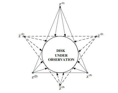
where $r$ is the radius of the circular torus tube, and $R$ is the distance from the torus center to the center of the tube satisfying $R>r$. The observation points are restricted to the exterior of $\mathcal{O}$ and its boundary surface $\partial \mathcal{O}$. Moreover, we require that the distances of the observation points $z^{(i)}$ from the torus center are $>R+r$ and $\leq \Delta$, a specified distance $>R+r$ (See Fig. 3.10). This case is relevant to the problem of sensor placement for observing a toroidal plasma such as that in the tokamak machine. The solution to Problem $3.4$ can be constructed by making use of the geometric symmetry of the torus with respect to the $x_{3}$-axis. To obtain the largest visible sets for each observation point, two of the point observers $z^{(1)}$ and $z^{(2)}$ should be at the maximum allowable distance $\Delta$ from the torus center on the $x_{3}$-axis. The visible sets of these observation points are given by
$$
\mathcal{V}\left(z^{(1)}\right)=\left{\left(x_{1}, x_{2}, x_{3}\right) \in \mathbb{R}^{3}: x_{3}=\sqrt{r^{2}-\left(R-\sqrt{x_{1}^{2}+x_{2}^{2}}\right.}\right)^{2}
$$
if $\left(R-r \cos \left(\theta_{4}\right)\right)^{2}<x_{1}^{2}+x_{2}^{2} \leq\left(R+r \cos \left(\theta_{3}\right)\right)^{2}$;
$$
\left.x_{3}^{2}=r^{2}-\left(R^{2}-\sqrt{x_{1}^{2}+x_{2}^{2}}\right)^{2}, \text { if } r^{2} \leq x_{1}^{2}+x_{2}^{2} \leq\left(R-r \cos \left(\theta_{4}\right)\right)^{2}\right},
$$
$$
\mathcal{V}\left(z^{(2)}\right)=\left{\left(x_{1}, x_{2}, x_{3}\right) \in \mathbb{R}^{3}: x_{3}=-\sqrt{r^{2}-\left(R-\sqrt{x_{1}^{2}+x_{2}^{2}}\right)^{2}}\right.
$$
if $\left(R-r \cos \left(\theta_{4}\right)\right)^{2}<x_{1}^{2}+x_{2}^{2} \leq\left(R+r \cos \left(\theta_{3}\right)\right)^{2}$;
$$
\left.x_{3}^{2}=r^{2}-\left(R^{2}-\sqrt{x_{1}^{2}+x_{2}^{2}}\right)^{2}, \text { if } r^{2} \leq x_{1}^{2}+x_{2}^{2} \leq\left(R-r \cos \left(\theta_{4}\right)\right)^{2}\right},
$$
where
$$
\theta_{1}=\tan ^{-1}(\Delta / R), \quad \theta_{2}=\cos ^{-1}\left(r / \sqrt{\Delta^{2}+R^{2}}\right), \quad \theta_{3}=\pi-\theta_{1}-\theta_{2}, \quad \theta_{4}=\theta_{2}-\theta_{1} .
$$
The invisible set of these points corresponds to $\partial \mathcal{O}-\left(\mathcal{V}\left(z^{(1)}\right) \cup \mathcal{V}\left(z^{(2)}\right)\right)$ which is a circular band given by
$$
\begin{array}{r}
B_{d}=\left{\left(x_{1}, x_{2}, x_{3}\right) \in \mathbb{R}^{3}: x_{3}^{2}=r^{2}-\left(R-\sqrt{x_{1}^{2}+x_{2}^{2}}\right)^{2},\right. \
\text { if } \left.\left(R-r \cos \left(\theta_{3}\right)\right)^{2} \leq x_{1}^{2}+x_{2}^{2} \leq(R+r)^{2}\right}
\end{array}
$$
The remaining problem is determine the minimum number of point-observers at distance $\Delta$ from the torus center to attain total visibility of $B_{d}$. This problem corresponds to finding a $N$-polygon whose vertices lie on the circle $\left{\left(x_{1}, x_{2}, x_{3}\right) \in \mathbb{R}^{3}\right.$ : $\left.x_{1}^{2}+x_{2}^{2}=\Delta^{2}, x_{3}=0\right}$ with the smallest $N$, that circumscribes the circle with radius $R+r$. The minimum number of point-observers for total visibility of $\partial \mathcal{O}$ is $2+N$. Figure $3.10$ shows the location of the point-observers for total visibility of $\partial \mathcal{O}$ for a special case. In this case, the circle $\left{\left(x_{1}, x_{2}, x_{3}\right) \in \mathbb{R}^{3}: x_{1}^{2}+x_{2}^{2}=(R+r)^{2}, x_{3}=0\right}$ can be circumscribed by a square whose corners correspond to the point-observers at a distance $\Delta$ from the torus center. Thus, the minimum number of point-observers for total visibility of $\partial \mathcal{O}$ is six.
Next, we consider a variation of the foregoing case in which the object under observation is a toroidal cavity whose wall is described by (3.20). It is desirable to observe the cavity wall by means of point-observers located on the wall and in the interior of the cavity. We may classify this case as an “Interior Observation-Point Set Problem”, and the former case as an “Exterior Observation-Point Set Problem”.
寻路算法代写
robotics代写|寻路算法代写Path Planning Algorithms|Single Point-Observer Static Optimal Visibility Problems
考虑观察对象的最简单情况这和观景台磷分别是指定实值的图C1-职能F=F(X)和G=G(X)定义于Ω,一个简单连通的紧子集Rn,n∈1,2这样
G(X)>F(X) 对全部 X∈Ω
如备注 2.3 所述,具有实际意义的特殊观测平台是对应于高架剖面的恒定垂直高度平台。F由图定义FH在= 定义 F+H在, 在哪里H在是一个给定的正数,指定上面的点观察者的垂直高度\mathcal{O}=G_{f} \stackrel{\text { def }}{=}\left{(x, f(x)) \in \mathbb{R}^{n+1}\right.$ : $x \in \Omega}\mathcal{O}=G_{f} \stackrel{\text { def }}{=}\left{(x, f(x)) \in \mathbb{R}^{n+1}\right.$ : $x \in \Omega}. 自从F是一个C1-在紧集上定义的函数Ω,GF也很紧凑。此外,对于任何点观察者(X,G(X))∈GG,其可见集在((X,G(X)))及其上的投影Ω(表示为圆周率Ω在((X,G(X)))) 是紧凑的。因此,我们可以认为(X,G(X))→在((X,G(X)))(分别。圆周率Ω在((X,G(X))))作为集值映射GG进入2GF(分别。2Ω). 一般来说,在((X,G(X)))和圆周率Ω(在((X,G(X))))可能是不相交紧凑子集的并集GF和Ω分别。这种情况由图 1 所示的示例说明。3.1与点观察员在(X这,G(X这))∈GG和
Ω=[0,1]. 可以看出\Pi_{\Omega} \mathcal{V}\left(\left(x_{o}, g\left(x_{o}\right)\right)\right)=\left[0, \hat{x} {1}\right] \cup\left{\hat{x}{2}\right} \cup\left[\hat{x}{3}, \hat{x}{4}\right] \cup\左[\hat{x}{5}, \hat{x}{6}\right]\Pi_{\Omega} \mathcal{V}\left(\left(x_{o}, g\left(x_{o}\right)\right)\right)=\left[0, \hat{x} {1}\right] \cup\left{\hat{x}{2}\right} \cup\left[\hat{x}{3}, \hat{x}{4}\right] \cup\左[\hat{x}{5}, \hat{x}{6}\right]与示例 2.1 一样,该示例还表明点观察器的可见集可能包含孤立点。
现在,我们考虑与观察对象相关的两个最佳可见性问题这=GF来自位于 Epi 的点观察员F, 题词F.
问题 3.1 最小垂直高度总能见度问题。给定F= F(X)定义于Ω, 找到最小垂直高度H在≥0和一点X∈Ω这样GF从点观察者处完全可见(X,FH在(X∗)).
问题 3.2 最大能见度问题。给定实值C1-职能F和G定义于Ω满足条件(3.1),找一个点X∈Ω这样ĴG(X)≥ ĴG(X)对全部X∈Ω, 在哪里J_{g}(x) \stackrel{\text { def }}{=} \mu_{1}\left{\Pi_{\Omega} \mathcal{V}((x, g(x)))\right }J_{g}(x) \stackrel{\text { def }}{=} \mu_{1}\left{\Pi_{\Omega} \mathcal{V}((x, g(x)))\right },勒贝格测度圆周率Ω在((X,G(X))).
如果我们设置G在问题3.2到FH在对于给定的H在>0,那么我们就有了实际重要的恒定垂直高度最大能见度问题。
备注 3.1 在问题 3.2 中,我们可以选择最大化在((X,G(X)))而不是总的衡量标准圆周率Ω在((X,G(X)))以增加计算复杂性为代价。
为了解决想法,我们首先考虑一维域的情况的上述问题Ω并给出了一些与解决更一般的最优能见度问题相关的结果。然后,对于二维的情况,类似的问题Ω将被讨论。
robotics代写|寻路算法代写Path Planning Algorithms|Multiple Point-Observer Static Optimal Visibility Problems
到目前为止,我们已经考虑了涉及单个静止点观察器的各种最佳可见性问题。当观察对象的总能见度不能
由单个静止点观察者实现,很自然地要问是否可以通过有限(最好是最小)数量的静止点观察者来获得总能见度。在回答这个问题之前,我们首先建立一些可见集的属性,这些属性在后续开发中很有用。为了简化我们的讨论,我们考虑对象的情况这被观察的是一个表面R3由描述GF, 实值连续函数图F=F(X)定义于Ω, 的紧凑子集R2. 观测点被限制在一个恒定垂直高度的观测平台上磷H在=GF+H在 *
引理3.4每一点X′∈Ω是集值映射的不动点X→ 圆周率Ω在((X,FH和(X)))在Ω进入2Ω. 此外,在某一点X′∈Ω映射在哪里圆周率Ων(⋅,FH在(⋅))关于欧几里得度量是连续的ρ和在Ω, 和豪斯多夫度量ρH在2Ω, 存在一个空位球\mathcal{B}\left(x^{\prime} ; \delta\right)=\left{x \in \mathbb{R}^{2}:\left|xx^{\prime}\right|< \right.$ $\delta}\mathcal{B}\left(x^{\prime} ; \delta\right)=\left{x \in \mathbb{R}^{2}:\left|xx^{\prime}\right|< \right.$ $\delta}关于X′带半径d>0这样(乙(X′;d)∩Ω)⊂圆周率Ω在((X′,FH在(X′))).
证明让X′在任何一点Ω. 那么,重点(X′,F(X′))从该点始终可见(X′,FH在(X′))∈和F. 因此,(X′,F(X′))∈在((X′,FH在(X′))), 和X′∈ 圆周率Ω在((X′,FH在(X′))), 或者X′是一个不动点圆周率Ω在((⋅,FH在(⋅))). 在某一点X′∈Ω映射在哪里圆周率Ω在(⋅,FH在(⋅))关于度量是连续的ρ和和ρH, 存在一个空位球乙(X′;d)带半径d>0这样对于每个X∈乙(X′;d)∩Ω, 点(X,F(X))从可见(X,FH在(X)). 因此,期望的结果如下。
定理3.3假设空间域Ω有一个C1-边界∂Ω, 和映射X→圆周率Ω在((X,FH在(X)))从∂Ω进入2Ω关于度量是连续的ρ和和ρH. 那么存在一个整数ñ≥1, 和一个有限点集P(N)=\left{x^{(k)}, k=1, \ldots, N\right} \subset \OmegaP(N)=\left{x^{(k)}, k=1, \ldots, N\right} \subset \Omega这样Ω=⋃ķ=1ñ圆周率Ω在((X(ķ),FH在(X(ķ)))),或等效地,GF从有限点集中完全可见\left{\left(x^{(k)}, f_{h_{v}}\left(x^{(k)}\right)\right): x^{(k)} \in\right。 $ $\left.P^{(N)}\right} 。\left{\left(x^{(k)}, f_{h_{v}}\left(x^{(k)}\right)\right): x^{(k)} \in\right。 $ $\left.P^{(N)}\right} 。
证明自∂Ω是C1紧凑;和F受限于∂Ω是一个C1-函数,它遵循引理2.1我们可以找到一个有限点集P_{1}=\left{x^{(k)} \in \partial \Omega, k=1, \ldots, M\right}P_{1}=\left{x^{(k)} \in \partial \Omega, k=1, \ldots, M\right}这样⋃ķ=1米乙(X(ķ);d分钟)形成边界层大号乙关于∂Ω, 在哪里d分钟是开球的最小半径乙(X;d)(具有引理 3.4 中指定的属性)X∈∂Ω, 和
大号乙=⋃ķ=1米(乙(X(ķ);d分钟)∩Ω)
robotics代写|寻路算法代写Path Planning Algorithms|Non-simply Connected Objects
对于 3D 非简单连接的对象,确定总可见性的最小点观察者数量通常是一个难题。我们将研究几个问题的明确解决方案3.4是可获得的。
(i) 环形物体:首先,考虑固体物体的情况这谁的表面∂这在观察中是一个3−D圆环描述为:
\partial \mathcal{O}=\left{\left(x_{1}, x_{2}, x_{3}\right) \in \mathbb{R}^{3}: x_{3}^{2 }=r^{2}-\left(R-\sqrt{x_{1}^{2}+x_{2}^{2}}\right)^{2}\right}\partial \mathcal{O}=\left{\left(x_{1}, x_{2}, x_{3}\right) \in \mathbb{R}^{3}: x_{3}^{2 }=r^{2}-\left(R-\sqrt{x_{1}^{2}+x_{2}^{2}}\right)^{2}\right}
在哪里r是圆环管的半径,和R是从圆环中心到管中心的距离,满足R>r. 观察点仅限于外部这及其边界面∂这. 此外,我们要求观察点的距离和(一世)从圆环中心是>R+r和≤Δ, 指定距离>R+r(见图 3.10)。这种情况与用于观察环形等离子体(例如托卡马克机中的等离子体)的传感器放置问题有关。问题的解决方案3.4可以利用环面的几何对称性来构造X3-轴。为了获得每个观察点的最大可见集,两个点观察者和(1)和和(2)应该在最大允许距离Δ从圆环中心X3-轴。这些观察点的可见集由下式给出\mathcal{V}\left(z^{(1)}\right)=\left{\left(x_{1}, x_{2}, x_{3}\right) \in \mathbb{R}^ {3}:x_{3}=\sqrt{r^{2}-\left(R-\sqrt{x_{1}^{2}+x_{2}^{2}}\right.}\right )^{2} $$ if $\left(Rr \cos \left(\theta_{4}\right)\right)^{2}<x_{1}^{2}+x_{2}^{2 } \leq\left(R+r \cos \left(\theta_{3}\right)\right)^{2}$; $$ \left.x_{3}^{2}=r^{2}-\left(R^{2}-\sqrt{x_{1}^{2}+x_{2}^{2}} \right)^{2}, \text { if } r^{2} \leq x_{1}^{2}+x_{2}^{2} \leq\left(Rr \cos \left(\theta_ {4}\right)\right)^{2}\right},\mathcal{V}\left(z^{(1)}\right)=\left{\left(x_{1}, x_{2}, x_{3}\right) \in \mathbb{R}^ {3}:x_{3}=\sqrt{r^{2}-\left(R-\sqrt{x_{1}^{2}+x_{2}^{2}}\right.}\right )^{2} $$ if $\left(Rr \cos \left(\theta_{4}\right)\right)^{2}<x_{1}^{2}+x_{2}^{2 } \leq\left(R+r \cos \left(\theta_{3}\right)\right)^{2}$; $$ \left.x_{3}^{2}=r^{2}-\left(R^{2}-\sqrt{x_{1}^{2}+x_{2}^{2}} \right)^{2}, \text { if } r^{2} \leq x_{1}^{2}+x_{2}^{2} \leq\left(Rr \cos \left(\theta_ {4}\right)\right)^{2}\right},
\mathcal{V}\left(z^{(2)}\right)=\left{\left(x_{1}, x_{2}, x_{3}\right) \in \mathbb{R}^ {3}:x_{3}=-\sqrt{r^{2}-\left(R-\sqrt{x_{1}^{2}+x_{2}^{2}}\right)^{ 2}}\对。$$ if $\left(Rr \cos \left(\theta_{4}\right)\right)^{2}<x_{1}^{2}+x_{2}^{2} \leq\left (R+r \cos \left(\theta_{3}\right)\right)^{2}$; $$ \left.x_{3}^{2}=r^{2}-\left(R^{2}-\sqrt{x_{1}^{2}+x_{2}^{2}} \right)^{2}, \text { if } r^{2} \leq x_{1}^{2}+x_{2}^{2} \leq\left(Rr \cos \left(\theta_ {4}\right)\right)^{2}\right},\mathcal{V}\left(z^{(2)}\right)=\left{\left(x_{1}, x_{2}, x_{3}\right) \in \mathbb{R}^ {3}:x_{3}=-\sqrt{r^{2}-\left(R-\sqrt{x_{1}^{2}+x_{2}^{2}}\right)^{ 2}}\对。$$ if $\left(Rr \cos \left(\theta_{4}\right)\right)^{2}<x_{1}^{2}+x_{2}^{2} \leq\left (R+r \cos \left(\theta_{3}\right)\right)^{2}$; $$ \left.x_{3}^{2}=r^{2}-\left(R^{2}-\sqrt{x_{1}^{2}+x_{2}^{2}} \right)^{2}, \text { if } r^{2} \leq x_{1}^{2}+x_{2}^{2} \leq\left(Rr \cos \left(\theta_ {4}\right)\right)^{2}\right},
在哪里
θ1=棕褐色−1(Δ/R),θ2=因−1(r/Δ2+R2),θ3=圆周率−θ1−θ2,θ4=θ2−θ1.
这些点的不可见集合对应于∂这−(在(和(1))∪在(和(2)))这是一个圆形带
\begin{array}{r} B_{d}=\left{\left(x_{1}, x_{2}, x_{3}\right) \in \mathbb{R}^{3}: x_{ 3}^{2}=r^{2}-\left(R-\sqrt{x_{1}^{2}+x_{2}^{2}}\right)^{2},\right. \ \text { if } \left.\left(Rr \cos \left(\theta_{3}\right)\right)^{2} \leq x_{1}^{2}+x_{2}^{ 2} \leq(R+r)^{2}\right} \end{数组}\begin{array}{r} B_{d}=\left{\left(x_{1}, x_{2}, x_{3}\right) \in \mathbb{R}^{3}: x_{ 3}^{2}=r^{2}-\left(R-\sqrt{x_{1}^{2}+x_{2}^{2}}\right)^{2},\right. \ \text { if } \left.\left(Rr \cos \left(\theta_{3}\right)\right)^{2} \leq x_{1}^{2}+x_{2}^{ 2} \leq(R+r)^{2}\right} \end{数组}
剩下的问题是确定距离点观察者的最小数量Δ从圆环中心获得总能见度乙d. 这个问题对应于找到一个ñ- 顶点位于圆上的多边形\left{\left(x_{1}, x_{2}, x_{3}\right) \in \mathbb{R}^{3}\right.$ : $\left.x_{1}^{2 }+x_{2}^{2}=\Delta^{2}, x_{3}=0\right}\left{\left(x_{1}, x_{2}, x_{3}\right) \in \mathbb{R}^{3}\right.$ : $\left.x_{1}^{2 }+x_{2}^{2}=\Delta^{2}, x_{3}=0\right}用最小的ñ, 以半径外接圆R+r. 总能见度的最小观察点数∂这是2+ñ. 数字3.10显示点观察者的位置,以获得总可见性∂这对于特殊情况。在这种情况下,圆\left{\left(x_{1}, x_{2}, x_{3}\right) \in \mathbb{R}^{3}: x_{1}^{2}+x_{2}^{ 2}=(R+r)^{2}, x_{3}=0\right}\left{\left(x_{1}, x_{2}, x_{3}\right) \in \mathbb{R}^{3}: x_{1}^{2}+x_{2}^{ 2}=(R+r)^{2}, x_{3}=0\right}可以被一个正方形包围,其角对应于远处的点观察者Δ从圆环中心。因此,总能见度的最小观察点数∂这是六。
接下来,我们考虑上述情况的变体,其中观察对象是一个环形腔,其壁由(3.20)描述。理想的是通过位于壁上和空腔内部的点观察器来观察空腔壁。我们可以将这种情况归类为“内部观测点集问题”,将前一种情况归类为“外部观测点集问题”。

统计代写请认准statistics-lab™. statistics-lab™为您的留学生涯保驾护航。
金融工程代写
金融工程是使用数学技术来解决金融问题。金融工程使用计算机科学、统计学、经济学和应用数学领域的工具和知识来解决当前的金融问题,以及设计新的和创新的金融产品。
非参数统计代写
非参数统计指的是一种统计方法,其中不假设数据来自于由少数参数决定的规定模型;这种模型的例子包括正态分布模型和线性回归模型。
广义线性模型代考
广义线性模型(GLM)归属统计学领域,是一种应用灵活的线性回归模型。该模型允许因变量的偏差分布有除了正态分布之外的其它分布。
术语 广义线性模型(GLM)通常是指给定连续和/或分类预测因素的连续响应变量的常规线性回归模型。它包括多元线性回归,以及方差分析和方差分析(仅含固定效应)。
有限元方法代写
有限元方法(FEM)是一种流行的方法,用于数值解决工程和数学建模中出现的微分方程。典型的问题领域包括结构分析、传热、流体流动、质量运输和电磁势等传统领域。
有限元是一种通用的数值方法,用于解决两个或三个空间变量的偏微分方程(即一些边界值问题)。为了解决一个问题,有限元将一个大系统细分为更小、更简单的部分,称为有限元。这是通过在空间维度上的特定空间离散化来实现的,它是通过构建对象的网格来实现的:用于求解的数值域,它有有限数量的点。边界值问题的有限元方法表述最终导致一个代数方程组。该方法在域上对未知函数进行逼近。[1] 然后将模拟这些有限元的简单方程组合成一个更大的方程系统,以模拟整个问题。然后,有限元通过变化微积分使相关的误差函数最小化来逼近一个解决方案。
tatistics-lab作为专业的留学生服务机构,多年来已为美国、英国、加拿大、澳洲等留学热门地的学生提供专业的学术服务,包括但不限于Essay代写,Assignment代写,Dissertation代写,Report代写,小组作业代写,Proposal代写,Paper代写,Presentation代写,计算机作业代写,论文修改和润色,网课代做,exam代考等等。写作范围涵盖高中,本科,研究生等海外留学全阶段,辐射金融,经济学,会计学,审计学,管理学等全球99%专业科目。写作团队既有专业英语母语作者,也有海外名校硕博留学生,每位写作老师都拥有过硬的语言能力,专业的学科背景和学术写作经验。我们承诺100%原创,100%专业,100%准时,100%满意。
随机分析代写
随机微积分是数学的一个分支,对随机过程进行操作。它允许为随机过程的积分定义一个关于随机过程的一致的积分理论。这个领域是由日本数学家伊藤清在第二次世界大战期间创建并开始的。
时间序列分析代写
随机过程,是依赖于参数的一组随机变量的全体,参数通常是时间。 随机变量是随机现象的数量表现,其时间序列是一组按照时间发生先后顺序进行排列的数据点序列。通常一组时间序列的时间间隔为一恒定值(如1秒,5分钟,12小时,7天,1年),因此时间序列可以作为离散时间数据进行分析处理。研究时间序列数据的意义在于现实中,往往需要研究某个事物其随时间发展变化的规律。这就需要通过研究该事物过去发展的历史记录,以得到其自身发展的规律。
回归分析代写
多元回归分析渐进(Multiple Regression Analysis Asymptotics)属于计量经济学领域,主要是一种数学上的统计分析方法,可以分析复杂情况下各影响因素的数学关系,在自然科学、社会和经济学等多个领域内应用广泛。
MATLAB代写
MATLAB 是一种用于技术计算的高性能语言。它将计算、可视化和编程集成在一个易于使用的环境中,其中问题和解决方案以熟悉的数学符号表示。典型用途包括:数学和计算算法开发建模、仿真和原型制作数据分析、探索和可视化科学和工程图形应用程序开发,包括图形用户界面构建MATLAB 是一个交互式系统,其基本数据元素是一个不需要维度的数组。这使您可以解决许多技术计算问题,尤其是那些具有矩阵和向量公式的问题,而只需用 C 或 Fortran 等标量非交互式语言编写程序所需的时间的一小部分。MATLAB 名称代表矩阵实验室。MATLAB 最初的编写目的是提供对由 LINPACK 和 EISPACK 项目开发的矩阵软件的轻松访问,这两个项目共同代表了矩阵计算软件的最新技术。MATLAB 经过多年的发展,得到了许多用户的投入。在大学环境中,它是数学、工程和科学入门和高级课程的标准教学工具。在工业领域,MATLAB 是高效研究、开发和分析的首选工具。MATLAB 具有一系列称为工具箱的特定于应用程序的解决方案。对于大多数 MATLAB 用户来说非常重要,工具箱允许您学习和应用专业技术。工具箱是 MATLAB 函数(M 文件)的综合集合,可扩展 MATLAB 环境以解决特定类别的问题。可用工具箱的领域包括信号处理、控制系统、神经网络、模糊逻辑、小波、仿真等。