
如果你也在 怎样代写统计推断Statistical Inference 这个学科遇到相关的难题,请随时右上角联系我们的24/7代写客服。统计推断Statistical Inference是利用数据分析来推断概率基础分布的属性的过程。推断性统计分析推断人口的属性,例如通过测试假设和得出估计值。假设观察到的数据集是从一个更大的群体中抽出的。
统计推断Statistical Inference(可以与描述性统计进行对比。描述性统计只关注观察到的数据的属性,它并不依赖于数据来自一个更大的群体的假设。在机器学习中,推理一词有时被用来代替 “通过评估一个已经训练好的模型来进行预测”;在这种情况下,推断模型的属性被称为训练或学习(而不是推理),而使用模型进行预测被称为推理(而不是预测);另见预测推理。
statistics-lab™ 为您的留学生涯保驾护航 在代写统计推断Statistical inference方面已经树立了自己的口碑, 保证靠谱, 高质且原创的统计Statistics代写服务。我们的专家在代写统计推断Statistical inference代写方面经验极为丰富,各种代写统计推断Statistical inference相关的作业也就用不着说。
统计代写|统计推断代写Statistical inference代考|Visualization of Data
There are two main methods of visualizing data, and several others that are related to these methods. In this section we introduce just two, histograms and scatter plots, and we will use these throughout the text.
Histograms
Histograms are a way of summarizing data, when presenting the entire data set is impractical, or where some understanding of the data is made clearer by summarizing. The histogram plot is done with the following steps:
1 Choose a number of bins to divide the data.
2 Count up the data that fall into each bin
3 Make a bar plot, or a scatter plot to present the data.
The following is an example with a small data set. The process of binning and counting is often done by computer, but it is instructive to perform the process by hand a few times in order to understand what the results are.
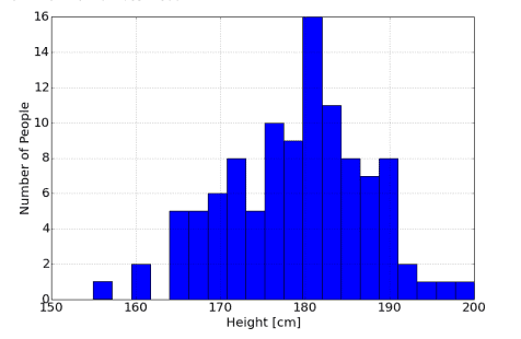
Table 3.3 shows a collection of 106 heights (in centimeters) of the male students in a class’. As a collection of numbers it is relatively opaque, but as a histogram it is clearer.
From this histogram, we can immediately observe several quantities which summarize their data:
1 The average value (around the middle) should be around $175 \mathrm{~cm}$. The actual value can be calculated from the data, as
$$
\bar{x}=\frac{177.8+160.0+\cdots+180.34+183.0}{106}=178.83
$$
2 The range of the data is around $155 \mathrm{~cm}$ up to about $205 \mathrm{~cm}$. Again we can be more precise, and find the minimum of the data (154.94 $\mathrm{cm}$ ) and the maximum $(200 \mathrm{~cm}$ ) but the histogram picture yields an approximate value instantly.
3 The values are roughly symmetric about the mean (i.e. average) value. This can give us a clue concerning how to model the data.
What is quite clear is that it is far easier to deal with a histogram, as above, than find the same information from the table of numbers.
统计代写|统计推断代写Statistical inference代考|Computer Examples
This section summarizes how to make histograms and scatter plots with the computer software.
Histograms
from sie import *
Load a sample data set, and select only the Male data…
$$
\begin{aligned}
& \text { data=load_data (‘data/survey .csv’) } \
& \text { male_data=data [data [‘Sex’]== ‘Male’] }
\end{aligned}
$$
select only the height data, and drop the missing data (na)…
$$
\text { male_height }=\text { male_data [ ‘Height’]. dropna() }
$$
make the histogram
$$
\begin{aligned}
& \text { hist (male_height, bins }=20) \
& \text { xlabel (‘Height [cm]’) } \
& \text { ylabel (‘Number of People’) }
\end{aligned}
$$
$
data=load_data(‘data/survey.csv’)
male_data=data $[$ data [‘Sex’ $]==$ ‘Male’]
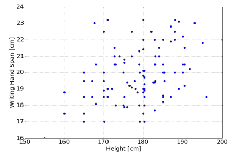
select only the height and the width of writing hand data, and drop the missing data (na)…
subdata=male_data [[ ‘Height’, ‘Wr.Hnd’]].dropna ()
height=subdata [‘Height’]
wr_hand=subdata [ ‘Wr.Hnd’]
plot the data
plot (height,wr_hand, ‘o’)
ylabel (‘Writing Hand Span [cm]’)
xlabel (‘Height [cm]’)
$
统计推断代考
统计代写|统计推断代写Statistical inference代考|Visualization of Data
有两种主要的数据可视化方法,以及与这些方法相关的其他几种方法。在本节中,我们只介绍两种,直方图和散点图,我们将在整个文本中使用它们。
直方图
当呈现整个数据集是不切实际的,或者通过汇总可以更清楚地理解数据时,直方图是一种汇总数据的方式。直方图的绘制步骤如下:
1选择若干个bin对数据进行划分。
把每个箱子里的数据加起来
制作条形图或散点图来表示数据。
下面是一个小数据集的例子。装箱和计数的过程通常是由计算机完成的,但为了了解结果是什么,手工执行几次这个过程是有指导意义的。
表3.3是某班级男生身高(厘米)106的汇总。作为一组数字,它相对不透明,但作为一个直方图,它更清晰。
从这个直方图中,我们可以立即观察到总结其数据的几个量:
1平均值(中间左右)应在$175 \mathrm{~cm}$左右。实际值可由数据计算得出,为
$$
\bar{x}=\frac{177.8+160.0+\cdots+180.34+183.0}{106}=178.83
$$
2数据范围在$155 \mathrm{~cm}$ ~ $205 \mathrm{~cm}$左右。同样,我们可以更精确地找到数据的最小值(154.94 $\mathrm{cm}$)和最大值$(200 \mathrm{~cm}$),但直方图立即产生一个近似值。
这些值大致对称于平均值(即平均值)。这可以给我们一个关于如何对数据建模的线索。
很明显,处理直方图要比从数字表中找到相同的信息容易得多。
统计代写|统计推断代写Statistical inference代考|Computer Examples
本节总结了如何用计算机软件制作直方图和散点图。
直方图
源自sie import *
加载一个样本数据集,并只选择Male数据…
$$
\begin{aligned}
& \text { data=load_data (‘data/survey .csv’) } \
& \text { male_data=data [data [‘Sex’]== ‘Male’] }
\end{aligned}
$$
只选择高度数据,并删除缺失的数据(na)…
$$
\text { male_height }=\text { male_data [ ‘Height’]. dropna() }
$$
制作直方图
$$
\begin{aligned}
& \text { hist (male_height, bins }=20) \
& \text { xlabel (‘Height [cm]’) } \
& \text { ylabel (‘Number of People’) }
\end{aligned}
$$
$
data=load_data(‘data/survey.csv’)
male_data=data $ [$ data [‘Sex’ $]==$ ‘Male’]
select only the height and the width of writing hand data, and drop the missing data (na)…
subdata=male_data [[ ‘Height’, ‘Wr.Hnd’]].dropna ()
height=subdata [‘Height’]
wr_hand=subdata [ ‘Wr.Hnd’]
plot the data
plot (height,wr_hand, ‘o’)
ylabel (‘Writing Hand Span [cm]’)
xlabel (‘Height [cm]’)
$

统计代写请认准statistics-lab™. statistics-lab™为您的留学生涯保驾护航。
金融工程代写
金融工程是使用数学技术来解决金融问题。金融工程使用计算机科学、统计学、经济学和应用数学领域的工具和知识来解决当前的金融问题,以及设计新的和创新的金融产品。
非参数统计代写
非参数统计指的是一种统计方法,其中不假设数据来自于由少数参数决定的规定模型;这种模型的例子包括正态分布模型和线性回归模型。
广义线性模型代考
广义线性模型(GLM)归属统计学领域,是一种应用灵活的线性回归模型。该模型允许因变量的偏差分布有除了正态分布之外的其它分布。
术语 广义线性模型(GLM)通常是指给定连续和/或分类预测因素的连续响应变量的常规线性回归模型。它包括多元线性回归,以及方差分析和方差分析(仅含固定效应)。
有限元方法代写
有限元方法(FEM)是一种流行的方法,用于数值解决工程和数学建模中出现的微分方程。典型的问题领域包括结构分析、传热、流体流动、质量运输和电磁势等传统领域。
有限元是一种通用的数值方法,用于解决两个或三个空间变量的偏微分方程(即一些边界值问题)。为了解决一个问题,有限元将一个大系统细分为更小、更简单的部分,称为有限元。这是通过在空间维度上的特定空间离散化来实现的,它是通过构建对象的网格来实现的:用于求解的数值域,它有有限数量的点。边界值问题的有限元方法表述最终导致一个代数方程组。该方法在域上对未知函数进行逼近。[1] 然后将模拟这些有限元的简单方程组合成一个更大的方程系统,以模拟整个问题。然后,有限元通过变化微积分使相关的误差函数最小化来逼近一个解决方案。
tatistics-lab作为专业的留学生服务机构,多年来已为美国、英国、加拿大、澳洲等留学热门地的学生提供专业的学术服务,包括但不限于Essay代写,Assignment代写,Dissertation代写,Report代写,小组作业代写,Proposal代写,Paper代写,Presentation代写,计算机作业代写,论文修改和润色,网课代做,exam代考等等。写作范围涵盖高中,本科,研究生等海外留学全阶段,辐射金融,经济学,会计学,审计学,管理学等全球99%专业科目。写作团队既有专业英语母语作者,也有海外名校硕博留学生,每位写作老师都拥有过硬的语言能力,专业的学科背景和学术写作经验。我们承诺100%原创,100%专业,100%准时,100%满意。
随机分析代写
随机微积分是数学的一个分支,对随机过程进行操作。它允许为随机过程的积分定义一个关于随机过程的一致的积分理论。这个领域是由日本数学家伊藤清在第二次世界大战期间创建并开始的。
时间序列分析代写
随机过程,是依赖于参数的一组随机变量的全体,参数通常是时间。 随机变量是随机现象的数量表现,其时间序列是一组按照时间发生先后顺序进行排列的数据点序列。通常一组时间序列的时间间隔为一恒定值(如1秒,5分钟,12小时,7天,1年),因此时间序列可以作为离散时间数据进行分析处理。研究时间序列数据的意义在于现实中,往往需要研究某个事物其随时间发展变化的规律。这就需要通过研究该事物过去发展的历史记录,以得到其自身发展的规律。
回归分析代写
多元回归分析渐进(Multiple Regression Analysis Asymptotics)属于计量经济学领域,主要是一种数学上的统计分析方法,可以分析复杂情况下各影响因素的数学关系,在自然科学、社会和经济学等多个领域内应用广泛。
MATLAB代写
MATLAB 是一种用于技术计算的高性能语言。它将计算、可视化和编程集成在一个易于使用的环境中,其中问题和解决方案以熟悉的数学符号表示。典型用途包括:数学和计算算法开发建模、仿真和原型制作数据分析、探索和可视化科学和工程图形应用程序开发,包括图形用户界面构建MATLAB 是一个交互式系统,其基本数据元素是一个不需要维度的数组。这使您可以解决许多技术计算问题,尤其是那些具有矩阵和向量公式的问题,而只需用 C 或 Fortran 等标量非交互式语言编写程序所需的时间的一小部分。MATLAB 名称代表矩阵实验室。MATLAB 最初的编写目的是提供对由 LINPACK 和 EISPACK 项目开发的矩阵软件的轻松访问,这两个项目共同代表了矩阵计算软件的最新技术。MATLAB 经过多年的发展,得到了许多用户的投入。在大学环境中,它是数学、工程和科学入门和高级课程的标准教学工具。在工业领域,MATLAB 是高效研究、开发和分析的首选工具。MATLAB 具有一系列称为工具箱的特定于应用程序的解决方案。对于大多数 MATLAB 用户来说非常重要,工具箱允许您学习和应用专业技术。工具箱是 MATLAB 函数(M 文件)的综合集合,可扩展 MATLAB 环境以解决特定类别的问题。可用工具箱的领域包括信号处理、控制系统、神经网络、模糊逻辑、小波、仿真等。