如果你也在 怎样代写变分法variational methods这个学科遇到相关的难题，请随时右上角联系我们的24/7代写客服。

变分法是一种数学方法，用于近似计算困难量子系统的能级。它也可以用来近似计算一个可解系统的能量，然后通过比较已知和近似的能量来获得方法的准确性。

statistics-lab™ 为您的留学生涯保驾护航 在代写变分法variational methods方面已经树立了自己的口碑, 保证靠谱, 高质且原创的统计Statistics代写服务。我们的专家在代写变分法variational methods代写方面经验极为丰富，各种代写变分法variational methods相关的作业也就用不着说。

我们提供的变分法variational methods及其相关学科的代写，服务范围广, 其中包括但不限于:

• Statistical Inference 统计推断
• Statistical Computing 统计计算
• Advanced Probability Theory 高等概率论
• Advanced Mathematical Statistics 高等数理统计学
• (Generalized) Linear Models 广义线性模型
• Statistical Machine Learning 统计机器学习
• Longitudinal Data Analysis 纵向数据分析
• Foundations of Data Science 数据科学基础

数学代写|变分法代写variational methods代考|Sufficient Statistics

When working with statistical models, it is necessary to recover some, or even all, of its parameters from a set of randomly drawn samples $x_1, x_2, \cdots, x_n$. Assuming these observations are iid and sampled from a PDF $f(x ; \theta)$, estimating the parameter $\theta$ is the goal of many statisticians and engineers, imposing a real challenge sometimes. A rather common approach is to capture and summarize some information from the observations and use it to estimate the parameter $\boldsymbol{\theta}$ instead of using the observations themselves. This strategy is known as data reduction, whereas engineers and computer scientists call it feature extraction.

The problem of the data reduction is the loss of information. How do we guarantee that with the statistics we computed from the observations, call it $T(\mathbf{X})$, we are not discarding information to estimate $\theta$ ? The answer to this question is provided by the Sufficiency Principle, which defines $T(\mathbf{X})$ as a sufficient statistics when, for any two samples $\mathbf{x}_1$ and $\mathbf{x}_2$, where $T\left(\mathbf{x}_1\right)=T\left(\mathbf{x}_2\right)$, the estimation of $\theta$ yields the same results despite observing $\mathbf{X}=\mathbf{x}_1$ or $\mathbf{X}=\mathbf{x}_2$.

Computing the sufficient statistics for a parameter is a rather difficult task in most scenarios, but a rather simple way to do that is by using the Fisher-Neyman Theorem (also known as factorization theorem).

Theorem $2.2$ (Fisher-Neyman Factorization Theorem) Let $x_1, x_2, \cdots, x_n$ be random observations from a discrete distribution with $P D F f(\mathbf{x} ; \boldsymbol{\theta})$, and $\mathbf{x}=$ $\left[x_1, x_2, \cdots, x_n\right]^t . T(\mathbf{X})$ is a sufficient statistics if, and only if, there exist functions $g(T(\mathbf{x}) ; \boldsymbol{\theta})$ and $h(\mathbf{x})$, such that $h(\mathbf{x}) \geq 0$ and, for all sample points $\mathbf{x}$ and all values of $\boldsymbol{\theta}$, the distribution $f(\mathbf{x} ; \boldsymbol{\theta})$ can be factorized as follows:
$$
f(\mathbf{x} ; \boldsymbol{\theta})-g(T(\mathbf{x}) ; \boldsymbol{\theta}) h(\mathbf{x}) .
$$
For example, for a one-dimensional Poisson distribution with unknown mean $\theta$, if we draw a sample $\mathbf{x}$ formed by $n$ iid observations, it is possible to write the probability function as:
$$
f(\mathbf{x} ; \theta)=\prod_{i=1}^n f\left(x_i ; \theta\right)=\prod_{i=1}^n \frac{e^{-\theta} \theta^{x_i}}{x_{i} !}=\frac{e^{-n \theta} \theta \sum_{i=1}^n x_i}{\prod_{i=1}^n x_{i} !}=g(T(\mathbf{x}) ; \theta) h(\mathbf{x})
$$
where $g(T(\mathbf{x}) ; \theta)=e^{-n \theta} \theta \sum_{i=1}^n x_i$ and $h(\mathbf{x})=\left(\prod_{i=1}^n x_{i} !\right)^{-1}$. So, from the factorization theorem, $T(\mathbf{x})=\sum_{i=1}^n x_i$ is a sufficient statistics for $\theta$.

数学代写|变分法代写variational methods代考|Fisher Information

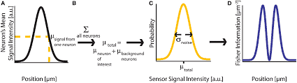
The Fisher information measures the variance in the distribution $f(x ; \theta)$ inflicted by changes in the parameter space $\Theta$. Intuitively, it quantifies the amount of information about $\theta$ that lies in the random variable $X$.

For the $k$-dimensional parameter space $\boldsymbol{\Theta}$ and random variable $\mathbf{X}$ with PDF $f(\mathbf{x} ; \boldsymbol{\theta})$, the elements of the Fisher information matrix are
$$
I_{i, j}(\boldsymbol{\theta})=\operatorname{Cov}\left(\frac{\partial}{\partial \theta_i} \log f(\mathbf{X} ; \boldsymbol{\theta}), \frac{\partial}{\partial \theta_j} \log f(\mathbf{X} ; \boldsymbol{\theta})\right),
$$
where $\operatorname{Cov}(\cdot, \cdot)$ is the covariance function.
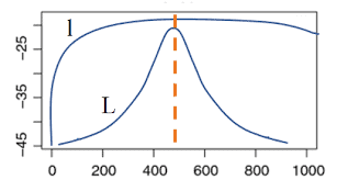
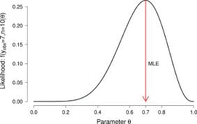
The vector $\frac{\partial}{\partial \theta} \log f(\mathbf{X} ; \boldsymbol{\theta})$ is called the score function and indicates the sensitivity of the likelihood to the parameter $\boldsymbol{\theta}$. When a likelihood $L(\boldsymbol{\theta} \mid \mathbf{x})$, corresponding to the PDF $f(\mathbf{x} ; \boldsymbol{\theta})$, is very sensitive to variations in $\boldsymbol{\theta}$ it is easier to find strong candidates to the true parameter value: even small changes in $\theta$ are enough to cause the likely observations to be considerably different. However, since the score function has mean equal to zero [9], a high $I_{i, j}(\theta)$ implies that the score function is generally high and then, $\mathbf{X}$ distinguishes well the plausible values of $\boldsymbol{\theta}$. We state “generally” because, being the covariance of the score, the Fisher information is an expectation over all possible values of $\mathbf{x}$.

The Fisher information encodes the curvature of the parameter space and plays an important role in optimization. In Chap. 4 we shall see one method that relies on the Fisher information and in Appendix A.4 we show that the Fisher matrix is the negative of the expected value of the Hessian of the log-likelihood.

变分法代写

数学代写|变分法代写variational methods代考|Sufficient Statistics

使用统计模型时，有必要从一组随机抽取的样本中恢复部分甚至全部参数 $x_1, x_2, \cdots, x_n$. 假设这些观察是 $\mathrm{iid}$ 并从 PDF 中采样 $f(x ; \theta)$ ，估计参数 $\theta$ 是许多统计学家和工程师的目标，有时会带来真正的挑战。一种相当常见 的方法是从观察中捕获和总结一些信息，并用它来估计参数 $\theta$ 而不是使用观察结果本身。这种策略被称为数据缩 减，而工程师和计算机科学家称之为特征提取。
数据缩咸的问题是信息丢失。我们如何保证我们从观察中计算出的统计数据，称之为 $T(\mathbf{X})$ ，我们不会丢弃信 息来估计 $\theta$ ? 这个问题的答案是由充足性原则提供的，它定义了 $T(\mathbf{X})$ 作为充分的统计量，对于任意两个样本 $\mathbf{x}1$ 和 $\mathbf{x}_2$ ， 在哪里 $T\left(\mathbf{x}_1\right)=T\left(\mathbf{x}_2\right)$ ，的估计 $\theta$ 尽管观察得到相同的结果 $\mathbf{X}=\mathbf{x}_1$ 或者 $\mathbf{X}=\mathbf{x}_2$. 在大多数情况下，计算参数的充分统计量是一项相当困难的任务，但一种相当简单的方法是使用 FisherNeyman 定理（也称为因式分解定理）。 定理2.2 (Fisher-Neyman 分解定理) 让 $x_1, x_2, \cdots, x_n$ 是来自离散分布的随机观察值 $P D F f(\mathbf{x} ; \boldsymbol{\theta})$ ，和 $\mathbf{x}=\left[x_1, x_2, \cdots, x_n\right]^t . T(\mathbf{X})$ 是充分统计当且仅当存在函数 $g(T(\mathbf{x}) ; \boldsymbol{\theta})$ 和 $h(\mathbf{x})$, 这样 $h(\mathbf{x}) \geq 0$ 并且，对于 所有样本点 $\mathbf{x}$ 和所有值 $\boldsymbol{\theta}$ ，分布 $f(\mathbf{x} ; \boldsymbol{\theta})$ 可以分解如下: $$ f(\mathbf{x} ; \boldsymbol{\theta})-g(T(\mathbf{x}) ; \boldsymbol{\theta}) h(\mathbf{x}) . $$ 例如，对于均值末知的一维泊松分布 $\theta$ ，如果我们抽取样本 $\mathbf{x}$ 由 $n$ iid 观察，可以将概率函数写为: $$ f(\mathbf{x} ; \theta)=\prod{i=1}^n f\left(x_i ; \theta\right)=\prod_{i=1}^n \frac{e^{-\theta} \theta^{x_i}}{x_{i} !}=\frac{e^{-n \theta} \theta \sum_{i=1}^n x_i}{\prod_{i=1}^n x_{i} !}=g(T(\mathbf{x}) ; \theta) h(\mathbf{x})
$$
在哪里 $g(T(\mathbf{x}) ; \theta)=e^{-n \theta} \theta \sum_{i=1}^n x_i$ 和 $h(\mathbf{x})=\left(\prod_{i=1}^n x_{i} !\right)^{-1}$. 所以，根据分解定理， $T(\mathbf{x})=\sum_{i=1}^n x_i$ 是一个充分的统计量 $\theta$.

数学代写|变分法代写variational methods代考|Fisher Information

Fisher 信息衡量分布的方差 $f(x ; \theta)$ 由参数空间的变化引起 $\Theta$. 直观上，它量化了有关的信息量 $\theta$ 在于随机变量 $X$
为了 $k$-维参数空间 $\Theta$ 和随机变量 $\mathbf{X}$ 附PDF $f(\mathbf{x} ; \boldsymbol{\theta})$, Fisher 信息矩阵的元素是
$$
I_{i, j}(\boldsymbol{\theta})=\operatorname{Cov}\left(\frac{\partial}{\partial \theta_i} \log f(\mathbf{X} ; \boldsymbol{\theta}), \frac{\partial}{\partial \theta_j} \log f(\mathbf{X} ; \boldsymbol{\theta})\right),
$$
在哪里Cov $(\cdot, \cdot)$ 是协方差函数。
载体 $\frac{\partial}{\partial \theta} \log f(\mathbf{X} ; \boldsymbol{\theta})$ 称为得分函数，表示似然对参数的敏感度 $\boldsymbol{\theta}$. 当一个可能性 $L(\boldsymbol{\theta} \mid \mathbf{x})$, 对应 $\operatorname{PDF} f(\mathbf{x} ; \boldsymbol{\theta})$ ，对 变化非常敏感 $\theta$ 更容易找到真实参数值的有力候选者: 即使是微小的变化 $\theta$ 足以使可能的观察结果大不相同。然 而，由于得分函数的均值为零 [9]，一个高 $I_{i, j}(\theta)$ 意味着得分函数通常很高，然后， X很好地区分了合理的价值 $\boldsymbol{\theta}$. 我们说“一般“是因为，作为分数的协方差，Fisher 信息是对所有可能值的期望 $\mathbf{x}$.

Fisher 信息对参数空间的曲率进行编码，在优化中起着重要作用。在第一章 在图 4 中，我们将看到一种依赖 Fisher 信息的方法，在附录 A.4 中，我们证明了 Fisher 矩阵是对数似然 Hessian 矩阵期望值的负值。

统计代写请认准statistics-lab™. statistics-lab™为您的留学生涯保驾护航。

金融工程代写

金融工程是使用数学技术来解决金融问题。金融工程使用计算机科学、统计学、经济学和应用数学领域的工具和知识来解决当前的金融问题，以及设计新的和创新的金融产品。

非参数统计代写

非参数统计指的是一种统计方法，其中不假设数据来自于由少数参数决定的规定模型；这种模型的例子包括正态分布模型和线性回归模型。

广义线性模型代考

广义线性模型（GLM）归属统计学领域，是一种应用灵活的线性回归模型。该模型允许因变量的偏差分布有除了正态分布之外的其它分布。

术语 广义线性模型（GLM）通常是指给定连续和/或分类预测因素的连续响应变量的常规线性回归模型。它包括多元线性回归，以及方差分析和方差分析（仅含固定效应）。

有限元方法代写

有限元方法（FEM）是一种流行的方法，用于数值解决工程和数学建模中出现的微分方程。典型的问题领域包括结构分析、传热、流体流动、质量运输和电磁势等传统领域。

有限元是一种通用的数值方法，用于解决两个或三个空间变量的偏微分方程（即一些边界值问题）。为了解决一个问题，有限元将一个大系统细分为更小、更简单的部分，称为有限元。这是通过在空间维度上的特定空间离散化来实现的，它是通过构建对象的网格来实现的：用于求解的数值域，它有有限数量的点。边界值问题的有限元方法表述最终导致一个代数方程组。该方法在域上对未知函数进行逼近。[1] 然后将模拟这些有限元的简单方程组合成一个更大的方程系统，以模拟整个问题。然后，有限元通过变化微积分使相关的误差函数最小化来逼近一个解决方案。

tatistics-lab作为专业的留学生服务机构，多年来已为美国、英国、加拿大、澳洲等留学热门地的学生提供专业的学术服务，包括但不限于Essay代写，Assignment代写，Dissertation代写，Report代写，小组作业代写，Proposal代写，Paper代写，Presentation代写，计算机作业代写，论文修改和润色，网课代做，exam代考等等。写作范围涵盖高中，本科，研究生等海外留学全阶段，辐射金融，经济学，会计学，审计学，管理学等全球99%专业科目。写作团队既有专业英语母语作者，也有海外名校硕博留学生，每位写作老师都拥有过硬的语言能力，专业的学科背景和学术写作经验。我们承诺100%原创，100%专业，100%准时，100%满意。

随机分析代写

随机微积分是数学的一个分支，对随机过程进行操作。它允许为随机过程的积分定义一个关于随机过程的一致的积分理论。这个领域是由日本数学家伊藤清在第二次世界大战期间创建并开始的。

时间序列分析代写

随机过程，是依赖于参数的一组随机变量的全体，参数通常是时间。 随机变量是随机现象的数量表现，其时间序列是一组按照时间发生先后顺序进行排列的数据点序列。通常一组时间序列的时间间隔为一恒定值（如1秒，5分钟，12小时，7天，1年），因此时间序列可以作为离散时间数据进行分析处理。研究时间序列数据的意义在于现实中，往往需要研究某个事物其随时间发展变化的规律。这就需要通过研究该事物过去发展的历史记录，以得到其自身发展的规律。

回归分析代写

多元回归分析渐进（Multiple Regression Analysis Asymptotics）属于计量经济学领域，主要是一种数学上的统计分析方法，可以分析复杂情况下各影响因素的数学关系，在自然科学、社会和经济学等多个领域内应用广泛。

MATLAB代写

MATLAB 是一种用于技术计算的高性能语言。它将计算、可视化和编程集成在一个易于使用的环境中，其中问题和解决方案以熟悉的数学符号表示。典型用途包括：数学和计算算法开发建模、仿真和原型制作数据分析、探索和可视化科学和工程图形应用程序开发，包括图形用户界面构建MATLAB 是一个交互式系统，其基本数据元素是一个不需要维度的数组。这使您可以解决许多技术计算问题，尤其是那些具有矩阵和向量公式的问题，而只需用 C 或 Fortran 等标量非交互式语言编写程序所需的时间的一小部分。MATLAB 名称代表矩阵实验室。MATLAB 最初的编写目的是提供对由 LINPACK 和 EISPACK 项目开发的矩阵软件的轻松访问，这两个项目共同代表了矩阵计算软件的最新技术。MATLAB 经过多年的发展，得到了许多用户的投入。在大学环境中，它是数学、工程和科学入门和高级课程的标准教学工具。在工业领域，MATLAB 是高效研究、开发和分析的首选工具。MATLAB 具有一系列称为工具箱的特定于应用程序的解决方案。对于大多数 MATLAB 用户来说非常重要，工具箱允许您学习和应用专业技术。工具箱是 MATLAB 函数（M 文件）的综合集合，可扩展 MATLAB 环境以解决特定类别的问题。可用工具箱的领域包括信号处理、控制系统、神经网络、模糊逻辑、小波、仿真等。

R语言代写	问卷设计与分析代写
PYTHON代写	回归分析与线性模型代写
MATLAB代写	方差分析与试验设计代写
STATA代写	机器学习/统计学习代写
SPSS代写	计量经济学代写
EVIEWS代写	时间序列分析代写
EXCEL代写	深度学习代写
SQL代写	各种数据建模与可视化代写

如果你也在 怎样代写变分法variational methods这个学科遇到相关的难题，请随时右上角联系我们的24/7代写客服。

变分法是一种数学方法，用于近似计算困难量子系统的能级。它也可以用来近似计算一个可解系统的能量，然后通过比较已知和近似的能量来获得方法的准确性。

statistics-lab™ 为您的留学生涯保驾护航 在代写变分法variational methods方面已经树立了自己的口碑, 保证靠谱, 高质且原创的统计Statistics代写服务。我们的专家在代写变分法variational methods代写方面经验极为丰富，各种代写变分法variational methods相关的作业也就用不着说。

我们提供的变分法variational methods及其相关学科的代写，服务范围广, 其中包括但不限于:

• Statistical Inference 统计推断
• Statistical Computing 统计计算
• Advanced Probability Theory 高等概率论
• Advanced Mathematical Statistics 高等数理统计学
• (Generalized) Linear Models 广义线性模型
• Statistical Machine Learning 统计机器学习
• Longitudinal Data Analysis 纵向数据分析
• Foundations of Data Science 数据科学基础

数学代写|变分法代写variational methods代考|De Finetti’s Representation Theorem

Independence is a strong assumption. Instead we can resort to the infinite exchangeability property. Exchangeability is the minimal assumption of symmetry. A finite sequence of random variables $\left(\mathbf{X}_1, \mathbf{X}_2, \ldots, \mathbf{X}_n\right)$ is said to be exchangeable if any permutation of its elements has the same probability distribution [7]. Consequently, the order of the sequence is not relevant to determine the joint distribution nor any marginal. In particular, all marginal distributions are equal. An infinite sequence of random variables is infinitely exchangeable if every finite subsequence is exchangeable. Note that this is more general than the iid property.

De Finetti’s representation theorem [7] states that if the sequence of random variables is infinitely exchangeable, then there exists $p(\mathbf{z})$ for which the joint distribution can be written as
$$
p\left(\mathbf{x}_1, \mathbf{x}_2, \ldots\right)=\int \prod_i p\left(\mathbf{x}_i \mid \mathbf{Z}\right) p(\mathbf{z}) d \mathbf{z}
$$
We can thus see the joint distribution of an infinitely exchangeable sequence of random variables as representing a process in which a random parameter is drawn from some (prior) distribution and then all observables in question are iid conditioned on that parameter.

The representation theorem shows how statistical models emerge in a Bayesian context: under the hypothesis of exchangeability of ${\mathbf{X}}_{i=1}^{\infty}$, a much weaker assumption than iid, there exists a parameter such that, given its value, the observables are conditionally iid. The theorem is a powerful motivation for Bayesian parametric models even though it does not say anything about $p(\mathbf{z})$.

In practical problems, even if we deal with unordered data, the number of random variables is always finite. Therefore, the infinite exchangeability assumption may be impractical or wrong, but the result still holds approximately true for large $n$ [5].

数学代写|变分法代写variational methods代考|The Likelihood Function

The likelihood function $L(\theta \mid \mathbf{x})$ measures how well the parameter $\theta$ explains the observations $\mathbf{x}$ of the random variable $\mathbf{X}$. Thus, it measures the model’s ability to fit the observed data for different values of $\theta$. The definition is similar to the PDF $f(\mathbf{x} ; \theta)$, following
$$
L(\theta \mid \mathbf{x})=f(\mathbf{x} ; \theta) .
$$
The higher its value, the more likely the given value of $\theta$, indicating that $\mathbf{x}$ had higher probability of being observed over other realizations of $\mathbf{X}$.

Despite the similarity in the definition, the likelihood considers $\mathbf{x}$ as known and fixed while $\theta$ as the unknown variable. On the other hand, the PDF considers $\theta$ as fixed and $\mathbf{x}$ as the variable. Hence, the likelihood function is not a PDF and, as a consequence, does not necessarily sum to one.

We can understand the role of the likelihood term $L(\theta \mid \mathbf{x})$ more practically by means of an example. Let $f(\cdot ; w)$ be a regression model parameterized by $w$ that predicts a scalar value $\hat{y}$, such that $\hat{y}=f(x)$. Suppose a probabilistic model that assumes a given level of noise and we thus place an observation noise model on top of the output, such that the observed output is corrupted by a known process $g(\cdot)$, say an additive Gaussian noise with variance $\sigma^2$. So, now our model does not output the correct value $f(x ; w)$, instead it outputs a value that fluctuates around it according to a Gaussian distribution with variance $\sigma^2$. The log-likelihood then has the form
$$
\begin{aligned}
\log L(w \mid y, x) &=\log \mathcal{N}\left(y ; f(x ; w), \sigma^2\right) \
&=-\frac{1}{2} \log \left(2 \pi \sigma^2\right)-\frac{1}{2 \sigma^2}(y-f(x ; w))^2
\end{aligned}
$$
What we wish is maximize $L(w \mid y, x)$, which means minimize $(y-f(x ; w))^2$. So, the prediction and the noise model could in principle be anything.

变分法代写

数学代写|变分法代写variational methods代考|De Finetti’s Representation Theorem

独立性是一个强有力的假设。相反，我们可以求助于无限交换属性。可交换性是对称性的最小假设。随机变量 的有限序列 $\left(\mathbf{X}1, \mathbf{X}_2, \ldots, \mathbf{X}_n\right)$ 如果其元素的任何排列具有相同的概率分布 [7]，则称为可交换的。因此，序列 的顺序与确定联合分布或任何边际无关。特别是，所有边际分布都是平等的。如果每个有限子序列都是可交换 的，则随机变量的无限序列是无限可交换的。请注意，这比 iid 属性更通用。 De Finetti 表示定理 [7] 指出，如果随机变量序列是无限可交换的，则存在 $p(\mathbf{z})$ 联合分布可以写成 $$ p\left(\mathbf{x}_1, \mathbf{x}_2, \ldots\right)=\int \prod_i p\left(\mathbf{x}_i \mid \mathbf{Z}\right) p(\mathbf{z}) d \mathbf{z} $$ 因此，我们可以将无限可交换的随机变量序列的联合分布视为表示一个过程，在该过程中，随机参数是从某个 (先验) 分布中提取的，然后所有相关的可观察量都以该参数为条件。 表示定理显示了统计模型如何在贝叶斯背景下出现: 在可交换性假设下 $\mathbf{X}{i=1}^{\infty}$ ，一个比 iid 弱得多的假设，存在 一个参数，在给定它的值的情况下，可观察量有条件地 iid。该定理是贝叶斯参数模型的强大动力，尽管它没有 说明任何关于 $p(\mathbf{z})$.
在实际问题中，即使我们处理无序数据，随机变量的个数也总是有限的。因此，无限可交换性假设可能不切实 际或错误，但结果仍然大致适用于大 $n$ [5].

数学代写|变分法代写variational methods代考|The Likelihood Function

似然函数 $L(\theta \mid \mathbf{x})$ 测量参数的好坏 $\theta$ 解释观察结果随机变量 $\mathbf{X}$. 因此，它衡量模型针对不同的值拟合观测数据 的能力 $\theta$. 定义类似于PDF $f(\mathbf{x} ; \theta)$ ，下列的
$$
L(\theta \mid \mathbf{x})=f(\mathbf{x} ; \theta) .
$$
它的值越高，给定值的可能性越大 $\theta$ ，表明 $\mathbf{x}$ 比其他实现更容易被观察到 $\mathbf{X}$.
尽管定义相似，但可能性考虑 $\mathbf{x}$ 正如已知和固定的 $\theta$ 作为末知变量。另一方面，PDF 认为 $\theta$ 作为固定和 $\mathbf{x}$ 作为变 量。因此，似然函数不是 PDF，因此，总和不一定为一。
我们可以理解似然项的作用 $L(\theta \mid \mathbf{x})$ 通过一个例子更实际。让 $f(\cdot ; w)$ 是一个参数化的回归模型 $w$ 预测标量值 $\hat{y}$, 这样 $\hat{y}=f(x)$. 假设一个假设给定噪声水平的概率模型，我们因此在输出之上放置一个观察橾声模型，这样观 察到的输出就会被已知过程破坏 $g(\cdot)$ ，说一个具有方差的加性高斯橾声 $\sigma^2$. 所以，现在我们的模型没有输出正确 的值 $f(x ; w)$ ，而是根据具有方差的高斯分布输出一个围绕它波动的值 $\sigma^2$. 对数似然具有以下形式
$$
\log L(w \mid y, x)=\log \mathcal{N}\left(y ; f(x ; w), \sigma^2\right) \quad=-\frac{1}{2} \log \left(2 \pi \sigma^2\right)-\frac{1}{2 \sigma^2}(y-f(x ; w))^2
$$
我们希望的是最大化 $L(w \mid y, x)$ ，这意味着最小化 $(y-f(x ; w))^2$. 因此，预测和噪声模型原则上可以是任何 东西。

统计代写请认准statistics-lab™. statistics-lab™为您的留学生涯保驾护航。

金融工程代写

金融工程是使用数学技术来解决金融问题。金融工程使用计算机科学、统计学、经济学和应用数学领域的工具和知识来解决当前的金融问题，以及设计新的和创新的金融产品。

非参数统计代写

非参数统计指的是一种统计方法，其中不假设数据来自于由少数参数决定的规定模型；这种模型的例子包括正态分布模型和线性回归模型。

广义线性模型代考

广义线性模型（GLM）归属统计学领域，是一种应用灵活的线性回归模型。该模型允许因变量的偏差分布有除了正态分布之外的其它分布。

术语 广义线性模型（GLM）通常是指给定连续和/或分类预测因素的连续响应变量的常规线性回归模型。它包括多元线性回归，以及方差分析和方差分析（仅含固定效应）。

有限元方法代写

有限元方法（FEM）是一种流行的方法，用于数值解决工程和数学建模中出现的微分方程。典型的问题领域包括结构分析、传热、流体流动、质量运输和电磁势等传统领域。

有限元是一种通用的数值方法，用于解决两个或三个空间变量的偏微分方程（即一些边界值问题）。为了解决一个问题，有限元将一个大系统细分为更小、更简单的部分，称为有限元。这是通过在空间维度上的特定空间离散化来实现的，它是通过构建对象的网格来实现的：用于求解的数值域，它有有限数量的点。边界值问题的有限元方法表述最终导致一个代数方程组。该方法在域上对未知函数进行逼近。[1] 然后将模拟这些有限元的简单方程组合成一个更大的方程系统，以模拟整个问题。然后，有限元通过变化微积分使相关的误差函数最小化来逼近一个解决方案。

tatistics-lab作为专业的留学生服务机构，多年来已为美国、英国、加拿大、澳洲等留学热门地的学生提供专业的学术服务，包括但不限于Essay代写，Assignment代写，Dissertation代写，Report代写，小组作业代写，Proposal代写，Paper代写，Presentation代写，计算机作业代写，论文修改和润色，网课代做，exam代考等等。写作范围涵盖高中，本科，研究生等海外留学全阶段，辐射金融，经济学，会计学，审计学，管理学等全球99%专业科目。写作团队既有专业英语母语作者，也有海外名校硕博留学生，每位写作老师都拥有过硬的语言能力，专业的学科背景和学术写作经验。我们承诺100%原创，100%专业，100%准时，100%满意。

随机分析代写

随机微积分是数学的一个分支，对随机过程进行操作。它允许为随机过程的积分定义一个关于随机过程的一致的积分理论。这个领域是由日本数学家伊藤清在第二次世界大战期间创建并开始的。

时间序列分析代写

随机过程，是依赖于参数的一组随机变量的全体，参数通常是时间。 随机变量是随机现象的数量表现，其时间序列是一组按照时间发生先后顺序进行排列的数据点序列。通常一组时间序列的时间间隔为一恒定值（如1秒，5分钟，12小时，7天，1年），因此时间序列可以作为离散时间数据进行分析处理。研究时间序列数据的意义在于现实中，往往需要研究某个事物其随时间发展变化的规律。这就需要通过研究该事物过去发展的历史记录，以得到其自身发展的规律。

回归分析代写

多元回归分析渐进（Multiple Regression Analysis Asymptotics）属于计量经济学领域，主要是一种数学上的统计分析方法，可以分析复杂情况下各影响因素的数学关系，在自然科学、社会和经济学等多个领域内应用广泛。

MATLAB代写

MATLAB 是一种用于技术计算的高性能语言。它将计算、可视化和编程集成在一个易于使用的环境中，其中问题和解决方案以熟悉的数学符号表示。典型用途包括：数学和计算算法开发建模、仿真和原型制作数据分析、探索和可视化科学和工程图形应用程序开发，包括图形用户界面构建MATLAB 是一个交互式系统，其基本数据元素是一个不需要维度的数组。这使您可以解决许多技术计算问题，尤其是那些具有矩阵和向量公式的问题，而只需用 C 或 Fortran 等标量非交互式语言编写程序所需的时间的一小部分。MATLAB 名称代表矩阵实验室。MATLAB 最初的编写目的是提供对由 LINPACK 和 EISPACK 项目开发的矩阵软件的轻松访问，这两个项目共同代表了矩阵计算软件的最新技术。MATLAB 经过多年的发展，得到了许多用户的投入。在大学环境中，它是数学、工程和科学入门和高级课程的标准教学工具。在工业领域，MATLAB 是高效研究、开发和分析的首选工具。MATLAB 具有一系列称为工具箱的特定于应用程序的解决方案。对于大多数 MATLAB 用户来说非常重要，工具箱允许您学习和应用专业技术。工具箱是 MATLAB 函数（M 文件）的综合集合，可扩展 MATLAB 环境以解决特定类别的问题。可用工具箱的领域包括信号处理、控制系统、神经网络、模糊逻辑、小波、仿真等。

R语言代写	问卷设计与分析代写
PYTHON代写	回归分析与线性模型代写
MATLAB代写	方差分析与试验设计代写
STATA代写	机器学习/统计学习代写
SPSS代写	计量经济学代写
EVIEWS代写	时间序列分析代写
EXCEL代写	深度学习代写
SQL代写	各种数据建模与可视化代写

如果你也在 怎样代写变分法variational methods这个学科遇到相关的难题，请随时右上角联系我们的24/7代写客服。

变分法是一种数学方法，用于近似计算困难量子系统的能级。它也可以用来近似计算一个可解系统的能量，然后通过比较已知和近似的能量来获得方法的准确性。

statistics-lab™ 为您的留学生涯保驾护航 在代写变分法variational methods方面已经树立了自己的口碑, 保证靠谱, 高质且原创的统计Statistics代写服务。我们的专家在代写变分法variational methods代写方面经验极为丰富，各种代写变分法variational methods相关的作业也就用不着说。

我们提供的变分法variational methods及其相关学科的代写，服务范围广, 其中包括但不限于:

• Statistical Inference 统计推断
• Statistical Computing 统计计算
• Advanced Probability Theory 高等概率论
• Advanced Mathematical Statistics 高等数理统计学
• (Generalized) Linear Models 广义线性模型
• Statistical Machine Learning 统计机器学习
• Longitudinal Data Analysis 纵向数据分析
• Foundations of Data Science 数据科学基础

数学代写|变分法代写variational methods代考|Parametric Models

A parametric model $\mathcal{P}$ is a family of distributions $f$ that can be indexed by a finite number of parameters. Let $\boldsymbol{\theta}$ be an element of the parameter space $\Theta$ and $\mathbf{X}$ a random variable, we define the set of possible distribution of the parametric model as
$$
\mathcal{P}_{\Theta}={f(\mathbf{x} ; \boldsymbol{\theta}): \boldsymbol{\theta} \in \Theta} .
$$
A simple, yet clear example is the uniform distribution $\mathcal{U}(a, b)$ defined by
$$
f(x ; a, b)=\left{\begin{array}{l}
1 /(a-b), \text { if } x \in[a, b] \
0, \text { otherwise } .
\end{array}\right.
$$
Note that each pair of parameters ${a, b}$ defines a different distribution that follows the same functional form.

We can also generate families of distributions by modifying an original base PDF, hence named standard PDF, in a predefined manner. Concisely, we can either shift, scale, or shift-and-scale the standard distribution.

Theorem 2.1 Let $f(x)$ be a PDF and $\mu$ and $\sigma>0$ constants. Then, the following functions are also a PDF:
$$
g(x ; \mu, \sigma)=\frac{1}{\sigma} f\left(\frac{x-\mu}{\sigma}\right) .
$$
Hence, introducing the scale $\sigma$ and/or the location $\mu$ parameters in the PDF and tweaking their values lead to new PDFs. Examples of families generated from these procedures include many of the well-known distributions.

数学代写|变分法代写variational methods代考|Nonparametric Models

Nonparametric models assume an infinite dimensional parameter space $\boldsymbol{\Theta}$, instead of a finite one. We interpret $\theta$ as a realization from a stochastic process, what defines a probability distribution over $\Theta$ and further allows us to understand $\theta$ as a random function.

A well-known example is given by infinite mixture models [6], which can have a countably infinite number of components, and uses a Dirichlet Process to define a distribution of distributions [9]. The model allows the number of latent components to grow as necessary to accommodate the data, which is a typical characteristic of nonparametric models.

Given observed data $\mathbf{x}$, how should we model the distribution $p(\mathbf{x})$ so that it reflects the true real-world population? This distribution may be arbitrarily complex and to readily assume the data points $\mathbf{x}_i$ to be independent and identically distributed (iid) seems rather naive. After all, they cannot be completely independent, as there must be an underlying reason for them to exist the way they do, even if unknown or latent. We represent this hidden cause by the variable $\mathbf{Z}$, thus obtaining the joint distribution $p(\mathbf{x}, \mathbf{z})$. Naturally, by marginalizing over $\mathbf{z}$ we obtain
$$
p(\mathbf{x})=\int p(\mathbf{x}, \mathbf{z}) d \mathbf{z}=\int p(\mathbf{x} \mid \mathbf{Z}) p(\mathbf{z}) d \mathbf{z} .
$$
Note that we use latent variables and unknown model parameters interchangeably. For Bayesians, there is no fundamental difference between model parameters and latent variables, as they are all random variables whose values we wish to infer. For example, if our observables $\mathbf{X}_i$ are Bernoulli random variables, then $\mathbf{Z}$ corresponds to the probability of success $p \in(0,1)$.

变分法代写

数学代写|变分法代写variational methods代考|Parametric Models

参数模型 $\mathcal{P}$ 是一个分布族 $f$ 可以通过有限数量的参数进行索引。让 $\boldsymbol{\theta}$ 是参数空间的一个元素 $\Theta$ 和 $\mathbf{X} 一$ 个随机变 量，我们将参数模型的可能分布集定义为
$$
\mathcal{P}_{\Theta}=f(\mathbf{x} ; \boldsymbol{\theta}): \boldsymbol{\theta} \in \Theta
$$
一个简单而清晰的例子是均匀分布 $\mathcal{U}(a, b)$ 定义为 $\$ \$$ $f(x ; a, b)=\backslash l e f t{$
$1 /(a-b)$, if $x \in[a, b] 0$, otherwise.
、正确的。 $\$ \$$
注意每对参数 $a, b$ 定义遵循相同函数形式的不同分布。
我们还可以通过以预定义方式修改原始基础 PDF (因此称为标准 PDF) 来生成分布族。简而言之，我们可以移 动、缩放或移动并缩放标准分布。
定理 $2.1$ 让 $f(x)$ 是一个PDF和 $\mu$ 和 $\sigma>0$ 常数。那么，下面的函数也是一个PDF:
$$
g(x ; \mu, \sigma)=\frac{1}{\sigma} f\left(\frac{x-\mu}{\sigma}\right) .
$$
因此，引入量表 $\sigma$ 和/或位置 $\mu \mathrm{PDF}$ 中的参数并调整它们的值会产生新的PDF。从这些过程中生成的系列示例包 括许多众所周知的分布。

数学代写|变分法代写variational methods代考|Nonparametric Models

非参数模型假设一个无限维参数空间 $\Theta$ ，而不是一个有限的。我们诠释 $\theta$ 作为随机过程的实现，什么定义了概率 分布 $\Theta$ 并进一步让我们了解 $\theta$ 作为随机函数。
一个众所周知的例子是由无限混合模型 [6] 给出的，它可以具有可数无限数量的组件，并使用狄利克雷过程来定 义分布的分布 [9]。该模型允许潜在组件的数量根据需要增长以容纳数据，这是非参数模型的典型特征。
给定观测数据 $\mathbf{x}$ ，我们应该如何对分布建模 $p(\mathbf{x})$ 以便它反映真实的现实世界人口? 这种分布可能是任意复杂 的，并且很容易假设数据点 $\mathbf{x}_i$ 独立同分布 (iid) 似乎相当天真。毕竟，它们不可能完全独立，因为必须有一个潜 在的原因让它们以它们的方式存在，即使是末知的或潜在的。我们用变量表示这个隐藏的原因 $\mathbf{Z}$ ，从而得到联合 分布 $p(\mathbf{x}, \mathbf{z})$. 自然地，通过边缘化 $\mathbf{z}$ 我们获得
$$
p(\mathbf{x})=\int p(\mathbf{x}, \mathbf{z}) d \mathbf{z}=\int p(\mathbf{x} \mid \mathbf{Z}) p(\mathbf{z}) d \mathbf{z} .
$$
请注意，我们交替使用潜在变量和末知模型参数。对于贝叶斯，模型参数和潜在变量之间没有根本区别，因为 $p \in(0,1)$

统计代写请认准statistics-lab™. statistics-lab™为您的留学生涯保驾护航。

金融工程代写

金融工程是使用数学技术来解决金融问题。金融工程使用计算机科学、统计学、经济学和应用数学领域的工具和知识来解决当前的金融问题，以及设计新的和创新的金融产品。

非参数统计代写

非参数统计指的是一种统计方法，其中不假设数据来自于由少数参数决定的规定模型；这种模型的例子包括正态分布模型和线性回归模型。

广义线性模型代考

广义线性模型（GLM）归属统计学领域，是一种应用灵活的线性回归模型。该模型允许因变量的偏差分布有除了正态分布之外的其它分布。

术语 广义线性模型（GLM）通常是指给定连续和/或分类预测因素的连续响应变量的常规线性回归模型。它包括多元线性回归，以及方差分析和方差分析（仅含固定效应）。

有限元方法代写

有限元方法（FEM）是一种流行的方法，用于数值解决工程和数学建模中出现的微分方程。典型的问题领域包括结构分析、传热、流体流动、质量运输和电磁势等传统领域。

有限元是一种通用的数值方法，用于解决两个或三个空间变量的偏微分方程（即一些边界值问题）。为了解决一个问题，有限元将一个大系统细分为更小、更简单的部分，称为有限元。这是通过在空间维度上的特定空间离散化来实现的，它是通过构建对象的网格来实现的：用于求解的数值域，它有有限数量的点。边界值问题的有限元方法表述最终导致一个代数方程组。该方法在域上对未知函数进行逼近。[1] 然后将模拟这些有限元的简单方程组合成一个更大的方程系统，以模拟整个问题。然后，有限元通过变化微积分使相关的误差函数最小化来逼近一个解决方案。

tatistics-lab作为专业的留学生服务机构，多年来已为美国、英国、加拿大、澳洲等留学热门地的学生提供专业的学术服务，包括但不限于Essay代写，Assignment代写，Dissertation代写，Report代写，小组作业代写，Proposal代写，Paper代写，Presentation代写，计算机作业代写，论文修改和润色，网课代做，exam代考等等。写作范围涵盖高中，本科，研究生等海外留学全阶段，辐射金融，经济学，会计学，审计学，管理学等全球99%专业科目。写作团队既有专业英语母语作者，也有海外名校硕博留学生，每位写作老师都拥有过硬的语言能力，专业的学科背景和学术写作经验。我们承诺100%原创，100%专业，100%准时，100%满意。

随机分析代写

随机微积分是数学的一个分支，对随机过程进行操作。它允许为随机过程的积分定义一个关于随机过程的一致的积分理论。这个领域是由日本数学家伊藤清在第二次世界大战期间创建并开始的。

时间序列分析代写

随机过程，是依赖于参数的一组随机变量的全体，参数通常是时间。 随机变量是随机现象的数量表现，其时间序列是一组按照时间发生先后顺序进行排列的数据点序列。通常一组时间序列的时间间隔为一恒定值（如1秒，5分钟，12小时，7天，1年），因此时间序列可以作为离散时间数据进行分析处理。研究时间序列数据的意义在于现实中，往往需要研究某个事物其随时间发展变化的规律。这就需要通过研究该事物过去发展的历史记录，以得到其自身发展的规律。

回归分析代写

多元回归分析渐进（Multiple Regression Analysis Asymptotics）属于计量经济学领域，主要是一种数学上的统计分析方法，可以分析复杂情况下各影响因素的数学关系，在自然科学、社会和经济学等多个领域内应用广泛。

MATLAB代写

MATLAB 是一种用于技术计算的高性能语言。它将计算、可视化和编程集成在一个易于使用的环境中，其中问题和解决方案以熟悉的数学符号表示。典型用途包括：数学和计算算法开发建模、仿真和原型制作数据分析、探索和可视化科学和工程图形应用程序开发，包括图形用户界面构建MATLAB 是一个交互式系统，其基本数据元素是一个不需要维度的数组。这使您可以解决许多技术计算问题，尤其是那些具有矩阵和向量公式的问题，而只需用 C 或 Fortran 等标量非交互式语言编写程序所需的时间的一小部分。MATLAB 名称代表矩阵实验室。MATLAB 最初的编写目的是提供对由 LINPACK 和 EISPACK 项目开发的矩阵软件的轻松访问，这两个项目共同代表了矩阵计算软件的最新技术。MATLAB 经过多年的发展，得到了许多用户的投入。在大学环境中，它是数学、工程和科学入门和高级课程的标准教学工具。在工业领域，MATLAB 是高效研究、开发和分析的首选工具。MATLAB 具有一系列称为工具箱的特定于应用程序的解决方案。对于大多数 MATLAB 用户来说非常重要，工具箱允许您学习和应用专业技术。工具箱是 MATLAB 函数（M 文件）的综合集合，可扩展 MATLAB 环境以解决特定类别的问题。可用工具箱的领域包括信号处理、控制系统、神经网络、模糊逻辑、小波、仿真等。

R语言代写	问卷设计与分析代写
PYTHON代写	回归分析与线性模型代写
MATLAB代写	方差分析与试验设计代写
STATA代写	机器学习/统计学习代写
SPSS代写	计量经济学代写
EVIEWS代写	时间序列分析代写
EXCEL代写	深度学习代写
SQL代写	各种数据建模与可视化代写