BEE 4310 - 统计代写答疑辅导

标签： BEE 4310

统计代写|多元统计分析作业代写Multivariate Statistical Analysis代考|Correlated outcomes regression

Posted on 2022年4月1日2022年4月1日 by statistics-lab

如果你也在怎样代写多元统计分析Multivariate Statistical Analysis这个学科遇到相关的难题，请随时右上角联系我们的24/7代写客服。

多变量统计分析Multivariate Statistical Analysis关注的是由一些个体或物体的测量数据集组成的数据。样本数据可能是从某个城市的学童群体中随机抽取的一些个体的身高和体重，或者对一组测量数据进行统计处理，例如从两个物种中抽取的鸢尾花花瓣的长度和宽度以及萼片的长度和宽度，或者我们可以研究对一些学生进行的智力测试的分数。
在一个特定的个体上，有p=#$的测量集合。
$n=#$ 观察值 $=$ 样本大小

statistics-lab™ 为您的留学生涯保驾护航在代写多元统计分析Multivariate Statistical Analysis方面已经树立了自己的口碑, 保证靠谱, 高质且原创的统计Statistics代写服务。我们的专家在代写多元统计分析Multivariate Statistical Analysis代写方面经验极为丰富，各种代写多元统计分析Multivariate Statistical Analysis相关的作业也就用不着说。

我们提供的多元统计分析Multivariate Statistical Analysis及其相关学科的代写，服务范围广, 其中包括但不限于:

Statistical Inference 统计推断
Statistical Computing 统计计算
Advanced Probability Theory 高等楖率论
Advanced Mathematical Statistics 高等数理统计学
(Generalized) Linear Models 广义线性模型
Statistical Machine Learning 统计机器学习
Longitudinal Data Analysis 纵向数据分析
Foundations of Data Science 数据科学基础

统计代写|多元统计分析作业代写Multivariate Statistical Analysis代考|Basic concepts

represents the residual. This residual is defined in a way similar to the definition used in Chapter 7 in that it is the difference between the individual outcome values (here the math scores) and the ones that are predicted by the model. Of note, SES is a derived continuous, centered variable which was created from parents’ education levels, both parents’ occupations, and family income (the values range from $-2.41$ to $1.85$; for more information consult the web site mentioned in Appendix A). In more general terms, the model can be written as:
$$
Y_{i}=\beta_{0}+\beta_{1} X_{1 i}+\beta_{2} X_{2 i}+e_{i}
$$
Note that in the above formulation of the model the subscript $i$ runs from 1 to 519 for the school data set, which contains 519 students.

Again, the above model does not take into account the hierarchical nature of the data, i.e., the fact that students are nested within schools. One might consider adding indicator variables for each school to the model above. Such a model could be written as
MathScore $_{i}=\beta_{0}+\beta_{1}$ SchoolType $_{i}+\beta_{2}$ SES $_{i}$
$+\beta_{3}(\text { School } 2){i}+\ldots+\beta{24}(\text { School } 23){i}+e{i}$
where School 2 up to School 23 represent indicator variables which take on the value of one if student $i$ belongs to the school indicated.
Or again in more general terms
$$
Y_{i}=\beta_{0}+\beta_{1} X_{1 i}+\beta_{2} X_{2 i}+\beta_{3} X_{3 i}+\ldots+\beta_{24} X_{24 i}+e_{i}
$$

统计代写|多元统计分析作业代写Multivariate Statistical Analysis代考|Regression of clustered data with a continuous outcomea

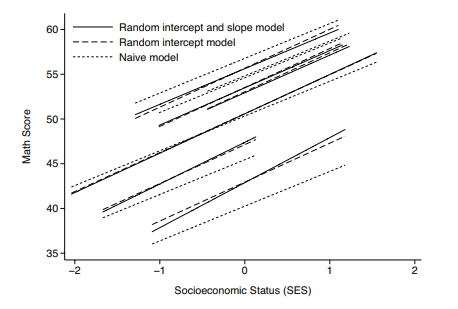
More complex models are possible. For example, we might think that the effect of SES on math scores is different for different schools. We can choose a model that allows each school to have its own SES slope. Because the effect of schools is considered a random effect, the SES slope would be a random effect as well as the intercept. In this case not only the intercept, but also the slope for SES is modeled at the school level and represents a second random effect called a random slope. The mathematical representation of this random intercept and random slope model is
$$
\begin{aligned}
\text { MathScore }{i j} &=\beta{0 j}+\beta_{1 j} \text { SES }{i j}+e{i j} \
\beta_{0 j} &=\gamma_{00}+\gamma_{01} \text { SchoolType }{j}+U{0 j} \
\beta_{1 j} &=\gamma_{10}+U_{1 j}
\end{aligned}
$$
where $\gamma_{10}$ represents an average slope across all schools and $U_{1 j}$ represents the value of the random effect (random slope) for school $j$ (which is expressed as the difference between the slope for school $j$ and the average slope across all schools). For this model, the combined equation becomes:
$$
\begin{aligned}
\text { MathScore }{i j}=& \gamma{00}+\gamma_{01} \text { SchoolType }{j}+\gamma{10} \mathrm{SES}{i j}+U{1 j} \mathrm{SES}{i j} \ &+U{0 j}+e_{i j}
\end{aligned}
$$
The term $U_{1 j}$ in the combined equation represents the random slope for SES.
If the effect of gender is added to the model and considered to be different for different schools, then the coefficient for gender could be conceptualized as a random effect as well and another equation added for such an effect $\beta_{2 j}$.
$$
\begin{aligned}
\text { MathScore }{i j} &=\beta{0 j}+\beta_{1 j} \text { SES }{i j}+\beta{2 j} \text { gender }{i j}+e{i j} \
\beta_{0 j} &=\gamma_{00}+\gamma_{01} \text { SchoolType }{j}+U{0 j} \
\beta_{1 j} &=\gamma_{10}+U_{1 j} \
\beta_{2 j} &=\gamma_{20}+U_{2 j}
\end{aligned}
$$

统计代写|多元统计分析作业代写Multivariate Statistical Analysis代考|Regression of clustered data with a binary outcome

Based on Figure 18.4, one might model the growth of the mice linearly. In the hierarchical model notation using subscript $i$ for observations made on different days and subscript $j$ for different mice and using a model with only a random intercept, this can be described as

CHAPTER 18. CORRELATED OUTCOMES REGRESSION
$$
\begin{aligned}
\text { Weight }{i j} &=\beta{0 j}+\beta_{1 j} \text { Day }{i}+e{i j} \
\beta_{0 j} &=\gamma_{00}+U_{0 j} \
\beta_{1 j} &=\gamma_{10}
\end{aligned}
$$
For the above model it is typically assumed that the $e_{i j}$ are normally distributed with mean zero. The weights of different mice (on the same or different days) are assumed to not be correlated, i.e., the correlation between $e_{i j}$ and $e_{i^{} j^{}}$ (where $j \neq j^{*}$ ) is zero. But the correlation between $e_{i j}$ and $e_{i} j$ (i.e., the correlation between different times of observation for the same mouse) is modeled according to one of the correlation matrices described above [AR(1), unstructured or exchangeable]. In other words, observations that lie on the same line in Figure $18.4$ are assumed to be correlated, but any observations from different lines are not.

As with the hierarchical models described in previous sections, the hierarchical nature of the data can easily become very complicated. In the case of the mice, data potentially could be correlated on a different level, e.g., if the mice came from different litters.

If we want to model not only the intercept, but also the slope, as random, then this can be formulated as:
$$
\begin{aligned}
\text { Weight }{i j} &=\beta{0 j}+\beta_{1 j} \text { Day }+e_{i j} \
\beta_{0 j} &=\gamma_{00}+U_{0 j} \
\beta_{1 j} &=\gamma_{10}+U_{1 j}
\end{aligned}
$$

假设检验代写

统计代写|多元统计分析作业代写Multivariate Statistical Analysis代考|Basic concepts

代表残差。该残差的定义方式与第 7 章中使用的定义类似，因为它是单个结果值（此处为数学分数）与模型预测值之间的差异。值得注意的是，SES 是一个派生的连续中心变量，它是根据父母的教育水平、父母双方的职业和家庭收入（值范围从−2.41到1.85; 如需更多信息，请访问附录 A) 中提到的网站。更一般地说，模型可以写成：
和一世=b0+b1X1一世+b2X2一世+和一世
请注意，在模型的上述公式中，下标一世学校数据集从 1 到 519 运行，其中包含 519 名学生。

同样，上述模型没有考虑数据的分层性质，即学生嵌套在学校内的事实。可以考虑将每所学校的指标变量添加到上述模型中。这样的模型可以写成
MathScore一世=b0+b1学校类型一世+b2他的一世
+b3( 学校 2)一世+…+b24( 学校 23)一世+和一世
其中 School 2 到 School 23 代表指示变量，如果学生取值为 1一世属于指定的学校。
或者更笼统地说
和一世=b0+b1X1一世+b2X2一世+b3X3一世+…+b24X24一世+和一世

统计代写|多元统计分析作业代写Multivariate Statistical Analysis代考|Regression of clustered data with a continuous outcomea

更复杂的模型是可能的。例如，我们可能认为不同学校的 SES 对数学成绩的影响是不同的。我们可以选择一个模型，让每所学校都有自己的 SES 斜率。因为学校的影响被认为是随机效应，所以 SES 斜率和截距一样都是随机效应。在这种情况下，不仅截距，而且 SES 的斜率都在学校级别建模，并表示称为随机斜率的第二种随机效应。这个随机截距和随机斜率模型的数学表示是
数学分数一世j=b0j+b1j 他的一世j+和一世j b0j=C00+C01 学校类型 j+ü0j b1j=C10+ü1j
在哪里C10代表所有学校的平均斜率，并且ü1j表示学校的随机效应（随机斜率）的值j（表示为学校斜率之间的差异j和所有学校的平均坡度）。对于该模型，组合方程变为：
数学分数一世j=C00+C01 学校类型 j+C10小号和小号一世j+ü1j小号和小号一世j +ü0j+和一世j
术语ü1j组合方程中的表示 SES 的随机斜率。
如果将性别效应添加到模型中并认为不同学校的影响不同，那么性别系数也可以概念化为随机效应，并为这种效应添加另一个方程b2j.
数学分数一世j=b0j+b1j 他的一世j+b2j 性别一世j+和一世j b0j=C00+C01 学校类型 j+ü0j b1j=C10+ü1j b2j=C20+ü2j

统计代写|多元统计分析作业代写Multivariate Statistical Analysis代考|Regression of clustered data with a binary outcome

根据图 18.4，可以对小鼠的生长进行线性建模。在使用下标的层次模型表示法中一世用于在不同日期和下标进行的观察j对于不同的小鼠并使用只有随机截距的模型，这可以描述为

第 18 章相关结果回归
重量一世j=b0j+b1j 日一世+和一世j b0j=C00+ü0j b1j=C10
对于上述模型，通常假设和一世j均值为零的正态分布。假设不同小鼠（同一天或不同天）的体重不相关，即和一世j和和一世j（在哪里j≠j∗) 为零。但是之间的相关性和一世j和和一世j（即，同一只小鼠的不同观察时间之间的相关性）根据上述相关矩阵之一建模[AR（1），非结构化或可交换]。换句话说，位于图 1 中同一条线上的观察18.4假设是相关的，但来自不同行的任何观察都不是。

与前几节中描述的层次模型一样，数据的层次性质很容易变得非常复杂。在老鼠的情况下，数据可能在不同的水平上相互关联，例如，如果老鼠来自不同的窝。

如果我们不仅要对截距建模，还要对斜率建模，作为随机的，那么这可以表述为：
重量一世j=b0j+b1j 日 +和一世j b0j=C00+ü0j b1j=C10+ü1j

统计代写| 广义线性模型project代写Generalized Linear Model代考|Binary Response请认准statistics-lab™

统计代写请认准statistics-lab™. statistics-lab™为您的留学生涯保驾护航。

随机过程代考

在概率论概念中，随机过程是随机变量的集合。若一随机系统的样本点是随机函数，则称此函数为样本函数，这一随机系统全部样本函数的集合是一个随机过程。实际应用中，样本函数的一般定义在时间域或者空间域。 随机过程的实例如股票和汇率的波动、语音信号、视频信号、体温的变化，随机运动如布朗运动、随机徘徊等等。

贝叶斯方法代考

贝叶斯统计概念及数据分析表示使用概率陈述回答有关未知参数的研究问题以及统计范式。后验分布包括关于参数的先验分布，和基于观测数据提供关于参数的信息似然模型。根据选择的先验分布和似然模型，后验分布可以解析或近似，例如，马尔科夫链蒙特卡罗 (MCMC) 方法之一。贝叶斯统计概念及数据分析使用后验分布来形成模型参数的各种摘要，包括点估计，如后验平均值、中位数、百分位数和称为可信区间的区间估计。此外，所有关于模型参数的统计检验都可以表示为基于估计后验分布的概率报表。

广义线性模型代考

广义线性模型（GLM）归属统计学领域，是一种应用灵活的线性回归模型。该模型允许因变量的偏差分布有除了正态分布之外的其它分布。

statistics-lab作为专业的留学生服务机构，多年来已为美国、英国、加拿大、澳洲等留学热门地的学生提供专业的学术服务，包括但不限于Essay代写，Assignment代写，Dissertation代写，Report代写，小组作业代写，Proposal代写，Paper代写，Presentation代写，计算机作业代写，论文修改和润色，网课代做，exam代考等等。写作范围涵盖高中，本科，研究生等海外留学全阶段，辐射金融，经济学，会计学，审计学，管理学等全球99%专业科目。写作团队既有专业英语母语作者，也有海外名校硕博留学生，每位写作老师都拥有过硬的语言能力，专业的学科背景和学术写作经验。我们承诺100%原创，100%专业，100%准时，100%满意。

机器学习代写

随着AI的大潮到来，Machine Learning逐渐成为一个新的学习热点。同时与传统CS相比，Machine Learning在其他领域也有着广泛的应用，因此这门学科成为不仅折磨CS专业同学的“小恶魔”，也是折磨生物、化学、统计等其他学科留学生的“大魔王”。学习Machine learning的一大绊脚石在于使用语言众多，跨学科范围广，所以学习起来尤其困难。但是不管你在学习Machine Learning时遇到任何难题，StudyGate专业导师团队都能为你轻松解决。

多元统计分析代考

基础数据: $N$ 个样本， $P$ 个变量数的单样本，组成的横列的数据表
变量定性: 分类和顺序；变量定量：数值
数学公式的角度分为: 因变量与自变量

时间序列分析代写

随机过程，是依赖于参数的一组随机变量的全体，参数通常是时间。随机变量是随机现象的数量表现，其时间序列是一组按照时间发生先后顺序进行排列的数据点序列。通常一组时间序列的时间间隔为一恒定值（如1秒，5分钟，12小时，7天，1年），因此时间序列可以作为离散时间数据进行分析处理。研究时间序列数据的意义在于现实中，往往需要研究某个事物其随时间发展变化的规律。这就需要通过研究该事物过去发展的历史记录，以得到其自身发展的规律。

回归分析代写

多元回归分析渐进（Multiple Regression Analysis Asymptotics）属于计量经济学领域，主要是一种数学上的统计分析方法，可以分析复杂情况下各影响因素的数学关系，在自然科学、社会和经济学等多个领域内应用广泛。

MATLAB代写

MATLAB 是一种用于技术计算的高性能语言。它将计算、可视化和编程集成在一个易于使用的环境中，其中问题和解决方案以熟悉的数学符号表示。典型用途包括：数学和计算算法开发建模、仿真和原型制作数据分析、探索和可视化科学和工程图形应用程序开发，包括图形用户界面构建MATLAB 是一个交互式系统，其基本数据元素是一个不需要维度的数组。这使您可以解决许多技术计算问题，尤其是那些具有矩阵和向量公式的问题，而只需用 C 或 Fortran 等标量非交互式语言编写程序所需的时间的一小部分。MATLAB 名称代表矩阵实验室。MATLAB 最初的编写目的是提供对由 LINPACK 和 EISPACK 项目开发的矩阵软件的轻松访问，这两个项目共同代表了矩阵计算软件的最新技术。MATLAB 经过多年的发展，得到了许多用户的投入。在大学环境中，它是数学、工程和科学入门和高级课程的标准教学工具。在工业领域，MATLAB 是高效研究、开发和分析的首选工具。MATLAB 具有一系列称为工具箱的特定于应用程序的解决方案。对于大多数 MATLAB 用户来说非常重要，工具箱允许您学习和应用专业技术。工具箱是 MATLAB 函数（M 文件）的综合集合，可扩展 MATLAB 环境以解决特定类别的问题。可用工具箱的领域包括信号处理、控制系统、神经网络、模糊逻辑、小波、仿真等。

统计代写|多元统计分析作业代写Multivariate Statistical Analysis代考|Log-linear analysisa

Posted on 2022年4月1日2022年4月1日 by statistics-lab

如果你也在怎样代写多元统计分析Multivariate Statistical Analysis这个学科遇到相关的难题，请随时右上角联系我们的24/7代写客服。

我们提供的多元统计分析Multivariate Statistical Analysis及其相关学科的代写，服务范围广, 其中包括但不限于:

Statistical Inference 统计推断
Statistical Computing 统计计算
Advanced Probability Theory 高等楖率论
Advanced Mathematical Statistics 高等数理统计学
(Generalized) Linear Models 广义线性模型
Statistical Machine Learning 统计机器学习
Longitudinal Data Analysis 纵向数据分析
Foundations of Data Science 数据科学基础

统计代写|多元统计分析作业代写Multivariate Statistical Analysis代考|Notation and sample considerations

The sample results given in Table $17.1$ were obtained from a single sample of size $N=294$ respondents. Table $17.4$ presents the usual notation for this case. Here $f_{11}$ (or 125 ) is the sample frequency in the first row (females) and column (low income) where the first subscript denotes the row and the second the column. The total for the first row is denoted by $f_{1+}$ (or 183 females) where the “t” in place of the column subscripts symbolizes that we added across the columns. The total for the first column is $f_{+1}$ and for the second column $f_{+2}$. The symbol $f_{i j}$ denotes the observed frequency in an arbitrary row $i$ and column $j$. For a three-way table three subscripts are needed with the third one denoting layer, four-way tables require four subscripts, etc.

If we divide the entire table by $N$ or $f_{++}$, then the resulting values will be the sample proportions denoted by $p_{i j}$ and the sample table of proportions is shown in Table 17.4. The proportion in the $i$ th row and $j$ th column is denoted by $p_{i j}$. The sample proportions are estimates of the population proportions that will be denoted by $\pi_{i j}$. The total sample proportion for the $i$ th row is denoted by

统计代写|多元统计分析作业代写Multivariate Statistical Analysis代考|Tests and models for two-way tables

In order to perform the chi-square test for a single sample, we need to calculate the expected frequencies under the null hypothesis of independence. The expected frequency is given by
$$
\mu_{i j}=N \pi_{i j}
$$
where the Greek letters denote population parameters, $i$ denotes the $i$ th row, and $j$ the $j$ th column. Theoretically, if two events are independent, then the probability of both of them occurring is the product of their individual probabilities. For example, the probability of obtaining two heads when you toss two fair coins is $(1 / 2)(1 / 2)=1 / 4$. If you multiply the probability of an event occurring by the number of trials, then you get the expected number of outcomes of that event. For example, if you toss two fair coins eight times, then the expected number of times in which you obtain two heads is $(8)(1 / 4)=2$ times.

Returning to two-way tables, the expected frequency in the $i j$ th cell when the null hypothesis of independence is true is given by
$$
\mu_{i j}=N \pi_{i+} \pi_{+j}
$$
where $\pi_{i+}$ denotes the marginal probability in the ith row and $\pi_{+j}$ denotes the marginal probability in the $j$ th column. In performing the test, sample proportions estimated from the margins of the table are used in place of the population parameters and their values are compared to the actual frequencies in the interior of the table using the chi-square statistic. For example, for Table 17.1, the expected value in the first cell is
$$
294(183 / 294)(179 / 294)=111.4
$$
which is then compared to the actual frequency of 125 . Here, more females have low income than we would have expected if income and gender were independent.

统计代写|多元统计分析作业代写Multivariate Statistical Analysis代考|Example of a two-way table

The log-linear model for the three-way table can be used to illustrate the different types of independence or lack of association that may exist in multiway tables. The simplest model is given by the complete independence (mutual independence) model. In order to demonstrate the models we will first redo Table $17.2$ in symbols so the correspondence between the symbols and the contents of the table will be clear. We have written Table $17.8$ in terms of the sample proportions that can be computed from a table such as Table $17.2$ by dividing the entries in the entire table by $N$. The marginal table given at the bottom is the sum of the top two-way tables (for layer $C=1$ plus for layer $C=2$ ). If we knew the true probabilities in the population, then the $p_{i j k}$ ‘s would be replaced by $\pi_{i j k}$ ‘s. Here $i$ denotes the $i$ th row, $j$ the $j$ th column, and $k$ the $k$ th layer and a ” $+”$ signifies a sum over that variable. Another marginal table of variable $A$ versus $C$ could be made using the column margins (column labelled Total) of the top two partial layer tables. A third marginal table for variables $B$ and $C$ can be made of the row marginals for the top two partial layer-tables; some programs can produce all of these tables by request.
Next we consider some special cases with and without associations.
Complete independence model
In this case, all variables are unassociated with each other. This is also called mutual independence. The probability in any cell $(i, j, k)$ is then given by
$$
\pi_{i j k}=\pi_{i++} \pi_{+j+} \pi_{++k}
$$
where $\pi_{i++}$ is the marginal probability for the $i$ th row (the lower marginal table row total), $\pi_{+j+}$ is the marginal probability for the $j$ th column (the lower marginal table column total), and $\pi_{++k}$ is the marginal probability for the $k$ th layer (the total for layer 1 and layer 2 tables). The sample estimates for the right side of the equation are $p_{i++}, p_{+j+}$, and $p_{++k}$, which can be found in Table $17.8$.
When complete independence holds, the three-way log-linear model is given by
$$
\log \mu_{i j k}=\lambda+\lambda_{A(i)}+\lambda_{B(j)}+\lambda_{C(k)}
$$
The model includes no parameters that signify an association.

假设检验代写

统计代写|多元统计分析作业代写Multivariate Statistical Analysis代考|Notation and sample considerations

表中给出的样品结果17.1从单个大小样本中获得ñ=294受访者。桌子17.4给出了这种情况下的常用符号。这里F11（或 125 ）是第一行（女性）和第一列（低收入）的样本频率，其中第一个下标表示行，第二个下标表示列。第一行的总数表示为F1+（或 183 位女性），其中“t”代替列下标表示我们在列中添加。第一列的总数是F+1对于第二列F+2. 符号F一世j表示在任意行中观察到的频率一世和列j. 对于三向表需要三个下标，第三个表示层，四向表需要四个下标，依此类推。

如果我们将整个表除以ñ要么F++，则结果值将是表示为的样本比例p一世j比例样本表见表17.4。中的比例一世第行和j第列表示为p一世j. 样本比例是对总体比例的估计，表示为圆周率一世j. 总样本比例一世第行表示为

统计代写|多元统计分析作业代写Multivariate Statistical Analysis代考|Tests and models for two-way tables

为了对单个样本进行卡方检验，我们需要计算独立零假设下的预期频率。预期频率由下式给出
μ一世j=ñ圆周率一世j
其中希腊字母表示人口参数，一世表示一世第行，和j这j第列。理论上，如果两个事件是独立的，那么它们发生的概率就是它们各自概率的乘积。例如，当你投掷两个公平硬币时获得两个正面的概率是(1/2)(1/2)=1/4. 如果您将事件发生的概率乘以试验次数，那么您将得到该事件的预期结果数。例如，如果您将两个公平的硬币抛八次，那么您获得两个正面的预期次数是(8)(1/4)=2次。

回到二维表，预期频率在一世j当独立性的零假设为真时，第 th 个单元格由下式给出
μ一世j=ñ圆周率一世+圆周率+j
在哪里圆周率一世+表示第 i 行的边际概率，并且圆周率+j表示边际概率j第列。在执行测试时，使用从表格边缘估计的样本比例代替总体参数，并使用卡方统计量将它们的值与表格内部的实际频率进行比较。例如，对于表 17.1，第一个单元格中的期望值为
294(183/294)(179/294)=111.4
然后将其与 125 的实际频率进行比较。在这里，如果收入和性别是独立的，那么低收入的女性比我们预期的要多。

统计代写|多元统计分析作业代写Multivariate Statistical Analysis代考|Example of a two-way table

三路表的对数线性模型可用于说明多路表中可能存在的不同类型的独立性或缺乏关联性。最简单的模型由完全独立（相互独立）模型给出。为了演示模型，我们将首先重做表17.2在符号中，因此符号与表格内容之间的对应关系将很清楚。我们写了表17.8根据可以从表格（例如 Table）计算的样本比例17.2通过将整个表中的条目除以ñ. 底部给出的边缘表是顶部双向表的总和（对于层C=1加层C=2）。如果我们知道总体中的真实概率，那么p一世j到的将被替换为圆周率一世j到的。这里一世表示一世扔，j这j第列，和到这到第层和一个”+”表示对该变量的总和。另一个边际变量表一种相对C可以使用顶部两个部分层表的列边距（标记为 Total 的列）来制作。变量的第三个边际表乙和C可以由顶部两个部分层表的行边缘组成；一些程序可以根据要求生成所有这些表。
接下来我们考虑一些有和没有关联的特殊情况。
完全独立模型
在这种情况下，所有变量都是不相关的。这也称为相互独立。任何单元格中的概率(一世,j,到)然后由
圆周率一世j到=圆周率一世++圆周率+j+圆周率++到
在哪里圆周率一世++是边际概率一世th 行（下边缘表行总计），圆周率+j+是边际概率jth 列（下边缘表列总计），以及圆周率++到是边际概率到th 层（第 1 层和第 2 层表的总和）。等式右侧的样本估计值为p一世++,p+j+，和p++到, 可以在表中找到17.8.
当完全独立成立时，三向对数线性模型由下式给出
日志⁡μ一世j到=λ+λ一种(一世)+λ乙(j)+λC(到)
该模型不包括表示关联的参数。

统计代写请认准statistics-lab™. statistics-lab™为您的留学生涯保驾护航。

随机过程代考

贝叶斯方法代考

广义线性模型代考

广义线性模型（GLM）归属统计学领域，是一种应用灵活的线性回归模型。该模型允许因变量的偏差分布有除了正态分布之外的其它分布。

机器学习代写

多元统计分析代考

基础数据: $N$ 个样本， $P$ 个变量数的单样本，组成的横列的数据表
变量定性: 分类和顺序；变量定量：数值
数学公式的角度分为: 因变量与自变量

时间序列分析代写

回归分析代写

MATLAB代写

统计代写|多元统计分析作业代写Multivariate Statistical Analysis代考|Cluster analysis

Posted on 2022年4月1日2022年4月1日 by statistics-lab

如果你也在怎样代写多元统计分析Multivariate Statistical Analysis这个学科遇到相关的难题，请随时右上角联系我们的24/7代写客服。

我们提供的多元统计分析Multivariate Statistical Analysis及其相关学科的代写，服务范围广, 其中包括但不限于:

Statistical Inference 统计推断
Statistical Computing 统计计算
Advanced Probability Theory 高等楖率论
Advanced Mathematical Statistics 高等数理统计学
(Generalized) Linear Models 广义线性模型
Statistical Machine Learning 统计机器学习
Longitudinal Data Analysis 纵向数据分析
Foundations of Data Science 数据科学基础

统计代写|多元统计分析作业代写Multivariate Statistical Analysis代考|Data example

A hypothetical data set was created to illustrate several of the concepts discussed in this chapter. Figure $16.2$ shows a plot of five observations for the two variables $X_{1}$ and $X_{2}$. This small data set will simplify the presentation since the analysis can be performed by hand.

Another data set we will use includes financial performance data from the January 1981 issue of Forbes. The variables used are those defined in Section 9.3. Table $16.1$ shows the data for 25 companies from three industries: chemical companies (the first 14 of the 31 discussed in Section 9.3), health care companies, and supermarket companies. The column labelled “Type” in Table $16.1$ lists the abbreviations Chem, Heal, and Groc for these three industries. In Section $16.6$ we will use two clustering techniques to group these companies and then check the agreement with their industrial type. These three industries were selected because they represent different stages of growth, different product lines, different management philosophies, different labor and capital requirements, etc. Among the chemical companies all of the large diversified firms were selected. From the major supermarket chains, the top six rated for return on equity were included. In the health care industry four of the five companies included were those connected with hospital management; the remaining company involves hospital supplies and equipment.

统计代写|多元统计分析作业代写Multivariate Statistical Analysis代考|Analytical clustering techniques

Hierarchical methods can be either agglomerative or divisive. In the agglomerative methods we begin with $N$ clusters, i.e., each observation constitutes its own cluster. In successive steps we combine the two closest clusters, thus reducing the number of clusters by one in each step. In the final step all observations are grouped into one cluster. In divisive methods we begin with one cluster containing all of the observations. In successive steps we split off the cases that are most dissimilar to the remaining ones. Most of the commonly used programs are of the agglomerative type, and we therefore do not discuss divisive methods further.

The centroid procedure is a widely used example of agglomerative methods. In the centroid method the distance between two clusters is defined as the distance between the group centroids (the centroid is the point whose coordinates are the means of all the observations in the cluster). If a cluster has one observation, then the centroid is the observation itself. The process proceeds by combining groups according to the distance between their centroids, the groups with the shortest distance being combined first.

The centroid method is illustrated in Figure $16.5$ for our hypothetical data. Initially, the closest two centroids (points) of the five hypothetical observations plotted in Figure $16.2$ are points 1 and 2 , so they are combined first and their centroid is obtained in step 1. In step 2, centroids (points) 3 and 4 are combined (and their centroid is obtained), since they are the closest now that points 1 and 2 have been replaced by their centroid. At step 3 the centroid of points 3 and 4 and centroid (point) 5 are combined, and the centroid is obtained. Finally, at the last step the centroid of points 1 and 2 and the centroid of points 3, 4, and 5 are combined to form a single group.

Figure $16.6$ illustrates the clustering steps based on the standardized hypothetical data. The results are identical to the previous ones, although this is not the case in general.

We could also have used the city-block distance. This distance is available by that name in many programs. As noted earlier in the discussion of distance measures, this distance can also be obtained from “power” measures.

Several other methods can be used to define the distance between two clusters. These are grouped in the computer programs under the heading of linkage methods. In these programs, the linkage distance is the distance between two clusters defined according to one of these methods.

统计代写|多元统计分析作业代写Multivariate Statistical Analysis代考|Cluster analysis for financial data set

In this section we apply some of the standard procedures to the financial performance data set shown in Table 16.1. In all our runs the data are first standardized as shown in Table 16.2. Recall that in
16.6. CLUSTER ANALYSIS FOR FINANCIAL DATA SET
329
cluster analysis the total sample is considered as a single sample. Thus the information on type of company is not used to derive the clusters. However, this information will be used to interpret the results of the various analyses.
Hierarchical clustering
The dendrogram or tree is shown in Figure 16.9. Default options including the centroid method with Euclidian distance were used with the standardized data. The horizontal axis lists the observation numbers in a particular order, which prevents the lines in the dendrogram from crossing each other. One result of this arrangement is that certain subgroups appearing near each other on the horizontal axis constitute clusters at various steps. Note that the distance is shown on the right vertical axis. These distances are measured being the centers of the two clusters just joined. On the left vertical axis the number of clusters is listed.

In Figure 16.9, companies 1,2, and 3 form a single cluster, with the grouping being completed when there are 22 clusters. Similarly, at the opposite end $15,16,18$, and 17 (all health care companies) form a single cluster at the step in which there are two clusters. Company 22 stays by itself until there are only four clusters.

假设检验代写

统计代写|多元统计分析作业代写Multivariate Statistical Analysis代考|Data example

创建了一个假设的数据集来说明本章讨论的几个概念。数字16.2显示两个变量的五个观测值的图X1和X2. 这个小数据集将简化演示，因为可以手动执行分析。

我们将使用的另一个数据集包括 1981 年 1 月版《福布斯》的财务业绩数据。使用的变量是第 9.3 节中定义的变量。桌子16.1显示来自三个行业的 25 家公司的数据：化工公司（第 9.3 节讨论的 31 家公司中的前 14 家）、医疗保健公司和超市公司。表中标有“类型”的列16.1列出了这三个行业的缩写 Chem、Heal 和 Groc。在部分16.6我们将使用两种聚类技术对这些公司进行分组，然后检查与它们的行业类型的一致性。之所以选择这三个行业，是因为它们代表了不同的成长阶段、不同的产品线、不同的管理理念、不同的劳动力和资本需求等。在化工公司中，所有大型多元化公司都被选中。在主要的连锁超市中，股本回报率排名前六位。在医疗保健行业，五家公司中有四家是与医院管理相关的公司；其余公司涉及医院用品和设备。

统计代写|多元统计分析作业代写Multivariate Statistical Analysis代考|Analytical clustering techniques

分层方法可以是凝聚的或分裂的。在我们开始的凝聚方法中ñ集群，即每个观察都构成自己的集群。在连续的步骤中，我们将两个最接近的集群组合在一起，从而在每一步中将集群的数量减少一个。在最后一步中，所有观察都被分组到一个集群中。在分裂方法中，我们从一个包含所有观察值的集群开始。在连续的步骤中，我们将与其余案例最不同的案例分开。大多数常用的程序都是凝聚型的，因此我们不进一步讨论分裂的方法。

质心过程是一个广泛使用的凝聚方法的例子。在质心方法中，两个聚类之间的距离定义为组质心之间的距离（质心是其坐标是聚类中所有观测值的平均值的点）。如果一个集群有一个观测值，那么质心就是观测值本身。该过程通过根据质心之间的距离组合组来进行，首先组合具有最短距离的组。

质心法如图16.5对于我们的假设数据。最初，图中绘制的五个假设观测值中最接近的两个质心（点）16.2是点 1 和 2 ，因此首先将它们组合在一起，并在步骤 1 中获得它们的质心。在步骤 2 中，将质心（点）3 和 4 组合起来（并获得它们的质心），因为它们现在最接近点 1和 2 已被其质心取代。在步骤 3 中，将点 3 和 4 的质心与质心（点）5 合并，得到质心。最后，在最后一步将点 1 和 2 的质心与点 3、4 和 5 的质心组合成一个组。

数字16.6说明了基于标准化假设数据的聚类步骤。结果与之前的结果相同，尽管通常情况并非如此。

我们也可以使用城市街区距离。该距离在许多程序中都可以通过该名称获得。正如前面对距离测量的讨论所指出的，这个距离也可以从“功率”测量中获得。

可以使用其他几种方法来定义两个集群之间的距离。这些在链接方法标题下的计算机程序中分组。在这些程序中，链接距离是根据这些方法之一定义的两个集群之间的距离。

统计代写|多元统计分析作业代写Multivariate Statistical Analysis代考|Cluster analysis for financial data set

在本节中，我们将一些标准程序应用于表 16.1 所示的财务绩效数据集。在我们所有的运行中，首先对数据进行标准化，如表 16.2 所示。回想一下
16.6 中的内容。财务数据集的聚类分析
329
聚类分析总样本被视为单个样本。因此，关于公司类型的信息不用于派生集群。但是，此信息将用于解释各种分析的结果。
层次聚类
树状图或树如图 16.9 所示。默认选项包括具有欧几里得距离的质心方法与标准化数据一起使用。水平轴按特定顺序列出观察编号，这可以防止树状图中的线条相互交叉。这种安排的一个结果是，在水平轴上彼此靠近的某些子组在各个步骤中构成了集群。请注意，距离显示在右侧垂直轴上。这些距离被测量为刚刚加入的两个集群的中心。在左侧垂直轴上列出了集群的数量。

在图 16.9 中，公司 1、2 和 3 形成一个集群，当集群有 22 个时，分组就完成了。同样，在另一端15,16,18，和 17 家（所有医疗保健公司）在有两个集群的步骤中形成一个集群。公司 22 一直保持独立，直到只有四个集群。

统计代写请认准statistics-lab™. statistics-lab™为您的留学生涯保驾护航。

随机过程代考

贝叶斯方法代考

广义线性模型代考

广义线性模型（GLM）归属统计学领域，是一种应用灵活的线性回归模型。该模型允许因变量的偏差分布有除了正态分布之外的其它分布。

机器学习代写

多元统计分析代考

基础数据: $N$ 个样本， $P$ 个变量数的单样本，组成的横列的数据表
变量定性: 分类和顺序；变量定量：数值
数学公式的角度分为: 因变量与自变量

时间序列分析代写

回归分析代写

MATLAB代写

统计代写|多元统计分析作业代写Multivariate Statistical Analysis代考|Factor analysis

Posted on 2022年4月1日2022年4月1日 by statistics-lab

如果你也在怎样代写多元统计分析Multivariate Statistical Analysis这个学科遇到相关的难题，请随时右上角联系我们的24/7代写客服。

我们提供的多元统计分析Multivariate Statistical Analysis及其相关学科的代写，服务范围广, 其中包括但不限于:

Statistical Inference 统计推断
Statistical Computing 统计计算
Advanced Probability Theory 高等楖率论
Advanced Mathematical Statistics 高等数理统计学
(Generalized) Linear Models 广义线性模型
Statistical Machine Learning 统计机器学习
Longitudinal Data Analysis 纵向数据分析
Foundations of Data Science 数据科学基础

统计代写|多元统计分析作业代写Multivariate Statistical Analysis代考|Data example

where the following assumptions are made:

$m$ is the number of common factors (typically this number is much smaller than $P$ ),
$F_{1}, F_{2}, \ldots, F_{m}$ are the common factors. These factors are assumed to have zero means and unit variances.
$I_{i j}$ is the coefficient of $F_{j}$ in the linear combination describing $x_{i}$. This term is called the loading of the $i$ th variable on the $j$ th common factor.
$e_{1}, e_{2}, \ldots, e_{P}$ are unique factors, each relating to one of the original variables.
The above equations and assumptions constitute the factor model. Thus, each of the response variables is composed of a part due to the common factors and a part due to its own unique factor. The part due to the common factors is assumed to be a linear combination of these factors.

As an example, suppose that $x_{1}, x_{2}, x_{3}, x_{4}, x_{5}$ are the standardized scores of an individual on five tests. If $m=2$, we assume the following model:
$$
\begin{aligned}
x_{1} &=l_{11} F_{1}+l_{12} F_{2}+e_{1} \
x_{2} &=l_{21} F_{1}+l_{22} F_{2}+e_{2} \
& \vdots \
x_{5} &=l_{51} F_{1}+l_{52} F_{2}+e_{5}
\end{aligned}
$$

统计代写|多元统计分析作业代写Multivariate Statistical Analysis代考|Initial extraction: principal components

In this section and the next we discuss two methods for the initial extraction of common factors. We begin with the principal components analysis method, which can be found in most of the standard factor analysis programs. The basic idea is to choose the first $m$ principal components and modify them to fit the factor model defined in the previous section. The reason for choosing the first $m$ principal components, rather than any others, is that they explain the greatest proportion of the variance and are therefore the most important. Note that the principal components are also uncorrelated and thus present an attractive choice as factors.

To satisfy the assumption of unit variances of the factors, we divide each principal component by its standard deviation. That is, we define the $j$ th common factor $F_{j}$ as $F_{j}=C_{j} /\left(\operatorname{Var} C_{j}\right)^{1 / 2}$, where $C_{j}$ is the $j$ th principal component.

To express each variable $x_{i}$ in terms of the $F_{j}$ ‘s, we first recall the relationship between the variables $x_{i}$ and the principal components $C_{j}$. Specifically,
$$
\begin{aligned}
C_{1} &=a_{11} x_{1}+a_{12} x_{2}+\cdots+a_{1 P} x_{P} \
C_{2} &=a_{21} x_{1}+a_{22} x_{2}+\cdots+a_{2 P} x_{P} \
& \vdots \
C_{P} &=a_{P 1} x_{1}+a_{P 2} x_{2}+\cdots+a_{P P} x_{P}
\end{aligned}
$$
It may be shown mathematically that this set of equations can be inverted to express the $x_{i}$ ‘s as functions of the $C_{j}$ ‘s. The result is:
$$
\begin{aligned}
x_{1} &=a_{11} C_{1}+a_{21} C_{2}+\cdots+a_{P 1} C_{P} \
x_{2} &=a_{12} C_{1}+a_{22} C_{2}+\cdots+a_{P 2} C_{P} \
& \vdots \
x_{P} &=a_{1 P} C_{1}+a_{2 P} C_{2}+\cdots+a_{P P} C_{P}
\end{aligned}
$$
Note that the rows of the first set of equations become the columns of the second set of equations.
Now since $F_{j}=C_{j} /\left(\operatorname{Var} C_{j}\right)^{1 / 2}$, it follows that $C_{j}=F_{j}\left(\operatorname{Var} C_{j}\right)^{1 / 2}$, and we can then express the $i$ th equation as
$$
x_{1}=a_{1 i} F_{1}\left(\operatorname{Var} C_{1}\right)^{1 / 2}+a_{2 i} F_{2}\left(\operatorname{Var} C_{2}\right)^{1 / 2}+\cdots+a_{P i} F_{P}\left(\operatorname{Var} C_{P}\right)^{1 / 2}
$$
This last equation is now modified in two ways.

统计代写|多元统计分析作业代写Multivariate Statistical Analysis代考|Initial extraction: iterated componentsa

The second method of extracting initial factors is a modification of the principal components analysis method. It has different names in different packages. It is called principal factor analysis or principal axis factoring approach in many texts.

To understand this method, you should recall that the communality is the part of the variance of each variable associated with the common factors. The principle underlying the iterated solution states that we should perform the factor analysis by using the communalities in place of the original variance. This principle entails substituting communality estimates for the l’s representing the variances of the standardized variables along the diagonal of the correlation matrix. With 1 ‘s in the diagonal we are factoring the total variance of the variables; with communalities in the diagonal we are factoring the variance associated with the common factors. Thus with communalities along the diagonal we select those common factors that maximize the total communality.

Many factor analysts consider maximizing the total communality a more attractive objective than maximizing the total proportion of the explained variance, as is done in the principal components method. The problem is that communalities are not known before the factor analysis is performed. Some initial estimates of the communalities must be obtained prior to the analysis. Various procedures exist, and we recommend, in the absence of a prior estimates, that the investigator use the default option in the particular program since the resulting factor solution is usually little affected by the initial communality estimates.

The steps performed by a packaged program in carrying out the iterated factor extraction are summarized as follows:

Find the initial communality estimates.
Substitute the communalities for the diagonal elements (1’s) in the correlation matrix.
Extract $m$ principal components from the modified matrix.
Multiply the principal components coefficients by the standard deviation of the respective principal components to obtain factor loadings.
Compute new communalities from the computed factor loadings.
Replace the communalities in step 2 with these new communalities and repeat steps 3,4 , and 5 . This step constitutes an iteration.
Continue iterating, stopping when the communalities stay essentially the same in the last two iterations.

假设检验代写

统计代写|多元统计分析作业代写Multivariate Statistical Analysis代考|Data example

作出以下假设：

米是公因子的个数（通常这个数字远小于磷),
F1,F2,…,F米是共同因素。假设这些因素的均值和单位方差为零。
一世一世j是系数Fj在线性组合描述X一世. 这个术语被称为加载一世上的变量j公因数。
和1,和2,…,和磷是独特的因素，每个因素都与原始变量之一有关。
上述方程和假设构成了因子模型。因此，每个响应变量都由共同因素的一部分和自身独特因素的一部分组成。假设因公因子而产生的部分是这些因子的线性组合。

例如，假设X1,X2,X3,X4,X5是个人在五项测试中的标准化分数。如果米=2，我们假设以下模型：
X1=一世11F1+一世12F2+和1 X2=一世21F1+一世22F2+和2 ⋮ X5=一世51F1+一世52F2+和5

统计代写|多元统计分析作业代写Multivariate Statistical Analysis代考|Initial extraction: principal components

在本节和下一节中，我们将讨论两种初始提取公因子的方法。我们从主成分分析方法开始，它可以在大多数标准因子分析程序中找到。基本思路是选择第一个米主成分并对其进行修改以适应上一节中定义的因子模型。选择第一的理由米主成分，而不是任何其他成分，是它们解释了最大比例的方差，因此是最重要的。请注意，主成分也是不相关的，因此作为因子是一个有吸引力的选择。

为了满足因子单位方差的假设，我们将每个主成分除以其标准差。也就是说，我们定义j公因数Fj作为Fj=Cj/(在哪里⁡Cj)1/2，在哪里Cj是个j主成分。

表达每个变量X一世方面Fj的，我们先回忆一下变量之间的关系X一世和主要成分Cj. 具体来说，
C1=一种11X1+一种12X2+⋯+一种1磷X磷 C2=一种21X1+一种22X2+⋯+一种2磷X磷 ⋮ C磷=一种磷1X1+一种磷2X2+⋯+一种磷磷X磷
从数学上可以看出，这组方程可以倒置来表达X一世的作为函数Cj的。结果是：
X1=一种11C1+一种21C2+⋯+一种磷1C磷 X2=一种12C1+一种22C2+⋯+一种磷2C磷 ⋮ X磷=一种1磷C1+一种2磷C2+⋯+一种磷磷C磷
请注意，第一组方程的行变成了第二组方程的列。
现在自从Fj=Cj/(在哪里⁡Cj)1/2，它遵循Cj=Fj(在哪里⁡Cj)1/2，然后我们可以表达一世方程为
X1=一种1一世F1(在哪里⁡C1)1/2+一种2一世F2(在哪里⁡C2)1/2+⋯+一种磷一世F磷(在哪里⁡C磷)1/2
现在以两种方式修改最后一个方程。

统计代写|多元统计分析作业代写Multivariate Statistical Analysis代考|Initial extraction: iterated componentsa

第二种提取初始因子的方法是对主成分分析法的改进。它在不同的包中有不同的名称。在许多文本中称为主因子分析或主轴因子分解方法。

要理解这种方法，您应该记得，公共性是与公共因素相关的每个变量的方差的一部分。迭代解决方案的基本原理表明，我们应该通过使用公共性代替原始方差来执行因子分析。该原则需要用公共估计值代替表示沿相关矩阵对角线的标准化变量的方差的 l。对角线中有 1 ，我们正在考虑变量的总方差；对于对角线中的公用性，我们正在考虑与公用因子相关的方差。因此，对于沿对角线的公共性，我们选择那些使总公共性最大化的公共因素。

许多因子分析师认为最大化总公共性比最大化解释方差的总比例更有吸引力，就像在主成分方法中所做的那样。问题是在进行因子分析之前社区是未知的。必须在分析之前获得对社区的一些初步估计。存在各种程序，我们建议，在没有事先估计的情况下，调查人员在特定程序中使用默认选项，因为得到的因子解通常很少受到初始公共估计的影响。

打包程序执行迭代因子提取的步骤总结如下：

找到最初的社区估计。
用相关矩阵中的对角元素 (1) 替换公有性。
提炼米来自修改矩阵的主成分。
将主成分系数乘以各个主成分的标准差以获得因子载荷。
根据计算的因子载荷计算新的社区。
将步骤 2 中的社区替换为这些新社区，然后重复步骤 3、4 和 5。这一步构成一个迭代。
继续迭代，当社区在最后两次迭代中基本保持不变时停止。

统计代写请认准statistics-lab™. statistics-lab™为您的留学生涯保驾护航。

随机过程代考

贝叶斯方法代考

广义线性模型代考

广义线性模型（GLM）归属统计学领域，是一种应用灵活的线性回归模型。该模型允许因变量的偏差分布有除了正态分布之外的其它分布。

机器学习代写

多元统计分析代考

基础数据: $N$ 个样本， $P$ 个变量数的单样本，组成的横列的数据表
变量定性: 分类和顺序；变量定量：数值
数学公式的角度分为: 因变量与自变量

时间序列分析代写

回归分析代写

MATLAB代写

统计代写|多元统计分析作业代写Multivariate Statistical Analysis代考|Principal components analysis

Posted on 2022年4月1日2022年4月1日 by statistics-lab

如果你也在怎样代写多元统计分析Multivariate Statistical Analysis这个学科遇到相关的难题，请随时右上角联系我们的24/7代写客服。

我们提供的多元统计分析Multivariate Statistical Analysis及其相关学科的代写，服务范围广, 其中包括但不限于:

Statistical Inference 统计推断
Statistical Computing 统计计算
Advanced Probability Theory 高等楖率论
Advanced Mathematical Statistics 高等数理统计学
(Generalized) Linear Models 广义线性模型
Statistical Machine Learning 统计机器学习
Longitudinal Data Analysis 纵向数据分析
Foundations of Data Science 数据科学基础

统计代写|多元统计分析作业代写Multivariate Statistical Analysis代考|When is principal components analysis used?

Principal components analysis is performed in order to simplify the description of a set of interrelated variables. In principal components analysis the variables are treated equally; i.e., they are not divided into dependent and independent variables, as in regression analysis.

The technique can be summarized as a method of transforming the original variables into new, uncorrelated variables. The new variables are called the principal components. Each principal component is a linear combination of the original variables. One measure of the amount of information conveyed by each principal component is its variance. For this reason the principal components are arranged in order of decreasing variance. Thus the most informative principal component is the first, and the least informative is the last (a variable with zero variance does not distinguish between the members of the population).

An investigator may wish to reduce the dimensionality of the problem, i.e., reduce the number of variables without losing much of the information. This objective can be achieved by choosing to analyze only the first few principal components. The principal components not analyzed convey only a small amount of information since their variances are small. This technique is attractive for another reason, namely, that the principal components are not intercorrelated. Thus instead of analyzing a large number of original variables with complex interrelationships, the investigator can analyze a small number of uncorrelated principal components.

The selected principal components may also be used to test for their normality. If the principal components are not normally distributed, then neither are the original variables. Another use of the principal components is to search for outliers. A histogram of each of the principal components can identify those individuals with very large or very small values; these values are candidates for outliers or blunders.

In regression analysis it is sometimes useful to obtain the first few principal components corresponding to the $X$ variables and then perform the regression on the selected components. This tactic is useful for overcoming the problem of multicollinearity since the principal components are uncorrelated (Chatterjee and Hadi, 2012). Principal components analysis can also be viewed as a step toward factor analysis (Chapter 15).

统计代写|多元统计分析作业代写Multivariate Statistical Analysis代考|Data example

Suppose that we have a random sample of $N$ observations on $X_{1}$ and $X_{2}$. For ease of interpretation we subtract the sample mean from each observation, thus obtaining
$$
x_{1}=X_{1}-\bar{X}{1} $$ and $$ x{2}=X_{2}-X_{2}
$$
Note that this technique makes the means of $x_{1}$ and $x_{2}$ equal to zero but does not alter the sample variances $S_{1}^{2}$ and $S_{2}^{2}$ or the correlation $r$.

The basic idea is to create two new variables, $C_{1}$ and $C_{2}$, called the principal components. These new variables are linear functions of $x_{1}$ and $x_{2}$ and can therefore be written as
$$
\begin{aligned}
&C_{1}=a_{11} x_{1}+a_{12} x_{2} \
&C_{2}=a_{21} x_{1}+a_{22} x_{2}
\end{aligned}
$$
We note that for any set of values of the coefficients $a_{11}, a_{12}, a_{21}, a_{22}$, we can introduce the $N$ observed $x_{1}$ and $x_{2}$ and obtain $N$ values of $C_{1}$ and $C_{2}$. The means and variances of the $N$ values of $C_{1}$ and $C_{2}$ are
$$
\begin{aligned}
\text { mean } C_{1} &=\text { mean } C_{2}=0 \
\operatorname{Var} C_{1} &=a_{11}^{2} S_{1}^{2}+a_{12}^{2} S_{2}^{2}+2 a_{11} a_{12} r S_{1} S_{2} \
\operatorname{Var} C_{2} &=a_{21}^{2} S_{1}^{2}+a_{22}^{2} S_{2}^{2}+2 a_{21} a_{22} r S_{1} S_{2}
\end{aligned}
$$
where $S_{i}^{2}=\operatorname{Var} X_{i}$

统计代写|多元统计分析作业代写Multivariate Statistical Analysis代考|Interpretation

Transforming coefficients to correlations
To interpret the meaning of the first principal component, we recall that it was expressed as
$$
C_{1}=0.851 x_{1}+0.525 x_{2}
$$
The coefficient $0.851$ can be transformed into a correlation between $x_{1}$ and $C_{1}$. In general, the correlation between the $i$ th principal component and the $j$ th $x$ variable is
$$
r_{i j}=\frac{a_{i j}\left(\operatorname{Var} C_{i}\right)^{1 / 2}}{\left(\operatorname{Var} x_{j}\right)^{1 / 2}}
$$
where $a_{i j}$ is the coefficient of $x_{j}$ for the ith principal component. For example, the correlation between $C_{1}$ and $x_{1}$ is
$$
r_{11}=\frac{0.85(135.04)^{1 / 2}}{(103.98)^{1 / 2}}=0.969
$$
and the correlation between $C_{1}$ and $x_{2}$ is
$$
r_{12}=\frac{0.525(135.04)^{1 / 2}}{(53.51)^{1 / 2}}=0.834
$$
Note that both of these correlations are fairly high and positive. As can be seen from Figure 14.3, when either $x_{1}$ or $x_{2}$ increases, so will $C_{1}$. This result occurs often in principal components analysis whereby the first component is positively correlated with all of the original variables.

假设检验代写

统计代写|多元统计分析作业代写Multivariate Statistical Analysis代考|When is principal components analysis used?

进行主成分分析是为了简化一组相互关联的变量的描述。在主成分分析中，变量被平等对待；即，它们不像回归分析那样分为因变量和自变量。

该技术可以概括为一种将原始变量转换为新的、不相关的变量的方法。新变量称为主成分。每个主成分都是原始变量的线性组合。每个主成分传达的信息量的一个衡量标准是它的方差。因此，主成分按方差递减的顺序排列。因此，信息最多的主成分是第一个，而信息最少的是最后一个（方差为零的变量不区分总体成员）。

调查人员可能希望减少问题的维数，即减少变量的数量而不丢失很多信息。这个目标可以通过选择只分析前几个主成分来实现。未分析的主成分仅传达少量信息，因为它们的方差很小。这种技术之所以有吸引力是因为另一个原因，即主成分不相关。因此，调查者可以分析少量不相关的主成分，而不是分析大量具有复杂相互关系的原始变量。

选定的主成分也可用于检验它们的正态性。如果主成分不是正态分布的，那么原始变量也不是。主成分的另一个用途是搜索异常值。每个主成分的直方图可以识别具有非常大或非常小的值的个体；这些值是异常值或错误的候选值。

在回归分析中，有时获得对应于X变量，然后对选定的组件执行回归。这种策略对于克服多重共线性问题很有用，因为主成分是不相关的（Chatterjee 和 Hadi，2012 年）。主成分分析也可以看作是因子分析的一个步骤（第 15 章）。

统计代写|多元统计分析作业代写Multivariate Statistical Analysis代考|Data example

假设我们有一个随机样本ñ意见X1和X2. 为了便于解释，我们从每个观察中减去样本均值，从而获得
X1=X1−X¯1和X2=X2−X2
请注意，这种技术使X1和X2等于零但不改变样本方差小号12和小号22或相关性r.

基本思想是创建两个新变量，C1和C2，称为主成分。这些新变量是X1和X2因此可以写成
C1=一种11X1+一种12X2 C2=一种21X1+一种22X2
我们注意到，对于任何一组系数值一种11,一种12,一种21,一种22，我们可以引入ñ观察到的X1和X2并获得ñ的值C1和C2. 均值和方差ñ的值C1和C2是
意思是 C1= 意思是 C2=0 在哪里⁡C1=一种112小号12+一种122小号22+2一种11一种12r小号1小号2 在哪里⁡C2=一种212小号12+一种222小号22+2一种21一种22r小号1小号2
在哪里小号一世2=在哪里⁡X一世

统计代写|多元统计分析作业代写Multivariate Statistical Analysis代考|Interpretation

将系数转换为相关性
为了解释第一个主成分的含义，我们记得它被表示为
C1=0.851X1+0.525X2
系数0.851可以转化为相关性X1和C1. 一般来说，两者之间的相关性一世主成分和jthX变量是
r一世j=一种一世j(在哪里⁡C一世)1/2(在哪里⁡Xj)1/2
在哪里一种一世j是系数Xj为第 i 个主成分。例如，之间的相关性C1和X1是
r11=0.85(135.04)1/2(103.98)1/2=0.969
以及之间的相关性C1和X2是
r12=0.525(135.04)1/2(53.51)1/2=0.834
请注意，这两种相关性都相当高且为正。从图 14.3 可以看出，当X1要么X2增加，所以会C1. 这个结果经常出现在主成分分析中，其中第一个成分与所有原始变量正相关。

统计代写请认准statistics-lab™. statistics-lab™为您的留学生涯保驾护航。

随机过程代考

贝叶斯方法代考

广义线性模型代考

广义线性模型（GLM）归属统计学领域，是一种应用灵活的线性回归模型。该模型允许因变量的偏差分布有除了正态分布之外的其它分布。

机器学习代写

多元统计分析代考

基础数据: $N$ 个样本， $P$ 个变量数的单样本，组成的横列的数据表
变量定性: 分类和顺序；变量定量：数值
数学公式的角度分为: 因变量与自变量

时间序列分析代写

回归分析代写

MATLAB代写

统计代写|多元统计分析作业代写Multivariate Statistical Analysis代考|Regression analysis with survival data

Posted on 2022年4月1日2022年4月1日 by statistics-lab

如果你也在怎样代写多元统计分析Multivariate Statistical Analysis这个学科遇到相关的难题，请随时右上角联系我们的24/7代写客服。

我们提供的多元统计分析Multivariate Statistical Analysis及其相关学科的代写，服务范围广, 其中包括但不限于:

Statistical Inference 统计推断
Statistical Computing 统计计算
Advanced Probability Theory 高等楖率论
Advanced Mathematical Statistics 高等数理统计学
(Generalized) Linear Models 广义线性模型
Statistical Machine Learning 统计机器学习
Longitudinal Data Analysis 纵向数据分析
Foundations of Data Science 数据科学基础

统计代写|多元统计分析作业代写Multivariate Statistical Analysis代考|Chapter outline

Survival analysis can be used to analyze data on the length of time it takes for a specific event to occur. This technique takes on different names, depending on the particular application on hand. For example, if the event under consideration is the death of a person, animal, or plant, then the name survival analysis is used. If the event is the failure of a manufactured item, e.g., a light bulb, then one speaks of failure time analysis or reliability theory (Smith, 2002). The term event history analysis is used by social scientists to describe applications in their fields (Yamaguchi, 1991). For example, analysis of the length of time it takes an employee to retire or resign from a given job could be called event history analysis. In this chapter, we will use the term survival analysis to mean any of the analyses just mentioned.

Survival analysis is a way of describing the distribution of the length of time to a given event. Suppose the event is termination of employment. We could simply draw a histogram of the length of time individuals are employed. Alternatively, we could use log length of employment as a dependent
255
256
CHAPTER 13. REGRESSION ANALYSIS WITH SURVIVAL DATA
variable and determine if it can be predicted by variables such as age, gender, educational level, or type of position (this will be discussed in Section 13.7). Another possibility would be to use the Cox regression model as described in Section 13.8.

Readers interested in a comprehensive coverage of the subject of survival analysis are advised to study one of the texts referenced in this chapter. In this chapter, our objective is to describe regression-type techniques that allow the user to examine the relationship between length of survival and a set of explanatory variables. The explanatory variables, often called covariates, can be either continuous, such as age or income, or they can be discrete, such as dummy variables that denote a treatment group. The material in Sections $13.3-13.5$ is intended as a summary of the background necessary to understand the remainder of the chapter.

统计代写|多元统计分析作业代写Multivariate Statistical Analysis代考|Common survival distributionsa

The simplest model for survival analysis assumes that the hazard function is constant over time, that is, $h(t)=\lambda$, where $\lambda$ is any constant greater than zero. This results in the exponential death density $f(t)=\lambda \exp (-\lambda t)$ and the exponential survival function $S(t)=\exp (-\lambda t)$. Graphically, the hazard function and the death density function are displayed in part (a) of Figure $13.7$ and Figure 13.8. This model assumes that having survived up to a given point in time has no effect on the probability of dying in the next instant. Although simple, this model has been successful in describing many phenomena observed in real life. For example, it has been demonstrated that the exponential distribution closely describes the length of time from the first to the second myocardial infarction in humans and the time from diagnosis to death for some cancers. The exponential distribution can be easily recognized from a flat (constant) hazard function plot. Such plots are available in the output of many software programs, as we will discuss in Section 13.10.

If the hazard function is not constant, the Weibull distribution should be considered. For this distribution, the hazard function may be expressed as $h(t)=\alpha \lambda(\lambda t)^{\alpha-1}$. The expressions for the density function, the cumulative distribution function, and the survival function can be found in specialized texts, e.g., Kalbfleisch and Prentice (2002). Figures 13.7b and $13.8 \mathrm{~b}$ show plots of the hazard and density functions for $\lambda=1$ and $\alpha=0.5,1.5$, and $2.5$. The value of $\alpha$ determines the shape of the distribution and for that reason it is called the shape parameter or index. Furthermore, as may be seen in Figure $13.7 \mathrm{~b}$, the value of $\alpha$ determines whether the hazard function increases or decreases over time. Namely, when $\alpha<1$ the hazard function is decreasing and when $\alpha>1$ it is increasing. When $\alpha=1$ the hazard is constant, and the Weibull and exponential distributions are identical. In that case, the exponential distribution is used. The value of $\lambda$ determines how much the distribution is stretched, and therefore it is called the scale parameter.

The Weibull distribution is used extensively in practice. Section $13.7$ describes a model in which this distribution is assumed. However, the reader should note that other distributions are sometimes used. These include the log-normal, gamma, and others (e.g., Kalbfleisch and Prentice, 2002 or Andersen et al., 1993).

A good way for deciding whether or not the Weibull distribution fits a set of data is to obtain a plot of $\log (-\log S(t))$ versus log time, and check whether the graph approximates a straight line (Section 13.10). If it does, then the Weibull distribution is appropriate and the methods described in Section $13.7$ can be used. If not, either another distribution may be assumed or the method described in Section $13.8$ can be used.a

统计代写|多元统计分析作业代写Multivariate Statistical Analysis代考|The log-linear regression model

In this section, we describe the use of multiple linear regression to study the relationship between survival time and a set of explanatory variables. Suppose that $t$ is survival time and $X_{1}, X_{2}, \ldots, X_{P}$ are the independent or explanatory variables. Let $Y=\log (t)$ be the dependent variable, where natural logarithms are used. Then the model assumes a linear relationship between $\log (t)$ and the $X$ ‘s. The model equation is
$$
\log (t)=\alpha+\beta_{1} X_{1}+\beta_{2} X_{2}+\cdots+\beta_{P} X_{P}+e
$$
where $e$ is an error term. This model is known as the log-linear regression model since the log of survival time is a linear function of the $X$ ‘s. If the distribution of $\log (t)$ were normal and if no censored observations exist in the data set, it would be possible to use the regression methods described
13.7. THE LOG-LINEAR REGRESSION MODEL
265
in Chapter 8 to analyze the data. However, in most practical situations some of the observations are censored, as was described in Section 13.3. Furthermore, $\log (t)$ is usually not normally distributed ( $t$ is often assumed to have a Weibull distribution). For those reasons, the method of maximum likelihood is used to obtain estimates of $\beta_{i}$ ‘s and their standard errors. When the Weibull distribution is assumed, the log-linear model is sometimes known as the accelerated life or accelerated failure time model (Kalbfleisch and Prentice, 2002).

假设检验代写

统计代写|多元统计分析作业代写Multivariate Statistical Analysis代考|Chapter outline

生存分析可用于分析特定事件发生所需时间长度的数据。这种技术有不同的名称，具体取决于手头的特定应用程序。例如，如果考虑的事件是人、动物或植物的死亡，则使用名称生存分析。如果事件是一个制造项目的故障，例如，一个灯泡，那么人们谈到故障时间分析或可靠性理论（史密斯，2002 年）。社会科学家使用术语事件历史分析来描述其领域中的应用（Yamaguchi，1991）。例如，对员工退休或从给定工作辞职所花费的时间长度的分析可以称为事件历史分析。在本章中，我们将使用术语生存分析来表示刚才提到的任何分析。

生存分析是一种描述给定事件的时间长度分布的方法。假设事件是终止雇佣关系。我们可以简单地绘制个人受雇时间长度的直方图。或者，我们可以使用 log 工作长度作为依赖
255
256
第 13 章。使用生存数据
变量进行回归分析，并确定是否可以通过年龄、性别、教育水平或职位类型等变量来预测（这将在后面讨论在第 13.7 节中）。另一种可能性是使用第 13.8 节中描述的 Cox 回归模型。

建议对生存分析主题的全面报道感兴趣的读者研究本章中引用的文本之一。在本章中，我们的目标是描述回归类型的技术，允许用户检查生存时间长度和一组解释变量之间的关系。解释变量，通常称为协变量，可以是连续的，例如年龄或收入，也可以是离散的，例如表示治疗组的虚拟变量。部分材料13.3−13.5旨在作为理解本章其余部分所必需的背景摘要。

统计代写|多元统计分析作业代写Multivariate Statistical Analysis代考|Common survival distributionsa

最简单的生存分析模型假设风险函数随时间保持不变，即H(吨)=λ，在哪里λ是任何大于零的常数。这导致指数死亡密度F(吨)=λ经验⁡(−λ吨)和指数生存函数小号(吨)=经验⁡(−λ吨). 以图形方式，危险函数和死亡密度函数显示在图的（a）部分13.7图 13.8。该模型假设存活到给定时间点对下一瞬间死亡的概率没有影响。虽然简单，但这个模型已经成功地描述了现实生活中观察到的许多现象。例如，已经证明指数分布密切描述了人类从第一次心肌梗塞到第二次心肌梗塞的时间长度以及某些癌症从诊断到死亡的时间。指数分布可以很容易地从平坦（恒定）的风险函数图中识别出来。这些图在许多软件程序的输出中都可用，我们将在 13.10 节中讨论。

如果风险函数不是常数，则应考虑 Weibull 分布。对于这种分布，风险函数可以表示为H(吨)=一种λ(λ吨)一种−1. 密度函数、累积分布函数和生存函数的表达式可以在专门的文本中找到，例如 Kalbfleisch 和 Prentice (2002)。图 13.7b 和13.8 b显示风险和密度函数图λ=1和一种=0.5,1.5，和2.5. 的价值一种确定分布的形状，因此称为形状参数或指数。此外，如图所示13.7 b，的价值一种确定风险函数是随时间增加还是减少。即，当一种<1危险函数是递减的，当一种>1它正在增加。什么时候一种=1风险是恒定的，威布尔分布和指数分布是相同的。在这种情况下，使用指数分布。的价值λ确定分布的拉伸程度，因此称为比例参数。

Weibull 分布在实践中被广泛使用。部分13.7描述了一个假设这种分布的模型。但是，读者应该注意有时会使用其他分布。这些包括对数正态、伽马和其他（例如，Kalbfleisch 和 Prentice，2002 或 Andersen 等，1993）。

确定 Weibull 分布是否适合一组数据的一个好方法是获取日志⁡(−日志⁡小号(吨))与对数时间的关系，并检查图形是否接近直线（第 13.10 节）。如果是这样，那么 Weibull 分布是合适的，并且在第 1 节中描述的方法13.7可以使用。如果不是，则可以假定另一种分布或第 1 节中描述的方法13.8可以使用.a

统计代写|多元统计分析作业代写Multivariate Statistical Analysis代考|The log-linear regression model

在本节中，我们将描述使用多元线性回归来研究生存时间与一组解释变量之间的关系。假设吨是生存时间和X1,X2,…,X磷是自变量或解释变量。让和=日志⁡(吨)是因变量，其中使用自然对数。然后模型假设之间的线性关系日志⁡(吨)和X的。模型方程为
日志⁡(吨)=一种+b1X1+b2X2+⋯+b磷X磷+和
在哪里和是一个错误术语。该模型被称为对数线性回归模型，因为生存时间的对数是X的。如果分布日志⁡(吨)是正常的，如果数据集中不存在删失的观测值，则可以使用
13.7 中描述的回归方法。第 8 章中的对数线性回归模型
265
来分析数据。然而，在大多数实际情况下，一些观察结果会被删失，如第 13.3 节所述。此外，日志⁡(吨)通常不是正态分布的 (吨通常假设具有 Weibull 分布）。由于这些原因，最大似然法用于获得估计b一世的和他们的标准错误。当假设 Weibull 分布时，对数线性模型有时称为加速寿命或加速失效时间模型（Kalbfleisch 和 Prentice，2002 年）。

统计代写请认准statistics-lab™. statistics-lab™为您的留学生涯保驾护航。

随机过程代考

贝叶斯方法代考

广义线性模型代考

广义线性模型（GLM）归属统计学领域，是一种应用灵活的线性回归模型。该模型允许因变量的偏差分布有除了正态分布之外的其它分布。

机器学习代写

多元统计分析代考

基础数据: $N$ 个样本， $P$ 个变量数的单样本，组成的横列的数据表
变量定性: 分类和顺序；变量定量：数值
数学公式的角度分为: 因变量与自变量

时间序列分析代写

回归分析代写

MATLAB代写

统计代写|多元统计分析作业代写Multivariate Statistical Analysis代考|Logistic regression

Posted on 2022年4月1日2022年4月1日 by statistics-lab

如果你也在怎样代写多元统计分析Multivariate Statistical Analysis这个学科遇到相关的难题，请随时右上角联系我们的24/7代写客服。

我们提供的多元统计分析Multivariate Statistical Analysis及其相关学科的代写，服务范围广, 其中包括但不限于:

Statistical Inference 统计推断
Statistical Computing 统计计算
Advanced Probability Theory 高等楖率论
Advanced Mathematical Statistics 高等数理统计学
(Generalized) Linear Models 广义线性模型
Statistical Machine Learning 统计机器学习
Longitudinal Data Analysis 纵向数据分析
Foundations of Data Science 数据科学基础

统计代写|多元统计分析作业代写Multivariate Statistical Analysis代考|Data examplea

In Section $11.6$ we estimated the probability of belonging to the first group (not depressed). In this chapter the first group will consist of people who are depressed rather than not depressed. Based on the discussion given in Section 11.6, this redefinition of the groups implies that the discriminant function based on age and income is
$$
Z=-0.0209(\text { age })-0.0336 \text { (income) }
$$
with a dividing point $C=-1.515$. Assuming equal prior probabilities, the posterior probability of being depressed is
$$
\text { Prob(depressed) }=\frac{1}{1+\exp [-1.515+0.0209(\text { age })+0.0336 \text { (income) }]}
$$
For a given individual with a discriminant function value of $Z$, we can write this posterior probability as
$$
P_{Z}=\frac{1}{1+e^{C-Z}}
$$
As a function of $Z$, the probability $P_{Z}$ has the logistic form shown in Figure 12.1. Note that $P_{Z}$ is always positive; in fact, it must lie between 0 and 1 because it is a probability. The minimum age is 18 years, and the minimum income is $\$ 2 \times 10^{3}$. These minimums result in a $Z$ value of $-0.443$ and a probability $P_{Z}=0.745$. When $Z$ is equal to the dividing point $C(Z=-1.515)$, then $P_{Z}=0.5$. Larger values of $Z$ occur when age is younger and/or income is lower. For an older person with a higher income, the probability of being depressed is low.
Figure $12.1$ is an example of the cumulative distribution function for the logistic distribution.
Recall from Chapter 11 that $Z=a_{1} X_{1}+a_{2} X_{2}+\cdots+a_{P} X_{P}$. If we rewrite $C-Z$ as $-\left(a+b_{1} X_{1}+\right.$ $\left.b_{2} X_{2}+\cdots+b_{P} X_{P}\right)$, thus $a=-C$ and $b_{i}=a_{i}$ for $i=1$ to $P$, the equation for the posterior probability can be written as
$$
P_{Z}=\frac{1}{1+e^{-\left(a+b_{1} X_{1}+b_{2} X_{2}+\cdots+b_{p} X_{P}\right)}}
$$
which is mathematically equivalent to
$$
P_{Z}=\frac{e^{a+b_{1} X_{1}+b_{2} X_{2}+\cdots+b_{P} X_{P}}}{1+e^{a+b_{1} X_{1}+b_{2} X_{2}+\cdots+b_{P} X_{P}}}
$$

统计代写|多元统计分析作业代写Multivariate Statistical Analysis代考|Basic concepts of logistic regression

The logistic function has the form
$$
P_{Z}=\frac{e^{\alpha+\beta_{1} X_{1}+\beta_{2} X_{2}+\cdots+\beta_{P} X_{P}}}{1+e^{\alpha+\beta_{1} X_{1}+\beta_{2} X_{2}+\cdots+\beta_{p} X_{P}}}
$$
This equation is called the logistic regression equation, where $Z$ is the linear function $\alpha+\beta_{1} X_{1}+$ $\cdots+\beta_{P} X_{P}$. It may be transformed to produce a new interpretation. Specifically, we define the odds as the following ratio:
$$
\text { odds }=\frac{P_{Z}}{1-P_{Z}}
$$
or in terms of $P_{Z}$,
$$
P_{Z}=\frac{\text { odds }}{1+\text { odds }}
$$
Computing the odds is a commonly used technique of interpreting probabilities (Fleiss et al., 2003). For example, in sports we may say that the odds are 3 to 1 that one team will defeat another in a game. This statement means that the favored team has a probability of $3 /(3+1)$ of winning or $0.75$.

Note that as the value of $P_{Z}$ varies from 0 to 1 , the odds vary from 0 to $\infty$. When $P_{Z}=0.5$, the odds are 1. On the odds scale the values from 0 to 1 correspond to values of $P_{Z}$ from 0 to $0.5$. On the other hand, values of $P_{Z}$ from $0.5$ to $1.0$ result in odds of 1 to $\infty$. Taking the natural logarithm of the odds will cure this asymmetry. When $P_{Z}=0$, $\ln$ (odds) $=-\infty$; when $P_{Z}=0.5$, $\ln$ (odds) $=0.0$; and when $P_{Z}=1.0$, $\ln$ (odds) $=+\infty$. The term logit is sometimes used instead of $\ln$ (odds).

By performing some algebraic manipulation and taking the natural logarithm of the odds, we obtain
$$
\text { odds }=\left(\frac{P_{Z}}{1-P_{Z}}\right)=e^{\alpha+\beta_{1} X_{1}+\beta_{2} X_{2}+\cdots+\beta_{p} X_{p}}
$$

统计代写|多元统计分析作业代写Multivariate Statistical Analysis代考|Interpretation

Odds ratios are used extensively in biomedical applications (Fleiss et al., 2003). They are measure of association of a binary variable (risk factor) with the occurrence of a given event such as disease.

To represent a variable such as sex, we customarily use a dummy variable: $X=0$ if male and $X=1$ if female. This makes males the referent group (see Section 10.3). (Note that in the depression data set, sex is coded as a 1,2 variable. To produce a 0,1 variable, we transform the original variable by subtracting 1 from each sex value.) The logistic regression equation can then be written as
$$
\operatorname{Prob}(\text { depressed })=\frac{e^{\alpha+\beta X}}{1+e^{\alpha+\beta X}}
$$
The sample estimates of the parameters are
$$
\begin{aligned}
&a=\text { estimate of } \alpha=-2.313 \
&b=\text { estimate of } \beta=1.039
\end{aligned}
$$
We note that the estimate of $\beta$ is the natural logarithm of the odds ratio of females to males, or
$$
1.039=\ln 2.825
$$
Equivalently,
$$
\text { odds ratio }=e^{b}=e^{1.039}=2.825
$$
Also, the estimate of $\alpha$ is the natural logarithm of the odds for males, the referent group, or
$$
-2.313=\ln \frac{10}{101}
$$

假设检验代写

统计代写|多元统计分析作业代写Multivariate Statistical Analysis代考|Data examplea

在部分11.6我们估计了属于第一组的概率（没有抑郁）。在本章中，第一组将由抑郁而不是不抑郁的人组成。根据第 11.6 节中给出的讨论，对组的重新定义意味着基于年龄和收入的判别函数是
和=−0.0209( 年龄 )−0.0336 （收入）
有分界点C=−1.515. 假设先验概率相等，抑郁的后验概率为
概率（沮丧） =11+经验⁡[−1.515+0.0209( 年龄 )+0.0336 （收入） ]
对于具有判别函数值的给定个体和，我们可以把这个后验概率写成
磷和=11+和C−和
作为一个函数和, 概率磷和具有如图 12.1 所示的逻辑形式。注意磷和总是积极的；事实上，它必须介于 0 和 1 之间，因为它是一个概率。最低年龄为 18 岁，最低收入为$2×103. 这些最小值导致和的价值−0.443和一个概率磷和=0.745. 什么时候和等于分割点C(和=−1.515)，然后磷和=0.5. 较大的值和当年龄较小和/或收入较低时发生。对于收入较高的老年人来说，抑郁的概率很低。
数字12.1是逻辑分布的累积分布函数的一个示例。
回想一下第 11 章，和=一种1X1+一种2X2+⋯+一种磷X磷. 如果我们重写C−和作为−(一种+b1X1+ b2X2+⋯+b磷X磷)，因此一种=−C和b一世=一种一世为了一世=1到磷, 后验概率方程可以写成
磷和=11+和−(一种+b1X1+b2X2+⋯+bpX磷)
这在数学上等价于
磷和=和一种+b1X1+b2X2+⋯+b磷X磷1+和一种+b1X1+b2X2+⋯+b磷X磷

统计代写|多元统计分析作业代写Multivariate Statistical Analysis代考|Basic concepts of logistic regression

逻辑函数具有形式
磷和=和一种+b1X1+b2X2+⋯+b磷X磷1+和一种+b1X1+b2X2+⋯+bpX磷
该方程称为逻辑回归方程，其中和是线性函数一种+b1X1+ ⋯+b磷X磷. 它可能会被转换以产生新的解释。具体来说，我们将几率定义为以下比率：
赔率 =磷和1−磷和
或在磷和,
磷和= 赔率 1+ 赔率
计算赔率是解释概率的常用技术（Fleiss 等，2003）。例如，在体育运动中，我们可以说一支球队在一场比赛中击败另一支球队的几率是 3 比 1。这个陈述意味着被青睐的球队有概率3/(3+1)获胜或0.75.

请注意，作为磷和从 0 到 1 变化，几率从 0 到∞. 什么时候磷和=0.5，赔率为 1。在赔率标度上，从 0 到 1 的值对应于磷和从 0 到0.5. 另一方面，价值观磷和从0.5到1.0导致赔率 1 到∞. 取赔率的自然对数将消除这种不对称性。什么时候磷和=0,ln（赔率）=−∞; 什么时候磷和=0.5,ln（赔率）=0.0; 什么时候磷和=1.0,ln（赔率）=+∞. 有时使用术语 logit 代替ln（赔率）。

通过执行一些代数操作并取赔率的自然对数，我们得到
赔率 =(磷和1−磷和)=和一种+b1X1+b2X2+⋯+bpXp

统计代写|多元统计分析作业代写Multivariate Statistical Analysis代考|Interpretation

优势比广泛用于生物医学应用（Fleiss 等，2003）。它们是二元变量（风险因素）与给定事件（例如疾病）发生之间关联的度量。

为了表示诸如性别之类的变量，我们通常使用一个虚拟变量：X=0如果男性和X=1如果是女性。这使得男性成为参照群体（见第 10.3 节）。（请注意，在抑郁症数据集中，性别被编码为 1,2 变量。为了产生 0,1 变量，我们通过从每个性别值中减去 1 来转换原始变量。）然后逻辑回归方程可以写为
概率⁡( 郁闷 )=和一种+bX1+和一种+bX
参数的样本估计是
一种= 估计一种=−2.313 b= 估计 b=1.039
我们注意到估计b是女性与男性的优势比的自然对数，或
1.039=ln⁡2.825
等效地，
优势比 =和b=和1.039=2.825
此外，估计一种是男性、参照组或
−2.313=ln⁡10101

统计代写请认准statistics-lab™. statistics-lab™为您的留学生涯保驾护航。

随机过程代考

贝叶斯方法代考

广义线性模型代考

广义线性模型（GLM）归属统计学领域，是一种应用灵活的线性回归模型。该模型允许因变量的偏差分布有除了正态分布之外的其它分布。

机器学习代写

多元统计分析代考

基础数据: $N$ 个样本， $P$ 个变量数的单样本，组成的横列的数据表
变量定性: 分类和顺序；变量定量：数值
数学公式的角度分为: 因变量与自变量

时间序列分析代写

回归分析代写

MATLAB代写

统计代写|多元统计分析作业代写Multivariate Statistical Analysis代考|Discriminant analysis

Posted on 2022年4月1日2022年4月1日 by statistics-lab

如果你也在怎样代写多元统计分析Multivariate Statistical Analysis这个学科遇到相关的难题，请随时右上角联系我们的24/7代写客服。

我们提供的多元统计分析Multivariate Statistical Analysis及其相关学科的代写，服务范围广, 其中包括但不限于:

Statistical Inference 统计推断
Statistical Computing 统计计算
Advanced Probability Theory 高等楖率论
Advanced Mathematical Statistics 高等数理统计学
(Generalized) Linear Models 广义线性模型
Statistical Machine Learning 统计机器学习
Longitudinal Data Analysis 纵向数据分析
Foundations of Data Science 数据科学基础

统计代写|多元统计分析作业代写Multivariate Statistical Analysis代考|When is discriminant analysis used?

Discriminant analysis techniques are used to classify individuals into one of two or more alternative groups (or populations) on the basis of a set of measurements. The populations are known to be distinct, and each individual belongs to one of them. These techniques can also be used to identify which variables contribute to making the classification. Thus, as in regression analysis, we have two uses, prediction and description.

As an example, consider an archaeologist who wishes to determine which of two possible tribes created a particular statue found in a dig. The archaeologist takes measurements on several characteristics of the statue and must decide whether these measurements are more likely to have come from the distribution characterizing the statues of one tribe or from the other tribe’s distribution. The distributions are based on data from statues known to have been created by members of one tribe or the other. The problem of classification is therefore to guess who made the newly found statue on the basis of measurements obtained from statues whose identities are certain.
195
196
CHAPTER 11. DISCRIMINANT ANALYSIS
The measurements on the new statue may consist of a single observation, such as its height. However, we would then expect a low degree of accuracy in classifying the new statue since there may be quite a bit of overlap in the distribution of heights of statues from the two tribes. If, on the other hand, the classification is based on several characteristics, we would have more confidence in the prediction. The discriminant analysis methods described in this chapter are multivariate techniques in the sense that they employ several measurements.

As another example, consider a loan officer at a bank who wishes to decide whether to approve an applicant’s automobile loan. This decision is made by determining whether the applicant’s characteristics are more similar to those persons who in the past repaid loans successfully or to those persons who defaulted. Information on these two groups, available from past records, would include factors such as age, income, marital status, outstanding debt, and home ownership.

A third example, which is described in detail in the next section, comes from the depression data set (Chapters 1 and 3). We wish to predict whether an individual living in the community is more or less likely to be depressed on the basis of readily available information on the individual.

The examples just mentioned could also be analyzed using logistic regression, as will be discussed in Chapter $12 .$

统计代写|多元统计分析作业代写Multivariate Statistical Analysis代考|Data example

As described in Chapter 1, the depression data set was collected for individuals residing in Los Angeles County. To illustrate the ideas described in this chapter, we will develop a method for estimating whether an individual is likely to be depressed. For the purposes of this example “depression” is defined by a score of 16 or greater on the CESD scale (see the codebook given in Table 3.4). This information is given in the variable called “cases.” We will base the estimation on demographic and other characteristics of the individual. The variables used are education and income. We may also wish to determine whether we can improve our prediction by including information on illness, sex, or age. Additional variables are an overall health rating, number of bed days in the past two months ( 0 if less than eight days, 1 if eight or more), acute illness ( 1 if yes in the past two months, 0 if no), and chronic illness ( 0 if none, 1 if one or more).

The first step in examining the data is to obtain descriptive measures of each of the groups. Table $11.1$ lists the means and standard deviations for each variable in both groups. Here an $a$ indicates where a significant difference exists between the means at a $P=.01$ level when a normal distribution is assumed. Note that in the depressed group, group II, we have a significantly higher percentage of females and lower incomes while the age and education are somewhat lower. The standard deviations in the two groups are similar except for income, where they are slightly different. The variances for income are $255.4$ for the nondepressed group and $96.8$ for the depressed group. The ratio of the variance for the nondepressed group to the depressed is $2.64$ for income, which supports the impression of differences in variation between the two groups as well as mean values. The variances for the other variables are more similar.

Note also that the health characteristics of the depressed group are generally worse than those of the nondepressed, even though the members of the depressed group tend to be younger on the average. Because sex is coded males $=1$ and females $=2$, the average sex of $1.80$ indicates that $80 \%$ of the depressed group are females. Similarly, $59 \%$ of the nondepressed individuals are female.
Suppose that we wish to predict whether or not individuals are depressed, on the basis of their incomes. Examination of Table $11.1$ shows that the mean value for depressed individuals is significantly lower than that for the nondepressed. Thus, intuitively, we would classify those with lower incomes as depressed and those with higher incomes as nondepressed. Similarly, we may classify the individuals on the basis of age alone, or sex alone, etc. However, as in the case of regression analysis, the use of several variables simultaneously can be superior to the use of any one variable. The methodology for achieving this result will be explained in the next sections.

统计代写|多元统计分析作业代写Multivariate Statistical Analysis代考|Basic concepts of classificationaa

In this section, we present the underlying concepts of classification as given by Fisher (1936) and give an example illustrating its use. We also briefly discuss the coefficients from the Fisher discriminant function.

Statisticians have formulated different ways of performing and evaluating discriminant function analysis. One method of evaluating the results uses what are called classification functions. This approach will be described next. Necessary computations are given in Section 11.6.

In general, when discriminant function analysis is used to discriminate between two groups, Fisher’s method and classification functions are used. Although discriminant analysis has been generalized to cover three or more groups, many investigators find the two group comparisons easier to interpret. In addition, when there are more than two groups, it still is sometimes sensible to compare the groups two at a time. For example, one group can be used as a referent or control group so that the investigator may want to compare each group to the control group. In this chapter we will present the two group case; for information on how to use discriminant function analysis for more than two groups, see, e.g., Rencher and Larson (1980) or Timm (2002) and programs such as SAS for computations. Alternatively, you can use the methods for nominal or ordinal logistic regression given in Section 12.9. The choice between using discriminant function analysis and the nominal or ordinal logistic analysis depends on which analysis is more appropriate for the data being analyzed. As noted in Section 11.5, if the data follow a multivariate normal distribution and the variances and covariances in the groups are equal, then discriminant function analysis is recommended. If the data follow the less restrictive assumptions given in Section 12.4, then logistic regression is recommended.

假设检验代写

统计代写|多元统计分析作业代写Multivariate Statistical Analysis代考|When is discriminant analysis used?

判别分析技术用于根据一组测量值将个体分类为两个或多个替代组（或群体）中的一个。众所周知，种群是不同的，每个个体都属于其中之一。这些技术还可用于识别哪些变量有助于进行分类。因此，与回归分析一样，我们有两种用途，预测和描述。

例如，考虑一位考古学家，他希望确定两个可能的部落中的哪一个创造了在挖掘中发现的特定雕像。考古学家对雕像的几个特征进行测量，并且必须确定这些测量结果更可能来自描述一个部落雕像的分布还是来自另一部落的分布。这些分布基于已知由一个部落或其他部落的成员创建的雕像的数据。因此，分类的问题是根据从身份确定的雕像获得的测量值来猜测是谁制作了新发现的雕像。
195
196
第11章判别分析
对新雕像的测量可能包括一个单一的观察结果，例如它的高度。然而，我们预计新雕像分类的准确度会很低，因为两个部落的雕像高度分布可能有相当多的重叠。另一方面，如果分类基于几个特征，我们将对预测更有信心。本章中描述的判别分析方法是多变量技术，因为它们采用了多种测量方法。

再举一个例子，考虑一家银行的信贷员，他希望决定是否批准申请人的汽车贷款。这个决定是通过确定申请人的特征是更类似于过去成功偿还贷款的人还是那些拖欠贷款的人来做出的。从过去的记录中可以获得关于这两组的信息，包括年龄、收入、婚姻状况、未偿债务和房屋所有权等因素。

第三个示例，将在下一节中详细描述，来自抑郁症数据集（第 1 章和第 3 章）。我们希望根据有关个人的现成信息来预测生活在社区中的个人是否或多或少可能会抑郁。

刚才提到的例子也可以使用逻辑回归进行分析，这将在本章中讨论12.

统计代写|多元统计分析作业代写Multivariate Statistical Analysis代考|Data example

如第 1 章所述，抑郁症数据集是为居住在洛杉矶县的个人收集的。为了说明本章中描述的想法，我们将开发一种方法来估计一个人是否可能会抑郁。就本例而言，“抑郁症”定义为 CESD 量表中 16 分或更高的分数（参见表 3.4 中给出的密码本）。此信息在称为“案例”的变量中给出。我们将根据个人的人口统计和其他特征进行估计。使用的变量是教育和收入。我们可能还希望确定是否可以通过包含有关疾病、性别或年龄的信息来改进我们的预测。其他变量是总体健康评级，过去两个月的卧床天数（如果少于八天，则为 0，如果八天或更多，则为 1），

检查数据的第一步是获取每个组的描述性度量。桌子11.1列出两组中每个变量的均值和标准差。这里一个一种表示在 a 的平均值之间存在显着差异的地方磷=.01假设正态分布时的水平。请注意，在抑郁组第二组中，我们的女性比例明显更高，收入更低，而年龄和教育程度则略低。两组的标准差相似，除了收入略有不同。收入的差异是255.4对于非抑郁组和96.8对于抑郁症群体。非抑郁组与抑郁组的方差比为2.64对于收入，这支持了两组之间差异以及平均值的差异的印象。其他变量的方差更相似。

还要注意的是，抑郁组的健康特征通常比非抑郁组的更差，尽管抑郁组的成员平均而言往往更年轻。因为性别是男性的编码=1和女性=2, 平均性别1.80表示80%抑郁组是女性。相似地，59%的非抑郁个体是女性。
假设我们希望根据个人收入来预测个人是否抑郁。表检查11.1表明抑郁个体的平均值显着低于非抑郁个体的平均值。因此，直观地，我们会将收入较低的人归类为抑郁症，将收入较高的人归类为非抑郁症。同样，我们可以仅根据年龄或仅根据性别等对个体进行分类。但是，在回归分析的情况下，同时使用多个变量可能优于使用任何一个变量。实现这一结果的方法将在下一节中解释。

统计代写|多元统计分析作业代写Multivariate Statistical Analysis代考|Basic concepts of classificationaa

在本节中，我们将介绍 Fisher (1936) 给出的分类的基本概念，并举例说明其用途。我们还简要讨论了 Fisher 判别函数的系数。

统计学家已经制定了执行和评估判别函数分析的不同方法。评估结果的一种方法使用所谓的分类函数。接下来将描述这种方法。11.6 节给出了必要的计算。

一般来说，当使用判别函数分析来区分两组时，会使用Fisher方法和分类函数。尽管判别分析已推广到三个或更多组，但许多调查人员发现两组比较更容易解释。此外，当有两个以上的组时，有时一次比较两个组仍然是明智的。例如，可以将一组用作参照组或对照组，以便调查人员可能希望将每个组与对照组进行比较。在本章中，我们将介绍两组案例；有关如何对两个以上的组使用判别函数分析的信息，请参阅 Rencher 和 Larson (1980) 或 Timm (2002) 以及诸如 SAS 之类的计算程序。或者，您可以使用第 12.9 节中给出的名义或有序逻辑回归方法。使用判别函数分析和名义或有序逻辑分析之间的选择取决于哪种分析更适合正在分析的数据。如第 11.5 节所述，如果数据服从多元正态分布并且组中的方差和协方差相等，则建议进行判别函数分析。如果数据遵循第 12.4 节中给出的限制较少的假设，则推荐使用逻辑回归。如果数据服从多元正态分布并且组中的方差和协方差相等，则建议进行判别函数分析。如果数据遵循第 12.4 节中给出的限制较少的假设，则推荐使用逻辑回归。如果数据服从多元正态分布并且组中的方差和协方差相等，则建议进行判别函数分析。如果数据遵循第 12.4 节中给出的限制较少的假设，则推荐使用逻辑回归。

统计代写请认准statistics-lab™. statistics-lab™为您的留学生涯保驾护航。

随机过程代考

贝叶斯方法代考

广义线性模型代考

广义线性模型（GLM）归属统计学领域，是一种应用灵活的线性回归模型。该模型允许因变量的偏差分布有除了正态分布之外的其它分布。

机器学习代写

多元统计分析代考

基础数据: $N$ 个样本， $P$ 个变量数的单样本，组成的横列的数据表
变量定性: 分类和顺序；变量定量：数值
数学公式的角度分为: 因变量与自变量

时间序列分析代写

回归分析代写

MATLAB代写

统计代写|多元统计分析作业代写Multivariate Statistical Analysis代考|Special regression topics

Posted on 2022年4月1日2022年4月1日 by statistics-lab

如果你也在怎样代写多元统计分析Multivariate Statistical Analysis这个学科遇到相关的难题，请随时右上角联系我们的24/7代写客服。

我们提供的多元统计分析Multivariate Statistical Analysis及其相关学科的代写，服务范围广, 其中包括但不限于:

Statistical Inference 统计推断
Statistical Computing 统计计算
Advanced Probability Theory 高等楖率论
Advanced Mathematical Statistics 高等数理统计学
(Generalized) Linear Models 广义线性模型
Statistical Machine Learning 统计机器学习
Longitudinal Data Analysis 纵向数据分析
Foundations of Data Science 数据科学基础

统计代写|多元统计分析作业代写Multivariate Statistical Analysis代考|Dummy variables

A second method of coding dummy variables
An alternative way of coding the dummy variables is
$$
D^{}=-1 \quad \text { for males } $$ and $$ D^{}=+1 \text { for females }
$$
In this case the regression equation would have the form
$$
Y=A^{}+B^{} D^{} $$ The average income for males is now $$ A^{}-B^{} \quad\left(\text { when } D^{}=-1\right)
$$
and for females it is
$$
A^{}+B^{} \quad\left(\text { when } D^{}=+1\right) $$ Thus $$ A^{}=\frac{1}{2}\left(\bar{Y}{\text {males }}+\bar{Y}{\text {females }}\right)
$$
and
$$
B^{}=\bar{Y}{\text {females }}-\frac{1}{2}\left(\bar{Y}{\text {males }}+\bar{Y}{\text {females }}\right) $$ or $$ B^{}=\frac{1}{2}\left(\bar{Y}{\text {females }}-\bar{Y}_{\text {males }}\right)
$$
In this case neither males nor females are designated as the referent group.

统计代写|多元统计分析作业代写Multivariate Statistical Analysis代考|Constraints on parameters

Some packaged programs, known as nonlinear regression programs, offer the user the option of restricting the range of possible values of the parameter estimates. In addition, some programs (e.g., Stata cnsreg, and SAS REG) offer the option of imposing linear constraints on the parameters. These constraints take the form
$$
C_{1} \beta_{1}+C_{2} \beta_{2}+\cdots+C_{P} \beta_{P}=C
$$
where $\beta_{1}, \beta_{2}, \ldots, \beta_{P}$ are the parameters in the regression equation and $C_{1}, C_{2}, \ldots, C_{P}$ and $C$ are the constants supplied by the user. The program finds estimates of the parameters restricted to satisfy this constraint as well as any other constraint supplied.

Although some of these programs are intended for nonlinear regression, they also provide a convenient method of performing a linear regression with constraints on the parameters. For example, suppose that the coefficient of the first variable in the regression equation was demonstrated from previous research to have a specified value, such as $B_{1}=2.0$. Then the constraint would simply be
$$
C_{1}=1, \quad C_{2}=\ldots=C_{P}=0
$$
10.4. CONSTRAINTS ON PARAMETERS
185
and
$$
C=2.0 \text { or } 1 \beta_{1}=2.0
$$
Another example of an inequality constraint is the situation when coefficients are required to be nonnegative. For example, if $\beta_{2} \geq 0$, this constraint can also be supplied to the program.

The use of linear constraints offers a simple solution to the problem known as spline regression or segmented-curve regression (see Marsh and Cormier, 2002). For instance, in economic applications we may want to relate the consumption function $Y$ to the level of aggregate disposable income $X$. A possible nonlinear relationship is a linear function up to some level $X_{0}$, i.e., for $X \leq X_{0}$, and another linear function for $X>X_{0}$. As illustrated in Figure $10.3$, the equation for $X \leq X_{0}$ is
$$
Y=\alpha_{1}+\beta_{1} X+e
$$
and for $X>X_{0}$ it is
$$
Y=\alpha_{2}+\beta_{2} X+e
$$
The two curves must meet at $X=X_{0}$. This condition produces the linear constraint
$$
\alpha_{1}+\beta_{1} X_{0}=\alpha_{2}+\beta_{2} X_{0}
$$

统计代写|多元统计分析作业代写Multivariate Statistical Analysis代考|Ridge regression

Examples of ridge regression
For $P=2$, i.e., with two independent variables $X_{1}$ and $X_{2}$, the ordinary least squares standardized coefficients are computed as
$$
b_{1}=\frac{r_{1 Y}-r_{12} r_{2 Y}}{1-r_{12}^{2}}
$$
and
$$
b_{2}=\frac{r_{2 Y}-r_{12} r_{1 Y}}{1-r_{12}^{2}}
$$
The ridge estimators turn out to be
$$
b_{1}^{}=\frac{r_{1 Y}-\left[r_{12} /(1+k)\right] r_{2 Y}}{1-\left[r_{12} /(1+k)\right]^{2}}\left(\frac{1}{1+k}\right) $$ and $$ b_{2}^{}=\frac{r_{2 Y}-\left[r_{12} /(1+k)\right] r_{1 Y}}{1-\left[r_{12} /(1+k)\right]^{2}}\left(\frac{1}{1+k}\right)
$$
10.6. RIDGE REGRESSION
189
Note that the main difference between the ridge and least squares coefficients is that $r_{12}$ is replaced by $r_{12} /(1+k)$, thus artificially reducing the correlation between $X_{1}$ and $X_{2}$.

For a numerical example, suppose that $r_{12}=0.9, r_{1 Y}=0.3$, and $r_{2 Y}=0.5$. Then the standardized least squares estimates are
$$
b_{1}=\frac{0.3-(0.9)(0.5)}{1-(0.9)^{2}}=-0.79
$$
and
$$
b_{2}=\frac{0.5-(0.9)(0.3)}{1-(0.9)^{2}}=1.21
$$
For a value of $k=0.4$ the ridge estimates are
$$
b_{1}^{}=\frac{0.3-0.9 /(1+0.4)}{1-[0.9 /(1+0.4)]^{2}}\left(\frac{1}{1+0.4}\right)=-0.026 $$ and $$ b_{2}^{}=\frac{0.5-0.9 /(1+0.4)}{1-[0.9 /(1+0.4)]^{2}}\left(\frac{1}{1+0.4}\right)=0.374
$$

假设检验代写

统计代写|多元统计分析作业代写Multivariate Statistical Analysis代考|Dummy variables

虚拟变量编码的第二种方法虚拟变量
编码的另一种方法是
D=−1 男性和D=+1 女性用
在这种情况下，回归方程将具有以下形式
和=一种+乙D现在男性的平均收入是一种−乙( 什么时候 D=−1)
对于女性来说
一种+乙( 什么时候 D=+1)因此一种=12(和¯男性 +和¯女性 )
和
乙=和¯女性 −12(和¯男性 +和¯女性 )要么乙=12(和¯女性 −和¯男性 )
在这种情况下，男性和女性都没有被指定为参照组。

统计代写|多元统计分析作业代写Multivariate Statistical Analysis代考|Constraints on parameters

一些打包的程序，称为非线性回归程序，为用户提供了限制参数估计值的可能值范围的选项。此外，一些程序（例如，Stata cnsreg 和 SAS REG）提供了对参数施加线性约束的选项。这些约束采取的形式
C1b1+C2b2+⋯+C磷b磷=C
在哪里b1,b2,…,b磷是回归方程中的参数和C1,C2,…,C磷和C是用户提供的常量。该程序找到限制为满足此约束以及提供的任何其他约束的参数的估计值。

尽管其中一些程序旨在用于非线性回归，但它们也提供了一种方便的方法来执行带有参数约束的线性回归。例如，假设回归方程中第一个变量的系数从先前的研究证明具有指定值，例如乙1=2.0. 那么约束就是
C1=1,C2=…=C磷=0
10.4. 对参数
185
和
C=2.0 要么 1b1=2.0
不等式约束的另一个示例是要求系数为非负的情况。例如，如果b2≥0，这个约束也可以提供给程序。

线性约束的使用为称为样条回归或分段曲线回归的问题提供了一种简单的解决方案（参见 Marsh 和 Cormier，2002 年）。例如，在经济应用中，我们可能想要关联消费函数和可支配总收入水平X. 可能的非线性关系是某种程度的线性函数X0，即，对于X≤X0, 和另一个线性函数X>X0. 如图所示10.3，方程为X≤X0是
和=一种1+b1X+和
并且对于X>X0它是
和=一种2+b2X+和
两条曲线必须在X=X0. 此条件产生线性约束
一种1+b1X0=一种2+b2X0

统计代写|多元统计分析作业代写Multivariate Statistical Analysis代考|Ridge regression

岭回归的例子磷=2，即有两个自变量X1和X2，普通最小二乘标准化系数计算为
b1=r1和−r12r2和1−r122
和
b2=r2和−r12r1和1−r122
岭估计器结果是
b1=r1和−[r12/(1+到)]r2和1−[r12/(1+到)]2(11+到)和b2=r2和−[r12/(1+到)]r1和1−[r12/(1+到)]2(11+到)
10.6。岭回归
189
请注意，岭回归和最小二乘系数之间的主要区别在于r12被替换为r12/(1+到)，从而人为地降低了之间的相关性X1和X2.

对于一个数值示例，假设r12=0.9,r1和=0.3，和r2和=0.5. 那么标准化最小二乘估计是
b1=0.3−(0.9)(0.5)1−(0.9)2=−0.79
和
b2=0.5−(0.9)(0.3)1−(0.9)2=1.21
对于价值到=0.4岭估计值为
$$
b_{1}^{}=\frac{0.3- 0.9 /(1+0.4) }{1-[0.9 /(1+0.4)]^{2}}\left(\frac{ 1}{1+0.4}\右）=-0.026一种ndb_{2}^{}=\frac{0.5- 0.9 /(1+0.4) }{1-[0.9 /(1+0.4)]^{2}}\left(\frac{1}{1+0.4 }\right)=0.374
$$

统计代写请认准statistics-lab™. statistics-lab™为您的留学生涯保驾护航。

随机过程代考

贝叶斯方法代考

广义线性模型代考

广义线性模型（GLM）归属统计学领域，是一种应用灵活的线性回归模型。该模型允许因变量的偏差分布有除了正态分布之外的其它分布。

机器学习代写

多元统计分析代考

基础数据: $N$ 个样本， $P$ 个变量数的单样本，组成的横列的数据表
变量定性: 分类和顺序；变量定量：数值
数学公式的角度分为: 因变量与自变量

时间序列分析代写

回归分析代写

MATLAB代写

统计代写|多元统计分析作业代写Multivariate Statistical Analysis代考|Variable selection in regression

Posted on 2022年4月1日2022年4月1日 by statistics-lab

如果你也在怎样代写多元统计分析Multivariate Statistical Analysis这个学科遇到相关的难题，请随时右上角联系我们的24/7代写客服。

我们提供的多元统计分析Multivariate Statistical Analysis及其相关学科的代写，服务范围广, 其中包括但不限于:

Statistical Inference 统计推断
Statistical Computing 统计计算
Advanced Probability Theory 高等楖率论
Advanced Mathematical Statistics 高等数理统计学
(Generalized) Linear Models 广义线性模型
Statistical Machine Learning 统计机器学习
Longitudinal Data Analysis 纵向数据分析
Foundations of Data Science 数据科学基础

统计代写|多元统计分析作业代写Multivariate Statistical Analysis代考|Criteria for variable selection

Residual Sum of Squares
As discussed in Chapter 8, the least squares method of estimation minimizes the residual sum of squares about the regression plane $\left.\left[\mathrm{RSS}=\Sigma(Y-\hat{Y})^{2}\right)\right]$. Therefore an implicit criterion is the value of RSS. In deciding between alternative subsets of variables, the investigator would select the one producing the smaller RSS if this criterion were used in a mechanical fashion. Note, however, that
$$
\mathrm{RSS}=\sum(Y-\bar{Y})^{2}\left(1-R^{2}\right)
$$
150
CHAPTER 9. VARIABLE SELECTION IN REGRESSION
where $R$ is the multiple correlation coefficient. Therefore minimizing RSS is equivalent to maximizing the multiple correlation coefficient. If just the criterion of maximizing $R$ were used, the investigator would always select all of the independent variables, because the value of $R$ will never decrease by including additional variables.
Adjusted $R^{2}$
Since the multiple correlation coefficient, on the average, overestimates the population correlation coefficient, the investigator may be misled into including too many variables. For example, if the population multiple correlation coefficient is, in fact, equal to zero, the average of all possible values of $R^{2}$ from samples of size $N$ from a multivariate normal population is $P /(N-1)$, where $P$ is the number of independent variables (Wishart et al., 1931). An estimated multiple correlation coefficient that reduces the bias is the adjusted multiple correlation coefficient, denoted by $\bar{R}$. It is related to $R$ by the following equation:
$$
\bar{R}^{2}=R^{2}-\frac{P\left(1-R^{2}\right)}{N-P-1}
$$

统计代写|多元统计分析作业代写Multivariate Statistical Analysis代考|A general $F$ test

Suppose we are convinced that the variables $X_{1}, X_{2}, \ldots, X_{p}$ should be used in the regression equation. Suppose also that measurements on $Q$ additional variables $X_{P+1}, X_{P+2}, \ldots, X_{P+Q}$ are available. Before deciding whether any of the additional variables should be included, we can test the hypothesis that, as a group, the $Q$ variables do not improve the regression equation.
If the regression equation in the population has the form
$$
\begin{gathered}
Y=\alpha+\beta_{1} X_{1}+\beta_{2} X_{2}+\cdots+\beta_{P} X_{P}+\beta_{P+1} X_{P+1} \
+\cdots+\beta_{P+Q} X_{P+Q}+e
\end{gathered}
$$
we test the hypothesis $H_{0}: \beta_{P+1}=\beta_{P+2}=\cdots=\beta_{P+Q}=0$. To perform the test, we first obtain an equation that includes all the $P+Q$ variables, and we obtain the residual sum of squares $\left(\mathrm{RSS}{P+Q}\right)$. Similarly, we obtain an equation that includes only the first $P$ variables and the corresponding residual sum of squares $\left(\operatorname{RSS}{p}\right)$. Then the test statistic is computed as
$$
F=\frac{\left(\operatorname{RSS}{P}-\operatorname{RSS}{P+Q}\right) / Q}{\operatorname{RSS}_{P+Q} /(N-P-Q-1)}
$$
The numerator measures the improvement in the equation from using the additional $Q$ variables. This quantity is never negative. The hypothesis is rejected if the computed $F$ exceeds the tabled $F(1-\alpha)$ with $Q$ and $N-P-Q-1$ degrees of freedom.

This very general test is sometimes referred to as the generalized linear hypothesis test. Essentially, this same test was used in Section $8.9$ to test whether or not it is necessary to report the regression analyses by subgroups. The quantities $P$ and $Q$ can take on any integer values greater than or equal to one. For example, suppose that six variables are available. If we take $P$ equal to 5 and $Q$ equal to 1 , then we are testing $H_{0}: \beta_{6}=0$ in the equation $Y=\alpha+\beta_{1} X_{1}+\beta_{2} X_{2}+\beta_{3} X_{3}+$ $\beta_{4} X_{4}+\beta_{5} X_{5}+\beta_{6} X_{6}+e$. This test is the same as the test that was discussed in Section $8.6$ for the significance of a single regression coefficient.

As another example, in the chemical companies’ data it was already observed that D/E is the best single predictor of the $\mathrm{P} / \mathrm{E}$ ratio. A relevant hypothesis is whether the remaining five variables improve the prediction obtained by D/E alone. Two regressions were run (one with all six variables and one with just D/E), and the results were as follows:
$$
\begin{array}{r}
\mathrm{RSS}{6}=103.06 \ \mathrm{RSS}{1}=176.08 \
P=1, Q=5
\end{array}
$$

统计代写|多元统计分析作业代写Multivariate Statistical Analysis代考|Stepwise regression

The best combination of two variables is NPM1 and PAYOUTR1, with a multiple $R^{2}$ of $0.408$. This combination does not include D/E, as would be the case in stepwise regression (Table 9.3). In stepwise regression the two variables selected were D/E and PAYOUTR1 with a multiple $R^{2}$ of $0.290$. Here stepwise regression does not come close to selecting the best combination of two variables. Here stepwise regression resulted in the fourth-best choice. The third-best combination of two variables is essentially as good as the second best. The best combination of two variables, NPM1 and PAYOUTR1, as chosen by SAS REG, is interesting in light of our earlier interpretation of the variables in Section 9.3. Variable NPM1 measures the efficiency of the operation in converting sales to earnings, while PAYOUTR1 measures the intention to plow earnings back into the company or distribute them to stockholders. These are quite different aspects of current company behavior. In contrast, the debt-to-equity ratio D/E may be, in large part, a historical carry-over from past operations or a reflection of management style.

For the best combination of three variables the value of the multiple $R^{2}$ is $0.482$, only slightly better than the stepwise choice. If $\mathrm{D} / \mathrm{E}$ is a lot simpler to obtain than SALESGR5, the stepwise selection might be preferred since the loss in the multiple $R^{2}$ is negligible. Here the investigator, when given the option of different subsets, might prefer the first (NPM1, PAYOUTR1, SALESGR5) on theoretical grounds, since it is the only option that explicitly includes a measure of growth (SALESGR5). (You should also examine the four-variable combinations in light of the above discussion.)

Summarizing the results in the form of Table $9.6$ is advisable. Then plotting the best combination of one, two, three, four, five, or six variables helps the investigator decide how many variables to use. For example, Figure $9.1$ shows a plot of the multiple $R^{2}$ and the adjusted $\bar{R}^{2}$ versus the number of variables included in the best combination in the data set. Note that $R^{2}$ is a nondecreasing function. However, it levels off after four variables. The adjusted $\bar{R}^{2}$ reaches its maximum with four variables (D/E, NPM1, PAYOUTR1, and SALESGR5) and decreases with five and six variables.

Figure $9.2$ shows $C_{p}$ versus $P$ (the number of variables) for the best combinations for the chemical companies’ data. The same combination of four variables selected by the $R^{2}$ criterion minimizes $C_{p}$. A similar graph in Figure $9.3$ shows that AIC is also minimized by the same choice of four variables.

假设检验代写

统计代写|多元统计分析作业代写Multivariate Statistical Analysis代考|Criteria for variable selection

残差平方和
正如第 8 章所讨论的，最小二乘估计方法最小化回归平面的残差平方和[R小号小号=Σ(和−和^)2)]. 因此，一个隐含的标准是 RSS 的值。在决定变量的替代子集时，如果该标准以机械方式使用，则调查人员将选择产生较小 RSS 的变量。但是请注意，
R小号小号=∑(和−和¯)2(1−R2)
150第 9 章回归中的
变量选择
R是多重相关系数。因此，最小化 RSS 等效于最大化多重相关系数。如果只是最大化的标准R被使用时，研究者总是会选择所有的自变量，因为R永远不会因为包含额外的变量而减少。
调整后R2
由于平均而言，多重相关系数高估了总体相关系数，因此调查人员可能会被误导为包含太多变量。例如，如果总体多重相关系数实际上等于 0，则所有可能值的平均值R2从大小样本ñ来自多元正态人群是磷/(ñ−1)，在哪里磷是自变量的数量（Wishart 等人，1931）。减少偏差的估计多重相关系数是调整后的多重相关系数，表示为R¯. 它与R通过以下等式：
R¯2=R2−磷(1−R2)ñ−磷−1

统计代写|多元统计分析作业代写Multivariate Statistical Analysis代考|A generalF测试

假设我们确信变量X1,X2,…,Xp应在回归方程中使用。还假设测量问附加变量X磷+1,X磷+2,…,X磷+问可用。在决定是否应包括任何其他变量之前，我们可以检验以下假设：作为一个组，问变量不会改善回归方程。
如果总体中的回归方程具有以下形式
和=一种+b1X1+b2X2+⋯+b磷X磷+b磷+1X磷+1 +⋯+b磷+问X磷+问+和
我们检验假设H0:b磷+1=b磷+2=⋯=b磷+问=0. 为了进行测试，我们首先获得一个包含所有磷+问变量，我们得到残差平方和(R小号小号磷+问). 类似地，我们得到一个方程，它只包括第一个磷变量和相应的残差平方和(RSS⁡p). 然后测试统计量计算为
F=(RSS⁡磷−RSS⁡磷+问)/问RSS磷+问⁡/(ñ−磷−问−1)
分子通过使用附加值来衡量方程的改进问变量。这个数量永远不会是负数。如果计算出的假设被拒绝F超过了表F(1−一种)和问和ñ−磷−问−1自由程度。

这种非常普遍的检验有时被称为广义线性假设检验。本质上，第 1 节中使用了相同的测试8.9检验是否有必要按亚组报告回归分析。数量磷和问可以取任何大于或等于 1 的整数值。例如，假设有六个变量可用。如果我们采取磷等于 5 和问等于 1 ，那么我们正在测试H0:b6=0在等式中和=一种+b1X1+b2X2+b3X3+ b4X4+b5X5+b6X6+和. 该测试与第 1 节中讨论的测试相同8.6为单个回归系数的显着性。

作为另一个例子，在化工公司的数据中已经观察到 D/E 是磷/和比率。一个相关的假设是剩下的五个变量是否改善了仅由 D/E 获得的预测。运行了两个回归（一个包含所有六个变量，一个包含 D/E），结果如下：
R小号小号6=103.06 R小号小号1=176.08 磷=1,问=5

统计代写|多元统计分析作业代写Multivariate Statistical Analysis代考|Stepwise regression

两个变量的最佳组合是 NPM1 和 PAYOUTR1，具有倍数R2的0.408. 这种组合不包括 D/E，在逐步回归中就是这种情况（表 9.3）。在逐步回归中，选择的两个变量是 D/E 和 PAYOUTR1，具有倍数R2的0.290. 这里逐步回归并不接近选择两个变量的最佳组合。这里逐步回归导致了第四个最佳选择。两个变量的第三好的组合基本上与第二好的组合一样好。SAS REG 选择的两个变量 NPM1 和 PAYOUTR1 的最佳组合是有趣的，因为我们之前在第 9.3 节中对变量的解释。变量 NPM1 衡量将销售转化为收益的运营效率，而 PAYOUTR1 衡量将收益重新投入公司或将其分配给股东的意图。这些是当前公司行为的完全不同的方面。相比之下，债务权益比率 D/E 在很大程度上可能是过去运营的历史结转或管理风格的反映。

对于三个变量的最佳组合，倍数的值R2是0.482，仅比逐步选择略好。如果D/和比 SALESGR5 更容易获得，逐步选择可能是首选，因为在多重R2可以忽略不计。在这里，当给出不同子集的选项时，研究人员在理论上可能更喜欢第一个（NPM1、PAYOUTR1、SALESGR5），因为它是唯一明确包含增长度量（SALESGR5）的选项。（您还应该根据上述讨论检查四变量组合。）

以表格的形式总结结果9.6是可取的。然后绘制一个、两个、三个、四个、五个或六个变量的最佳组合有助于调查人员决定使用多少个变量。例如，图9.1显示多个图R2和调整后的R¯2与数据集中最佳组合中包含的变量数量相比。注意R2是一个非减函数。但是，它在四个变量之后趋于平稳。调整后的R¯2四个变量（D/E、NPM1、PAYOUTR1 和 SALESGR5）达到最大值，并随着五个和六个变量而减小。

数字9.2节目Cp相对磷（变量的数量）以获得化学公司数据的最佳组合。选择的四个变量的相同组合R2准则最小化Cp. 图中的类似图9.3表明 AIC 也通过四个变量的相同选择而最小化。

统计代写请认准statistics-lab™. statistics-lab™为您的留学生涯保驾护航。

随机过程代考

贝叶斯方法代考

广义线性模型代考

广义线性模型（GLM）归属统计学领域，是一种应用灵活的线性回归模型。该模型允许因变量的偏差分布有除了正态分布之外的其它分布。

机器学习代写

多元统计分析代考

基础数据: $N$ 个样本， $P$ 个变量数的单样本，组成的横列的数据表
变量定性: 分类和顺序；变量定量：数值
数学公式的角度分为: 因变量与自变量