如果你也在 怎样代写化学计量学chemometrics这个学科遇到相关的难题，请随时右上角联系我们的24/7代写客服。

化学计量学是一门化学学科，它使用数学、统计学和其他采用形式逻辑的方法来设计或选择最佳的测量程序和实验，并通过分析化学数据来提供最大的相关化学信息。

将化学计量学方法与经典方法相比较，也许可以最好地理解它的特点。经典方法旨在理解效应–哪些因素是主要的，哪些因素是可以忽略的–而化学计量学方法则放弃了理解效应的必要性，并指出了其他目标，如预测、模式识别、分类等。

statistics-lab™ 为您的留学生涯保驾护航 在代写化学计量学chemometrics方面已经树立了自己的口碑, 保证靠谱, 高质且原创的统计Statistics代写服务。我们的专家在代写化学计量学chemometrics代写方面经验极为丰富，各种代写化学计量学chemometrics相关的作业也就用不着说。

我们提供的化学计量学chemometrics及其相关学科的代写，服务范围广, 其中包括但不限于:

• Statistical Inference 统计推断
• Statistical Computing 统计计算
• Advanced Probability Theory 高等概率论
• Advanced Mathematical Statistics 高等数理统计学
• (Generalized) Linear Models 广义线性模型
• Statistical Machine Learning 统计机器学习
• Longitudinal Data Analysis 纵向数据分析
• Foundations of Data Science 数据科学基础

统计代写|化学计量学作业代写chemometrics代考|Training SOMs

A SOM is trained by repeatedly presenting the individual samples to the map. At each iteration, the current sample is compared to the codebook vectors. The most similar codebook vector (the “winning unit”) is then shifted slightly in the direction of the mapped object. This is achieved by replacing it with a weighted average of the old values of the codebook vector, $c v_{i}$, and the values of the new object obj:
$$
c v_{i+1}=(1-\alpha) c v_{i}+\alpha o b j
$$
The weight, also called the learning rate $\alpha$, is a small value, typically in the order of $0.05$, and decreases during training so that the final adjustments are very small.
As we shall see in Sect. $6.2 .1$, the algorithm is very similar in spirit to the one used in $k$-means clustering, where cluster centers and memberships are alternatingly estimated in an iterative fashion. The crucial difference is that not only the winning unit is updated, but also the other units in the “neighborhood” of the winning unit. Initially, the neighborhood is fairly large, but during training it decreases so that finally only the winning unit is updated. The effect is that neighboring units in general are more similar than units far away. Or, to put it differently, moving through the map by jumping from one unit to its neighbor would see gradual and more or less smooth transitions in the values of the codebook vectors. This is clearly visible in the mapping of the autoscaled wine data to a 5-by-4 SOM, using the kohonen package:

The result is shown in Fig. 5.2. Units in this example are arranged in a hexagonal fashion and are numbered row-wise from left to right, starting from the bottom left. The first unit at the bottom left for instance, is characterized by relatively large values of alcohol, flavonoids and proanth; the second unit, to the right of the first, has lower values for these variables, but still is quite similar to unit number one.
The codebook vectors are usually initialized by a random set of objects from the data, but also random values in the range of the data can be employed. Sometimes a grid is used, based on the plane formed by the first two PCs. In practice, the initialization method will hardly ever matter, however, starting from other random initial values will lead to different maps. The conclusions drawn from the different maps, however, tend to be very similar.

统计代写|化学计量学作业代写chemometrics代考|Visualization

Several different visualization methods are provided in the kohonen package: one can look at the codebook vectors, the mapping of the samples, and one can also use SOMs for prediction. Here, only a few examples are shown. For more information, consult the manual pages of the plot. kohonen function, or the software description (Wehrens and Buydens 2007; Wehrens and Kruisselbrink 2018).

For multivariate data, the locations of the codebook vectors can not be visualized as was done for the two-dimensional data in Fig. 5.1. In the kohonen package, the default is to show segment plots, such as in Fig. $5.2$ if the number of variables is smaller than 15, and a line plot otherwise. One can also zoom in and concentrate on the values of just one of the variables:
$>\operatorname{for}(1 \ln c(1,8,11,13))$

• plotiwines.som. “property”.

for $(1 \ln c(1,8,11,13))$
$+\quad$ plot $($ wines.som, “property”
$+\quad$ property = getcodes(wines.som, 1) $[, 1] .$
$+\quad$ main = colnames $($ wines $)[1])$
property = getcodes (wines.som, 1) $[, 1]$.
main = colnames (Wines $[1]}$

Clearly, in these plots, shown in Fig. 5.3, there are regions in the map where specific variables have high values, and other regions where they are low. Areas of high values and low values are much more easily recognized than in Fig.5.2. Note the use of the accessor function getcodes here.

Perhaps the most important visualization is to show which objects map in which units. In the kohonen package, this is achieved by supplying the the type = “mapping ” argument to the plotting function. It allows for using different plotting characters and colors (see Fig. 5.4):

plot (wines.som, type = “mapping” ,

$c o 1=a s .$ integer (vintages), pch $=$ as. integer (vintages) )

Again, one can see that the wines are well separated. Some class overlap remains, especially for the Grignolinos (pluses in the figure). These plots can be used to make predictions for new data points: when the majority of the objects in a unit are, e.g., of the Barbera class, one can hypothesize that this is also the most probably class for future wines that end up in that unit. Such predictions can play a role in determining authenticity, an economically very important application.

Since SOMs are often used to detect grouping in the data, it makes sense to look at the codebook vectors more closely, and investigate if there are obvious class boundaries in the map-areas where the differences between neighboring units are relatively large. Using a color code based on the average distance to neighbors one can get a quick and simple idea of where the class boundaries can be found. This

统计代写|化学计量学作业代写chemometrics代考|Application

The main attraction of SOMs lies in the applicability to large data sets; even if the data are too large to be loaded in memory in one go, one can train the map sequentially on (random) subsets of the data. It is also possible to update the map when new data points become available. In this way, SOMs provide a intuitive and simple visualization of large data sets in a way that is complementary to PCA. An especially interesting feature is that these maps can show grouping of the data without explicitly performing a clustering. In large maps, sudden transitions between units, as visualized by, e.g., a U-matrix plot, enable one to view the major structure at a glance. In smaller maps, this often does not show clear differences between groups-see Fig. $5.5$ for an example. One way to find groups is to perform a clustering of the individual codebook vectors. The advantage of clustering the codebook vectors rather than the original data is that the number of units is usually orders of magnitude smaller than the number of objects.

The kohonen package used in this chapter, originally based on the class package (Venables and Ripley 2002), has several noteworthy features not discussed yet (Wehrens and Kruisselbrink 2018). It can use distance functions other than the usual Euclidean distance, which might be extremely useful for some data sets, often avoiding the need for prior data transformations. One example is the WCC function mentioned earlier: this can be used to group sets of X-ray powder diffractograms where the position rather than the position of peaks contains the primary information (Wehrens and Willighagen 2006; Wehrens and Kruisselbrink 2018). For numerical variables, the sum-of-squares distance is the default (slightly faster than the Euclidean distance); for factors, the Tanimoto distance. In the kohonen package it is possible to supply several different data layers, where the rows in each layer correspond to different bits of information on the same objects. Separate distance functions can be defined for each single layer, which are then combined into one overall distance measure using weights that can be defined by the user. Apart from the usual “online” training algorithm described in this chapter, a “batch” algorithm is implemented as well, where codebook vectors are not updated until all records have been presented to the map. One advantage of the batch algorithm is that it dispenses with one of the parameters of the SOM: the learning rate $\alpha$ is no longer needed. The main disadvantage is that it is sometimes less stable and more likely to end up in a local optimum. The batch algorithm also allows for parallel execution by distributing the comparisons of objects to all codebook vectors over several cores (Lawrence et al. 1999) which may lead to considerable savings with larger data sets (Wehrens and Kruisselbrink 2018).

化学计量学代写

统计代写|化学计量学作业代写chemometrics代考|Training SOMs

通过将单个样本重复呈现到地图上来训练 SOM。在每次迭代中，将当前样本与码本向量进行比较。最相似的码本向量（“获胜单元”）然后在映射对象的方向上略微移动。这是通过用码本向量的旧值的加权平均值替换它来实现的，C在一世，以及新对象 obj 的值：
C在一世+1=(1−一种)C在一世+一种这bj
权重，也称为学习率一种, 是一个很小的值，通常为0.05, 并在训练期间减小，因此最终调整非常小。
正如我们将在 Sect 中看到的那样。6.2.1, 该算法在精神上与ķ- 表示聚类，其中聚类中心和成员资格以迭代方式交替估计。关键的区别在于，不仅获胜单元被更新，而且获胜单元“邻居”中的其他单元也被更新。最初，邻域相当大，但在训练期间它会减小，因此最终只有获胜单元被更新。其效果是，通常相邻的单元比远处的单元更相似。或者，换一种说法，通过从一个单元跳到其相邻单元在地图中移动会看到码本向量值的渐进和或多或少平滑的过渡。这在使用 kohonen 包将自动缩放的葡萄酒数据映射到 5×4 SOM 中清晰可见：

结果如图 5.2 所示。此示例中的单元以六边形方式排列，并从左到右按行编号，从左下角开始。例如左下角的第一个单元，其特点是酒精、类黄酮和原蒽的含量相对较高；第二个单元，在第一个单元的右侧，这些变量的值较低，但仍然与第一个单元非常相似。
码本向量通常由数据中的一组随机对象初始化，但也可以使用数据范围内的随机值。有时会使用网格，基于前两台 PC 形成的平面。实际上，初始化方法几乎无关紧要，但是，从其他随机初始值开始会导致不同的映射。然而，从不同地图得出的结论往往非常相似。

统计代写|化学计量学作业代写chemometrics代考|Visualization

kohonen 包中提供了几种不同的可视化方法：一种可以查看码本向量、样本的映射，还可以使用 SOM 进行预测。这里只展示了几个例子。有关更多信息，请参阅该图的手册页。kohonen 函数或软件描述（Wehrens 和 Buydens 2007；Wehrens 和 Kruisselbrink 2018）。

对于多变量数据，码本向量的位置不能像图 5.1 中的二维数据那样可视化。在 kohonen 包中，默认显示分段图，如图所示。5.2如果变量数小于 15，否则为线图。也可以放大并专注于其中一个变量的值：
>为了⁡(1ln⁡C(1,8,11,13))

• plotiwines.som。“财产”。

为了(1ln⁡C(1,8,11,13))
+阴谋(wines.som，“财产”
+属性 = getcodes(wines.som, 1)[,1].
+主要 = 列名(葡萄酒)[1])
属性 = getcodes (wines.som, 1)[,1].
main = colnames（葡萄酒[1]}[1]}

显然，在这些图中，如图 5.3 所示，地图中有特定变量值较高的区域，而其他区域则较低。高值和低值区域比图 5.2 更容易识别。请注意此处使用访问器函数 getcodes。

也许最重要的可视化是显示哪些对象映射到哪些单位。在 kohonen 包中，这是通过向绘图函数提供 type = “mapping” 参数来实现的。它允许使用不同的绘图字符和颜色（见图 5.4）：

情节（wines.som，类型=“映射”，

C这1=一种s.整数（年份），pch=作为。整数（年份））

再一次，人们可以看到葡萄酒被很好地分开了。一些类重叠仍然存在，特别是对于 Grignolinos（图中的加号）。这些图可用于对新数据点进行预测：当一个单元中的大多数对象是，例如，巴贝拉类时，人们可以假设这也是未来葡萄酒最有可能出现的类别单元。这样的预测可以在确定真实性方面发挥作用，这是一个经济上非常重要的应用。

由于 SOM 通常用于检测数据中的分组，因此更仔细地查看码本向量并调查相邻单元之间差异相对较大的地图区域中是否存在明显的类边界是有意义的。使用基于与邻居的平均距离的颜色代码，可以快速简单地了解可以找到类边界的位置。这

统计代写|化学计量学作业代写chemometrics代考|Application

SOM 的主要吸引力在于对大数据集的适用性；即使数据太大而无法一次性加载到内存中，也可以在数据的（随机）子集上按顺序训练地图。当新的数据点可用时，也可以更新地图。通过这种方式，SOM 以与 PCA 互补的方式提供了大型数据集的直观和简单的可视化。一个特别有趣的功能是这些地图可以显示数据的分组，而无需明确执行聚类。在大型地图中，单元之间的突然转换，例如通过 U 矩阵图可视化，使人们能够一目了然地查看主要结构。在较小的地图中，这通常不会显示组之间的明显差异——见图。5.5例如。找到组的一种方法是对各个码本向量进行聚类。对码本向量而不是原始数据进行聚类的优点是单元的数量通常比对象的数量小几个数量级。

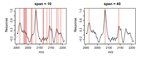
本章中使用的 kohonen 包最初基于类包（Venables 和 Ripley 2002），有几个值得注意的功能尚未讨论（Wehrens 和 Kruisselbrink 2018）。它可以使用通常的欧几里得距离以外的距离函数，这对于某些数据集可能非常有用，通常避免了对先前数据转换的需要。一个例子是前面提到的 WCC 函数：这可用于对一组 X 射线粉末衍射图进行分组，其中峰的位置而不是峰的位置包含主要信息（Wehrens 和 Willighagen 2006；Wehrens 和 Kruisselbrink 2018）。对于数值变量，平方和距离是默认的（比欧几里得距离稍快）；对于因素，谷本距离。在 kohonen 包中，可以提供几个不同的数据层，其中每一层中的行对应于同一对象的不同信息位。可以为每一层定义单独的距离函数，然后使用可由用户定义的权重将其组合成一个整体距离度量。除了本章描述的通常的“在线”训练算法外，还实现了“批量”算法，其中码本向量在所有记录都呈现给地图之前不会更新。批处理算法的一个优点是它省去了 SOM 的参数之一：学习率 然后使用可由用户定义的权重将其组合成一个整体距离度量。除了本章描述的通常的“在线”训练算法外，还实现了“批量”算法，其中码本向量在所有记录都呈现给地图之前不会更新。批处理算法的一个优点是它省去了 SOM 的参数之一：学习率 然后使用可由用户定义的权重将其组合成一个整体距离度量。除了本章描述的通常的“在线”训练算法外，还实现了“批量”算法，其中码本向量在所有记录都呈现给地图之前不会更新。批处理算法的一个优点是它省去了 SOM 的参数之一：学习率一种不再需要。主要缺点是它有时不太稳定，更有可能最终达到局部最优。批处理算法还允许通过将对象与所有码本向量的比较分布在多个内核上进行并行执行（Lawrence et al. 1999），这可能会通过更大的数据集节省大量成本（Wehrens 和 Kruisselbrink 2018）。

统计代写请认准statistics-lab™. statistics-lab™为您的留学生涯保驾护航。

金融工程代写

金融工程是使用数学技术来解决金融问题。金融工程使用计算机科学、统计学、经济学和应用数学领域的工具和知识来解决当前的金融问题，以及设计新的和创新的金融产品。

非参数统计代写

非参数统计指的是一种统计方法，其中不假设数据来自于由少数参数决定的规定模型；这种模型的例子包括正态分布模型和线性回归模型。

广义线性模型代考

广义线性模型（GLM）归属统计学领域，是一种应用灵活的线性回归模型。该模型允许因变量的偏差分布有除了正态分布之外的其它分布。

术语 广义线性模型（GLM）通常是指给定连续和/或分类预测因素的连续响应变量的常规线性回归模型。它包括多元线性回归，以及方差分析和方差分析（仅含固定效应）。

有限元方法代写

有限元方法（FEM）是一种流行的方法，用于数值解决工程和数学建模中出现的微分方程。典型的问题领域包括结构分析、传热、流体流动、质量运输和电磁势等传统领域。

有限元是一种通用的数值方法，用于解决两个或三个空间变量的偏微分方程（即一些边界值问题）。为了解决一个问题，有限元将一个大系统细分为更小、更简单的部分，称为有限元。这是通过在空间维度上的特定空间离散化来实现的，它是通过构建对象的网格来实现的：用于求解的数值域，它有有限数量的点。边界值问题的有限元方法表述最终导致一个代数方程组。该方法在域上对未知函数进行逼近。[1] 然后将模拟这些有限元的简单方程组合成一个更大的方程系统，以模拟整个问题。然后，有限元通过变化微积分使相关的误差函数最小化来逼近一个解决方案。

tatistics-lab作为专业的留学生服务机构，多年来已为美国、英国、加拿大、澳洲等留学热门地的学生提供专业的学术服务，包括但不限于Essay代写，Assignment代写，Dissertation代写，Report代写，小组作业代写，Proposal代写，Paper代写，Presentation代写，计算机作业代写，论文修改和润色，网课代做，exam代考等等。写作范围涵盖高中，本科，研究生等海外留学全阶段，辐射金融，经济学，会计学，审计学，管理学等全球99%专业科目。写作团队既有专业英语母语作者，也有海外名校硕博留学生，每位写作老师都拥有过硬的语言能力，专业的学科背景和学术写作经验。我们承诺100%原创，100%专业，100%准时，100%满意。

随机分析代写

随机微积分是数学的一个分支，对随机过程进行操作。它允许为随机过程的积分定义一个关于随机过程的一致的积分理论。这个领域是由日本数学家伊藤清在第二次世界大战期间创建并开始的。

时间序列分析代写

随机过程，是依赖于参数的一组随机变量的全体，参数通常是时间。 随机变量是随机现象的数量表现，其时间序列是一组按照时间发生先后顺序进行排列的数据点序列。通常一组时间序列的时间间隔为一恒定值（如1秒，5分钟，12小时，7天，1年），因此时间序列可以作为离散时间数据进行分析处理。研究时间序列数据的意义在于现实中，往往需要研究某个事物其随时间发展变化的规律。这就需要通过研究该事物过去发展的历史记录，以得到其自身发展的规律。

回归分析代写

多元回归分析渐进（Multiple Regression Analysis Asymptotics）属于计量经济学领域，主要是一种数学上的统计分析方法，可以分析复杂情况下各影响因素的数学关系，在自然科学、社会和经济学等多个领域内应用广泛。

MATLAB代写

MATLAB 是一种用于技术计算的高性能语言。它将计算、可视化和编程集成在一个易于使用的环境中，其中问题和解决方案以熟悉的数学符号表示。典型用途包括：数学和计算算法开发建模、仿真和原型制作数据分析、探索和可视化科学和工程图形应用程序开发，包括图形用户界面构建MATLAB 是一个交互式系统，其基本数据元素是一个不需要维度的数组。这使您可以解决许多技术计算问题，尤其是那些具有矩阵和向量公式的问题，而只需用 C 或 Fortran 等标量非交互式语言编写程序所需的时间的一小部分。MATLAB 名称代表矩阵实验室。MATLAB 最初的编写目的是提供对由 LINPACK 和 EISPACK 项目开发的矩阵软件的轻松访问，这两个项目共同代表了矩阵计算软件的最新技术。MATLAB 经过多年的发展，得到了许多用户的投入。在大学环境中，它是数学、工程和科学入门和高级课程的标准教学工具。在工业领域，MATLAB 是高效研究、开发和分析的首选工具。MATLAB 具有一系列称为工具箱的特定于应用程序的解决方案。对于大多数 MATLAB 用户来说非常重要，工具箱允许您学习和应用专业技术。工具箱是 MATLAB 函数（M 文件）的综合集合，可扩展 MATLAB 环境以解决特定类别的问题。可用工具箱的领域包括信号处理、控制系统、神经网络、模糊逻辑、小波、仿真等。

R语言代写	问卷设计与分析代写
PYTHON代写	回归分析与线性模型代写
MATLAB代写	方差分析与试验设计代写
STATA代写	机器学习/统计学习代写
SPSS代写	计量经济学代写
EVIEWS代写	时间序列分析代写
EXCEL代写	深度学习代写
SQL代写	各种数据建模与可视化代写

如果你也在 怎样代写化学计量学chemometrics这个学科遇到相关的难题，请随时右上角联系我们的24/7代写客服。

化学计量学是一门化学学科，它使用数学、统计学和其他采用形式逻辑的方法来设计或选择最佳的测量程序和实验，并通过分析化学数据来提供最大的相关化学信息。

将化学计量学方法与经典方法相比较，也许可以最好地理解它的特点。经典方法旨在理解效应–哪些因素是主要的，哪些因素是可以忽略的–而化学计量学方法则放弃了理解效应的必要性，并指出了其他目标，如预测、模式识别、分类等。

statistics-lab™ 为您的留学生涯保驾护航 在代写化学计量学chemometrics方面已经树立了自己的口碑, 保证靠谱, 高质且原创的统计Statistics代写服务。我们的专家在代写化学计量学chemometrics代写方面经验极为丰富，各种代写化学计量学chemometrics相关的作业也就用不着说。

我们提供的化学计量学chemometrics及其相关学科的代写，服务范围广, 其中包括但不限于:

• Statistical Inference 统计推断
• Statistical Computing 统计计算
• Advanced Probability Theory 高等概率论
• Advanced Mathematical Statistics 高等数理统计学
• (Generalized) Linear Models 广义线性模型
• Statistical Machine Learning 统计机器学习
• Longitudinal Data Analysis 纵向数据分析
• Foundations of Data Science 数据科学基础

统计代写|化学计量学作业代写chemometrics代考|Related Methods

PCA is not alone in its aim to find low-dimensional representations of highdimensional data sets. Several other methods try to do the same thing, but rather than finding the projection that maximizes the explained variance, they choose other criteria. In Principal Coordinate Analysis (PCoA) and the related Multidimensional Scaling (MDS) methods, the aim is to find a low-dimensional projection that reproduces the experimentally found distances between the data points. When these distances are Euclidean, the results are the same or very similar to PCA results; however, other distances can be used as well. Independent Component Analysis maximizes deviations from normality rather than variance, and Factor Analysis concentrates on reproducing covariances. We will briefly review these methods in the next paragraphs.

统计代写|化学计量学作业代写chemometrics代考|Multidimensional Scaling

In some cases, applying PCA to the raw data matrix is not appropriate, for example in situations where regular Euclidean distances do not apply-similarities between chemical structures, e.g., can be expressed easily in several different ways, but it is not at all clear how to represent molecules into fixed-length structure descriptors (Baumann 1999), something that is required by distance measures such as the Euclidean distance. Even when comparing spectra or chromatograms, the Euclidean distance can be inappropriate, for instance in the presence of peak shifts (Bloemberg et al. 2010 ; de Gelder et al. 2001). In other cases, raw data are simply not available and the only information one has consists of similarities. Based on the sample similarities, the goal of methods like Multidimensional Scaling (MDS, (Borg and Groenen 2005; Cox and Cox 2001)) is to reconstruct a low-dimensional map of samples that leads to the same similarity matrix as the original data (or a very close approximation).

Since visualization usually is one of the main aims, the number of dimensions usually is set to two, but in principle one could find an optimal configuration with other dimensionalities as well.

The problem is something like making a topographical map, given only the distances between the cities in the country. In this case, an exact solution is possible in two dimensions since the original distance matrix was calculated from twodimensional coordinates. Note that although distances can be reproduced exactly, the map still has rotational and translational freedom-in practice this does not pose any problems, however. An amusing example is given by maps not based on kilometers but rather on travel time-the main cities will be moved to the center of the plot since they usually are connected by high-speed trains, whereas smaller villages will appear to be further away. In such a case, and in virtually all practical applications, a two-dimensional plot will not be able to reproduce all similarities exactly.

In MDS, there are several ways to indicate the agreement between the two distance matrices, and these lead to different methods. The simplest approach is to perform $\mathrm{PCA}$ on the double-centered distance matrix, ${ }^{4}$ an approach that is known as Principal Coordinate Analysis, or Classical MDS (Gower 1966). The criterion to be minimized is called the stress, and is given by
$$
S=\sum_{j<i}\left(\left|x_{i}-x_{j}\right|-e_{i j}\right)^{2}=\sum_{j<i}\left(d_{i j}-e_{i j}\right)^{2}
$$
where $e_{i j}$ corresponds with the true, given, distances, and $d_{i j}$ are the distances between objects $x_{i}$ and $x_{j}$ in the low-dimensional space.

统计代写|化学计量学作业代写chemometrics代考|Independent Component Analysis and Projection Pursuit

Variation in many cases equals information, one of the reasons behind the widespread application of PCA. Or, to put it the other way around, a variable that has a constant value does not provide much information. However, there are many examples where the relevant information is hidden in small differences, and is easily overwhelmed by other sources of variation that are of no interest. The technique of Projection Pursuit (Friedman 1987; Friedman and Tukey 1974; Huber 1985) is a generalization of PCA where a number of different criteria can be optimized. One can for instance choose a viewpoint that maximizes some grouping in the data. In general, however, there is no analytical solution for any of these criteria, except for the variance criterion used in PCA. A special case of Projection Pursuit is Independent Component Analysis (ICA, Hyvärinen et al. 2001), where the view is taken to maximize deviation from multivariate normality, given by the negentropy $J$. This is the difference of the entropy of a normally distributed random variable $H\left(x_{\mathrm{G}}\right)$ and the entropy of the variable under consideration $H(x)$
$$
J(x)=H\left(x_{\mathrm{G}}\right)-H(x)
$$
where the entropy itself is given by
$$
H(x)=-\int f(x) \log f(x) d x
$$
Since the entropy of a normally distributed variable is maximal, the negentropy is always positive (Cover and Thomas 1991). Unfortunately, this quantity is hard to calculate, and in practice approximations, such as kurtosis and the fourth moment are used.

化学计量学代写

统计代写|化学计量学作业代写chemometrics代考|Related Methods

PCA 并不是唯一一个致力于寻找高维数据集的低维表示的人。其他几种方法尝试做同样的事情，但不是找到最大化解释方差的投影，而是选择其他标准。在主坐标分析 (PCoA) 和相关的多维缩放 (MDS) 方法中，目标是找到一个低维投影，该投影再现实验发现的数据点之间的距离。当这些距离为欧式时，结果与 PCA 结果相同或非常相似；然而，也可以使用其他距离。独立成分分析最大限度地偏离正态性而不是方差，因子分析专注于再现协方差。我们将在接下来的段落中简要回顾这些方法。

统计代写|化学计量学作业代写chemometrics代考|Multidimensional Scaling

在某些情况下，将 PCA 应用于原始数据矩阵是不合适的，例如在不适用常规欧几里德距离的情况下 – 化学结构之间的相似性，例如，可以很容易地以几种不同的方式表达，但根本不清楚如何将分子表示为固定长度的结构描述符（Baumann 1999），这是距离度量（如欧几里得距离）所要求的。即使在比较光谱或色谱图时，欧几里得距离也可能不合适，例如在存在峰移的情况下（Bloemberg 等人 2010 ；de Gelder 等人 2001）。在其他情况下，原始数据根本不可用，唯一的信息是相似性。基于样本相似性，多维缩放（MDS，（Borg and Groenen 2005；

由于可视化通常是主要目标之一，因此维度的数量通常设置为两个，但原则上也可以找到具有其他维度的最佳配置。

问题类似于制作地形图，只考虑该国城市之间的距离。在这种情况下，由于原始距离矩阵是根据二维坐标计算的，因此可以在二维中得到精确解。请注意，尽管距离可以精确再现，但地图仍然具有旋转和平移自由度——然而，这在实践中不会造成任何问题。一个有趣的例子是地图不是基于公里，而是基于旅行时间——主要城市将被移动到情节的中心，因为它们通常由高速火车连接，而较小的村庄似乎更远。在这种情况下，几乎在所有实际应用中，二维图都无法准确再现所有相似性。

在 MDS 中，有几种方法可以表示两个距离矩阵之间的一致性，这些方法导致了不同的方法。最简单的方法是执行磷C一种在双中心距离矩阵上，4一种称为主坐标分析或经典 MDS 的方法 (Gower 1966)。要最小化的标准称为应力，由下式给出
小号=∑j<一世(|X一世−Xj|−和一世j)2=∑j<一世(d一世j−和一世j)2
在哪里和一世j对应于真实的、给定的距离，并且d一世j是物体之间的距离X一世和Xj在低维空间。

统计代写|化学计量学作业代写chemometrics代考|Independent Component Analysis and Projection Pursuit

在许多情况下，变化等于信息，这是 PCA 广泛应用的原因之一。或者，换句话说，具有恒定值的变量不会提供太多信息。然而，有很多例子表明相关信息隐藏在微小的差异中，并且很容易被其他不感兴趣的变异来源所淹没。Projection Pursuit 技术（Friedman 1987；Friedman and Tukey 1974；Huber 1985）是 PCA 的推广，可以优化许多不同的标准。例如，可以选择一种观点，使数据中的某些分组最大化。然而，一般来说，这些标准中的任何一个都没有解析解，除了 PCA 中使用的方差标准。Projection Pursuit 的一个特例是独立分量分析 (ICA, Hyvärinen 等人。2001），其中观点被认为是最大化与多元正态性的偏差，由负熵给出Ĵ. 这是正态分布随机变量的熵之差H(XG)和所考虑变量的熵H(X)
Ĵ(X)=H(XG)−H(X)
其中熵本身由下式给出
H(X)=−∫F(X)日志⁡F(X)dX
由于正态分布变量的熵最大，因此负熵始终为正（Cover 和 Thomas 1991）。不幸的是，这个量很难计算，并且在实践中使用了近似值，例如峰度和四阶矩。

统计代写请认准statistics-lab™. statistics-lab™为您的留学生涯保驾护航。

金融工程代写

金融工程是使用数学技术来解决金融问题。金融工程使用计算机科学、统计学、经济学和应用数学领域的工具和知识来解决当前的金融问题，以及设计新的和创新的金融产品。

非参数统计代写

非参数统计指的是一种统计方法，其中不假设数据来自于由少数参数决定的规定模型；这种模型的例子包括正态分布模型和线性回归模型。

广义线性模型代考

广义线性模型（GLM）归属统计学领域，是一种应用灵活的线性回归模型。该模型允许因变量的偏差分布有除了正态分布之外的其它分布。

术语 广义线性模型（GLM）通常是指给定连续和/或分类预测因素的连续响应变量的常规线性回归模型。它包括多元线性回归，以及方差分析和方差分析（仅含固定效应）。

有限元方法代写

有限元方法（FEM）是一种流行的方法，用于数值解决工程和数学建模中出现的微分方程。典型的问题领域包括结构分析、传热、流体流动、质量运输和电磁势等传统领域。

有限元是一种通用的数值方法，用于解决两个或三个空间变量的偏微分方程（即一些边界值问题）。为了解决一个问题，有限元将一个大系统细分为更小、更简单的部分，称为有限元。这是通过在空间维度上的特定空间离散化来实现的，它是通过构建对象的网格来实现的：用于求解的数值域，它有有限数量的点。边界值问题的有限元方法表述最终导致一个代数方程组。该方法在域上对未知函数进行逼近。[1] 然后将模拟这些有限元的简单方程组合成一个更大的方程系统，以模拟整个问题。然后，有限元通过变化微积分使相关的误差函数最小化来逼近一个解决方案。

tatistics-lab作为专业的留学生服务机构，多年来已为美国、英国、加拿大、澳洲等留学热门地的学生提供专业的学术服务，包括但不限于Essay代写，Assignment代写，Dissertation代写，Report代写，小组作业代写，Proposal代写，Paper代写，Presentation代写，计算机作业代写，论文修改和润色，网课代做，exam代考等等。写作范围涵盖高中，本科，研究生等海外留学全阶段，辐射金融，经济学，会计学，审计学，管理学等全球99%专业科目。写作团队既有专业英语母语作者，也有海外名校硕博留学生，每位写作老师都拥有过硬的语言能力，专业的学科背景和学术写作经验。我们承诺100%原创，100%专业，100%准时，100%满意。

随机分析代写

随机微积分是数学的一个分支，对随机过程进行操作。它允许为随机过程的积分定义一个关于随机过程的一致的积分理论。这个领域是由日本数学家伊藤清在第二次世界大战期间创建并开始的。

时间序列分析代写

随机过程，是依赖于参数的一组随机变量的全体，参数通常是时间。 随机变量是随机现象的数量表现，其时间序列是一组按照时间发生先后顺序进行排列的数据点序列。通常一组时间序列的时间间隔为一恒定值（如1秒，5分钟，12小时，7天，1年），因此时间序列可以作为离散时间数据进行分析处理。研究时间序列数据的意义在于现实中，往往需要研究某个事物其随时间发展变化的规律。这就需要通过研究该事物过去发展的历史记录，以得到其自身发展的规律。

回归分析代写

多元回归分析渐进（Multiple Regression Analysis Asymptotics）属于计量经济学领域，主要是一种数学上的统计分析方法，可以分析复杂情况下各影响因素的数学关系，在自然科学、社会和经济学等多个领域内应用广泛。

MATLAB代写

MATLAB 是一种用于技术计算的高性能语言。它将计算、可视化和编程集成在一个易于使用的环境中，其中问题和解决方案以熟悉的数学符号表示。典型用途包括：数学和计算算法开发建模、仿真和原型制作数据分析、探索和可视化科学和工程图形应用程序开发，包括图形用户界面构建MATLAB 是一个交互式系统，其基本数据元素是一个不需要维度的数组。这使您可以解决许多技术计算问题，尤其是那些具有矩阵和向量公式的问题，而只需用 C 或 Fortran 等标量非交互式语言编写程序所需的时间的一小部分。MATLAB 名称代表矩阵实验室。MATLAB 最初的编写目的是提供对由 LINPACK 和 EISPACK 项目开发的矩阵软件的轻松访问，这两个项目共同代表了矩阵计算软件的最新技术。MATLAB 经过多年的发展，得到了许多用户的投入。在大学环境中，它是数学、工程和科学入门和高级课程的标准教学工具。在工业领域，MATLAB 是高效研究、开发和分析的首选工具。MATLAB 具有一系列称为工具箱的特定于应用程序的解决方案。对于大多数 MATLAB 用户来说非常重要，工具箱允许您学习和应用专业技术。工具箱是 MATLAB 函数（M 文件）的综合集合，可扩展 MATLAB 环境以解决特定类别的问题。可用工具箱的领域包括信号处理、控制系统、神经网络、模糊逻辑、小波、仿真等。

R语言代写	问卷设计与分析代写
PYTHON代写	回归分析与线性模型代写
MATLAB代写	方差分析与试验设计代写
STATA代写	机器学习/统计学习代写
SPSS代写	计量经济学代写
EVIEWS代写	时间序列分析代写
EXCEL代写	深度学习代写
SQL代写	各种数据建模与可视化代写

如果你也在 怎样代写化学计量学chemometrics这个学科遇到相关的难题，请随时右上角联系我们的24/7代写客服。

化学计量学是一门化学学科，它使用数学、统计学和其他采用形式逻辑的方法来设计或选择最佳的测量程序和实验，并通过分析化学数据来提供最大的相关化学信息。

将化学计量学方法与经典方法相比较，也许可以最好地理解它的特点。经典方法旨在理解效应–哪些因素是主要的，哪些因素是可以忽略的–而化学计量学方法则放弃了理解效应的必要性，并指出了其他目标，如预测、模式识别、分类等。

statistics-lab™ 为您的留学生涯保驾护航 在代写化学计量学chemometrics方面已经树立了自己的口碑, 保证靠谱, 高质且原创的统计Statistics代写服务。我们的专家在代写化学计量学chemometrics代写方面经验极为丰富，各种代写化学计量学chemometrics相关的作业也就用不着说。

我们提供的化学计量学chemometrics及其相关学科的代写，服务范围广, 其中包括但不限于:

• Statistical Inference 统计推断
• Statistical Computing 统计计算
• Advanced Probability Theory 高等概率论
• Advanced Mathematical Statistics 高等数理统计学
• (Generalized) Linear Models 广义线性模型
• Statistical Machine Learning 统计机器学习
• Longitudinal Data Analysis 纵向数据分析
• Foundations of Data Science 数据科学基础

统计代写|化学计量学作业代写chemometrics代考|The Machinery

Currently, PCA is implemented even in low-level numerical software such as spreadsheets. Nevertheless, it is good to know the basics behind the computations. In almost all cases, the algorithm used to calculate the PCs is Singular Value Decomposition (SVD). ${ }^{2}$ It decomposes an $n \times p$ mean-centered data matrix $\boldsymbol{X}$ into three parts:
$$
\boldsymbol{X}=\boldsymbol{U} \boldsymbol{D} \boldsymbol{V}^{T}
$$
where $\boldsymbol{U}$ is a $n \times a$ orthonormal matrix containing the left singular vectors, $\boldsymbol{D}$ is a diagonal matrix $(a \times a$ ) containing the singular values, and $V$ is a $p \times a$ orthonormal matrix containing the right singular vectors. The latter are what in PCA terminology is called the loadings-the product of the first two matrices forms the scores:
$$
\boldsymbol{X}=(\boldsymbol{U} \boldsymbol{D}) \boldsymbol{V}^{T}=\boldsymbol{T} \boldsymbol{P}^{T}
$$
The interpretation of matrices $T, P, U, D$ and $V$ is straightforward. The loadings, columns in matrix $\boldsymbol{P}$ (or equivalently, the right singular vectors, columns in matrix $V$ ) give the weights of the original variables in the PCs. Variables that have very low values in a specific column of $\boldsymbol{V}$ contribute only very little to that particular latent variable. The scores, columns in $T$, constitute the coordinates in the space of the latent variables. Put differently: these are the coordinates of the samples as we see them from our new PCA viewpoint. The columns in $\boldsymbol{U}$ give the same coordinates in a normalized form – they have unit variances, whereas the columns in $T$ have variances corresponding to the variances of each particular PC. These variances $\lambda_{i}$ are proportional to the squares of the diagonal elements in matrix $\boldsymbol{D}$ :
$$
\lambda_{i}=d_{i}^{2} /(n-1)
$$
The fraction of variance explained by PC $i$ can therefore be expressed as
$$
F V(i)=\lambda_{i} / \sum_{j=1}^{a} \lambda_{j}
$$
One main problem in the application of PCA is the decision on how many PCs to retain; we will come back to this in Section 4.3.

统计代写|化学计量学作业代写chemometrics代考|Doing It Yourself

Calculating scores and loadings is easy: consider the wine data first. We perform PCA on the autoscaled data to remove the effects of the different scales of the variables using the svd function provided by $R$ :

• wines.svd <- svd (wines. sc)
• wines. scores <- wines . svdș q t

wines. loadings <- wines.svd\$v The first two PCs represent the plane that contains most of the variance; how much exactly is given by the squares of the values on the diagonal of $\boldsymbol{D}$. The importance of individual PCs is usually given by the percentage of the overall variance that is explained: $>$ wines. vars <-wines . svd\$ $\mathrm{d}^{n} 2 /$ (nrow (wines) – 1)
wines.totalvar <- sum (wines.vars)
wines.relvars <- wines. vars / wines.totalvar
variances <- 100 * round (wines . relvars, digits = 3)
variances [1:5]
[1] $36.0 \quad 19.2 \quad 11.2 \quad 7.1 \quad 6.6$
The first PC covers more than one third of the total variance; for the fifth PC this amount is down to one fifteenth.

统计代写|化学计量学作业代写chemometrics代考|Scree Plots

The amount of variance per PC is usually depicted in a scree plot: either the variances themselves or the logarithms of the variances are shown as bars. Often, one also considers the fraction of the total variance explained by every single PC. The last few PCs usually contain no information and, especially on a log scale, tend to make the scree plot less interpretable, so they are usually not taken into account in the plot.
$>$ barplot (wines, $\operatorname{vars}[1: 10]$, main = “Variances”,
names.arg = paste (“PC”, 1:10))
barplot(log (wines. vars $[1: 10])$, main = “log (Variances) “,
names.arg = paste (“PC”, 1:10))

barplot(wines. relvars $[1: 10]$, main = “Relative variances”,
names.arg = paste $(” \mathrm{PC} “, 1: 10))$
b barplot (cumsum $(100$ * wines. relvars $[1: 10])$ ).
main = “Cumulative variances (8)”,
names $\cdot a r g=$ paste( “PC”, 1:10), ylim $=c(0,100))$
This leads to the plots in Fig. 4.2. Clearly, PCs 1 and 2 explain much more variance than the others: together they cover $55 \%$ of the variance. The scree plots show no clear cut-off, which in real life is the rule rather than the exception. Depending on the goal of the investigation, for these data one could consider three or five PCs. Choosing four PCs would not make much sense in this case, since the fifth PC would explain almost the same amount of variance: if the fourth is included, the fifth should be, too.

化学计量学代写

统计代写|化学计量学作业代写chemometrics代考|The Machinery

目前，即使在电子表格等低级数值软件中也实现了 PCA。不过，最好了解计算背后的基础知识。在几乎所有情况下，用于计算 PC 的算法都是奇异值分解 (SVD)。2它分解一个n×p均值中心数据矩阵X分为三个部分：
X=在D在吨
在哪里在是一个n×一种包含左奇异向量的正交矩阵，D是对角矩阵(一种×一种) 包含奇异值，并且在是一个p×一种包含右奇异向量的正交矩阵。后者在 PCA 术语中称为载荷——前两个矩阵的乘积形成分数：
X=(在D)在吨=吨磷吨
矩阵的解释吨,磷,在,D和在很简单。矩阵中的载荷、列磷（或等效地，右奇异向量，矩阵中的列在) 给出 PC 中原始变量的权重。在特定列中具有非常低值的变量在对该特定潜在变量的贡献很小。分数，列吨，构成潜变量空间中的坐标。换句话说：这些是我们从新的 PCA 角度看到的样本的坐标。中的列在以标准化形式给出相同的坐标——它们有单位方差，而吨具有对应于每个特定 PC 的方差的方差。这些差异λ一世与矩阵中对角线元素的平方成正比D :
λ一世=d一世2/(n−1)
PC 解释的方差分数一世因此可以表示为
F在(一世)=λ一世/∑j=1一种λj
PCA 应用的一个主要问题是决定保留多少 PC；我们将在第 4.3 节中回到这一点。

统计代写|化学计量学作业代写chemometrics代考|Doing It Yourself

计算分数和负荷很容易：首先考虑葡萄酒数据。我们对自动缩放的数据执行 PCA，以使用由R:

• wines.svd <- svd (wines.sc)
• 葡萄酒。分数 <- 葡萄酒。svd qt

葡萄酒。loadings <- wines.svd $ v 前两个 PC 代表包含大部分方差的平面；多少是由对角线上的值的平方给出的D. 单个 PC 的重要性通常由解释的总体方差的百分比给出：>葡萄酒。变量 <-葡萄酒。美元_ dn2/(nrow (wines) – 1)
wines.totalvar <- sum (wines.vars)
wines.relvars <- wines。vars / wines.totalvar
方差 <- 100 * round (wines . relvars, digits = 3)
方差 [1:5]
[1]36.019.211.27.16.6
第一个PC覆盖了总方差的三分之一以上；对于第五台个人电脑，这一数额降至十五分之一。

统计代写|化学计量学作业代写chemometrics代考|Scree Plots

每台 PC 的方差量通常在碎石图中描述：方差本身或方差的对数显示为条形。通常，人们还会考虑每台 PC 解释的总方差的比例。最后几台 PC 通常不包含任何信息，尤其是在对数尺度上，往往会使碎石图难以解释，因此通常不会在图中考虑它们。
>条形图（葡萄酒，谁的⁡[1:10], main = “Variances”,
names.arg = paste (“PC”, 1:10))
barplot(log (wines.vars[1:10]), main = “log (Variances)”,
names.arg = paste (“PC”, 1:10))

条形图（葡萄酒。relvars[1:10], main = “相对方差”,
names.arg = paste(”磷C“,1:10))
b条形图（cumsum(100* 葡萄酒。相关人员[1:10])）。
main = “累积方差 (8)”，
名称⋅一种rG=粘贴（“PC”，1:10），同上=C(0,100))
这导致图 4.2 中的图。显然，PC 1 和 2 比其他的解释了更多的差异：它们一起涵盖55%的方差。碎石图没有明确的界限，这在现实生活中是规则而不是例外。根据调查的目标，对于这些数据，可以考虑三到五台 PC。在这种情况下，选择四台 PC 没有多大意义，因为第五台 PC 可以解释几乎相同数量的方差：如果包括第四台，那么第五台也应该包括在内。

统计代写请认准statistics-lab™. statistics-lab™为您的留学生涯保驾护航。

金融工程代写

金融工程是使用数学技术来解决金融问题。金融工程使用计算机科学、统计学、经济学和应用数学领域的工具和知识来解决当前的金融问题，以及设计新的和创新的金融产品。

非参数统计代写

非参数统计指的是一种统计方法，其中不假设数据来自于由少数参数决定的规定模型；这种模型的例子包括正态分布模型和线性回归模型。

广义线性模型代考

广义线性模型（GLM）归属统计学领域，是一种应用灵活的线性回归模型。该模型允许因变量的偏差分布有除了正态分布之外的其它分布。

术语 广义线性模型（GLM）通常是指给定连续和/或分类预测因素的连续响应变量的常规线性回归模型。它包括多元线性回归，以及方差分析和方差分析（仅含固定效应）。

有限元方法代写

有限元方法（FEM）是一种流行的方法，用于数值解决工程和数学建模中出现的微分方程。典型的问题领域包括结构分析、传热、流体流动、质量运输和电磁势等传统领域。

有限元是一种通用的数值方法，用于解决两个或三个空间变量的偏微分方程（即一些边界值问题）。为了解决一个问题，有限元将一个大系统细分为更小、更简单的部分，称为有限元。这是通过在空间维度上的特定空间离散化来实现的，它是通过构建对象的网格来实现的：用于求解的数值域，它有有限数量的点。边界值问题的有限元方法表述最终导致一个代数方程组。该方法在域上对未知函数进行逼近。[1] 然后将模拟这些有限元的简单方程组合成一个更大的方程系统，以模拟整个问题。然后，有限元通过变化微积分使相关的误差函数最小化来逼近一个解决方案。

tatistics-lab作为专业的留学生服务机构，多年来已为美国、英国、加拿大、澳洲等留学热门地的学生提供专业的学术服务，包括但不限于Essay代写，Assignment代写，Dissertation代写，Report代写，小组作业代写，Proposal代写，Paper代写，Presentation代写，计算机作业代写，论文修改和润色，网课代做，exam代考等等。写作范围涵盖高中，本科，研究生等海外留学全阶段，辐射金融，经济学，会计学，审计学，管理学等全球99%专业科目。写作团队既有专业英语母语作者，也有海外名校硕博留学生，每位写作老师都拥有过硬的语言能力，专业的学科背景和学术写作经验。我们承诺100%原创，100%专业，100%准时，100%满意。

随机分析代写

随机微积分是数学的一个分支，对随机过程进行操作。它允许为随机过程的积分定义一个关于随机过程的一致的积分理论。这个领域是由日本数学家伊藤清在第二次世界大战期间创建并开始的。

时间序列分析代写

随机过程，是依赖于参数的一组随机变量的全体，参数通常是时间。 随机变量是随机现象的数量表现，其时间序列是一组按照时间发生先后顺序进行排列的数据点序列。通常一组时间序列的时间间隔为一恒定值（如1秒，5分钟，12小时，7天，1年），因此时间序列可以作为离散时间数据进行分析处理。研究时间序列数据的意义在于现实中，往往需要研究某个事物其随时间发展变化的规律。这就需要通过研究该事物过去发展的历史记录，以得到其自身发展的规律。

回归分析代写

多元回归分析渐进（Multiple Regression Analysis Asymptotics）属于计量经济学领域，主要是一种数学上的统计分析方法，可以分析复杂情况下各影响因素的数学关系，在自然科学、社会和经济学等多个领域内应用广泛。

MATLAB代写

MATLAB 是一种用于技术计算的高性能语言。它将计算、可视化和编程集成在一个易于使用的环境中，其中问题和解决方案以熟悉的数学符号表示。典型用途包括：数学和计算算法开发建模、仿真和原型制作数据分析、探索和可视化科学和工程图形应用程序开发，包括图形用户界面构建MATLAB 是一个交互式系统，其基本数据元素是一个不需要维度的数组。这使您可以解决许多技术计算问题，尤其是那些具有矩阵和向量公式的问题，而只需用 C 或 Fortran 等标量非交互式语言编写程序所需的时间的一小部分。MATLAB 名称代表矩阵实验室。MATLAB 最初的编写目的是提供对由 LINPACK 和 EISPACK 项目开发的矩阵软件的轻松访问，这两个项目共同代表了矩阵计算软件的最新技术。MATLAB 经过多年的发展，得到了许多用户的投入。在大学环境中，它是数学、工程和科学入门和高级课程的标准教学工具。在工业领域，MATLAB 是高效研究、开发和分析的首选工具。MATLAB 具有一系列称为工具箱的特定于应用程序的解决方案。对于大多数 MATLAB 用户来说非常重要，工具箱允许您学习和应用专业技术。工具箱是 MATLAB 函数（M 文件）的综合集合，可扩展 MATLAB 环境以解决特定类别的问题。可用工具箱的领域包括信号处理、控制系统、神经网络、模糊逻辑、小波、仿真等。

R语言代写	问卷设计与分析代写
PYTHON代写	回归分析与线性模型代写
MATLAB代写	方差分析与试验设计代写
STATA代写	机器学习/统计学习代写
SPSS代写	计量经济学代写
EVIEWS代写	时间序列分析代写
EXCEL代写	深度学习代写
SQL代写	各种数据建模与可视化代写

如果你也在 怎样代写化学计量学chemometrics这个学科遇到相关的难题，请随时右上角联系我们的24/7代写客服。

化学计量学是一门化学学科，它使用数学、统计学和其他采用形式逻辑的方法来设计或选择最佳的测量程序和实验，并通过分析化学数据来提供最大的相关化学信息。

将化学计量学方法与经典方法相比较，也许可以最好地理解它的特点。经典方法旨在理解效应–哪些因素是主要的，哪些因素是可以忽略的–而化学计量学方法则放弃了理解效应的必要性，并指出了其他目标，如预测、模式识别、分类等。

statistics-lab™ 为您的留学生涯保驾护航 在代写化学计量学chemometrics方面已经树立了自己的口碑, 保证靠谱, 高质且原创的统计Statistics代写服务。我们的专家在代写化学计量学chemometrics代写方面经验极为丰富，各种代写化学计量学chemometrics相关的作业也就用不着说。

我们提供的化学计量学chemometrics及其相关学科的代写，服务范围广, 其中包括但不限于:

• Statistical Inference 统计推断
• Statistical Computing 统计计算
• Advanced Probability Theory 高等概率论
• Advanced Mathematical Statistics 高等数理统计学
• (Generalized) Linear Models 广义线性模型
• Statistical Machine Learning 统计机器学习
• Longitudinal Data Analysis 纵向数据分析
• Foundations of Data Science 数据科学基础

统计代写|化学计量学作业代写chemometrics代考|Scaling

The scaling method that is employed can totally change the result of an analysis. One should therefore carefully consider what scaling method (if any) is appropriate. Scaling can serve several purposes. Many analytical methods provide data that are not on an absolute scale; the raw data in such a case cannot be used directly when comparing different samples. If some kind of internal standard is present, it can be used to calibrate the intensities. In NMR, for instance, the TMS (tetramethylsilane, added to indicate the position of the origin on the $x$-axis) peak can be used for this if its concentration is known. Peak heights can then be compared directly. However, even in that situation it may be necessary to further scale intensities, since samples may contain different concentrations. A good example is the analysis of a set of urine samples by NMR. These samples will show appreciable global differences in concentrations, perhaps due to the amount of liquid the individuals have been consuming. This usually is not of interest-rather, one seeks one or perhaps a couple of metabolites with concentrations that deviate from the general pattern. As an example, consider the first ten spectra of the prostate data:

The intensity differences within these first ten spectra are already a factor five for both statistics. If these differences are not related to the phenomenon we are interested in but are caused, e.g., by the nature of the measurements, then it is important to remove them. As stated earlier, also in cases where alignment is necessary, this type of differences between samples can hamper the analysis.

Several options exist to make peak intensities comparable over a series of spectra. The most often-used are range scaling, length scaling and variance scaling. In range scaling, one makes sure that the data have the same minimal and maximal values. Often, only the maximal value is considered important since for many forms of spectroscopy zero is the natural lower bound. Length scaling sets the length of each spectrum to one; variance scaling sets the variance to one. The implementation in $R$ is easy. Here, these three methods are shown for the first ten spectra of the prostate data. Range scaling can be performed by

The sweep function is very similar to apply-it performs an action for every row or column of a data matrix. The MARGIN argument states which dimension is affected. In this case the MARGIN $=1$ indicates the rows; column-wise sweeping would be achieved with MARGIN $=2$. The third argument is the statistic that is to be swept out, here the vector of the per-row maximal values. The final argument states how the sweeping is to be done. The default is to use subtraction; here we use division. Clearly, the differences between the spectra have decreased.

统计代写|化学计量学作业代写chemometrics代考|Missing Data

Missing data are measurements that for some reason have not led to a valid result. In spectroscopic measurements, missing data are not usually encountered, but in many other areas of science they occur frequently. The main question to be answered is: are the data missing at random? If yes, then we can probably get around the problem, provided there are not too many missing data. If not, then it means that there is some rationale behind the missingness of data points. If we would know what it was, we could use that to decide how to handle the missing values. Usually, we don’t, and that means trouble: if the missingness is related to the process we are studying our results will be biased and we can never be sure we are drawing correct conclusions.
Missing values in R are usually indicated by NA. Since many types of analysis do not accept data containing NAs, it is necessary to think of how to handle the missing values. If there are only a few, and they occur mostly in one or a few samples or one or a few variables, we might want to leave out these samples (or variables). Especially when the data set is rather large this seems a small price to pay for the luxury of having complete freedom in choosing any analysis method that is suited to our aim. Alternatively, one can try to find suitable replacements for the missing values, e.g. by estimating them from the other data points, a process that is known as imputation. Intermediate approaches are also possible, in which variables or samples with too many missing values are removed, and others, with a lower fraction of missing data, are retained. Sometimes imputation is not needed for statistical analysis: fitting linear models with $1 \mathrm{~m}$ for instance is possible also in the presence of missing values – these data points will simply be ignored in the fit process. Other functions such as var and cor have arguments that define several ways of dealing with missing values. In var, the argument is na. rm, allowing the user to either throw out missing values or accept missing values in the result, whereas cor has a more elaborate mechanism of defining strategies to deal with missing values. For instance, one can choose to consider only complete cases, or use only pairwise complete observations. Consult the manual pages for more information and examples. One example of dealing with missing values is shown in Sect. 11.1.

统计代写|化学计量学作业代写chemometrics代考|Principal Component Analysis

Principal Component Analysis or PCA (Jackson 1991; Jolliffe 1986) is a technique which, quite literally, takes a different viewpoint of multivariate data. It has many uses, perhaps the most important of which is the possibility to provide simple twodimensional plots of high-dimensional data. This way, one can easily assess the presence of grouping or outliers, and more generally obtain an idea of how samples and variables relate to each other. PCA defines new variables, consisting of linear combinations of the original ones, in such a way that the first axis is in the direction containing most variation. Every subsequent new variable is orthogonal to previous variables, but again in the direction containing most of the remaining variation. The new variables are examples of what is called latent variables (LVs) – in the context of PCA the term principal components (PCs) is used.

The central idea is that more often than not many of the variables in highdimensional data are superfluous. If we look at high-resolution spectra, for example, it is immediately obvious that neighboring wavelengths are highly correlated and contain similar information. Of course, one can try to pick only those wavelengths that appear to be informative, or at least differ from the other wavelengths in the selected set. This could, e.g., be based on clustering the variables, and selecting for each cluster one “representative”. However, this approach is quite elaborate and will lead to different results when using different clustering methods and cutting criteria. Another approach is to use variable selection, given some criterion-one example is to select a limited set of variables leading to a matrix with maximal rank. Variable selection is notoriously difficult, especially in high-dimensional cases. In practice, many more or less equivalent solutions exist, which makes the interpretation quite difficult. We will come back to variable selection methods in Chap. $10 .$

PCA is an alternative. It provides a direct mapping of high-dimensional data into a lower-dimensional space containing most of the information in the original data. The tacit assumption here is that variation equals information. This is not always true, since variation may also be totally meaningless, e.g., in the case of noise. ${ }^{1}$ The coordinates of the samples in the new space are called scores, often indicated with the symbol $T$. The new dimensions are linear combinations of the original variables, and are called loadings (symbol $\boldsymbol{P}$ ). The term Principal Component ( $\mathrm{PC}$ ) can refer to both scores and loadings; which is meant is usually clear from the context. Thus, one can speak of sample coordinates in the space spanned by PC 1 and 2 , but also of variables contributing greatly to $\mathrm{PC} 1$.

化学计量学代写

统计代写|化学计量学作业代写chemometrics代考|Scaling

采用的缩放方法可以完全改变分析的结果。因此，应该仔细考虑哪种缩放方法（如果有的话）是合适的。缩放可以用于多种目的。许多分析方法提供的数据不是绝对的；这种情况下的原始数据在比较不同样本时不能直接使用。如果存在某种内标，它可用于校准强度。例如，在 NMR 中，添加 TMS（四甲基硅烷，用于指示原点的位置）X轴）峰可以用于此，如果它的浓度是已知的。然后可以直接比较峰高。然而，即使在这种情况下，也可能需要进一步缩放强度，因为样品可能包含不同的浓度。一个很好的例子是通过 NMR 分析一组尿液样本。这些样本将显示出明显的全球浓度差异，这可能是由于个体消耗的液体量。这通常是不感兴趣的，而是寻找一种或几种浓度偏离一般模式的代谢物。例如，考虑前列腺数据的前十个光谱：

这前十个光谱中的强度差异已经是两个统计数据的五倍。如果这些差异与我们感兴趣的现象无关，而是由测量的性质引起的，那么消除它们很重要。如前所述，同样在需要对齐的情况下，样本之间的这种差异也会妨碍分析。

有几种选择可以使峰强度在一系列光谱上具有可比性。最常用的是范围缩放、长度缩放和方差缩放。在范围缩放中，确保数据具有相同的最小值和最大值。通常，只有最大值被认为是重要的，因为对于许多形式的光谱学来说，零是自然的下限。长度缩放将每个光谱的长度设置为 1；方差缩放将方差设置为 1。中的实施R简单。在这里，这三种方法显示为前列腺数据的前十个光谱。范围缩放可以通过

扫描功能与应用非常相似——它对数据矩阵的每一行或每一列执行一个动作。MARGIN 参数说明了受影响的维度。在这种情况下，保证金=1表示行；使用 MARGIN 可以实现逐列扫描=2. 第三个参数是要清除的统计量，这里是每行最大值的向量。最后一个论点说明了如何进行清扫。默认使用减法；这里我们使用除法。显然，光谱之间的差异已经减小。

统计代写|化学计量学作业代写chemometrics代考|Missing Data

缺失数据是由于某种原因没有得出有效结果的测量值。在光谱测量中，通常不会遇到丢失数据，但在许多其他科学领域中，它们经常发生。要回答的主要问题是：数据是否随机丢失？如果是，那么我们可能可以解决这个问题，前提是没有太多丢失的数据。如果不是，那么这意味着数据点缺失背后有一些基本原理。如果我们知道它是什么，我们可以用它来决定如何处理缺失值。通常，我们不这样做，这意味着麻烦：如果缺失与我们正在研究的过程有关，我们的结果将是有偏差的，我们永远无法确定我们得出了正确的结论。
R 中的缺失值通常用 NA 表示。由于许多类型的分析不接受包含 NA 的数据，因此有必要考虑如何处理缺失值。如果只有几个，并且它们主要出现在一个或几个样本或一个或几个变量中，我们可能希望省略这些样本（或变量）。特别是当数据集相当大时，这似乎是一个很小的代价，可以完全自由地选择适合我们目标的任何分析方法。或者，可以尝试为缺失值找到合适的替换，例如通过从其他数据点估计它们，这一过程称为插补。中间方法也是可能的，其中删除具有太多缺失值的变量或样本，而保留缺失数据比例较低的其他变量或样本。1 米例如，在存在缺失值的情况下也是可能的——这些数据点在拟合过程中将被简单地忽略。var 和 cor 等其他函数的参数定义了处理缺失值的几种方法。在 var 中，参数是 na。rm，允许用户在结果中丢弃缺失值或接受缺失值，而 cor 具有更精细的机制来定义处理缺失值的策略。例如，可以选择只考虑完整的案例，或者只使用成对的完整观察。有关更多信息和示例，请参阅手册页。处理缺失值的一个例子在 Sect. 11.1。

统计代写|化学计量学作业代写chemometrics代考|Principal Component Analysis

主成分分析或 PCA (Jackson 1991; Jolliffe 1986) 是一种从字面上看对多元数据采取不同观点的技术。它有很多用途，其中最重要的可能是提供简单的高维数据二维图的可能性。这样，人们可以轻松评估分组或异常值的存在，并且更普遍地了解样本和变量如何相互关联。PCA 定义了新变量，由原始变量的线性组合组成，使得第一个轴位于包含最多变化的方向。每个后续的新变量都与先前的变量正交，但同样在包含大部分剩余变化的方向上。

中心思想是，高维数据中的许多变量往往是多余的。例如，如果我们查看高分辨率光谱，很明显相邻的波长高度相关并且包含相似的信息。当然，人们可以尝试只选择那些看起来有信息量的波长，或者至少与所选集合中的其他波长不同。例如，这可以基于对变量进行聚类，并为每个聚类选择一个“代表”。然而，这种方法相当复杂，并且在使用不同的聚类方法和切割标准时会导致不同的结果。另一种方法是使用变量选择，给定一些标准——一个例子是选择一组有限的变量，导致一个具有最大秩的矩阵。变量选择是出了名的困难，尤其是在高维情况下。在实践中，存在许多或多或少等效的解决方案，这使得解释非常困难。我们将在第 1 章回到变量选择方法。10.

PCA 是一种替代方案。它提供了将高维数据直接映射到包含原始数据中大部分信息的低维空间。这里的默认假设是变化等于信息。这并不总是正确的，因为变化也可能完全没有意义，例如在噪声的情况下。1新空间中样本的坐标称为分数，通常用符号表示吨. 新维度是原始变量的线性组合，称为载荷（符号磷）。术语主成分 (磷C) 可以指分数和载荷；这通常是从上下文中清楚的。因此，可以说 PC 1 和 2 跨越的空间中的样本坐标，但也可以说变量对磷C1.

统计代写请认准statistics-lab™. statistics-lab™为您的留学生涯保驾护航。

金融工程代写

金融工程是使用数学技术来解决金融问题。金融工程使用计算机科学、统计学、经济学和应用数学领域的工具和知识来解决当前的金融问题，以及设计新的和创新的金融产品。

非参数统计代写

非参数统计指的是一种统计方法，其中不假设数据来自于由少数参数决定的规定模型；这种模型的例子包括正态分布模型和线性回归模型。

广义线性模型代考

广义线性模型（GLM）归属统计学领域，是一种应用灵活的线性回归模型。该模型允许因变量的偏差分布有除了正态分布之外的其它分布。

术语 广义线性模型（GLM）通常是指给定连续和/或分类预测因素的连续响应变量的常规线性回归模型。它包括多元线性回归，以及方差分析和方差分析（仅含固定效应）。

有限元方法代写

有限元方法（FEM）是一种流行的方法，用于数值解决工程和数学建模中出现的微分方程。典型的问题领域包括结构分析、传热、流体流动、质量运输和电磁势等传统领域。

有限元是一种通用的数值方法，用于解决两个或三个空间变量的偏微分方程（即一些边界值问题）。为了解决一个问题，有限元将一个大系统细分为更小、更简单的部分，称为有限元。这是通过在空间维度上的特定空间离散化来实现的，它是通过构建对象的网格来实现的：用于求解的数值域，它有有限数量的点。边界值问题的有限元方法表述最终导致一个代数方程组。该方法在域上对未知函数进行逼近。[1] 然后将模拟这些有限元的简单方程组合成一个更大的方程系统，以模拟整个问题。然后，有限元通过变化微积分使相关的误差函数最小化来逼近一个解决方案。

tatistics-lab作为专业的留学生服务机构，多年来已为美国、英国、加拿大、澳洲等留学热门地的学生提供专业的学术服务，包括但不限于Essay代写，Assignment代写，Dissertation代写，Report代写，小组作业代写，Proposal代写，Paper代写，Presentation代写，计算机作业代写，论文修改和润色，网课代做，exam代考等等。写作范围涵盖高中，本科，研究生等海外留学全阶段，辐射金融，经济学，会计学，审计学，管理学等全球99%专业科目。写作团队既有专业英语母语作者，也有海外名校硕博留学生，每位写作老师都拥有过硬的语言能力，专业的学科背景和学术写作经验。我们承诺100%原创，100%专业，100%准时，100%满意。

随机分析代写

随机微积分是数学的一个分支，对随机过程进行操作。它允许为随机过程的积分定义一个关于随机过程的一致的积分理论。这个领域是由日本数学家伊藤清在第二次世界大战期间创建并开始的。

时间序列分析代写

随机过程，是依赖于参数的一组随机变量的全体，参数通常是时间。 随机变量是随机现象的数量表现，其时间序列是一组按照时间发生先后顺序进行排列的数据点序列。通常一组时间序列的时间间隔为一恒定值（如1秒，5分钟，12小时，7天，1年），因此时间序列可以作为离散时间数据进行分析处理。研究时间序列数据的意义在于现实中，往往需要研究某个事物其随时间发展变化的规律。这就需要通过研究该事物过去发展的历史记录，以得到其自身发展的规律。

回归分析代写

多元回归分析渐进（Multiple Regression Analysis Asymptotics）属于计量经济学领域，主要是一种数学上的统计分析方法，可以分析复杂情况下各影响因素的数学关系，在自然科学、社会和经济学等多个领域内应用广泛。

MATLAB代写

MATLAB 是一种用于技术计算的高性能语言。它将计算、可视化和编程集成在一个易于使用的环境中，其中问题和解决方案以熟悉的数学符号表示。典型用途包括：数学和计算算法开发建模、仿真和原型制作数据分析、探索和可视化科学和工程图形应用程序开发，包括图形用户界面构建MATLAB 是一个交互式系统，其基本数据元素是一个不需要维度的数组。这使您可以解决许多技术计算问题，尤其是那些具有矩阵和向量公式的问题，而只需用 C 或 Fortran 等标量非交互式语言编写程序所需的时间的一小部分。MATLAB 名称代表矩阵实验室。MATLAB 最初的编写目的是提供对由 LINPACK 和 EISPACK 项目开发的矩阵软件的轻松访问，这两个项目共同代表了矩阵计算软件的最新技术。MATLAB 经过多年的发展，得到了许多用户的投入。在大学环境中，它是数学、工程和科学入门和高级课程的标准教学工具。在工业领域，MATLAB 是高效研究、开发和分析的首选工具。MATLAB 具有一系列称为工具箱的特定于应用程序的解决方案。对于大多数 MATLAB 用户来说非常重要，工具箱允许您学习和应用专业技术。工具箱是 MATLAB 函数（M 文件）的综合集合，可扩展 MATLAB 环境以解决特定类别的问题。可用工具箱的领域包括信号处理、控制系统、神经网络、模糊逻辑、小波、仿真等。

R语言代写	问卷设计与分析代写
PYTHON代写	回归分析与线性模型代写
MATLAB代写	方差分析与试验设计代写
STATA代写	机器学习/统计学习代写
SPSS代写	计量经济学代写
EVIEWS代写	时间序列分析代写
EXCEL代写	深度学习代写
SQL代写	各种数据建模与可视化代写

如果你也在 怎样代写化学计量学chemometrics这个学科遇到相关的难题，请随时右上角联系我们的24/7代写客服。

化学计量学是一门化学学科，它使用数学、统计学和其他采用形式逻辑的方法来设计或选择最佳的测量程序和实验，并通过分析化学数据来提供最大的相关化学信息。

将化学计量学方法与经典方法相比较，也许可以最好地理解它的特点。经典方法旨在理解效应–哪些因素是主要的，哪些因素是可以忽略的–而化学计量学方法则放弃了理解效应的必要性，并指出了其他目标，如预测、模式识别、分类等。

statistics-lab™ 为您的留学生涯保驾护航 在代写化学计量学chemometrics方面已经树立了自己的口碑, 保证靠谱, 高质且原创的统计Statistics代写服务。我们的专家在代写化学计量学chemometrics代写方面经验极为丰富，各种代写化学计量学chemometrics相关的作业也就用不着说。

我们提供的化学计量学chemometrics及其相关学科的代写，服务范围广, 其中包括但不限于:

• Statistical Inference 统计推断
• Statistical Computing 统计计算
• Advanced Probability Theory 高等概率论
• Advanced Mathematical Statistics 高等数理统计学
• (Generalized) Linear Models 广义线性模型
• Statistical Machine Learning 统计机器学习
• Longitudinal Data Analysis 纵向数据分析
• Foundations of Data Science 数据科学基础

统计代写|化学计量学作业代写chemometrics代考|Parametric Time Warping

In PTW, one approximates the time axis of the reference signal by applying a polynomial transformation of the time axis of the sample (Eilers 2004):
$$
\hat{S}\left(t_{k}\right)=S\left(w\left(t_{k}\right)\right)
$$
where $\hat{S}\left(t_{k}\right)$ is the value of the warped signal at time point $t_{k}$, where $k$ is an index. The warping function, $w$, is given by:
$$
w(t)=\sum_{j=0}^{J} a_{j} t^{j}
$$
with $J$ the maximal order of the polynomial. In general, only low-order polynomials are used. Since neighboring points on the time axis will be warped with almost the same amount, peak shape distortions are limited. Thus, the method finds the set of coefficients $a_{0}, \ldots, a_{J}$ that minimizes the difference between the sample $S$ and reference $R$, using whatever difference measure is desired. Especially for higher-degree warpings there is a real possibility that the optimization ends in a local optimum, and it is usually a good idea to use several different starting values.

This procedure is very suitable for modelling gradual changes, such as the slow deterioration of chromatographic columns, so that measurements taken days or weeks apart can still be made comparable. For situations where a few individual peak shifts have to be corrected (e.g., pH-dependent shifting of patterns in NMR spectra), the technique is less ideal (Giskeødegård et al. 2010).

The original implementation of ptw (corresponding to function argument mode = “backward”) predicts, for position $i$, which point $j$ in the signal will end up at position $i$. This is somewhat counterintuitive, and in later versions (from version $1.9 .1$ onwards) the default mode is “forward”, basically predicting the position of point $i$ after warping. The interpretation of the coefficients in the two modes is the same, just with reversed signs.

统计代写|化学计量学作业代写chemometrics代考|Dynamic Time Warping

Dynamic Time Warping (DTW), implemented in package dtw (Giorgino 2009), provides a similar approach, constructing a warping function that provides a mapping from the indices in the query signal to the points in the reference signal ${ }^{1}$ :
$>$ warpfun. dtw <- dtw (ssamp, sref)

plot (warpfun. dtw)
$>$ abline ${0,1$, col $=$ “gray”, lty $=2}$
The result is shown in the left plot of Fig.3.11. Here, the warping function is not restricted to be a polynomial, as in PTW.

A horizontal segment indicates that several points in the query signal are mapped to the same point in the reference signal; the axis of the query signal is compressed by elimination (or rather, averaging) of points. Similarly, vertical segments indicate a stretching of the query signal axis by the duplication of points. Note that these horizontal and vertical regions in the warping function of Fig.3.11 may also lead to peak shape distortions.

DTW chooses the warping function that minimizes the (weighted) distance between the warped signals.

统计代写|化学计量学作业代写chemometrics代考|Practicalities

In almost all cases, a set of signals should be aligned in such a way that all features of interest are at the same positions in every trace. One strategy is to use the column means of the data matrix as a reference. This is only possible with very small shifts and will lead to peak broadening. Simply taking a random record from the set as a reference is better but still may be improved upon-it usually pays to perform some experiments to see which reference would lead to the smallest distortion of the other signals, while still leading to good alignment. If the number of samples is not too large, one can perform all possible combinations and see which one comes out best. Careful data pretreatment is essential-baselines may severely influence the results and should be removed before alignment. In fact, one of the motivations of the CODA algorithm is to select traces that do not contain a baseline (Windig et al. 1996). Another point of attention is the fact that features can have intensities differing several orders in magnitude. Often, the biggest gain in the alignment optimization is achieved by getting the prominent features in the right location. Sometimes, this dominance leads to suboptimal alignments. Also differences in intensity between sample and reference signals can distort the results. Methods to cope with these phenomena will be treated in Sect. 3.5. Finally, it has been shown that in some cases results can be improved when the signals are divided into segments which are aligned individually (Wang and Isenhour 1987). Especially with more constrained warping methods like PTW this adds flexibility, but again, there is a danger of warping too much and mapping features onto the wrong locations. Especially in cases where there may be differences between the samples (control versus diseased, for instance) there is a risk that a biomarker peak, present only in one of the two classes, is incorrectly aligned. This, again, is all the more probable when that particular peak has a high intensity.

Packages dtw and ptw are by no means alone in tackling alignment. We already mentioned the VPdtw package: in addition, several Bioconductor packages, such as PROcess and xcms, implement both general and more specific alignment procedures, in most cases for mass-spectrometry data or hyphenated techniques like LC-MS.

化学计量学代写

统计代写|化学计量学作业代写chemometrics代考|Parametric Time Warping

在 PTW 中，通过应用样本时间轴的多项式变换来近似参考信号的时间轴（Eilers 2004）：
小号^(吨ķ)=小号(在(吨ķ))
在哪里小号^(吨ķ)是时间点处扭曲信号的值吨ķ， 在哪里ķ是一个索引。翘曲函数，在， 是（谁）给的：
在(吨)=∑j=0Ĵ一种j吨j
和Ĵ多项式的最大阶数。通常，仅使用低阶多项式。由于时间轴上的相邻点将以几乎相同的量扭曲，因此峰形失真是有限的。因此，该方法找到系数集一种0,…,一种Ĵ最小化样本之间的差异小号和参考R，使用所需的任何差异度量。尤其是对于更高程度的扭曲，优化很有可能以局部最优结束，并且使用几个不同的起始值通常是一个好主意。

此过程非常适合模拟渐变的变化，例如色谱柱的缓慢劣化，因此间隔数天或数周的测量仍然可以进行比较。对于必须校正几个单独的峰位移的情况（例如，NMR 光谱中的 pH 依赖性模式位移），该技术不太理想（Giskeødegård 等人，2010 年）。

ptw 的原始实现（对应于函数参数 mode = “backward”）预测，对于位置一世, 哪一点j在信号将结束在位置一世. 这有点违反直觉，在以后的版本中（来自版本1.9.1onwards) 默认模式是“forward”，基本上是预测点的位置一世翘曲后。两种模式中系数的解释是相同的，只是符号相反。

统计代写|化学计量学作业代写chemometrics代考|Dynamic Time Warping

在包 dtw (Giorgino 2009) 中实现的动态时间规整 (DTW) 提供了类似的方法，构建了一个规整函数，该函数提供从查询信号中的索引到参考信号中的点的映射1 :
>经趣。dtw <- dtw(ssamp, sref)

情节（warpfun.dtw）
>下线0,1$,C这l$=$“Gr一种是”,l吨是$=2
结果如图 3.11 的左图所示。这里，翘曲函数不限于是多项式，如在 PTW 中。

水平线段表示查询信号中的几个点映射到参考信号中的同一点；查询信号的轴通过消除（或者更确切地说，平均）点来压缩。类似地，垂直线段通过点的重复表示查询信号轴的延伸。请注意，图 3.11 的翘曲函数中的这些水平和垂直区域也可能导致峰形失真。

DTW 选择最小化扭曲信号之间（加权）距离的扭曲函数。

统计代写|化学计量学作业代写chemometrics代考|Practicalities

在几乎所有情况下，一组信号都应该以这样一种方式对齐，即所有感兴趣的特征在每条迹线中都位于相同的位置。一种策略是使用数据矩阵的列均值作为参考。这只有在非常小的变化下才有可能，并且会导致峰展宽。简单地从集合中获取一个随机记录作为参考更好，但仍然可以改进——通常需要进行一些实验，看看哪个参考会导致其他信号的最小失真，同时仍然会导致良好的对齐。如果样本的数量不太大，可以执行所有可能的组合，看看哪一种效果最好。仔细的数据预处理是必不可少的 – 基线可能会严重影响结果，应在对齐之前删除。实际上，CODA 算法的动机之一是选择不包含基线的轨迹（Windig et al. 1996）。另一个值得注意的事实是，特征的强度可以有几个数量级的不同。通常，对齐优化的最大收获是通过在正确的位置获得突出的特征来实现的。有时，这种优势会导致次优对齐。此外，样品和参考信号之间的强度差异也会使结果失真。处理这些现象的方法将在 Sect. 3.5. 最后，已经表明，在某些情况下，当信号被分成单独对齐的段时，结果可以得到改善（Wang 和 Isenhour 1987）。尤其是像 PTW 这样的更受约束的变形方法，这增加了灵活性，但同样，存在过度扭曲并将特征映射到错误位置的危险。特别是在样本之间可能存在差异的情况下（例如，对照与患病），存在仅存在于两个类别之一中的生物标志物峰被错误对齐的风险。同样，当该特定峰具有高强度时，这种情况更有可能发生。

包 dtw 和 ptw 绝不是单独处理对齐问题。我们已经提到了 VPdtw 包：此外，一些 Bioconductor 包，例如 PROcess 和 xcms，实现了通用和更具体的对齐程序，在大多数情况下用于质谱数据或 LC-MS 等连字符技术。

统计代写请认准statistics-lab™. statistics-lab™为您的留学生涯保驾护航。

金融工程代写

金融工程是使用数学技术来解决金融问题。金融工程使用计算机科学、统计学、经济学和应用数学领域的工具和知识来解决当前的金融问题，以及设计新的和创新的金融产品。

非参数统计代写

非参数统计指的是一种统计方法，其中不假设数据来自于由少数参数决定的规定模型；这种模型的例子包括正态分布模型和线性回归模型。

广义线性模型代考

广义线性模型（GLM）归属统计学领域，是一种应用灵活的线性回归模型。该模型允许因变量的偏差分布有除了正态分布之外的其它分布。

术语 广义线性模型（GLM）通常是指给定连续和/或分类预测因素的连续响应变量的常规线性回归模型。它包括多元线性回归，以及方差分析和方差分析（仅含固定效应）。

有限元方法代写

有限元方法（FEM）是一种流行的方法，用于数值解决工程和数学建模中出现的微分方程。典型的问题领域包括结构分析、传热、流体流动、质量运输和电磁势等传统领域。

有限元是一种通用的数值方法，用于解决两个或三个空间变量的偏微分方程（即一些边界值问题）。为了解决一个问题，有限元将一个大系统细分为更小、更简单的部分，称为有限元。这是通过在空间维度上的特定空间离散化来实现的，它是通过构建对象的网格来实现的：用于求解的数值域，它有有限数量的点。边界值问题的有限元方法表述最终导致一个代数方程组。该方法在域上对未知函数进行逼近。[1] 然后将模拟这些有限元的简单方程组合成一个更大的方程系统，以模拟整个问题。然后，有限元通过变化微积分使相关的误差函数最小化来逼近一个解决方案。

tatistics-lab作为专业的留学生服务机构，多年来已为美国、英国、加拿大、澳洲等留学热门地的学生提供专业的学术服务，包括但不限于Essay代写，Assignment代写，Dissertation代写，Report代写，小组作业代写，Proposal代写，Paper代写，Presentation代写，计算机作业代写，论文修改和润色，网课代做，exam代考等等。写作范围涵盖高中，本科，研究生等海外留学全阶段，辐射金融，经济学，会计学，审计学，管理学等全球99%专业科目。写作团队既有专业英语母语作者，也有海外名校硕博留学生，每位写作老师都拥有过硬的语言能力，专业的学科背景和学术写作经验。我们承诺100%原创，100%专业，100%准时，100%满意。

随机分析代写

随机微积分是数学的一个分支，对随机过程进行操作。它允许为随机过程的积分定义一个关于随机过程的一致的积分理论。这个领域是由日本数学家伊藤清在第二次世界大战期间创建并开始的。

时间序列分析代写

随机过程，是依赖于参数的一组随机变量的全体，参数通常是时间。 随机变量是随机现象的数量表现，其时间序列是一组按照时间发生先后顺序进行排列的数据点序列。通常一组时间序列的时间间隔为一恒定值（如1秒，5分钟，12小时，7天，1年），因此时间序列可以作为离散时间数据进行分析处理。研究时间序列数据的意义在于现实中，往往需要研究某个事物其随时间发展变化的规律。这就需要通过研究该事物过去发展的历史记录，以得到其自身发展的规律。

回归分析代写

多元回归分析渐进（Multiple Regression Analysis Asymptotics）属于计量经济学领域，主要是一种数学上的统计分析方法，可以分析复杂情况下各影响因素的数学关系，在自然科学、社会和经济学等多个领域内应用广泛。

MATLAB代写

MATLAB 是一种用于技术计算的高性能语言。它将计算、可视化和编程集成在一个易于使用的环境中，其中问题和解决方案以熟悉的数学符号表示。典型用途包括：数学和计算算法开发建模、仿真和原型制作数据分析、探索和可视化科学和工程图形应用程序开发，包括图形用户界面构建MATLAB 是一个交互式系统，其基本数据元素是一个不需要维度的数组。这使您可以解决许多技术计算问题，尤其是那些具有矩阵和向量公式的问题，而只需用 C 或 Fortran 等标量非交互式语言编写程序所需的时间的一小部分。MATLAB 名称代表矩阵实验室。MATLAB 最初的编写目的是提供对由 LINPACK 和 EISPACK 项目开发的矩阵软件的轻松访问，这两个项目共同代表了矩阵计算软件的最新技术。MATLAB 经过多年的发展，得到了许多用户的投入。在大学环境中，它是数学、工程和科学入门和高级课程的标准教学工具。在工业领域，MATLAB 是高效研究、开发和分析的首选工具。MATLAB 具有一系列称为工具箱的特定于应用程序的解决方案。对于大多数 MATLAB 用户来说非常重要，工具箱允许您学习和应用专业技术。工具箱是 MATLAB 函数（M 文件）的综合集合，可扩展 MATLAB 环境以解决特定类别的问题。可用工具箱的领域包括信号处理、控制系统、神经网络、模糊逻辑、小波、仿真等。

R语言代写	问卷设计与分析代写
PYTHON代写	回归分析与线性模型代写
MATLAB代写	方差分析与试验设计代写
STATA代写	机器学习/统计学习代写
SPSS代写	计量经济学代写
EVIEWS代写	时间序列分析代写
EXCEL代写	深度学习代写
SQL代写	各种数据建模与可视化代写

如果你也在 怎样代写化学计量学chemometrics这个学科遇到相关的难题，请随时右上角联系我们的24/7代写客服。

化学计量学是一门化学学科，它使用数学、统计学和其他采用形式逻辑的方法来设计或选择最佳的测量程序和实验，并通过分析化学数据来提供最大的相关化学信息。

将化学计量学方法与经典方法相比较，也许可以最好地理解它的特点。经典方法旨在理解效应–哪些因素是主要的，哪些因素是可以忽略的–而化学计量学方法则放弃了理解效应的必要性，并指出了其他目标，如预测、模式识别、分类等。

statistics-lab™ 为您的留学生涯保驾护航 在代写化学计量学chemometrics方面已经树立了自己的口碑, 保证靠谱, 高质且原创的统计Statistics代写服务。我们的专家在代写化学计量学chemometrics代写方面经验极为丰富，各种代写化学计量学chemometrics相关的作业也就用不着说。

我们提供的化学计量学chemometrics及其相关学科的代写，服务范围广, 其中包括但不限于:

• Statistical Inference 统计推断
• Statistical Computing 统计计算
• Advanced Probability Theory 高等概率论
• Advanced Mathematical Statistics 高等数理统计学
• (Generalized) Linear Models 广义线性模型
• Statistical Machine Learning 统计机器学习
• Longitudinal Data Analysis 纵向数据分析
• Foundations of Data Science 数据科学基础

统计代写|化学计量学作业代写chemometrics代考|Dealing with Noise

Physico-chemical data always contain noise, where the term “noise” is usually reserved for small, fast, random fluctuations of the response. The first aim of any scientific experiment is to generate data of the highest quality, and much effort is

usually put into decreasing noise levels. The simplest experimental way is to perform $n$ repeated measurements, and average the individual spectra, leading to a noise reduction with a factor $\sqrt{n}$. In NMR spectroscopy, for example, a relatively insensitive analytical method, signal averaging is routine practice, where one has to strike a balance between measurement time and data quality.

As an example, we consider the prostate data, where each sample has been measured in duplicate. The replicate measurements of the prostate data cover consecutive rows in the data matrix. Averaging can be done using the following steps.

Also in the averaged data the noise is appreciable; reducing the noise level while taking care not to destroy the data structure would make subsequent analysis much easier.

The simplest approach is to apply a running mean, i.e., to replace every single value by the average of the $k$ points around it. The value of $k$, the so-called window size, needs to be optimized; large values lead to a high degree of smoothing, but also to peak distortion, and low values of $k$ can only make small changes to the signal. Very often $k$ is chosen on the basis of visual inspection, either of the smoothed signal itself or of the residuals. Running means can be easily calculated using the function embed, providing a matrix containing successive chunks of the original data vector as rows; using the function rowMeans one then can obtain the desired running means.

统计代写|化学计量学作业代写chemometrics代考|Baseline Removal

In some forms of spectroscopy one can encounter a baseline, or “background signal” that is far away from the zero level. Since this influences measures like peak height and peak area, it is of utmost importance to correct for such phenomena.

Infrared spectroscopy, for instance, can lead to scatter effects-the surface of the sample influences the measurement. As a result, one often observes spectral offsets: two spectra of the same material may show a constant difference over the whole wavelength range. This may be easily removed by taking first derivatives (i.e., looking at the differences between intensities at sequential wavelengths, rather than the intensities themselves). Take a look at the gasoline data:
$>$ nir.diff $<-t(a p p l y{g a s o l i n e \$ N I R, 1$, diff) $)$

• matplot (wavelengths $[-1]+1$, t(nir.diff),
  $\mathrm{xlab}=$ “Wavelength $(\mathrm{nm}\rangle^{*}, y 1 a b=” 1 / \mathrm{R}$ (1st deriv.)”,
  type $=” n$ “)
  $>a b l i n e(h=0$, col = “gray” $)$

matines (wavelengths $[-1]+1, t$ (nir.diff), lty = 1)
Note that the number of variables decreases by one. The result is shown in Fig. 3.5. Comparison with the original data (Fig. 2.1) shows more detailed structure; the price is an increase in noise. A better way to obtain first-derivative spectra is given by the Savitsky-Golay filter (here using the sgolayfilt function from the signal package), which is not only a smoother but can also be used to calculate derivatives:
nir.deriv <- apply(gasoline\$NIR, 1, sgolayfilt, m = 1)
In this particular case, the differences between the two methods are very small. Also second derivatives are used in practice-the need to control noise levels is even bigger in that case.

Another way to remove scatter effects in infrared spectroscopy is Multiplicative Scatter Correction (MSC, Geladi et al. 1985; Nis et al. 1990). One effectively models

the signal of a query spectrum as a linear function of the reference spectrum:
$$
y_{q}=a+b y_{r}
$$

统计代写|化学计量学作业代写chemometrics代考|Aligning Peaks—Warping

Many analytical data suffer from small shifts in peak positions. In NMR spectroscopy, for example, the position of peaks may be influenced by the $\mathrm{pH}$. What complicates matters is that in NMR, these shifts are by no means uniform over the data; rather, only very few peaks shift whereas the majority will remain at their original locations.

The peaks may even move in different directions. In mass spectrometry, the shift is more uniform over the $m / z$ axis and is more easy to account for-if one aims to analyse the data in matrix form, binning is required, and in many cases a suitable choice of bins will already remove most if not all of the effects of shifts. Moreover, peak shifts are usually small, and may be easily corrected for by the use of standards.
The biggest shifts, however, are encountered in chromatographic applications, especially in liquid chromatography. Two different chromatographic columns almost never give identical elution profiles, up to the extent that peaks may even swap posi-tions. The situation is worse than in gas chromatography, since retention mechanisms are more complex in the liquid phase than in the gas phase. In all forms of column chromatography, column age is an important factor: a column that has been used for some time almost certainly will show different chromatograms than when freshly installed.

化学计量学代写

统计代写|化学计量学作业代写chemometrics代考|Dealing with Noise

物理化学数据总是包含噪声，其中术语“噪声”通常用于响应的小、快速、随机波动。任何科学实验的首要目标是产生最高质量的数据

通常会降低噪音水平。最简单的实验方法是执行n重复测量，并对单个光谱进行平均，从而降低噪声n. 例如，在核磁共振光谱中，一种相对不敏感的分析方法，信号平均是常规做法，人们必须在测量时间和数据质量之间取得平衡。

作为一个例子，我们考虑前列腺数据，其中每个样本都进行了两次测量。前列腺数据的重复测量覆盖数据矩阵中的连续行。可以使用以下步骤进行平均。

同样在平均数据中，噪声是可观的；在注意不破坏数据结构的同时降低噪声水平将使后续分析更加容易。

最简单的方法是应用运行平均值，即将每个值替换为ķ它周围的点。的价值ķ，即所谓的窗口大小，需要优化；较大的值会导致高度平滑，但也会导致峰值失真，而较低的值ķ只能对信号做小的改动。常常ķ是在视觉检查的基础上选择的，无论是平滑信号本身还是残差。使用函数 embed 可以很容易地计算运行均值，提供包含原始数据向量的连续块作为行的矩阵；使用函数 rowMeans 即可获得所需的运行方式。

统计代写|化学计量学作业代写chemometrics代考|Baseline Removal

在某些形式的光谱学中，人们可能会遇到远离零电平的基线或“背景信号”。由于这会影响峰高和峰面积等测量值，因此纠正此类现象至关重要。

例如，红外光谱会导致散射效应——样品表面会影响测量。结果，人们经常观察到光谱偏移：同一材料的两个光谱可能在整个波长范围内显示出恒定的差异。这可以通过采用一阶导数轻松消除（即，查看连续波长的强度之间的差异，而不是强度本身）。看一下汽油数据：
>nir.diff $<-t(apply{gasoline $ NIR, 1,d一世FF))$

• matplot（波长[−1]+1, t(nir.diff),
  Xl一种b=“波长(n米⟩∗,是1一种b=”1/R（一阶导数）”，
  输入=”n “)
  >一种bl一世n和(H=0, col = “灰色”)

日光（波长[−1]+1,吨(nir.diff), lty = 1)
注意变量的数量减一。结果如图 3.5 所示。与原始数据（图 2.1）的比较显示了更详细的结构；代价是噪音的增加。Savitsky-Golay 滤波器（这里使用信号包中的 sgolayfilt 函数）给出了获得一阶导数光谱的更好方法，它不仅更平滑，还可以用于计算导数：
nir.deriv <- apply (gasoline $ NIR, 1, sgolayfilt, m = 1)
在这种特殊情况下，两种方法之间的差异非常小。在实践中也使用二阶导数——在这种情况下，控制噪声水平的需要甚至更大。

在红外光谱中消除散射效应的另一种方法是乘法散射校正（MSC，Geladi 等人 1985；Nis 等人 1990）。一个有效的模型

查询频谱的信号作为参考频谱的线性函数：
是q=一种+b是r

统计代写|化学计量学作业代写chemometrics代考|Aligning Peaks—Warping

许多分析数据都受到峰位置微小变化的影响。例如，在 NMR 光谱中，峰的位置可能受pH. 使事情复杂化的是，在 NMR 中，这些变化在数据上绝不是一致的。相反，只有极少数峰会移动，而大多数峰将保持在其原始位置。

峰甚至可以向不同的方向移动。在质谱分析中，偏移在整个米/和轴，并且更容易解释——如果要分析矩阵形式的数据，则需要分箱，并且在许多情况下，合适的分箱选择已经消除了大部分（如果不是全部）移位的影响。此外，峰值偏移通常很小，并且可以通过使用标准轻松校正。
然而，最大的转变发生在色谱应用中，尤其是在液相色谱中。两种不同的色谱柱几乎不会给出相同的洗脱曲线，直至峰甚至可能交换位置。这种情况比气相色谱法更糟，因为液相中的保留机制比气相中的更复杂。在所有形式的柱色谱中，柱龄是一个重要因素：使用了一段时间的柱几乎肯定会显示与新安装时不同的色谱图。

统计代写请认准statistics-lab™. statistics-lab™为您的留学生涯保驾护航。

金融工程代写

金融工程是使用数学技术来解决金融问题。金融工程使用计算机科学、统计学、经济学和应用数学领域的工具和知识来解决当前的金融问题，以及设计新的和创新的金融产品。

非参数统计代写

非参数统计指的是一种统计方法，其中不假设数据来自于由少数参数决定的规定模型；这种模型的例子包括正态分布模型和线性回归模型。

广义线性模型代考

广义线性模型（GLM）归属统计学领域，是一种应用灵活的线性回归模型。该模型允许因变量的偏差分布有除了正态分布之外的其它分布。

术语 广义线性模型（GLM）通常是指给定连续和/或分类预测因素的连续响应变量的常规线性回归模型。它包括多元线性回归，以及方差分析和方差分析（仅含固定效应）。

有限元方法代写

有限元方法（FEM）是一种流行的方法，用于数值解决工程和数学建模中出现的微分方程。典型的问题领域包括结构分析、传热、流体流动、质量运输和电磁势等传统领域。

有限元是一种通用的数值方法，用于解决两个或三个空间变量的偏微分方程（即一些边界值问题）。为了解决一个问题，有限元将一个大系统细分为更小、更简单的部分，称为有限元。这是通过在空间维度上的特定空间离散化来实现的，它是通过构建对象的网格来实现的：用于求解的数值域，它有有限数量的点。边界值问题的有限元方法表述最终导致一个代数方程组。该方法在域上对未知函数进行逼近。[1] 然后将模拟这些有限元的简单方程组合成一个更大的方程系统，以模拟整个问题。然后，有限元通过变化微积分使相关的误差函数最小化来逼近一个解决方案。

tatistics-lab作为专业的留学生服务机构，多年来已为美国、英国、加拿大、澳洲等留学热门地的学生提供专业的学术服务，包括但不限于Essay代写，Assignment代写，Dissertation代写，Report代写，小组作业代写，Proposal代写，Paper代写，Presentation代写，计算机作业代写，论文修改和润色，网课代做，exam代考等等。写作范围涵盖高中，本科，研究生等海外留学全阶段，辐射金融，经济学，会计学，审计学，管理学等全球99%专业科目。写作团队既有专业英语母语作者，也有海外名校硕博留学生，每位写作老师都拥有过硬的语言能力，专业的学科背景和学术写作经验。我们承诺100%原创，100%专业，100%准时，100%满意。

随机分析代写

随机微积分是数学的一个分支，对随机过程进行操作。它允许为随机过程的积分定义一个关于随机过程的一致的积分理论。这个领域是由日本数学家伊藤清在第二次世界大战期间创建并开始的。

时间序列分析代写

随机过程，是依赖于参数的一组随机变量的全体，参数通常是时间。 随机变量是随机现象的数量表现，其时间序列是一组按照时间发生先后顺序进行排列的数据点序列。通常一组时间序列的时间间隔为一恒定值（如1秒，5分钟，12小时，7天，1年），因此时间序列可以作为离散时间数据进行分析处理。研究时间序列数据的意义在于现实中，往往需要研究某个事物其随时间发展变化的规律。这就需要通过研究该事物过去发展的历史记录，以得到其自身发展的规律。

回归分析代写

多元回归分析渐进（Multiple Regression Analysis Asymptotics）属于计量经济学领域，主要是一种数学上的统计分析方法，可以分析复杂情况下各影响因素的数学关系，在自然科学、社会和经济学等多个领域内应用广泛。

MATLAB代写

MATLAB 是一种用于技术计算的高性能语言。它将计算、可视化和编程集成在一个易于使用的环境中，其中问题和解决方案以熟悉的数学符号表示。典型用途包括：数学和计算算法开发建模、仿真和原型制作数据分析、探索和可视化科学和工程图形应用程序开发，包括图形用户界面构建MATLAB 是一个交互式系统，其基本数据元素是一个不需要维度的数组。这使您可以解决许多技术计算问题，尤其是那些具有矩阵和向量公式的问题，而只需用 C 或 Fortran 等标量非交互式语言编写程序所需的时间的一小部分。MATLAB 名称代表矩阵实验室。MATLAB 最初的编写目的是提供对由 LINPACK 和 EISPACK 项目开发的矩阵软件的轻松访问，这两个项目共同代表了矩阵计算软件的最新技术。MATLAB 经过多年的发展，得到了许多用户的投入。在大学环境中，它是数学、工程和科学入门和高级课程的标准教学工具。在工业领域，MATLAB 是高效研究、开发和分析的首选工具。MATLAB 具有一系列称为工具箱的特定于应用程序的解决方案。对于大多数 MATLAB 用户来说非常重要，工具箱允许您学习和应用专业技术。工具箱是 MATLAB 函数（M 文件）的综合集合，可扩展 MATLAB 环境以解决特定类别的问题。可用工具箱的领域包括信号处理、控制系统、神经网络、模糊逻辑、小波、仿真等。

R语言代写	问卷设计与分析代写
PYTHON代写	回归分析与线性模型代写
MATLAB代写	方差分析与试验设计代写
STATA代写	机器学习/统计学习代写
SPSS代写	计量经济学代写
EVIEWS代写	时间序列分析代写
EXCEL代写	深度学习代写
SQL代写	各种数据建模与可视化代写

如果你也在 怎样代写化学计量学chemometrics这个学科遇到相关的难题，请随时右上角联系我们的24/7代写客服。

化学计量学是一门化学学科，它使用数学、统计学和其他采用形式逻辑的方法来设计或选择最佳的测量程序和实验，并通过分析化学数据来提供最大的相关化学信息。

将化学计量学方法与经典方法相比较，也许可以最好地理解它的特点。经典方法旨在理解效应–哪些因素是主要的，哪些因素是可以忽略的–而化学计量学方法则放弃了理解效应的必要性，并指出了其他目标，如预测、模式识别、分类等。

statistics-lab™ 为您的留学生涯保驾护航 在代写化学计量学chemometrics方面已经树立了自己的口碑, 保证靠谱, 高质且原创的统计Statistics代写服务。我们的专家在代写化学计量学chemometrics代写方面经验极为丰富，各种代写化学计量学chemometrics相关的作业也就用不着说。

我们提供的化学计量学chemometrics及其相关学科的代写，服务范围广, 其中包括但不限于:

• Statistical Inference 统计推断
• Statistical Computing 统计计算
• Advanced Probability Theory 高等概率论
• Advanced Mathematical Statistics 高等数理统计学
• (Generalized) Linear Models 广义线性模型
• Statistical Machine Learning 统计机器学习
• Longitudinal Data Analysis 纵向数据分析
• Foundations of Data Science 数据科学基础

统计代写|化学计量学作业代写chemometrics代考|Preface to the Second Edition

Eight years after the appearance of the first edition of this book, the $R$ ecosystem has evolved significantly. The number of $R$ users has continued to grow, and so has the number of R packages. The latter not only can be found at the two main $R$ repositories, CRAN and Bioconductor, where elementary quality control checks are being applied to ascertain that the packages are at least semantically correct and provide a minimum of support, but also at other platforms such as github. Installation of an $\mathrm{R}$ package is as easy as can be, probably one of the main reasons for the huge success that the language is experiencing. At the same time, this presents the user with a difficult problem: where should I look? What should I use? In keeping with the aims formulated in the first edition, this second edition presents an overview of techniques common in chemometrics, and R packages implementing them. I have tried to remain as close as possible to elementary packages, i.e., packages that have been designed for one particular purpose and do this pretty well. All of them are from CRAN or Bioconductor.

Maybe somewhat ironically, the R package ChemometricsWithR, accompanying this book, will no longer be hosted on CRAN. Due to package size restrictions, the package accompanying the first edition was forced to be split into two, the data part transferring into a separate package, ChemometricsWithRData. For this new edition, hosting everything on my own github repository has made it possible to reunite the two packages, making life easier for the reader. Installing the ChemometricsWithR package can be done as follows.

统计代写|化学计量学作业代写chemometrics代考|Preface to the First Edition

The natural sciences, and the life sciences in particular, have seen a huge increase in the amount and complexity of data being generated with every experiment. It is only some decades ago that scientists were typically measuring single numbers weights, extinctions, absorbances – usually directly related to compound concentrations. Data analysis came down to estimating univariate regression lines, uncertainties and reproducibilities. Later, more sophisticated equipment generated complete spectra, where the response of the system is wavelength-dependent. Scientists were confronted with the question how to turn these spectra into usable results such as concentrations. Things became more complex after that: chromatographic techniques for separating mixtures were coupled to high-resolution (mass) spectrometers, yielding a data matrix for every sample, often with large numbers of variables in both chromatographic and spectroscopic directions. A set of such samples corresponds to a data cube rather than a matrix. In parallel, rapid developments in biology saw a massive increase in the ratio of variables to objects in that area as well.

As a result, scientists today are faced with the increasingly difficult task to make sense of it all. Although most will have had a basic course in statistics, such a course is unlikely to have covered much multivariate material. In addition, many of the classical concepts have a rough time when applied to the types of data encountered nowadays – the multiple-testing problem is a vivid illustration. Nevertheless, even though data analysis has become a field in itself (or rather: a large number of specialized fields), scientists generating experimental data should know at least some of the ways to interpret their data, if only to be able to ascertain the quality of what they have generated. Cookbook approaches, involving blindly pushing a sequence of buttons in a software package, should be avoided. Sometimes the things that deviate from expected behavior are the most interesting in a data set, rather than unfortunate measurement errors. These deviations can show up at any time point during data analysis, during data preprocessing, modelling, interpretation… Every phase in this pipeline should be carefully executed and results, also at an intermediate stage, should be checked using common sense and prior knowledge.

统计代写|化学计量学作业代写chemometrics代考|Preprocessing

Textbook examples typically use clean, perfect data, allowing the techniques of interest to be explained and illustrated. However, in real life data are messy, noisy, incomplete, downright faulty, or a combination of these. The first step in any data analysis often consists of preprocessing to assess and possibly improve data quality. This step may actually take more time than the analysis itself, and more often than not the process consists of an iterative procedure where data preprocessing steps are alternated with data analysis steps.

Some problems can immediately be recognized, such as measurement noise, spikes, non-detects, and unrealistic values. In these cases, taking appropriate action is rarely a problem. More difficult are the cases where it is not obvious which characteristics of the data contain information, and which do not. There are many examples where chance correlations lead to statistical models that are perfectly able to describe the training data (the data used to set up the model in the first place) but have no predictive abilities whatsoever.

This chapter will focus on standard preprocessing techniques used in the natural sciences and the life sciences. Data are typically spectra or chromatograms, and topics include noise reduction, baseline removal, peak alignment, peak picking, and scaling. Only the basic general techniques are mentioned here; some more specific ways to improve the quality of the data will be treated in later chapters. Examples include Orthogonal Partial Least Squares for removing uncorrelated variation (Sect. 11.4) and variable selection (Chap. 10).

化学计量学代写

统计代写|化学计量学作业代写chemometrics代考|Preface to the Second Edition

本书第一版问世八年后，R生态系统发生了显着变化。的数量R用户持续增长，R 包的数量也在持续增长。后者不仅可以在两个主要R存储库、CRAN 和 Bioconductor，其中正在应用基本的质量控制检查来确定包至少在语义上是正确的并提供最少的支持，但也在其他平台上，例如 github。安装一个Rpackage 尽可能简单，这可能是该语言取得巨大成功的主要原因之一。同时，这也给用户带来了一个难题：我应该去哪里看？我应该使用什么？为了与第一版中制定的目标保持一致，第二版概述了化学计量学中常见的技术，以及实现它们的 R 包。我试图尽可能地接近基本包，即为一个特定目的而设计并且做得很好的包。它们都来自 CRAN 或 Bioconductor。

也许有点讽刺的是，本书随附的 R 包 ChemometricsWithR 将不再托管在 CRAN 上。由于包大小的限制，第一版附带的包被迫一分为二，数据部分转移到一个单独的包中，ChemometricsWithRData。对于这个新版本，将所有内容托管在我自己的 github 存储库中，这使得重新组合这两个包成为可能，让读者的生活更轻松。安装 ChemometricsWithR 包可以如下完成。

统计代写|化学计量学作业代写chemometrics代考|Preface to the First Edition

自然科学，尤其是生命科学，在每次实验中产生的数据量和复杂性都出现了巨大的增长。仅仅在几十年前，科学家们通常测量单个数字的重量、消光、吸光度——通常与化合物浓度直接相关。数据分析归结为估计单变量回归线、不确定性和可重复性。后来，更复杂的设备产生了完整的光谱，其中系统的响应与波长有关。科学家们面临着如何将这些光谱转化为可用结果（例如浓度）的问题。之后事情变得更加复杂：分离混合物的色谱技术与高分辨率（质谱）光谱仪相结合，为每个样品生成一个数据矩阵，通常在色谱和光谱方向都有大量变量。一组这样的样本对应于一个数据立方体而不是一个矩阵。与此同时，生物学的快速发展也见证了该领域变量与物体的比例大幅增加。

因此，今天的科学家们面临着越来越难以理解这一切的任务。尽管大多数人都上过统计学的基础课程，但这样的课程不太可能涵盖很多多元材料。此外，许多经典概念在应用到现在遇到的数据类型时也有一段艰难的时期——多重检验问题就是一个生动的例证。尽管如此，即使数据分析本身已经成为一个领域（或者更确切地说：大量的专业领域），产生实验数据的科学家至少应该知道一些解释他们数据的方法，如果只是为了能够确定质量他们产生了什么。应避免涉及盲目按下软件包中的一系列按钮的食谱方法。有时，偏离预期行为的事情是数据集中最有趣的，而不是不幸的测量错误。这些偏差可以在数据分析期间的任何时间点、数据预处理、建模、解释期间出现……这个管道中的每个阶段都应该仔细执行，并且在中间阶段，应该使用常识和先验知识检查结果。

统计代写|化学计量学作业代写chemometrics代考|Preprocessing

教科书示例通常使用干净、完美的数据，允许对感兴趣的技术进行解释和说明。然而，在现实生活中，数据是混乱的、嘈杂的、不完整的、完全错误的，或者是这些的组合。任何数据分析的第一步通常包括预处理以评估并可能提高数据质量。此步骤实际上可能比分析本身花费更多时间，并且该过程通常由迭代过程组成，其中数据预处理步骤与数据分析步骤交替进行。

一些问题可以立即被识别，例如测量噪声、尖峰、未检测和不切实际的值。在这些情况下，采取适当的措施很少会成为问题。更困难的情况是，数据的哪些特征包含信息，哪些不包含信息并不明显。有很多例子表明，机会相关性导致统计模型能够完美地描述训练数据（首先用于建立模型的数据）但没有任何预测能力。

本章将重点介绍自然科学和生命科学中使用的标准预处理技术。数据通常是光谱或色谱图，主题包括降噪、基线去除、峰对齐、峰拾取和缩放。这里只提到基本的通用技术；一些更具体的提高数据质量的方法将在后面的章节中讨论。示例包括用于消除不相关变化的正交偏最小二乘法（第 11.4 节）和变量选择（第 10 章）。

统计代写请认准statistics-lab™. statistics-lab™为您的留学生涯保驾护航。

金融工程代写

金融工程是使用数学技术来解决金融问题。金融工程使用计算机科学、统计学、经济学和应用数学领域的工具和知识来解决当前的金融问题，以及设计新的和创新的金融产品。

非参数统计代写

非参数统计指的是一种统计方法，其中不假设数据来自于由少数参数决定的规定模型；这种模型的例子包括正态分布模型和线性回归模型。

广义线性模型代考

广义线性模型（GLM）归属统计学领域，是一种应用灵活的线性回归模型。该模型允许因变量的偏差分布有除了正态分布之外的其它分布。

术语 广义线性模型（GLM）通常是指给定连续和/或分类预测因素的连续响应变量的常规线性回归模型。它包括多元线性回归，以及方差分析和方差分析（仅含固定效应）。

有限元方法代写

有限元方法（FEM）是一种流行的方法，用于数值解决工程和数学建模中出现的微分方程。典型的问题领域包括结构分析、传热、流体流动、质量运输和电磁势等传统领域。

有限元是一种通用的数值方法，用于解决两个或三个空间变量的偏微分方程（即一些边界值问题）。为了解决一个问题，有限元将一个大系统细分为更小、更简单的部分，称为有限元。这是通过在空间维度上的特定空间离散化来实现的，它是通过构建对象的网格来实现的：用于求解的数值域，它有有限数量的点。边界值问题的有限元方法表述最终导致一个代数方程组。该方法在域上对未知函数进行逼近。[1] 然后将模拟这些有限元的简单方程组合成一个更大的方程系统，以模拟整个问题。然后，有限元通过变化微积分使相关的误差函数最小化来逼近一个解决方案。

tatistics-lab作为专业的留学生服务机构，多年来已为美国、英国、加拿大、澳洲等留学热门地的学生提供专业的学术服务，包括但不限于Essay代写，Assignment代写，Dissertation代写，Report代写，小组作业代写，Proposal代写，Paper代写，Presentation代写，计算机作业代写，论文修改和润色，网课代做，exam代考等等。写作范围涵盖高中，本科，研究生等海外留学全阶段，辐射金融，经济学，会计学，审计学，管理学等全球99%专业科目。写作团队既有专业英语母语作者，也有海外名校硕博留学生，每位写作老师都拥有过硬的语言能力，专业的学科背景和学术写作经验。我们承诺100%原创，100%专业，100%准时，100%满意。

随机分析代写

随机微积分是数学的一个分支，对随机过程进行操作。它允许为随机过程的积分定义一个关于随机过程的一致的积分理论。这个领域是由日本数学家伊藤清在第二次世界大战期间创建并开始的。

时间序列分析代写

随机过程，是依赖于参数的一组随机变量的全体，参数通常是时间。 随机变量是随机现象的数量表现，其时间序列是一组按照时间发生先后顺序进行排列的数据点序列。通常一组时间序列的时间间隔为一恒定值（如1秒，5分钟，12小时，7天，1年），因此时间序列可以作为离散时间数据进行分析处理。研究时间序列数据的意义在于现实中，往往需要研究某个事物其随时间发展变化的规律。这就需要通过研究该事物过去发展的历史记录，以得到其自身发展的规律。

回归分析代写

多元回归分析渐进（Multiple Regression Analysis Asymptotics）属于计量经济学领域，主要是一种数学上的统计分析方法，可以分析复杂情况下各影响因素的数学关系，在自然科学、社会和经济学等多个领域内应用广泛。

MATLAB代写

MATLAB 是一种用于技术计算的高性能语言。它将计算、可视化和编程集成在一个易于使用的环境中，其中问题和解决方案以熟悉的数学符号表示。典型用途包括：数学和计算算法开发建模、仿真和原型制作数据分析、探索和可视化科学和工程图形应用程序开发，包括图形用户界面构建MATLAB 是一个交互式系统，其基本数据元素是一个不需要维度的数组。这使您可以解决许多技术计算问题，尤其是那些具有矩阵和向量公式的问题，而只需用 C 或 Fortran 等标量非交互式语言编写程序所需的时间的一小部分。MATLAB 名称代表矩阵实验室。MATLAB 最初的编写目的是提供对由 LINPACK 和 EISPACK 项目开发的矩阵软件的轻松访问，这两个项目共同代表了矩阵计算软件的最新技术。MATLAB 经过多年的发展，得到了许多用户的投入。在大学环境中，它是数学、工程和科学入门和高级课程的标准教学工具。在工业领域，MATLAB 是高效研究、开发和分析的首选工具。MATLAB 具有一系列称为工具箱的特定于应用程序的解决方案。对于大多数 MATLAB 用户来说非常重要，工具箱允许您学习和应用专业技术。工具箱是 MATLAB 函数（M 文件）的综合集合，可扩展 MATLAB 环境以解决特定类别的问题。可用工具箱的领域包括信号处理、控制系统、神经网络、模糊逻辑、小波、仿真等。

R语言代写	问卷设计与分析代写
PYTHON代写	回归分析与线性模型代写
MATLAB代写	方差分析与试验设计代写
STATA代写	机器学习/统计学习代写
SPSS代写	计量经济学代写
EVIEWS代写	时间序列分析代写
EXCEL代写	深度学习代写
SQL代写	各种数据建模与可视化代写