标签: COMP5328

计算机代写|机器学习代写machine learning代考|COMP5328

如果你也在 怎样代写机器学习Machine Learning 这个学科遇到相关的难题,请随时右上角联系我们的24/7代写客服。机器学习Machine Learning令人兴奋。这是有趣的,具有挑战性的,创造性的,和智力刺激。它还为公司赚钱,自主处理大量任务,并从那些宁愿做其他事情的人那里消除单调工作的繁重任务。

机器学习Machine Learning也非常复杂。从数千种算法、数百种开放源码包,以及需要具备从数据工程(DE)到高级统计分析和可视化等各种技能的专业实践者,ML专业实践者所需的工作确实令人生畏。增加这种复杂性的是,需要能够与广泛的专家、主题专家(sme)和业务单元组进行跨功能工作——就正在解决的问题的性质和ml支持的解决方案的输出进行沟通和协作。

statistics-lab™ 为您的留学生涯保驾护航 在代写机器学习 machine learning方面已经树立了自己的口碑, 保证靠谱, 高质且原创的统计Statistics代写服务。我们的专家在代写机器学习 machine learning代写方面经验极为丰富,各种代写机器学习 machine learning相关的作业也就用不着说。

计算机代写|机器学习代写machine learning代考|COMP5328

计算机代写|机器学习代写machine learning代考|Have you met your data?

What I mean by meeting isn’t the brief and polite nod of acknowledgment when passing your data on the way to refill your coffee. Nor is it the 30 -second rushed socially awkward introduction at a tradeshow meetup. Instead, the meeting that you should be having with your data is more like an hours-long private conversation in a quiet, wellfurnished speakeasy over a bottle of Macallan Rare Cask, sharing insights and delving into the nuances of what embodies the two of you as dram after silken dram caresses your digestive tracts: really and truly getting to know it.
TIP Before writing a single line of code, even for experimentation, make sure you have the data needed to answer the basic nature of the problem in the simplest way possible (an if/else statement). If you don’t have it, see if you can get it. If you can’t get it, move on to something you can solve.
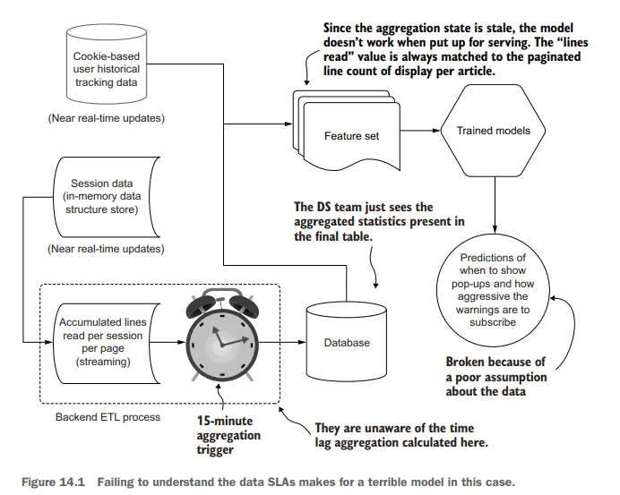
As an example of the dangers of a mere passing casual rendezvous with data being used for problem solving, let’s pretend that we both work at a content provider company. Because of the nature of the business model at our little company, our content is listed on the internet behind a timed paywall. For the first few articles that are read, no ads are shown, content is free to view, and the interaction experience is bereft of interruptions. After a set number of articles, an increasingly obnoxious series of pop-ups and disruptions are presented to coerce a subscription registration from the reader.

The prior state of the system was set by a basic heuristic controlled through the counting of article pages that the end user had seen. Realizing that this would potentially be off-putting for someone browsing during their first session on the platform, this was then adjusted to look at session length and an estimate of how many lines of each article had been read. As time went on, this seemingly simple rule set became so unwieldy and complex that the web team asked our DS team to build something that could predict on a per-user level the type and frequency of disruptions that would maximize subscription rates.

We spend a few months, mostly using the prior work that was built to support the heuristics approach, having the data engineering team create mirrored ETL processes of the data structures and manipulation logic that the frontend team has been using to generate decision data. With the data available in the data lake, we proceed to build a highly effective and accurate model that seems to perform exceptionally well on all of our holdout tests.

计算机代写|机器学习代写machine learning代考|Make sure you have the data

This example might seem a bit silly, but I’ve seen this situation play out dozens of times. Having an inability to get at the right data for model serving is a common problem.
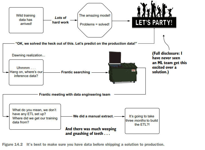
I’ve seen teams work with a manually extracted dataset (a one-time extract), build a truly remarkable solution with that data, and when ready to release the project to production, realize at the 11 th hour that the process for building that one-time extract required entirely manual actions by a DE team. The necessary data to make the solution effective was siloed off in a production infrastructure that the DS and DE teams had no ability to access. Figure 14.2 shows a rather familiar sight that I’ve borne witness to far too many times.

With no infrastructure present to bring the data into a usable form for predictions, as shown in figure 14.2, an entire project needs to be created for the DE team to build the ETL needed to materialize the data in a scheduled manner. Depending on the complexity of the data sources, this could take a while. Building hardened productiongrade ETL jobs that pull from multiple production relational databases and in-memory key-value stores is not a trivial reconciliation act, after all. Delays like this could lead (and have led) to project abandonment, regardless of the predictive capabilities of the DS portion of the solution.

This problem of complex ETL job creation becomes even more challenging if the predictions need to be conducted online. At that point, it’s not a question of the DE team working to get ETL processes running; rather, disparate groups in the engineering organization will have to accumulate the data into a single place in order to generate the collection of attributes that can be fed into a REST API request to the ML service.

This entire problem is solvable, though. During the time of EDA, the DS team should be evaluating the nature of the data generation, asking pointed questions to the data warehousing team:

  • Can the data be condensed to the fewest possible tables to reduce costs?
    -What is the team’s priority for fixing these sources if something breaks down?
  • Can I access this data from both the training and serving layers?
    -Will querying this data for serving meet the project SLA?
计算机代写|机器学习代写machine learning代考|COMP5328

机器学习代考

计算机代写|机器学习代写machine learning代考|Have you met your data?

我所说的会面,并不是在你传递数据、去续杯咖啡的路上,简短而礼貌地点头致意。也不是在展会上匆忙的30秒尴尬的自我介绍。相反,你应该与你的数据进行的会议更像是在一个安静、设备完善的地下酒吧里,喝着一瓶麦卡伦稀有酒桶(Macallan Rare Cask),进行长达数小时的私人谈话,分享见解,深入研究体现你们两人的细微差别,就像一杯又一杯柔滑的威士忌抚摸着你的消化道:真正真正地了解它。
提示:在编写一行代码之前,即使是为了进行实验,也要确保您拥有以最简单的方式(if/else语句)回答问题的基本性质所需的数据。如果你没有,看看你能不能得到它。如果你不能得到它,那就转向你能解决的问题。
为了说明与用于解决问题的数据仅仅是偶然相遇的危险,让我们假设我们都在一家内容提供商公司工作。由于我们这个小公司的商业模式的性质,我们的内容是在互联网上按时间收费的。对于阅读的前几篇文章,没有广告显示,内容可以自由查看,并且交互体验没有中断。在读完一定数量的文章后,会出现一系列令人讨厌的弹出窗口和干扰,迫使读者注册订阅。

系统的先验状态由一个基本的启发式设置,该启发式通过计算最终用户看过的文章页数来控制。意识到这可能会让那些在平台上的第一次浏览期间浏览的人感到不快,然后调整到查看会话长度和每篇文章的阅读行数估计。随着时间的推移,这个看似简单的规则集变得如此笨拙和复杂,以至于网络团队要求我们的DS团队构建一些东西,可以在每个用户的层面上预测中断的类型和频率,从而最大化订阅率。

我们花了几个月的时间,主要是使用之前为支持启发式方法而构建的工作,让数据工程团队创建数据结构和操作逻辑的镜像ETL流程,前端团队一直使用这些流程来生成决策数据。有了数据湖中可用的数据,我们继续构建一个非常有效和准确的模型,该模型似乎在我们所有的holdout测试中都表现得非常好。

计算机代写|机器学习代写machine learning代考|Make sure you have the data

这个例子可能看起来有点傻,但我已经看到这种情况发生过几十次了。无法为模型服务获取正确的数据是一个常见的问题。
我见过一些团队使用手动提取的数据集(一次性提取),使用该数据构建真正出色的解决方案,并在准备将项目发布到生产环境时,在第11个小时意识到构建一次性提取的过程完全需要DE团队的手动操作。使解决方案有效的必要数据被隔离在生产基础设施中,DS和DE团队无法访问这些数据。图14.2显示了一个相当熟悉的场景,我已经见过太多次了。

如图14.2所示,由于没有基础设施将数据转换为可用于预测的形式,因此需要为DE团队创建一个完整的项目,以构建以预定方式实现数据所需的ETL。根据数据源的复杂性,这可能需要一段时间。毕竟,构建从多个生产关系数据库和内存中的键值存储中提取的坚固的生产级ETL作业并不是一个微不足道的协调行为。不管解决方案的DS部分的预测能力如何,像这样的延迟可能导致(并且已经导致)项目放弃。

如果预测需要在线进行,那么复杂的ETL创造就业机会的问题就变得更具挑战性。在这一点上,这不是DE团队努力使ETL进程运行的问题;相反,工程组织中的不同组必须将数据积累到一个地方,以便生成可以提供给ML服务的REST API请求的属性集合。

不过,整个问题是可以解决的。在EDA期间,DS团队应该评估数据生成的性质,向数据仓库团队提出尖锐的问题:

能否将数据压缩到尽可能少的表中以降低成本?
-如果有东西坏了,团队修复这些源的首要任务是什么?

我可以从训练层和服务层访问这些数据吗?
-为服务而查询这些数据是否符合项目SLA?

计算机代写|机器学习代写machine learning代考 请认准statistics-lab™

统计代写请认准statistics-lab™. statistics-lab™为您的留学生涯保驾护航。

金融工程代写

金融工程是使用数学技术来解决金融问题。金融工程使用计算机科学、统计学、经济学和应用数学领域的工具和知识来解决当前的金融问题,以及设计新的和创新的金融产品。

非参数统计代写

非参数统计指的是一种统计方法,其中不假设数据来自于由少数参数决定的规定模型;这种模型的例子包括正态分布模型和线性回归模型。

广义线性模型代考

广义线性模型(GLM)归属统计学领域,是一种应用灵活的线性回归模型。该模型允许因变量的偏差分布有除了正态分布之外的其它分布。

术语 广义线性模型(GLM)通常是指给定连续和/或分类预测因素的连续响应变量的常规线性回归模型。它包括多元线性回归,以及方差分析和方差分析(仅含固定效应)。

有限元方法代写

有限元方法(FEM)是一种流行的方法,用于数值解决工程和数学建模中出现的微分方程。典型的问题领域包括结构分析、传热、流体流动、质量运输和电磁势等传统领域。

有限元是一种通用的数值方法,用于解决两个或三个空间变量的偏微分方程(即一些边界值问题)。为了解决一个问题,有限元将一个大系统细分为更小、更简单的部分,称为有限元。这是通过在空间维度上的特定空间离散化来实现的,它是通过构建对象的网格来实现的:用于求解的数值域,它有有限数量的点。边界值问题的有限元方法表述最终导致一个代数方程组。该方法在域上对未知函数进行逼近。[1] 然后将模拟这些有限元的简单方程组合成一个更大的方程系统,以模拟整个问题。然后,有限元通过变化微积分使相关的误差函数最小化来逼近一个解决方案。

tatistics-lab作为专业的留学生服务机构,多年来已为美国、英国、加拿大、澳洲等留学热门地的学生提供专业的学术服务,包括但不限于Essay代写,Assignment代写,Dissertation代写,Report代写,小组作业代写,Proposal代写,Paper代写,Presentation代写,计算机作业代写,论文修改和润色,网课代做,exam代考等等。写作范围涵盖高中,本科,研究生等海外留学全阶段,辐射金融,经济学,会计学,审计学,管理学等全球99%专业科目。写作团队既有专业英语母语作者,也有海外名校硕博留学生,每位写作老师都拥有过硬的语言能力,专业的学科背景和学术写作经验。我们承诺100%原创,100%专业,100%准时,100%满意。

随机分析代写


随机微积分是数学的一个分支,对随机过程进行操作。它允许为随机过程的积分定义一个关于随机过程的一致的积分理论。这个领域是由日本数学家伊藤清在第二次世界大战期间创建并开始的。

时间序列分析代写

随机过程,是依赖于参数的一组随机变量的全体,参数通常是时间。 随机变量是随机现象的数量表现,其时间序列是一组按照时间发生先后顺序进行排列的数据点序列。通常一组时间序列的时间间隔为一恒定值(如1秒,5分钟,12小时,7天,1年),因此时间序列可以作为离散时间数据进行分析处理。研究时间序列数据的意义在于现实中,往往需要研究某个事物其随时间发展变化的规律。这就需要通过研究该事物过去发展的历史记录,以得到其自身发展的规律。

回归分析代写

多元回归分析渐进(Multiple Regression Analysis Asymptotics)属于计量经济学领域,主要是一种数学上的统计分析方法,可以分析复杂情况下各影响因素的数学关系,在自然科学、社会和经济学等多个领域内应用广泛。

MATLAB代写

MATLAB 是一种用于技术计算的高性能语言。它将计算、可视化和编程集成在一个易于使用的环境中,其中问题和解决方案以熟悉的数学符号表示。典型用途包括:数学和计算算法开发建模、仿真和原型制作数据分析、探索和可视化科学和工程图形应用程序开发,包括图形用户界面构建MATLAB 是一个交互式系统,其基本数据元素是一个不需要维度的数组。这使您可以解决许多技术计算问题,尤其是那些具有矩阵和向量公式的问题,而只需用 C 或 Fortran 等标量非交互式语言编写程序所需的时间的一小部分。MATLAB 名称代表矩阵实验室。MATLAB 最初的编写目的是提供对由 LINPACK 和 EISPACK 项目开发的矩阵软件的轻松访问,这两个项目共同代表了矩阵计算软件的最新技术。MATLAB 经过多年的发展,得到了许多用户的投入。在大学环境中,它是数学、工程和科学入门和高级课程的标准教学工具。在工业领域,MATLAB 是高效研究、开发和分析的首选工具。MATLAB 具有一系列称为工具箱的特定于应用程序的解决方案。对于大多数 MATLAB 用户来说非常重要,工具箱允许您学习应用专业技术。工具箱是 MATLAB 函数(M 文件)的综合集合,可扩展 MATLAB 环境以解决特定类别的问题。可用工具箱的领域包括信号处理、控制系统、神经网络、模糊逻辑、小波、仿真等。

R语言代写问卷设计与分析代写
PYTHON代写回归分析与线性模型代写
MATLAB代写方差分析与试验设计代写
STATA代写机器学习/统计学习代写
SPSS代写计量经济学代写
EVIEWS代写时间序列分析代写
EXCEL代写深度学习代写
SQL代写各种数据建模与可视化代写

计算机代写|机器学习代写machine learning代考|Convex Optimization

如果你也在 怎样代写机器学习machine learning这个学科遇到相关的难题,请随时右上角联系我们的24/7代写客服。

机器学习(ML)是人工智能(AI)的一种类型,它允许软件应用程序在预测结果时变得更加准确,而无需明确编程。机器学习算法使用历史数据作为输入来预测新的输出值。

statistics-lab™ 为您的留学生涯保驾护航 在代写机器学习machine learning方面已经树立了自己的口碑, 保证靠谱, 高质且原创的统计Statistics代写服务。我们的专家在代写机器学习machine learning代写方面经验极为丰富,各种代写机器学习machine learning相关的作业也就用不着说。

我们提供的机器学习machine learning及其相关学科的代写,服务范围广, 其中包括但不限于:

  • Statistical Inference 统计推断
  • Statistical Computing 统计计算
  • Advanced Probability Theory 高等概率论
  • Advanced Mathematical Statistics 高等数理统计学
  • (Generalized) Linear Models 广义线性模型
  • Statistical Machine Learning 统计机器学习
  • Longitudinal Data Analysis 纵向数据分析
  • Foundations of Data Science 数据科学基础
计算机代写|机器学习代写machine learning代考|Convex Optimization

计算机代写|机器学习代写machine learning代考|Convex Optimization

When building a model in the context of machine learning, we often seek optimal model parameters $\boldsymbol{\theta}$, in the sense where they maximize the prior probability (or probability density) of predicting observed data. Here, we denote by $\tilde{f}(\theta)$ the target function we want to maximize. Optimal parameter values $\theta^{}$ are those that maximize the function $\hat{f}(\boldsymbol{\theta})$. $$ \boldsymbol{\theta}^{}=\underset{\boldsymbol{\theta}}{\arg \max } \tilde{f}(\boldsymbol{\theta}) .
$$
With a small caveat that will be covered below, convex optimization methods can be employed for the maximization task in equation 5.1. The key aspect of convex optimization methods is that, under certain conditions, they are guaranteed to reach optimal values for convex functions. Figure $5.1$ presents examples of convex and non-convex sets. For a set to be convex, you must be able to link any two points belonging to it without being outside of this set. Figure 5.1b presents a case where this property is not satisfied. For a convex function, the segment linking any pair of its points lies above or is equal to the function. Conversely, for a concave function, the opposite holds: the segment linking any pair of points lies below or is equal to the function. A concave function can be transformed into a convex one by taking the negative of it. Therefore, a maximization problem formulated as a concave optimization can be formulated in terms of a convex optimization following
$$
\boldsymbol{\theta}^{}=\underbrace{\underset{\theta}{\arg \max } \tilde{f}(\boldsymbol{\theta})}{\text {Concave optimization }} \equiv \underbrace{\arg \min -\tilde{f}(\boldsymbol{\theta})}{\text {Convex optimization }}
$$
In this chapter, we refer to convex optimization even if we are interested in maximizing a concave function, rather than minimizing a convex one. This choice is justified by the prevalence of convex optimization in the literature. Moreover, note that for several machine learning methods, we seek $\theta^{}$ based on a minimization problem where $-\tilde{f}(\boldsymbol{\theta})$ is a function of the difference between observed values and those predicted by a model. Figure $5.2$ presents examples of convex/concave and non-convex/non-concave functions. Nonconvex/non-concave functions such as the one in figure $5.2 \mathrm{~b}$ may have several local optima. Many functions of practical interest are non-convex/non-concave. As we will see in this chapter, convex optimization methods can also be employed for non-convex/nonconcave functions given that we choose a proper starting location. This chapter presents the gradient ascent and Newton-Raphson methods, as well as practical tools to be employed with them. For full-depth details regarding optimization methods, the reader should refer to dedicated textbooks. 1

计算机代写|机器学习代写machine learning代考|Gradient Ascent

A gradient is a vector containing the partial derivatives of a function with respect to its variables. For a continuous function, the maximum is located at the point where its gradient equals zero. Gradient ascent is based on the principle that as long as we move in the direction of the gradient, we are moving toward a maximum. For the unidimensional case, we choose to move to a new position by a scaling factor $\lambda$ times the derivative estimated at $\theta_{\text {old }}$,
$$
\theta_{\text {new }}=\theta_{\text {old }}+\underbrace{\lambda \cdot \tilde{f}^{\prime}\left(\theta_{\text {old }}\right)}{d} . $$ A common practice for setting $\lambda$ is to employ bachtracking line search where a new position is accepted if the Armijo rule ${ }^{2}$ is satisfied so that $$ \tilde{f}\left(\theta{\text {new }}\right) \geq \tilde{f}\left(\theta_{\text {old }}\right)+c \cdot d \tilde{f}^{\prime}\left(\theta_{\text {old }}\right) \text {, with } c \in(0,1) \text {. }
$$
Figure $5.3$ presents a comparison of the application of equation $5.2$ with the two extreme cases, $c=0$ and $c=1$. For $c=1, \theta_{\text {new }}$ is only accepted if $f\left(\theta_{\text {new }}\right)$ lies above the plane defined by the tangent at $\theta_{\text {old }}$. For $c=0, \theta_{\text {new }}$ is only accepted if $\tilde{f}\left(\theta_{\text {new }}\right)>\tilde{f}\left(\theta_{\text {old }}\right)$. The larger $c$ is, the stricter is the Armijo rule for ensuring that sufficient progress is made by the current step. With backtracking line search, we start from an initial value of $\lambda_{0}$ and reduce it until equation $5.2$ is satisfied. Algorithm 1 presents a minimal version of the gradient ascent with backtracking line search.

计算机代写|机器学习代写machine learning代考|Newton-Raphson

The Newton-Raphson method allows us to adaptively scale the search direction vector using the second-order derivative $\tilde{f}^{\prime \prime}(\theta)$. Knowing that the maximum of a function corresponds to the point where the gradient is zero, $\tilde{f}^{\prime}(\theta)=0$, we can find this maximum by formulating a linearized gradient equation using the second-order derivative of $\tilde{f}(\theta)$ and then set it equal to zero. The analytic formulation for the linearized gradient function (see \$3.4.2) approximated at the current location $\theta_{\text {old }}$ is
$$
\tilde{f}^{\prime}(\theta) \approx \tilde{f}^{\prime \prime}\left(\theta_{\text {old }}\right) \cdot\left(\theta-\theta_{\text {old }}\right)+\tilde{f}^{\prime \prime}\left(\theta_{\text {old }}\right)
$$
We can estimate $\theta_{\text {new }}$ by setting equation $5.3$ equal to zero, and then by solving for $\theta$, we obtain
$$
\theta_{\text {new }}=\theta_{\text {old }}-\frac{\tilde{f}^{\prime}\left(\theta_{\text {old }}\right)}{f^{\prime \prime}\left(\theta_{\text {old }}\right)}
$$
Let us consider the case where we want to find the maximum of a quadratic function (i.e., $\propto x^{2}$ ), as illustrated in figure 5.7. In the case of a quadratic function, the algorithm converges to the exact solution in one iteration, no matter the starting point, because the gradient of a quadratic function is exactly described by the linear function in equation $5.3$.

Algorithm 2 presents a minimal version of the Newton-Raphson method with backtracking line search. Note that at line 6 , there is again a scaling factor $\lambda$, which is employed because the NewtonRaphson method is exact only for quadratic functions. For more general non-convex/non-concave functions, the linearized gradient is an approximation such that a value of $\lambda=1$ will not always lead to a $\theta_{\text {new }}$ satisfying the Armijo rule in equation 5.2.
Figure $5.8$ presents the application of algorithm 2 to a nonconvex/non-concave function with an initial value $\theta_{0}=3.5$ and a scaling factor $\lambda_{0}=1$. For each loop, the pink solid line represents the linearized gradient function formulated in equation 5.3. Notice how, for the first two iterations, the second derivative $f^{\prime \prime}(\theta)>0$. Having a positive second derivative indicates that the linearization of $\tilde{f}^{\prime}(\theta)$ equals zero for a minimum rather than for a maximum. One simple option in this situation is to define $\lambda=-\lambda$ in order to ensure that the next slep moves in the same dirextion as the gradient. The convergence with Newton-Raphson is typically faster than with gradient ascent.

计算机代写|机器学习代写machine learning代考|Convex Optimization

机器学习代考

计算机代写|机器学习代写machine learning代考|Convex Optimization

在机器学习的背景下构建模型时,我们经常寻求最优的模型参数θ,在它们最大化预测观察数据的先验概率(或概率密度)的意义上。在这里,我们表示F~(θ)我们想要最大化的目标函数。最佳参数值θ是最大化功能的那些F^(θ).

θ=参数⁡最大限度θF~(θ).
有一点将在下面介绍,凸优化方法可以用于方程 5.1 中的最大化任务。凸优化方法的关键在于,在某些条件下,它们保证达到凸函数的最优值。数字5.1给出了凸集和非凸集的例子。对于一个凸集,您必须能够链接属于它的任何两个点,而不会超出该集。图 5.1b 展示了一个不满足此属性的情况。对于凸函数,连接其任意一对点的线段位于该函数之上或等于该函数。相反,对于凹函数,相反的情况成立:连接任何一对点的线段位于该函数的下方或等于该函数。一个凹函数可以通过取负数转换为一个凸函数。因此,一个被表述为凹优化的最大化问题可以被表述为以下的凸优化

θ=参数⁡最大限度θF~(θ)⏟凹优化 ≡参数⁡分钟−F~(θ)⏟凸优化 
在本章中,即使我们对最大化凹函数而不是最小化凸函数感兴趣,我们也会提到凸优化。文献中凸优化的普遍性证明了这种选择是合理的。此外,请注意,对于几种机器学习方法,我们寻求θ基于最小化问题,其中−F~(θ)是观测值与模型预测值之间差异的函数。数字5.2给出了凸/凹和非凸/非凹函数的例子。非凸/非凹函数,如图所示5.2 b可能有几个局部最优值。许多实际感兴趣的函数是非凸/非凹的。正如我们将在本章中看到的,如果我们选择了合适的起始位置,凸优化方法也可以用于非凸/非凹函数。本章介绍梯度上升法和 Newton-Raphson 方法,以及与它们一起使用的实用工具。有关优化方法的详细信息,读者应参考专门的教科书。1

计算机代写|机器学习代写machine learning代考|Gradient Ascent

梯度是包含函数相对于其变量的偏导数的向量。对于连续函数,最大值位于其梯度为零的点。梯度上升是基于这样的原理,只要我们沿着梯度的方向移动,我们就会朝着一个最大值移动。对于一维情况,我们选择按比例因子移动到新位置λ乘以估计的导数θ老的 ,

θ新的 =θ老的 +λ⋅F~′(θ老的 )⏟d.设置的常见做法λ是采用 bachtracking 线搜索,如果 Armijo 规则接受新位置2满足,使得

F~(θ新的 )≥F~(θ老的 )+C⋅dF~′(θ老的 ), 和 C∈(0,1). 
数字5.3比较了方程的应用5.2在两种极端情况下,C=0和C=1. 为了C=1,θ新的 仅在以下情况下被接受F(θ新的 )位于由切线定义的平面之上θ老的 . 为了C=0,θ新的 仅在以下情况下被接受F~(θ新的 )>F~(θ老的 ). 较大的C也就是说,更严格的是确保当前步骤取得足够进展的 Armijo 规则。通过回溯线搜索,我们从初始值开始λ0并减少它直到方程5.2很满意。算法 1 提出了带有回溯线搜索的梯度上升的最小版本。

计算机代写|机器学习代写machine learning代考|Newton-Raphson

Newton-Raphson 方法允许我们使用二阶导数自适应地缩放搜索方向向量F~′′(θ). 知道函数的最大值对应于梯度为零的点,F~′(θ)=0,我们可以通过使用的二阶导数制定线性梯度方程来找到这个最大值F~(θ)然后将其设置为零。在当前位置近似的线性化梯度函数的解析公式(见$ 3.4.2)θ老的 是

F~′(θ)≈F~′′(θ老的 )⋅(θ−θ老的 )+F~′′(θ老的 )
我们可以估计θ新的 通过设置方程5.3等于零,然后通过求解θ, 我们获得

θ新的 =θ老的 −F~′(θ老的 )F′′(θ老的 )
让我们考虑一下我们想要找到二次函数的最大值的情况(即,∝X2),如图 5.7 所示。在二次函数的情况下,算法在一次迭代中收敛到精确解,无论起点如何,因为二次函数的梯度精确地由方程中的线性函数描述5.3.

算法 2 提供了带有回溯线搜索的 Newton-Raphson 方法的最小版本。请注意,在第 6 行,还有一个比例因子λ,这是因为 NewtonRaphson 方法仅适用于二次函数。对于更一般的非凸/非凹函数,线性化梯度是一个近似值,使得λ=1不会总是导致θ新的 满足方程 5.2 中的 Armijo 规则。
数字5.8将算法 2 应用于具有初始值的非凸/非凹函数θ0=3.5和比例因子λ0=1. 对于每个循环,粉红色实线表示方程 5.3 中公式化的线性梯度函数。请注意,对于前两次迭代,二阶导数F′′(θ)>0. 具有正二阶导数表示线性化F~′(θ)最小值等于 0,而不是最大值。在这种情况下,一个简单的选择是定义λ=−λ为了确保下一个 slep 在与梯度相同的方向上移动。与 Newton-Raphson 的收敛通常比梯度上升更快。

计算机代写|机器学习代写machine learning代考 请认准statistics-lab™

统计代写请认准statistics-lab™. statistics-lab™为您的留学生涯保驾护航。

金融工程代写

金融工程是使用数学技术来解决金融问题。金融工程使用计算机科学、统计学、经济学和应用数学领域的工具和知识来解决当前的金融问题,以及设计新的和创新的金融产品。

非参数统计代写

非参数统计指的是一种统计方法,其中不假设数据来自于由少数参数决定的规定模型;这种模型的例子包括正态分布模型和线性回归模型。

广义线性模型代考

广义线性模型(GLM)归属统计学领域,是一种应用灵活的线性回归模型。该模型允许因变量的偏差分布有除了正态分布之外的其它分布。

术语 广义线性模型(GLM)通常是指给定连续和/或分类预测因素的连续响应变量的常规线性回归模型。它包括多元线性回归,以及方差分析和方差分析(仅含固定效应)。

有限元方法代写

有限元方法(FEM)是一种流行的方法,用于数值解决工程和数学建模中出现的微分方程。典型的问题领域包括结构分析、传热、流体流动、质量运输和电磁势等传统领域。

有限元是一种通用的数值方法,用于解决两个或三个空间变量的偏微分方程(即一些边界值问题)。为了解决一个问题,有限元将一个大系统细分为更小、更简单的部分,称为有限元。这是通过在空间维度上的特定空间离散化来实现的,它是通过构建对象的网格来实现的:用于求解的数值域,它有有限数量的点。边界值问题的有限元方法表述最终导致一个代数方程组。该方法在域上对未知函数进行逼近。[1] 然后将模拟这些有限元的简单方程组合成一个更大的方程系统,以模拟整个问题。然后,有限元通过变化微积分使相关的误差函数最小化来逼近一个解决方案。

tatistics-lab作为专业的留学生服务机构,多年来已为美国、英国、加拿大、澳洲等留学热门地的学生提供专业的学术服务,包括但不限于Essay代写,Assignment代写,Dissertation代写,Report代写,小组作业代写,Proposal代写,Paper代写,Presentation代写,计算机作业代写,论文修改和润色,网课代做,exam代考等等。写作范围涵盖高中,本科,研究生等海外留学全阶段,辐射金融,经济学,会计学,审计学,管理学等全球99%专业科目。写作团队既有专业英语母语作者,也有海外名校硕博留学生,每位写作老师都拥有过硬的语言能力,专业的学科背景和学术写作经验。我们承诺100%原创,100%专业,100%准时,100%满意。

随机分析代写


随机微积分是数学的一个分支,对随机过程进行操作。它允许为随机过程的积分定义一个关于随机过程的一致的积分理论。这个领域是由日本数学家伊藤清在第二次世界大战期间创建并开始的。

时间序列分析代写

随机过程,是依赖于参数的一组随机变量的全体,参数通常是时间。 随机变量是随机现象的数量表现,其时间序列是一组按照时间发生先后顺序进行排列的数据点序列。通常一组时间序列的时间间隔为一恒定值(如1秒,5分钟,12小时,7天,1年),因此时间序列可以作为离散时间数据进行分析处理。研究时间序列数据的意义在于现实中,往往需要研究某个事物其随时间发展变化的规律。这就需要通过研究该事物过去发展的历史记录,以得到其自身发展的规律。

回归分析代写

多元回归分析渐进(Multiple Regression Analysis Asymptotics)属于计量经济学领域,主要是一种数学上的统计分析方法,可以分析复杂情况下各影响因素的数学关系,在自然科学、社会和经济学等多个领域内应用广泛。

MATLAB代写

MATLAB 是一种用于技术计算的高性能语言。它将计算、可视化和编程集成在一个易于使用的环境中,其中问题和解决方案以熟悉的数学符号表示。典型用途包括:数学和计算算法开发建模、仿真和原型制作数据分析、探索和可视化科学和工程图形应用程序开发,包括图形用户界面构建MATLAB 是一个交互式系统,其基本数据元素是一个不需要维度的数组。这使您可以解决许多技术计算问题,尤其是那些具有矩阵和向量公式的问题,而只需用 C 或 Fortran 等标量非交互式语言编写程序所需的时间的一小部分。MATLAB 名称代表矩阵实验室。MATLAB 最初的编写目的是提供对由 LINPACK 和 EISPACK 项目开发的矩阵软件的轻松访问,这两个项目共同代表了矩阵计算软件的最新技术。MATLAB 经过多年的发展,得到了许多用户的投入。在大学环境中,它是数学、工程和科学入门和高级课程的标准教学工具。在工业领域,MATLAB 是高效研究、开发和分析的首选工具。MATLAB 具有一系列称为工具箱的特定于应用程序的解决方案。对于大多数 MATLAB 用户来说非常重要,工具箱允许您学习应用专业技术。工具箱是 MATLAB 函数(M 文件)的综合集合,可扩展 MATLAB 环境以解决特定类别的问题。可用工具箱的领域包括信号处理、控制系统、神经网络、模糊逻辑、小波、仿真等。

R语言代写问卷设计与分析代写
PYTHON代写回归分析与线性模型代写
MATLAB代写方差分析与试验设计代写
STATA代写机器学习/统计学习代写
SPSS代写计量经济学代写
EVIEWS代写时间序列分析代写
EXCEL代写深度学习代写
SQL代写各种数据建模与可视化代写

计算机代写|机器学习代写machine learning代考|Log-Normal Distribution

如果你也在 怎样代写机器学习machine learning这个学科遇到相关的难题,请随时右上角联系我们的24/7代写客服。

机器学习(ML)是人工智能(AI)的一种类型,它允许软件应用程序在预测结果时变得更加准确,而无需明确编程。机器学习算法使用历史数据作为输入来预测新的输出值。

statistics-lab™ 为您的留学生涯保驾护航 在代写机器学习machine learning方面已经树立了自己的口碑, 保证靠谱, 高质且原创的统计Statistics代写服务。我们的专家在代写机器学习machine learning代写方面经验极为丰富,各种代写机器学习machine learning相关的作业也就用不着说。

我们提供的机器学习machine learning及其相关学科的代写,服务范围广, 其中包括但不限于:

  • Statistical Inference 统计推断
  • Statistical Computing 统计计算
  • Advanced Probability Theory 高等概率论
  • Advanced Mathematical Statistics 高等数理统计学
  • (Generalized) Linear Models 广义线性模型
  • Statistical Machine Learning 统计机器学习
  • Longitudinal Data Analysis 纵向数据分析
  • Foundations of Data Science 数据科学基础
计算机代写|机器学习代写machine learning代考|Log-Normal Distribution

计算机代写|机器学习代写machine learning代考|Multivariate Log-Normal

$X_{1}, X_{2}, \cdots, X_{n}$ are jointly log-normal if $\ln X_{1}, \ln X_{2}, \cdots, \ln X_{n}$ are $\quad \mathbf{x} \in\left(\mathbb{R}^{+}\right)^{n}: \mathbf{x} \sim \ln \mathcal{N}\left(\mathbf{x} ; \mu_{\ln } \mathbf{x}, \mathbf{\Sigma}{\ln \mathbf{x}}\right.$ jointly Normal. The multivariate log-normal PDF is parameterized by the mean values $\left(\mu{\ln X_{i}}=\lambda\right)$, variances $\left(\sigma_{\ln X_{i}}^{2}=\zeta^{2}\right)$, and
correlation coefficients $\left(\rho_{\mathrm{n}} X_{i} \ln X_{j}\right)$ defined in the log-transformed
space. Correlation coefficients in the $\log$-space $\rho_{\ln } x_{i} \ln X_{j}$ are related
to the correlation coefficients in the original space $\rho X_{i} x_{j}$ using the relation
$$
\rho_{\ln X_{i}} \ln X_{j}=\frac{1}{\zeta_{i} \zeta_{j}} \ln \left(1+\rho_{X_{i} X_{j}} \delta_{X_{1}} \delta_{X_{j}}\right)
$$
where $\rho_{\ln X_{i} \ln X_{j}} \approx \rho_{X_{i} X_{j}}$ for $\delta_{X_{i}}, \delta_{X_{j}} \ll 0.3$. The PDF for two random variables $\left{X_{1}, X_{2}\right}$ such that $\left{x_{1}, x_{2}\right}>0$ is
$$
f_{X_{1} X_{2}}\left(x_{1}, x_{2}\right)=\frac{1}{x_{1} x_{2} \sqrt{2 \pi} \zeta_{1} \zeta_{2} \sqrt{1-\rho_{\mathrm{ln}}^{2}}} \exp \left(-\frac{1}{2\left(1-\rho_{\mathrm{ln}}^{2}\right)}\left(\left(\frac{\ln x_{1}-\lambda_{1}}{\zeta_{1}}\right)^{2}+\left(\frac{\ln x_{2}-\lambda_{2}}{\zeta_{2}}\right)^{2}-2 \rho_{\mathrm{n}}\left(\frac{\ln x_{1}-\lambda_{1}}{\zeta_{1}}\right)\left(\frac{\ln x_{2}-\lambda_{2}}{\zeta_{2}}\right)^{2}\right)\right)
$$

Figure $4.10$ presents an example of bivariate log-normal PDF with parameters $\mu_{1}=\mu_{2}=1.5, \sigma_{1}=\sigma_{2}=0.5$, and $\rho=0.9$. The general formulation for the multivariate log-normal PDF is
$$
\begin{aligned}
f_{\mathbf{X}}(\mathbf{x}) &=\ln \mathcal{N}\left(\mathbf{x} ; \boldsymbol{\mu}{\ln \mathbf{X}}, \boldsymbol{\Sigma}{\ln \mathbf{x}}\right) \
&=\frac{1}{\left(\Pi_{i=1}^{n} x_{i}\right)(2 \pi)^{n / 2}\left(\operatorname{det} \boldsymbol{\Sigma}{\mathbf{n} \mathbf{X}}\right)^{1 / 2}} \exp \left(-\frac{1}{2}\left(\ln \mathbf{x}-\boldsymbol{\mu}{\ln \mathbf{x}}\right)^{\top} \boldsymbol{\Sigma}{\ln \mathbf{X}}^{-1}\left(\ln \mathbf{x}-\boldsymbol{\mu}{\ln \mathbf{x}}\right)\right)
\end{aligned}
$$
where $\boldsymbol{\mu} \ln \mathbf{x}$ and $\boldsymbol{\Sigma}_{\ln \mathbf{x}}$ are respectively the mean vector and covariance matrix defined in the log-space.

计算机代写|机器学习代写machine learning代考|Properties

Because the log-normal distribution is obtained through a transformation of the Normal distribution, it inherits several of its properties. $\operatorname{matrix} \Sigma_{\mathrm{ln} \mathbf{X}}$.

  1. Its marginal distributions are also log-normal, and the PDF of any marginal is given by
    $$
    x_{i}: X_{i} \sim \ln \mathcal{N}\left(x_{i} ;\left[\boldsymbol{\mu}{\ln } \mathbf{x}\right]{i+}\left[\boldsymbol{\Sigma}{\ln \mathbf{x}}\right]{i i}\right) .
    $$
  2. The absence of correlation implies statistical independence Remember that this is not generally true for other types of random variables (see $\S 3.3 .5$ ),
    $$
    \rho_{i j}=0 \Leftrightarrow X_{i} \perp X_{j}
    $$
  3. Conditional distributions are log-normal, so the $\mathrm{PDF}$ of $\mathbf{X}{i}$ given an observation $\mathbf{X}{j}=\mathbf{x}{j}$ is given by $$ f \mathbf{X}{i} \mid \mathbf{x}{j}(\mathbf{x}{i} \mid \underbrace{\mathbf{X}{j}=\mathbf{x}{j}}{\text {observations }})=\ln \mathcal{N}\left(\mathbf{x}{i} ; \boldsymbol{\mu}{\ln i \mid j}, \mathbf{\Sigma}{\ln i \mid j}\right)+
    $$
    where the conditional mean vector and covariance are
    $$
    \begin{aligned}
    &\boldsymbol{\mu}{\ln i \mid j}=\mu{n i}+\Sigma_{\ln i j} \Sigma_{j}^{-1}\left(\ln \mathbf{x}{j}-\mu{\ln j}\right) \
    &\Sigma_{\ln i \mid j}=\Sigma_{\ln i}-\Sigma_{\ln i j} \Sigma_{j}^{-1} \Sigma_{\ln i j}^{\top}
    \end{aligned}
    $$
  4. The multiplication of jointly log-normal random variables is jointly $\log$-normal so that for $X \sim \ln \mathcal{N}\left(x ; \lambda_{X}, \zeta_{X}\right)$ and $Y \sim$ $\ln \mathcal{N}\left(y ; \lambda_{Y}, \zeta_{Y}\right)$, where $X \perp Y$,
    $$
    \left.\begin{array}{rl}
    Z & =X \cdot Y \
    \sim & \ln \mathcal{N}\left(z ; \lambda_{Z}, \zeta_{Z}\right)
    \end{array}\right} \begin{aligned}
    &\lambda_{Z}=\lambda_{X}+\lambda_{Y} \
    &\zeta_{Z}^{2}=\zeta_{X}^{2}+\zeta_{Y}^{2}
    \end{aligned}
    $$
    Because the product of log-normal random variables can be transformed in the sum of Normal random variables, the properties of the central limit theorem presented in $\S 4.1 .3$ still hold.

计算机代写|机器学习代写machine learning代考|Beta Distribution

The Beta distribution is defined over the interval $(0,1)$. It can be scaled by the transformation $x^{\prime}=x \cdot(b-a)+a$ to model bounded quantities within any range $(a, b)$. The Beta probability density function (PDF) is defined by
$$
f_{X}(x)=\mathcal{B}(x ; \alpha, \beta)=\frac{x^{\alpha-1}(1-x)^{\beta-1}}{\mathrm{~B}(\alpha, \beta)}\left{\begin{array}{l}
\alpha>0 \
\beta>0 \
\mathrm{~B}(\alpha, \beta): \text { Beta function }
\end{array}\right.
$$
where $\alpha$ and $\beta$ are the two distribution parameters, and the Beta function $\mathrm{B}(\alpha, \beta)$ is the normalization constant so that
$$
\mathrm{B}(\alpha, \beta)=\int_{0}^{1} x^{\alpha-1}(1-x)^{\beta-1} d x
$$
A common application of the Beta PDF is to employ the interval $(0,1)$ to model the probability density of a probability itself. Let us consider two mutually exclusive and collectively exhaustive events, for example, any event $A$ and its complement $\bar{A}, \mathcal{S}={A, \bar{A}}$. If the probability that the event $A$ occurs is uncertain, it can be described by a random variable so that
$$
\left{\begin{array}{l}
\operatorname{Pr}(A)=X \
\operatorname{Pr}(A)=1-X
\end{array}\right.
$$
where $x \in(0,1): X \sim \mathcal{B}(x ; \alpha, \beta)$. The parameter $\alpha$ can be interpreted as pseudo-counts representing the number of observations of the event $A$, and $\beta$ is the number of observations of the complementary event $\bar{A}$. This relation between pseudo-counts and the Beta distribution, as well as practical applications, are further detailed in chapter 6. Figure $4.11$ presents examples of Beta PDFs for three sets of parameters. Note how for $\alpha=\beta=1$, the Beta distribution is analogous to the Uniform distribution $\mathcal{U}(x ; 0,1)$.

计算机代写|机器学习代写machine learning代考|Log-Normal Distribution

机器学习代考

计算机代写|机器学习代写machine learning代考|Multivariate Log-Normal

X1,X2,⋯,Xn是联合对数正态如果ln⁡X1,ln⁡X2,⋯,ln⁡Xn是X∈(R+)n:X∼ln⁡ñ(X;μlnX,Σln⁡X联合正常。多元对数正态 PDF 由平均值参数化(μln⁡X一世=λ), 方差(σln⁡X一世2=G2), 和
相关系数(ρnX一世ln⁡Xj)在对数变换
空间中定义。相关系数日志-空间ρlnX一世ln⁡Xj与
原始空间中的相关系数有关ρX一世Xj使用关系

ρln⁡X一世ln⁡Xj=1G一世Gjln⁡(1+ρX一世XjdX1dXj)
在哪里ρln⁡X一世ln⁡Xj≈ρX一世Xj为了dX一世,dXj≪0.3. 两个随机变量的 PDF\left{X_{1}, X_{2}\right}\left{X_{1}, X_{2}\right}这样\left{x_{1}, x_{2}\right}>0\left{x_{1}, x_{2}\right}>0是

FX1X2(X1,X2)=1X1X22圆周率G1G21−ρln2经验⁡(−12(1−ρln2)((ln⁡X1−λ1G1)2+(ln⁡X2−λ2G2)2−2ρn(ln⁡X1−λ1G1)(ln⁡X2−λ2G2)2))

数字4.10给出了一个带参数的双变量对数正态 PDF 示例μ1=μ2=1.5,σ1=σ2=0.5, 和ρ=0.9. 多元对数正态 PDF 的一般公式是

FX(X)=ln⁡ñ(X;μln⁡X,Σln⁡X) =1(圆周率一世=1nX一世)(2圆周率)n/2(这⁡ΣnX)1/2经验⁡(−12(ln⁡X−μln⁡X)⊤Σln⁡X−1(ln⁡X−μln⁡X))
在哪里μln⁡X和Σln⁡X分别是在对数空间中定义的平均向量和协方差矩阵。

计算机代写|机器学习代写machine learning代考|Properties

因为对数正态分布是通过正态分布的变换获得的,所以它继承了它的几个属性。矩阵⁡ΣlnX.

  1. 它的边际分布也是对数正态分布,任何边际的 PDF 由下式给出
    X一世:X一世∼ln⁡ñ(X一世;[μlnX]一世+[Σln⁡X]一世一世).
  2. 缺乏相关性意味着统计独立性 请记住,对于其他类型的随机变量,这通常不是正确的(参见§§3.3.5 ),
    ρ一世j=0⇔X一世⊥Xj
  3. 条件分布是对数正态分布,所以磷DF的X一世给予观察Xj=Xj是(谁)给的FX一世∣Xj(X一世∣Xj=Xj⏟观察 )=ln⁡ñ(X一世;μln⁡一世∣j,Σln⁡一世∣j)+
    其中条件均值向量和协方差是
    μln⁡一世∣j=μn一世+Σln⁡一世jΣj−1(ln⁡Xj−μln⁡j) Σln⁡一世∣j=Σln⁡一世−Σln⁡一世jΣj−1Σln⁡一世j⊤
  4. 联合对数正态随机变量的乘法是联合日志-正常,因此对于X∼ln⁡ñ(X;λX,GX)和是∼ ln⁡ñ(是;λ是,G是), 在哪里X⊥是,
    \left.\begin{array}{rl} Z & =X \cdot Y \ \sim & \ln \mathcal{N}\left(z ; \lambda_{Z}, \zeta_{Z}\right) \end {数组}\right} \begin{aligned} &\lambda_{Z}=\lambda_{X}+\lambda_{Y} \ &\zeta_{Z}^{2}=\zeta_{X}^{2} +\zeta_{Y}^{2} \end{对齐}\left.\begin{array}{rl} Z & =X \cdot Y \ \sim & \ln \mathcal{N}\left(z ; \lambda_{Z}, \zeta_{Z}\right) \end {数组}\right} \begin{aligned} &\lambda_{Z}=\lambda_{X}+\lambda_{Y} \ &\zeta_{Z}^{2}=\zeta_{X}^{2} +\zeta_{Y}^{2} \end{对齐}
    因为对数正态随机变量的乘积可以转化为正态随机变量之和,所以中心极限定理的性质§§4.1.3仍然持有。

计算机代写|机器学习代写machine learning代考|Beta Distribution

Beta 分布在区间上定义(0,1). 它可以通过变换进行缩放X′=X⋅(b−一个)+一个对任何范围内的有界数量进行建模(一个,b). Beta 概率密度函数 (PDF) 由
$$
f_{X}(x)=\mathcal{B}(x ; \alpha, \beta)=\frac{x^{\alpha-1}(1- x)^{\beta-1}}{\mathrm{~B}(\alpha, \beta)}\left{

一个>0 b>0  乙(一个,b): 贝塔函数 \正确的。

在H和r和$一个$一个nd$b$一个r和吨H和吨在○d一世s吨r一世b在吨一世○np一个r一个米和吨和rs,一个nd吨H和乙和吨一个F在nC吨一世○n$乙(一个,b)$一世s吨H和n○r米一个l一世和一个吨一世○nC○ns吨一个n吨s○吨H一个吨
\mathrm{B}(\alpha, \beta)=\int_{0}^{1} x^{\alpha-1}(1-x)^{\beta-1} dx

一个C○米米○n一个ppl一世C一个吨一世○n○F吨H和乙和吨一个磷DF一世s吨○和米pl○是吨H和一世n吨和r在一个l$(0,1)$吨○米○d和l吨H和pr○b一个b一世l一世吨是d和ns一世吨是○F一个pr○b一个b一世l一世吨是一世吨s和lF.大号和吨在sC○ns一世d和r吨在○米在吨在一个ll是和XCl在s一世在和一个ndC○ll和C吨一世在和l是和XH一个在s吨一世在和和在和n吨s,F○r和X一个米pl和,一个n是和在和n吨$一个$一个nd一世吨sC○米pl和米和n吨$一个¯,小号=一个,一个¯$.我F吨H和pr○b一个b一世l一世吨是吨H一个吨吨H和和在和n吨$一个$○CC在rs一世s在nC和r吨一个一世n,一世吨C一个nb和d和sCr一世b和db是一个r一个nd○米在一个r一世一个bl和s○吨H一个吨
\剩下{

公关⁡(一个)=X 公关⁡(一个)=1−X\正确的。
$$
在哪里X∈(0,1):X∼乙(X;一个,b). 参数一个可以解释为表示事件观察次数的伪计数一个, 和b是互补事件的观察次数一个¯. 伪计数与 Beta 分布之间的这种关系以及实际应用将在第 6 章中进一步详述。4.11提供了三组参数的 Beta PDF 示例。注意如何为一个=b=1, Beta 分布类似于均匀分布在(X;0,1).

计算机代写|机器学习代写machine learning代考 请认准statistics-lab™

统计代写请认准statistics-lab™. statistics-lab™为您的留学生涯保驾护航。

金融工程代写

金融工程是使用数学技术来解决金融问题。金融工程使用计算机科学、统计学、经济学和应用数学领域的工具和知识来解决当前的金融问题,以及设计新的和创新的金融产品。

非参数统计代写

非参数统计指的是一种统计方法,其中不假设数据来自于由少数参数决定的规定模型;这种模型的例子包括正态分布模型和线性回归模型。

广义线性模型代考

广义线性模型(GLM)归属统计学领域,是一种应用灵活的线性回归模型。该模型允许因变量的偏差分布有除了正态分布之外的其它分布。

术语 广义线性模型(GLM)通常是指给定连续和/或分类预测因素的连续响应变量的常规线性回归模型。它包括多元线性回归,以及方差分析和方差分析(仅含固定效应)。

有限元方法代写

有限元方法(FEM)是一种流行的方法,用于数值解决工程和数学建模中出现的微分方程。典型的问题领域包括结构分析、传热、流体流动、质量运输和电磁势等传统领域。

有限元是一种通用的数值方法,用于解决两个或三个空间变量的偏微分方程(即一些边界值问题)。为了解决一个问题,有限元将一个大系统细分为更小、更简单的部分,称为有限元。这是通过在空间维度上的特定空间离散化来实现的,它是通过构建对象的网格来实现的:用于求解的数值域,它有有限数量的点。边界值问题的有限元方法表述最终导致一个代数方程组。该方法在域上对未知函数进行逼近。[1] 然后将模拟这些有限元的简单方程组合成一个更大的方程系统,以模拟整个问题。然后,有限元通过变化微积分使相关的误差函数最小化来逼近一个解决方案。

tatistics-lab作为专业的留学生服务机构,多年来已为美国、英国、加拿大、澳洲等留学热门地的学生提供专业的学术服务,包括但不限于Essay代写,Assignment代写,Dissertation代写,Report代写,小组作业代写,Proposal代写,Paper代写,Presentation代写,计算机作业代写,论文修改和润色,网课代做,exam代考等等。写作范围涵盖高中,本科,研究生等海外留学全阶段,辐射金融,经济学,会计学,审计学,管理学等全球99%专业科目。写作团队既有专业英语母语作者,也有海外名校硕博留学生,每位写作老师都拥有过硬的语言能力,专业的学科背景和学术写作经验。我们承诺100%原创,100%专业,100%准时,100%满意。

随机分析代写


随机微积分是数学的一个分支,对随机过程进行操作。它允许为随机过程的积分定义一个关于随机过程的一致的积分理论。这个领域是由日本数学家伊藤清在第二次世界大战期间创建并开始的。

时间序列分析代写

随机过程,是依赖于参数的一组随机变量的全体,参数通常是时间。 随机变量是随机现象的数量表现,其时间序列是一组按照时间发生先后顺序进行排列的数据点序列。通常一组时间序列的时间间隔为一恒定值(如1秒,5分钟,12小时,7天,1年),因此时间序列可以作为离散时间数据进行分析处理。研究时间序列数据的意义在于现实中,往往需要研究某个事物其随时间发展变化的规律。这就需要通过研究该事物过去发展的历史记录,以得到其自身发展的规律。

回归分析代写

多元回归分析渐进(Multiple Regression Analysis Asymptotics)属于计量经济学领域,主要是一种数学上的统计分析方法,可以分析复杂情况下各影响因素的数学关系,在自然科学、社会和经济学等多个领域内应用广泛。

MATLAB代写

MATLAB 是一种用于技术计算的高性能语言。它将计算、可视化和编程集成在一个易于使用的环境中,其中问题和解决方案以熟悉的数学符号表示。典型用途包括:数学和计算算法开发建模、仿真和原型制作数据分析、探索和可视化科学和工程图形应用程序开发,包括图形用户界面构建MATLAB 是一个交互式系统,其基本数据元素是一个不需要维度的数组。这使您可以解决许多技术计算问题,尤其是那些具有矩阵和向量公式的问题,而只需用 C 或 Fortran 等标量非交互式语言编写程序所需的时间的一小部分。MATLAB 名称代表矩阵实验室。MATLAB 最初的编写目的是提供对由 LINPACK 和 EISPACK 项目开发的矩阵软件的轻松访问,这两个项目共同代表了矩阵计算软件的最新技术。MATLAB 经过多年的发展,得到了许多用户的投入。在大学环境中,它是数学、工程和科学入门和高级课程的标准教学工具。在工业领域,MATLAB 是高效研究、开发和分析的首选工具。MATLAB 具有一系列称为工具箱的特定于应用程序的解决方案。对于大多数 MATLAB 用户来说非常重要,工具箱允许您学习应用专业技术。工具箱是 MATLAB 函数(M 文件)的综合集合,可扩展 MATLAB 环境以解决特定类别的问题。可用工具箱的领域包括信号处理、控制系统、神经网络、模糊逻辑、小波、仿真等。

R语言代写问卷设计与分析代写
PYTHON代写回归分析与线性模型代写
MATLAB代写方差分析与试验设计代写
STATA代写机器学习/统计学习代写
SPSS代写计量经济学代写
EVIEWS代写时间序列分析代写
EXCEL代写深度学习代写
SQL代写各种数据建模与可视化代写

计算机代写|机器学习代写machine learning代考|Conditional Distributions

如果你也在 怎样代写机器学习machine learning这个学科遇到相关的难题,请随时右上角联系我们的24/7代写客服。

机器学习(ML)是人工智能(AI)的一种类型,它允许软件应用程序在预测结果时变得更加准确,而无需明确编程。机器学习算法使用历史数据作为输入来预测新的输出值。

statistics-lab™ 为您的留学生涯保驾护航 在代写机器学习machine learning方面已经树立了自己的口碑, 保证靠谱, 高质且原创的统计Statistics代写服务。我们的专家在代写机器学习machine learning代写方面经验极为丰富,各种代写机器学习machine learning相关的作业也就用不着说。

我们提供的机器学习machine learning及其相关学科的代写,服务范围广, 其中包括但不限于:

  • Statistical Inference 统计推断
  • Statistical Computing 统计计算
  • Advanced Probability Theory 高等概率论
  • Advanced Mathematical Statistics 高等数理统计学
  • (Generalized) Linear Models 广义线性模型
  • Statistical Machine Learning 统计机器学习
  • Longitudinal Data Analysis 纵向数据分析
  • Foundations of Data Science 数据科学基础
计算机代写|机器学习代写machine learning代考|Conditional Distributions

计算机代写|机器学习代写machine learning代考|Conditional Distributions

For the beam example illustrated in figure 4.5, our prior knowledge for the resistance $\left{X_{1}, X_{2}\right}$ of two adjacent beams is
and we know that the beam resistances are correlated with $\rho_{12}=$ 0.8. Such a correlation could arise because both beams were fabricated with the same process, in the same factory. This prior knowledge is described by the joint bivariate Normal PDF,
$$
f_{X_{1} X_{2}}\left(x_{1}, x_{2}\right)=\mathcal{N}\left(\mathbf{x} ; \boldsymbol{\mu}{\mathbf{X}}, \mathbf{\Sigma}{\mathbf{X}}\right)\left{\begin{aligned}
\boldsymbol{\mu}{\mathbf{X}} &=\left[\begin{array}{c} 500 \ 500 \end{array}\right] \ \boldsymbol{\Sigma}{\mathbf{X}} &=\left[\begin{array}{cc}
150^{2} & 0.8 \cdot 150^{2} \
0.8 \cdot 150^{2} & 150^{2}
\end{array}\right]
\end{aligned}\right.
$$
If we observe that the resistance of the second beam $x_{2}=700 \mathrm{kN} \cdot \mathrm{m}$, we can employ conditional probabilities to estimate the PDF of the strength $X_{1}$, given the observation $x_{2}$,
$$
f_{X_{1} \mid x_{2}}\left(x_{1} \mid x_{2}\right)=\mathcal{N}\left(x_{1} ; \mu_{1 \mid 2}, \sigma_{1 \mid 2}^{2}\right),
$$
where
$$
\begin{aligned}
&\mu_{1 \mid 2}=500+0.8 \times 150 \frac{\overbrace{700}^{\text {observation }}-500}{150}=660 \mathrm{kN} \cdot \mathrm{m} \
&\sigma_{1 \mid 2}=150 \sqrt{1-0.8^{2}}=90 \mathrm{kN} \cdot \mathrm{m} .
\end{aligned}
$$
Figure $4.6$ presents the joint and conditional PDFs corresponding to this example. For the joint PDF, the highlighted pink slice corresponding to $x_{2}=700$ is proportional to the conditional probability $f_{X_{1} \mid x_{2}}\left(x_{1} \mid x_{2}=700\right)$. If we want to obtain the conditional distribution from the joint PDF, we have to divide it by the marginal PDF $f_{X_{2}}\left(x_{2}=700\right)$. This ensures that the conditional PDF for $x_{1}$ integrates to 1. This example is trivial, yet it sets the foundations for the more advanced models that will be presented in the following chapters.

计算机代写|机器学习代写machine learning代考|Sum of Normal Random Variable

Figure $4.7$ presents steel cables where each one is made from dozens of individual wires. Let us consider a cable made of 50 steel wires, each having a resistance $x_{i}: X_{i} \sim \mathcal{N}\left(x_{i} ; 10,3^{2}\right) \mathrm{kN}$. We use equation $4.2$ to compare the cable resistance $X_{\text {cable }}={ }{i=1}^{50} X{i}$ depending on the correlation coefficient $\rho_{i j}$. With the hypothesis
$\sum$

that $X_{i} \Perp X_{j} \Leftrightarrow \rho_{i j}=0$, all nondiagonal terms of the covariance $\operatorname{matrix}[\boldsymbol{\Sigma} \mathbf{x}]{i j}=0, \forall i \neq j$, which leads to $$ X{\text {cable }} \sim \mathcal{N}(x ; 50 \times 10 \mathrm{kN}, \underbrace{2}{\sigma{X_{\text {chble }}=3 \sqrt{50} \approx 21 \mathrm{kN}}^{50 \times(3 \mathrm{kN})^{2}}} .
$$
With the hypothesis $\rho_{i j}=1$, all terms in $\left[\Sigma_{\mathbf{x}}\right]{i j}=(3 \mathrm{kN})^{2}, \forall i, j$, so that $$ X{\text {cable }} \sim \mathcal{N}(x ; 50 \times 10 \mathrm{kN}, \underbrace{}{\sigma{\mathrm{X}{\text {cable }}=3 \mathrm{kN} \times 50=150 \mathrm{kN}}^{50^{2} \times(3 \mathrm{kN})^{2}}} \text {. } $$ Figure $4.8$ presents the resulting PDFs for the cable resistance, given each hypothesis. These results show that if the uncertainty in the resistance for each wire is independent, there will be some cancellation; some wires will have a resistance above the mean, and some will have a resistance below. The resulting coefficient of variation for $\rho=0$ is $\delta{\text {cable }}=\frac{31}{500}=0.11$, which is approximately three times smaller than $\delta_{\text {wire }}=\frac{3}{10}=0.3$, the variability associated with each wire. In the opposite case, if the resistance is linearly correlated $(\rho=1)$, the uncertainty adds up as you increase the number of wires, so $\delta_{\text {cable }}=\frac{150}{500}=\delta_{\text {wire }}$.

计算机代写|机器学习代写machine learning代考|Univariate Log-Normal

The random variable $X \sim \ln \mathcal{N}(x ; \lambda, \zeta)$ is $\log$-normal if $\ln X \sim$ $\mathcal{N}\left(\ln x ; \lambda, \zeta^{2}\right)$ is Normal. Given the transformation function $x^{\prime}=$ $\ln x$, the change of variable rule presented in $\S 3.4$ requires that
$$
\begin{gathered}
\overbrace{f_{X},\left(x^{\prime}\right)}^{N\left(x^{\prime} ; \lambda, \zeta^{2}\right)} d x^{\prime}=f_{X}(x) d x \
f_{X^{\prime}}\left(x^{\prime}\right)\left|\frac{d x^{\prime}}{d x}\right|=\underbrace{f_{X}(x)}_{\ln \mathcal{N}(x ; \lambda, \zeta)},
\end{gathered}
$$
where the derivative of $\ln x$ with respect to $\mathrm{x}$ is
$$
\frac{d x^{\prime}}{d x}=\frac{d \ln x}{d x}=\frac{1}{x} .
$$
Therefore, the analytic formulation for the log-normal PDF is given by the product of the transformation’s derivative and the Normal

PDF evaluated for $x^{\prime}=\ln x$,
$$
\begin{aligned}
f_{X}(x) &=\frac{1}{x} \cdot \mathcal{N}\left(\ln x ; \lambda, \zeta^{2}\right) \
&=\frac{1}{x} \cdot \frac{1}{\sqrt{2 \pi} \zeta} \exp \left(-\frac{1}{2}\left(\frac{\ln x-\lambda}{\zeta}\right)^{2}\right), \quad x>0
\end{aligned}
$$
The univariate log-normal PDF is parameterized by the mean $\left(\mu_{\ln x}=\lambda\right)$ and variance $\left(\sigma_{\ln x}^{2}=\zeta^{2}\right)$ defined in the log-transformed space $(\ln x)$. The mean $\mu_{X}$ and variance $\sigma_{X}^{2}$ of the log-normal random variable can be transformed in the log-space using the relations
$$
\begin{aligned}
&\lambda=\mu_{\mathrm{m} \mathrm{n}}=\ln \mu_{X}-\frac{\zeta^{2}}{2} \
&\zeta=\sigma_{\ln X}=\sqrt{\ln \left(1+\left(\frac{\sigma_{X}}{\mu_{X}}\right)^{2}\right)}=\sqrt{\ln \left(1+\delta_{X}^{2}\right)}
\end{aligned}
$$
Note that for $\delta_{X}<0.3$, the standard deviation in the log-space is approximately equal to the coefficient of variation in the original space, $\zeta \approx \delta x$. Figure $4.9$ presents an example of log-normal PDF plotted (a) in the original space and (b) in the log-transformed space. The mean and standard deviation are $\left{\mu_{X}=2, \sigma_{X}=1\right}$ in the original space and ${\lambda=0.58, \zeta=0.47}$ in the log-transformed space.

计算机代写|机器学习代写machine learning代考|Conditional Distributions

机器学习代考

计算机代写|机器学习代写machine learning代考|Conditional Distributions

对于图 4.5 中所示的梁示例,我们对阻力的先验知识\left{X_{1}, X_{2}\right}\left{X_{1}, X_{2}\right}两个相邻的梁是
,我们知道梁电阻与ρ12=0.8。之所以会出现这种相关性,是因为两根梁都是在同一家工厂使用相同的工艺制造的。该先验知识由联合二元正态 PDF 描述,
$$
f_{X_{1} X_{2}}\left(x_{1}, x_{2}\right)=\mathcal{N}\left(\ mathbf{x} ; \boldsymbol{\mu}{\mathbf{X}}, \mathbf{\Sigma}{\mathbf{X}}\right)\left{

μX=[500 500] ΣX=[15020.8⋅1502 0.8⋅15021502]\正确的。

我F在和○bs和r在和吨H一个吨吨H和r和s一世s吨一个nC和○F吨H和s和C○ndb和一个米$X2=700ķñ⋅米$,在和C一个n和米pl○是C○nd一世吨一世○n一个lpr○b一个b一世l一世吨一世和s吨○和s吨一世米一个吨和吨H和磷DF○F吨H和s吨r和nG吨H$X1$,G一世在和n吨H和○bs和r在一个吨一世○n$X2$,
f_{X_{1} \mid x_{2}}\left(x_{1} \mid x_{2}\right)=\mathcal{N}\left(x_{1} ; \mu_{1 \mid 2 }, \sigma_{1 \mid 2}^{2}\right),

在H和r和

μ1∣2=500+0.8×150700⏞观察 −500150=660ķñ⋅米 σ1∣2=1501−0.82=90ķñ⋅米.
$$
图4.6呈现与此示例对应的联合和条件 PDF。对于联合 PDF,突出显示的粉色切片对应于X2=700与条件概率成正比FX1∣X2(X1∣X2=700). 如果我们想从联合 PDF 中获得条件分布,我们必须将其除以边际 PDFFX2(X2=700). 这确保了条件 PDFX1积分为 1。这个例子很简单,但它为后续章节中介绍的更高级模型奠定了基础。

计算机代写|机器学习代写machine learning代考|Sum of Normal Random Variable

数字4.7展示钢索,每根钢索由数十根单独的电线制成。让我们考虑一根由 50 根钢丝制成的电缆,每根钢丝都有一个电阻X一世:X一世∼ñ(X一世;10,32)ķñ. 我们使用方程4.2比较电缆电阻X电缆 =一世=150X一世取决于相关系数ρ一世j. 有了假设

那X一世\珀普Xj⇔ρ一世j=0, 协方差的所有非对角项矩阵⁡[ΣX]一世j=0,∀一世≠j, 这导致

X电缆 ∼ñ(X;50×10ķñ,2⏟σXchble =350≈21ķñ50×(3ķñ)2.
有了假设ρ一世j=1, 中的所有项[ΣX]一世j=(3ķñ)2,∀一世,j, 以便

X电缆 ∼ñ(X;50×10ķñ,⏟σX电缆 =3ķñ×50=150ķñ502×(3ķñ)2. 数字4.8给出了给定每个假设的电缆电阻的结果 PDF。这些结果表明,如果每根导线的电阻不确定性是独立的,就会有一些抵消;有些电线的电阻高于平均值,有些电线的电阻低于平均值。由此产生的变异系数ρ=0是d电缆 =31500=0.11, 大约比d金属丝 =310=0.3,与每根电线相关的可变性。在相反的情况下,如果电阻是线性相关的(ρ=1),不确定性会随着电线数量的增加而增加,所以d电缆 =150500=d金属丝 .

计算机代写|机器学习代写machine learning代考|Univariate Log-Normal

随机变量X∼ln⁡ñ(X;λ,G)是日志-正常如果ln⁡X∼ ñ(ln⁡X;λ,G2)是正常的。给定变换函数X′= ln⁡X,变量规则的变化呈现在§§3.4要求

FX,(X′)⏞ñ(X′;λ,G2)dX′=FX(X)dX FX′(X′)|dX′dX|=FX(X)⏟ln⁡ñ(X;λ,G),
其中的导数ln⁡X关于X是

dX′dX=dln⁡XdX=1X.
因此,对数正态 PDF 的解析公式由变换导数和正态分布的乘积给出

PDF 评估为X′=ln⁡X,

FX(X)=1X⋅ñ(ln⁡X;λ,G2) =1X⋅12圆周率G经验⁡(−12(ln⁡X−λG)2),X>0
单变量对数正态 PDF 由均值参数化(μln⁡X=λ)和方差(σln⁡X2=G2)在对数变换空间中定义(ln⁡X). 均值μX和方差σX2可以使用关系在对数空间中转换对数正态随机变量的

λ=μ米n=ln⁡μX−G22 G=σln⁡X=ln⁡(1+(σXμX)2)=ln⁡(1+dX2)
请注意,对于dX<0.3,对数空间中的标准差约等于原始空间中的变异系数,G≈dX. 数字4.9给出了一个对数正态 PDF 的示例,该示例在 (a) 原始空间中和 (b) 在对数变换空间中绘制。均值和标准差是\left{\mu_{X}=2, \sigma_{X}=1\right}\left{\mu_{X}=2, \sigma_{X}=1\right}在原始空间和λ=0.58,G=0.47在对数变换空间中。

计算机代写|机器学习代写machine learning代考 请认准statistics-lab™

统计代写请认准statistics-lab™. statistics-lab™为您的留学生涯保驾护航。

金融工程代写

金融工程是使用数学技术来解决金融问题。金融工程使用计算机科学、统计学、经济学和应用数学领域的工具和知识来解决当前的金融问题,以及设计新的和创新的金融产品。

非参数统计代写

非参数统计指的是一种统计方法,其中不假设数据来自于由少数参数决定的规定模型;这种模型的例子包括正态分布模型和线性回归模型。

广义线性模型代考

广义线性模型(GLM)归属统计学领域,是一种应用灵活的线性回归模型。该模型允许因变量的偏差分布有除了正态分布之外的其它分布。

术语 广义线性模型(GLM)通常是指给定连续和/或分类预测因素的连续响应变量的常规线性回归模型。它包括多元线性回归,以及方差分析和方差分析(仅含固定效应)。

有限元方法代写

有限元方法(FEM)是一种流行的方法,用于数值解决工程和数学建模中出现的微分方程。典型的问题领域包括结构分析、传热、流体流动、质量运输和电磁势等传统领域。

有限元是一种通用的数值方法,用于解决两个或三个空间变量的偏微分方程(即一些边界值问题)。为了解决一个问题,有限元将一个大系统细分为更小、更简单的部分,称为有限元。这是通过在空间维度上的特定空间离散化来实现的,它是通过构建对象的网格来实现的:用于求解的数值域,它有有限数量的点。边界值问题的有限元方法表述最终导致一个代数方程组。该方法在域上对未知函数进行逼近。[1] 然后将模拟这些有限元的简单方程组合成一个更大的方程系统,以模拟整个问题。然后,有限元通过变化微积分使相关的误差函数最小化来逼近一个解决方案。

tatistics-lab作为专业的留学生服务机构,多年来已为美国、英国、加拿大、澳洲等留学热门地的学生提供专业的学术服务,包括但不限于Essay代写,Assignment代写,Dissertation代写,Report代写,小组作业代写,Proposal代写,Paper代写,Presentation代写,计算机作业代写,论文修改和润色,网课代做,exam代考等等。写作范围涵盖高中,本科,研究生等海外留学全阶段,辐射金融,经济学,会计学,审计学,管理学等全球99%专业科目。写作团队既有专业英语母语作者,也有海外名校硕博留学生,每位写作老师都拥有过硬的语言能力,专业的学科背景和学术写作经验。我们承诺100%原创,100%专业,100%准时,100%满意。

随机分析代写


随机微积分是数学的一个分支,对随机过程进行操作。它允许为随机过程的积分定义一个关于随机过程的一致的积分理论。这个领域是由日本数学家伊藤清在第二次世界大战期间创建并开始的。

时间序列分析代写

随机过程,是依赖于参数的一组随机变量的全体,参数通常是时间。 随机变量是随机现象的数量表现,其时间序列是一组按照时间发生先后顺序进行排列的数据点序列。通常一组时间序列的时间间隔为一恒定值(如1秒,5分钟,12小时,7天,1年),因此时间序列可以作为离散时间数据进行分析处理。研究时间序列数据的意义在于现实中,往往需要研究某个事物其随时间发展变化的规律。这就需要通过研究该事物过去发展的历史记录,以得到其自身发展的规律。

回归分析代写

多元回归分析渐进(Multiple Regression Analysis Asymptotics)属于计量经济学领域,主要是一种数学上的统计分析方法,可以分析复杂情况下各影响因素的数学关系,在自然科学、社会和经济学等多个领域内应用广泛。

MATLAB代写

MATLAB 是一种用于技术计算的高性能语言。它将计算、可视化和编程集成在一个易于使用的环境中,其中问题和解决方案以熟悉的数学符号表示。典型用途包括:数学和计算算法开发建模、仿真和原型制作数据分析、探索和可视化科学和工程图形应用程序开发,包括图形用户界面构建MATLAB 是一个交互式系统,其基本数据元素是一个不需要维度的数组。这使您可以解决许多技术计算问题,尤其是那些具有矩阵和向量公式的问题,而只需用 C 或 Fortran 等标量非交互式语言编写程序所需的时间的一小部分。MATLAB 名称代表矩阵实验室。MATLAB 最初的编写目的是提供对由 LINPACK 和 EISPACK 项目开发的矩阵软件的轻松访问,这两个项目共同代表了矩阵计算软件的最新技术。MATLAB 经过多年的发展,得到了许多用户的投入。在大学环境中,它是数学、工程和科学入门和高级课程的标准教学工具。在工业领域,MATLAB 是高效研究、开发和分析的首选工具。MATLAB 具有一系列称为工具箱的特定于应用程序的解决方案。对于大多数 MATLAB 用户来说非常重要,工具箱允许您学习应用专业技术。工具箱是 MATLAB 函数(M 文件)的综合集合,可扩展 MATLAB 环境以解决特定类别的问题。可用工具箱的领域包括信号处理、控制系统、神经网络、模糊逻辑、小波、仿真等。

R语言代写问卷设计与分析代写
PYTHON代写回归分析与线性模型代写
MATLAB代写方差分析与试验设计代写
STATA代写机器学习/统计学习代写
SPSS代写计量经济学代写
EVIEWS代写时间序列分析代写
EXCEL代写深度学习代写
SQL代写各种数据建模与可视化代写

计算机代写|机器学习代写machine learning代考|Probability Distributions

如果你也在 怎样代写机器学习machine learning这个学科遇到相关的难题,请随时右上角联系我们的24/7代写客服。

机器学习(ML)是人工智能(AI)的一种类型,它允许软件应用程序在预测结果时变得更加准确,而无需明确编程。机器学习算法使用历史数据作为输入来预测新的输出值。

statistics-lab™ 为您的留学生涯保驾护航 在代写机器学习machine learning方面已经树立了自己的口碑, 保证靠谱, 高质且原创的统计Statistics代写服务。我们的专家在代写机器学习machine learning代写方面经验极为丰富,各种代写机器学习machine learning相关的作业也就用不着说。

我们提供的机器学习machine learning及其相关学科的代写,服务范围广, 其中包括但不限于:

  • Statistical Inference 统计推断
  • Statistical Computing 统计计算
  • Advanced Probability Theory 高等概率论
  • Advanced Mathematical Statistics 高等数理统计学
  • (Generalized) Linear Models 广义线性模型
  • Statistical Machine Learning 统计机器学习
  • Longitudinal Data Analysis 纵向数据分析
  • Foundations of Data Science 数据科学基础
计算机代写|机器学习代写machine learning代考|Probability Distributions

计算机代写|机器学习代写machine learning代考|Univariate Normal

The probability density function (PDF) for a Normal random variable is defined over the real numbers $x \in \mathbb{R} . X \sim \mathcal{N}\left(x ; \mu, \sigma^{2}\right)$ is parameterized by its mean $\mu$ and variance $\sigma^{2}$, so its PDF is
$$
f_{X}(x)=\mathcal{N}\left(x ; \mu, \sigma^{2}\right)=\frac{1}{\sqrt{2 \pi} \sigma} \exp \left(-\frac{1}{2}\left(\frac{x-\mu}{\sigma}\right)^{2}\right)
$$
Figure 4.1 presents an example of PDF and cumulative distribution function (CDF) with parameters $\mu=0$ and $\sigma=1$. The mode that is, the most likely value-corresponds to the mean. Changing the mean $\mu$ causes a translation of the distribution. Increasing the standard deviation $\sigma$ causes a proportional increase in the PDF’s dispersion. The Normal CDF is presented in figure 4.1b. Its formulation is obtained through integration, where the integral can

be formulated using the error function erf(-),
$$
\begin{aligned}
F_{X}(x) &=\int_{-\infty}^{x} \frac{1}{\sqrt{2 \pi} \sigma} \exp \left(-\frac{1}{2}\left(\frac{x^{\prime}-\mu}{\sigma}\right)^{2}\right) d x^{\prime} \
&=\frac{1}{2}\left(1+\operatorname{erf}\left(\frac{x-\mu}{\sigma \sqrt{2}}\right)\right)
\end{aligned}
$$
Figure $4.2$ illustrates the successive steps taken to construct the univariate Normal PDF. Within the innermost parenthesis of the PDF formulation is a linear function $\frac{x-\mu}{\sigma}$, which centers $x$ on the mean $\mu$ and normalizes it with the standard deviation $\sigma$. This first term is then squared, leading to a positive number over all its domain except at the mean, where it is equal to zero. Taking the negative exponential of this second term leads to a bell-shaped curve, where the value equals one $(\exp (0)=1)$ at the mean $x=\mu$ and where there are inflexion points at $\mu \pm \sigma$. At this step, the curve is proportional to the final Normal PDF. Only the normalization constant is missing to ensure that $\int_{-\infty}^{\infty} f(x) d x=1$. The normalization constant is obtained by integrating the exponential term,
$$
\int_{-\infty}^{+\infty} \exp \left(-\frac{1}{2}\left(\frac{x-\mu}{\sigma}\right)^{2}\right) d x=\sqrt{2 \pi} \sigma
$$
Dividing the exponential term by the normalization constant in equation $4.1$ results in the final formulation for the Normal PDF. Note that for $x=\mu, f(\mu) \neq 1$ because the PDF has been normalized so its integral is one.

计算机代写|机器学习代写machine learning代考|Multivariate Normal

The joint probability density function (PDF) for two Normal random variables $\left{X_{1}, X_{2}\right}$ is given by
$$
f_{X_{1} X_{2}}\left(x_{1}, x_{2}\right)=\frac{1}{2 \pi \sigma_{1} \sigma_{2} \sqrt{1-\rho^{2}}} \exp \left(-\frac{1}{2\left(1-\rho^{2}\right)}\left(\left(\frac{x_{1}-\mu_{1}}{\sigma_{1}}\right)^{2}+\left(\frac{x_{2}-\mu_{2}}{\sigma_{2}}\right)^{2}-2 \rho\left(\frac{x_{1}-\mu_{1}}{\sigma_{1}}\right)\left(\frac{x_{2}-\mu_{2}}{\sigma_{2}}\right)\right)\right)
$$
There are three terms within the parentheses inside the exponential.
The first two are analogous to the quadratic terms for the univariate case. The third one includes a new parameter $\rho$ describing the correlation coefficient between $X_{1}$ and $X_{2}$. Together, these three $\begin{array}{cl}\text { terms describe the equation of a 2-D ellipse centered at }\left[\mu_{1} \mu_{2}\right]^{\top} . & \begin{array}{l}\text { Multivariate Normal } \ \mathbf{x} \in \mathbb{R}^{n}: \mathbf{X} \sim \mathcal{N}\left(\mathbf{x} ; \mu_{\mathbf{x}}, \boldsymbol{\Sigma} \mathbf{x}\right)\end{array}\end{array}$ random variables $\mathbf{X}=\left[\begin{array}{llll}X_{1} & X_{2} & \cdots & X_{n}\end{array}\right]^{\top}$ is described by $\mathbf{x} \in \mathbb{R}^{n}$ :
$\mathbf{X} \sim \mathcal{N}\left(\mathbf{x}: \boldsymbol{\mu}{\mathbf{X}}, \mathbf{\Sigma}{\mathbf{X}}\right)$, where $\boldsymbol{\mu}{\mathbf{X}}=\left[\mu{1} \mu_{2} \cdots \mu_{n}\right]^{\top}$ is a vector

containing mean values and $\boldsymbol{\Sigma}{\mathbf{X}}$ is the covariance matrix, $$ \boldsymbol{\Sigma}{\mathbf{x}}=\mathbf{D}{\mathbf{X}} \mathbf{R} \mathbf{x} \mathbf{D}=\left[\begin{array}{cccc} \sigma{1}^{2} & \rho_{12} \sigma_{1} \sigma_{2} & \cdots & \rho_{1 n} \sigma_{1} \sigma_{n} \
& \sigma_{2}^{2} & \cdots & \rho_{2 n} \sigma_{2} \sigma_{n} \
& & \cdots & \vdots \
\text { sym. } & & & \sigma_{n}^{2}
\end{array}\right]{n \times n} . $$ $\mathbf{D}{\mathbf{X}}$ is the standard deviation matrix containing the standard deviation of each random variable on its main diagonal, and $\mathbf{R} \mathbf{x}$ is the symmetric (sym.) correlation matrix containing the correlation coefficient for each pair of random variables,
$$
\mathbf{D}{\mathbf{X}}=\left[\begin{array}{cccc} \sigma{1} & 0 & 0 & 0 \
& \sigma_{2} & 0 & 0 \
& & \ddots & 0 \
\text { sym. } & & & \sigma_{n}
\end{array}\right], \mathbf{R}{\mathbf{X}}=\left[\begin{array}{cccc} 1 & \rho{12} & \cdots & \rho_{1 n} \
& 1 & \cdots & \rho_{2 n} \
& & \cdots & \rho_{n-1 n} \
\text { sym. } & & & 1
\end{array}\right]
$$
Note that a variable is linearly correlated with itself so the main diagonal terms for the correlation matrix are $\left[\mathbf{R}{\mathbf{x}}\right]{i i}=1$, $\forall i$. The multivariate Normal joint PDF is described by
$$
f_{\mathbf{X}}(\mathbf{x})=\frac{1}{(2 \pi)^{n / 2}\left(\operatorname{det} \boldsymbol{\Sigma}{\mathbf{X}}\right)^{1 / 2}} \exp \left(-\frac{1}{2}\left(\mathbf{x}-\mu{\mathbf{X}}\right)^{\top} \boldsymbol{\Sigma}{\mathbf{X}}^{-1}\left(\mathbf{x}-\boldsymbol{\mu}{\mathbf{X}}\right)\right),
$$
where the terms inside the exponential describe an $n$-dimensional ellipsoid centered at $\boldsymbol{\mu}{\mathbf{X}}$. The directions of the principal axes of this ellipsoid are described by the eigenvector (see \$2.4.2) of the covariance matrix $\boldsymbol{\Sigma}{\mathbf{X}}$, and their lengths by the eigenvalues. Figure $4.3$ presents an example of a covariance matrix decomposed into its eigenvector and eigenvalues. The curves overlaid on the joint PDF describe the marginal PDFs in the eigen space.

For the multivariate Normal joint PDF formulation, the term on the left of the exponential is again the normalization constant, which now includes the determinant of the covariance matrix. As presented in $\S 2.4 .1$, the determinant quantifies how much the covariance matrix $\mathbf{\Sigma}{\mathbf{X}}$ is scaling the space $\mathbf{x}$. Figure $4.4$ presents examples of bivariate Normal PDF and CDF with parameters $\mu{1}=0, \sigma_{1}=2, \mu_{2}=0, \sigma_{2}=1$, and $\rho=0.6$. For the bivariate CDF, notice how evaluating the upper bound for one variable leads to the marginal CDF, represented by the bold red line, for the other variable.

计算机代写|机器学习代写machine learning代考|Properties

A multivariate Normal random variable follow several properties. Here, we insist on six:

  1. It is completely defined by its mean vector $\boldsymbol{\mu}_{\mathbf{X}}$ and covariance $\operatorname{matrix} \boldsymbol{\Sigma} \mathbf{X}$.
  2. Its marginal distributions are also Normal, and the PDF of any marginal is given by
    $$
    x_{i}: X_{i} \sim \mathcal{N}\left(x_{i} ;\left[\boldsymbol{\mu}{\mathbf{X}}\right]{i}\left[\boldsymbol{\Sigma}{\mathbf{X}}\right]{i i}\right)
    $$
  3. The absence of correlation implies statistical independence. Note that this is not generally true for other types of random variables (see $\$ 3.3 .5$ ),
    $$
    \rho_{i j}=0 \Leftrightarrow X_{i} \Perp X_{j} .
    $$
  4. The central limit theorem (CLT) states that, under some conditions, the asymptotic distribution obtained from the normalized sum of independent identically distributed (iid) random variables (normally distributed or not) is Normal. Given $X_{i}, \forall i \in{1, \cdots, n}$, a set of iid random variables with expected value $\mathbb{E}\left[X_{i}\right]=\mu_{X}$ and finite variance $\sigma_{X}^{2}$, the PDF of $Y=\sum_{i=1}^{n} X_{i}$ approaches $\mathcal{N}\left(n \mu_{X}, n \sigma_{X}^{2}\right)$, for $n \rightarrow \infty$. More formally, the CLT states that
    $$
    \sqrt{n}\left(\frac{Y}{n}-\mu_{X}\right) \stackrel{d}{\rightarrow} \mathcal{N}\left(0, \sigma_{X}^{2}\right)
    $$
    where $\stackrel{d}{\rightarrow}$ means converges in distribution. In practice, when obacrving the outcomes of real-life phenomena, it is common to obtain empirical distributions that are similar to the Normal distribution. We can see the parallel where these phenomena are themselves issued from the superposition of several phenomena. This property is key in explaining the widespread usage of the Normal probability distribution.
  5. The output from linear functions of Normal random variables are also Normal. Given $\mathbf{x}: \mathbf{X} \sim \mathcal{N}\left(\mathbf{x} ; \boldsymbol{\mu}{\mathbf{X}}, \mathbf{\Sigma}{\mathbf{X}}\right)$ and a linear function $\mathbf{y}=\mathbf{A x}+\mathbf{b}$, the properties of linear transformations described in \$3.4.1 allow obtaining
    $$
    \mathbf{Y} \sim \mathcal{N}\left(\mathbf{y} ; \mathbf{A} \mu \mathbf{x}+\mathbf{b}, \mathbf{A} \mathbf{\Sigma}{\mathbf{X}} \mathbf{A}^{\top}\right) $$ Let us consider the simplified case of a linear function $z=x+y$ for two random variables $x: X \sim \mathcal{N}\left(x ; \mu{X}, \sigma_{X}^{2}\right), y: Y \sim$ $\mathcal{N}\left(y ; \mu_{Y}, \sigma_{Y}^{2}\right)$. Their sum is described by $Z \sim \mathcal{N}\left(z ; \mu_{X}+\mu{Y}, \sigma{X}^{2}+\sigma_{Y}^{2}+2 \rho_{X Y} \sigma_{X} \sigma_{Y}\right) .$
计算机代写|机器学习代写machine learning代考|Probability Distributions

机器学习代考

计算机代写|机器学习代写machine learning代考|Univariate Normal

正态随机变量的概率密度函数 (PDF) 在实数上定义X∈R.X∼ñ(X;μ,σ2)由其均值参数化μ和方差σ2, 所以它的 PDF 是

FX(X)=ñ(X;μ,σ2)=12圆周率σ经验⁡(−12(X−μσ)2)
图 4.1 给出了 PDF 和带有参数的累积分布函数 (CDF) 的示例μ=0和σ=1. 最可能的值对应于平均值的模式。改变平均值μ导致分布的翻译。增加标准差σ导致 PDF 色散的成比例增加。正常 CDF 如图 4.1b 所示。它的公式是通过积分得到的,其中积分可以

使用误差函数 erf(-) 进行公式化,

FX(X)=∫−∞X12圆周率σ经验⁡(−12(X′−μσ)2)dX′ =12(1+继承⁡(X−μσ2))
数字4.2说明了构建单变量正态 PDF 所采取的连续步骤。在 PDF 公式的最里面的括号内是一个线性函数X−μσ, 哪个中心X平均而言μ并用标准差对其进行归一化σ. 然后将第一项平方,在其所有域上得到一个正数,除了平均值,它等于零。取第二项的负指数会导致钟形曲线,其中值等于 1(经验⁡(0)=1)平均而言X=μ以及在哪里有拐点μ±σ. 在这一步,曲线与最终的 Normal PDF 成正比。仅缺少归一化常数以确保∫−∞∞F(X)dX=1. 归一化常数是通过对指数项积分得到的,

∫−∞+∞经验⁡(−12(X−μσ)2)dX=2圆周率σ
将指数项除以方程中的归一化常数4.1得到法线 PDF 的最终公式。请注意,对于X=μ,F(μ)≠1因为 PDF 已经标准化,所以它的积分是一。

计算机代写|机器学习代写machine learning代考|Multivariate Normal

两个正态随机变量的联合概率密度函数 (PDF)\left{X_{1}, X_{2}\right}\left{X_{1}, X_{2}\right}是(谁)给的

FX1X2(X1,X2)=12圆周率σ1σ21−ρ2经验⁡(−12(1−ρ2)((X1−μ1σ1)2+(X2−μ2σ2)2−2ρ(X1−μ1σ1)(X2−μ2σ2)))
指数内的括号内有三个项。
前两个类似于单变量情况的二次项。第三个包含一个新参数ρ描述之间的相关系数X1和X2. 这三个一起 术语描述了以 为中心的二维椭圆方程 [μ1μ2]⊤. 多元正态  X∈Rn:X∼ñ(X;μX,ΣX)随机变量X=[X1X2⋯Xn]⊤描述为X∈Rn :
X∼ñ(X:μX,ΣX), 在哪里μX=[μ1μ2⋯μn]⊤是一个向量

包含平均值和ΣX是协方差矩阵,

ΣX=DXRXD=[σ12ρ12σ1σ2⋯ρ1nσ1σn σ22⋯ρ2nσ2σn ⋯⋮  符号。 σn2]n×n.DX是包含每个随机变量在其主对角线上的标准差的标准差矩阵,并且RX是包含每对随机变量的相关系数的对称(sym.)相关矩阵,

DX=[σ1000 σ200 ⋱0  符号。 σn],RX=[1ρ12⋯ρ1n 1⋯ρ2n ⋯ρn−1n  符号。 1]
请注意,变量与自身呈线性相关,因此相关矩阵的主要对角项为[RX]一世一世=1, ∀一世. 多元法线联合 PDF 描述为

FX(X)=1(2圆周率)n/2(这⁡ΣX)1/2经验⁡(−12(X−μX)⊤ΣX−1(X−μX)),
其中指数内的项描述了一个n维椭球中心在μX. 该椭球的主轴方向由协方差矩阵的特征向量(见$ 2.4.2)描述ΣX,它们的长度由特征值决定。数字4.3给出了一个协方差矩阵的示例,该矩阵分解为其特征向量和特征值。覆盖在联合 PDF 上的曲线描述了特征空间中的边缘 PDF。

对于多元正态联合 PDF 公式,指数左侧的项再次是归一化常数,现在包括协方差矩阵的行列式。如中所述§§2.4.1, 行列式量化了协方差矩阵的多少ΣX正在缩放空间X. 数字4.4提供带参数的双变量正态 PDF 和 CDF 示例μ1=0,σ1=2,μ2=0,σ2=1, 和ρ=0.6. 对于二元 CDF,请注意评估一个变量的上限如何导致另一个变量的边缘 CDF(由粗红线表示)。

计算机代写|机器学习代写machine learning代考|Properties

多元正态随机变量遵循几个属性。在这里,我们坚持六点:

  1. 它完全由它的平均向量定义μX和协方差矩阵⁡ΣX.
  2. 它的边缘分布也是正态分布,任何边缘的 PDF 由下式给出
    X一世:X一世∼ñ(X一世;[μX]一世[ΣX]一世一世)
  3. 缺乏相关性意味着统计独立性。请注意,这通常不适用于其他类型的随机变量(参见$3.3.5 ),
    ρ一世j=0⇔X一世\珀普Xj.
  4. 中心极限定理 (CLT) 指出,在某些条件下,从独立同分布 (iid) 随机变量(正态分布或非正态分布)的归一化总和获得的渐近分布是正态分布。给定X一世,∀一世∈1,⋯,n,一组具有期望值的独立同分布随机变量和[X一世]=μX和有限方差σX2, 的 PDF是=∑一世=1nX一世方法ñ(nμX,nσX2), 为了n→∞. 更正式地说,CLT 指出
    n(是n−μX)→dñ(0,σX2)
    在哪里→d均值在分布中收敛。在实践中,在观察现实生活现象的结果时,通常会获得类似于正态分布的经验分布。我们可以看到这些现象本身是从几种现象的叠加中产生的平行线。该属性是解释正态概率分布广泛使用的关键。
  5. 正态随机变量的线性函数的输出也是正态的。给定X:X∼ñ(X;μX,ΣX)和一个线性函数是=一个X+b, $ 3.4.1中描述的线性变换的属性允许获得
    是∼ñ(是;一个μX+b,一个ΣX一个⊤)让我们考虑线性函数的简化情况和=X+是对于两个随机变量X:X∼ñ(X;μX,σX2),是:是∼ ñ(是;μ是,σ是2). 它们的总和由 $Z \sim \mathcal{N}\left(z ; \mu_{X}+ \mu {Y}, \sigma{X}^{2}+\sigma_{Y}^{2} 描述+2 \rho_{XY} \sigma_{X} \sigma_{Y}\right) .$
计算机代写|机器学习代写machine learning代考 请认准statistics-lab™

统计代写请认准statistics-lab™. statistics-lab™为您的留学生涯保驾护航。

金融工程代写

金融工程是使用数学技术来解决金融问题。金融工程使用计算机科学、统计学、经济学和应用数学领域的工具和知识来解决当前的金融问题,以及设计新的和创新的金融产品。

非参数统计代写

非参数统计指的是一种统计方法,其中不假设数据来自于由少数参数决定的规定模型;这种模型的例子包括正态分布模型和线性回归模型。

广义线性模型代考

广义线性模型(GLM)归属统计学领域,是一种应用灵活的线性回归模型。该模型允许因变量的偏差分布有除了正态分布之外的其它分布。

术语 广义线性模型(GLM)通常是指给定连续和/或分类预测因素的连续响应变量的常规线性回归模型。它包括多元线性回归,以及方差分析和方差分析(仅含固定效应)。

有限元方法代写

有限元方法(FEM)是一种流行的方法,用于数值解决工程和数学建模中出现的微分方程。典型的问题领域包括结构分析、传热、流体流动、质量运输和电磁势等传统领域。

有限元是一种通用的数值方法,用于解决两个或三个空间变量的偏微分方程(即一些边界值问题)。为了解决一个问题,有限元将一个大系统细分为更小、更简单的部分,称为有限元。这是通过在空间维度上的特定空间离散化来实现的,它是通过构建对象的网格来实现的:用于求解的数值域,它有有限数量的点。边界值问题的有限元方法表述最终导致一个代数方程组。该方法在域上对未知函数进行逼近。[1] 然后将模拟这些有限元的简单方程组合成一个更大的方程系统,以模拟整个问题。然后,有限元通过变化微积分使相关的误差函数最小化来逼近一个解决方案。

tatistics-lab作为专业的留学生服务机构,多年来已为美国、英国、加拿大、澳洲等留学热门地的学生提供专业的学术服务,包括但不限于Essay代写,Assignment代写,Dissertation代写,Report代写,小组作业代写,Proposal代写,Paper代写,Presentation代写,计算机作业代写,论文修改和润色,网课代做,exam代考等等。写作范围涵盖高中,本科,研究生等海外留学全阶段,辐射金融,经济学,会计学,审计学,管理学等全球99%专业科目。写作团队既有专业英语母语作者,也有海外名校硕博留学生,每位写作老师都拥有过硬的语言能力,专业的学科背景和学术写作经验。我们承诺100%原创,100%专业,100%准时,100%满意。

随机分析代写


随机微积分是数学的一个分支,对随机过程进行操作。它允许为随机过程的积分定义一个关于随机过程的一致的积分理论。这个领域是由日本数学家伊藤清在第二次世界大战期间创建并开始的。

时间序列分析代写

随机过程,是依赖于参数的一组随机变量的全体,参数通常是时间。 随机变量是随机现象的数量表现,其时间序列是一组按照时间发生先后顺序进行排列的数据点序列。通常一组时间序列的时间间隔为一恒定值(如1秒,5分钟,12小时,7天,1年),因此时间序列可以作为离散时间数据进行分析处理。研究时间序列数据的意义在于现实中,往往需要研究某个事物其随时间发展变化的规律。这就需要通过研究该事物过去发展的历史记录,以得到其自身发展的规律。

回归分析代写

多元回归分析渐进(Multiple Regression Analysis Asymptotics)属于计量经济学领域,主要是一种数学上的统计分析方法,可以分析复杂情况下各影响因素的数学关系,在自然科学、社会和经济学等多个领域内应用广泛。

MATLAB代写

MATLAB 是一种用于技术计算的高性能语言。它将计算、可视化和编程集成在一个易于使用的环境中,其中问题和解决方案以熟悉的数学符号表示。典型用途包括:数学和计算算法开发建模、仿真和原型制作数据分析、探索和可视化科学和工程图形应用程序开发,包括图形用户界面构建MATLAB 是一个交互式系统,其基本数据元素是一个不需要维度的数组。这使您可以解决许多技术计算问题,尤其是那些具有矩阵和向量公式的问题,而只需用 C 或 Fortran 等标量非交互式语言编写程序所需的时间的一小部分。MATLAB 名称代表矩阵实验室。MATLAB 最初的编写目的是提供对由 LINPACK 和 EISPACK 项目开发的矩阵软件的轻松访问,这两个项目共同代表了矩阵计算软件的最新技术。MATLAB 经过多年的发展,得到了许多用户的投入。在大学环境中,它是数学、工程和科学入门和高级课程的标准教学工具。在工业领域,MATLAB 是高效研究、开发和分析的首选工具。MATLAB 具有一系列称为工具箱的特定于应用程序的解决方案。对于大多数 MATLAB 用户来说非常重要,工具箱允许您学习应用专业技术。工具箱是 MATLAB 函数(M 文件)的综合集合,可扩展 MATLAB 环境以解决特定类别的问题。可用工具箱的领域包括信号处理、控制系统、神经网络、模糊逻辑、小波、仿真等。

R语言代写问卷设计与分析代写
PYTHON代写回归分析与线性模型代写
MATLAB代写方差分析与试验设计代写
STATA代写机器学习/统计学习代写
SPSS代写计量经济学代写
EVIEWS代写时间序列分析代写
EXCEL代写深度学习代写
SQL代写各种数据建模与可视化代写

计算机代写|机器学习代写machine learning代考|Linear Functions

如果你也在 怎样代写机器学习machine learning这个学科遇到相关的难题,请随时右上角联系我们的24/7代写客服。

机器学习(ML)是人工智能(AI)的一种类型,它允许软件应用程序在预测结果时变得更加准确,而无需明确编程。机器学习算法使用历史数据作为输入来预测新的输出值。

statistics-lab™ 为您的留学生涯保驾护航 在代写机器学习machine learning方面已经树立了自己的口碑, 保证靠谱, 高质且原创的统计Statistics代写服务。我们的专家在代写机器学习machine learning代写方面经验极为丰富,各种代写机器学习machine learning相关的作业也就用不着说。

我们提供的机器学习machine learning及其相关学科的代写,服务范围广, 其中包括但不限于:

  • Statistical Inference 统计推断
  • Statistical Computing 统计计算
  • Advanced Probability Theory 高等概率论
  • Advanced Mathematical Statistics 高等数理统计学
  • (Generalized) Linear Models 广义线性模型
  • Statistical Machine Learning 统计机器学习
  • Longitudinal Data Analysis 纵向数据分析
  • Foundations of Data Science 数据科学基础
计算机代写|机器学习代写machine learning代考|Linear Functions

计算机代写|机器学习代写machine learning代考|Linear Functions

Figure $3.21$ b illustrates how a function $y=2 x$ transforms a random variable $X$ with mean $\mu_{X}=1$ and standard deviation $\sigma_{X}=0.5$ into $Y$ with mean $\mu_{Y}=2$ and standard deviation $\sigma_{y}=1$. In the machine learning context, it is common to employ linear functions of random variables $y=g(x)=a x+b$, as illustrated in figure 3.21a. Given a random variable $X$ with mean $\mu_{X}$ and variance $\sigma_{X}^{2}$, the change in the neighborhood size simplifies to
$$
\left|\frac{d y}{d x}\right|=|a| .
$$
In such a case, because of the linear property of the expectation operation (see $\S 3.3 .5$ ),
$$
\mu_{Y}=g\left(\mu_{X}\right)=a \mu_{X}+b, \quad \sigma_{Y}=|a| \sigma_{X} .
$$

Let us consider a set of $n$ random variables $\mathbf{X}$ defined by its mean vector and covariance matrix,
$$
\mathbf{X}=\left[\begin{array}{c}
X_{1} \
\vdots \
X_{n}
\end{array}\right], \mu_{\mathbf{X}}=\left[\begin{array}{c}
\mu X_{1} \
\vdots \
\mu_{X_{n}}
\end{array}\right], \boldsymbol{\Sigma}{\mathbf{X}}=\left[\begin{array}{ccc} \sigma{X_{1}}^{2} & \cdots & \rho_{n} \sigma_{X_{1}} \sigma_{X_{n}} \
& \cdots & \vdots \
\text { sym. } & & \sigma_{X_{n}}^{2}
\end{array}\right]
$$
and the variables $\mathbf{Y}=\left[\begin{array}{llll}Y_{1} & Y_{2} & \cdots & Y_{n}\end{array}\right]^{\top}$ obtained from a linear function $\mathbf{Y}=\mathbf{g}(\mathbf{X})=\mathbf{A} \mathbf{X}+\mathbf{b}$ so that
The function outputs $\mathbf{Y}$ (i.e., the mean vector), covariance matrix, and the joint covariance are then described by
If instead of having an $n \rightarrow n$ function, we have an $n \rightarrow 1$ function $y=g(\mathbf{X})=\mathbf{a}^{\top} \mathbf{X}+b$, then the Jacobian simplifies to the gradient vector $\nabla g(\mathbf{x})=\left[\begin{array}{ll}\frac{\partial g(\mathbf{x})}{\partial x_{1}} & \cdots \frac{\partial g(\mathbf{x})}{\partial x_{n}}\end{array}\right]$, which is again equal to the vector $\mathbf{a}^{\top}$,
$$
\underbrace{[]{1 \times 1}}{Y}=\underbrace{[]{1 \times n}}{\mathbf{a} T=\nabla g(\mathbf{x})} \times \underbrace{[]{n \times 1}^{[}}{\mathbf{X}}+\underbrace{[]{1 \times 1}}{b} .
$$
The function output $Y$ is then described by
$$
\begin{aligned}
\mu_{Y} &=g\left(\boldsymbol{\mu}{\mathbf{X}}\right)=\mathbf{a}^{\boldsymbol{\top}} \boldsymbol{\mu}{\mathbf{X}}+b \
\sigma_{Y}^{2} &=\mathbf{a}^{\boldsymbol{\top}} \boldsymbol{\Sigma}_{\mathbf{X}} \mathbf{a} .
\end{aligned}
$$

计算机代写|机器学习代写machine learning代考|Linearization of Nonlinear Functions

Because of the analytic simplicity associated with linear functions of random variables, it is common to approximate nonlinear functions by linear ones using a Taylor series so that

In practice, the series are most often limited to the first-order approximation, so for a one-to-one function, it simplifies to
$$
Y=g(X) \approx a X+b
$$
Figure $3.22$ presents an example of such a linear approximation for a one-to-one transformation. Linearizing at the expected value $\mu_{x}$ minimizes the approximation errors because the linearization is then centered in the region associated with a high probability content for $f_{X}(x)$. In that case, a corresponds to the gradient of $g(x)$ evaluated at $\mu X$,
$$
a=\left[\frac{d g(x)}{d x}\right]{x=\mu{X}} .
$$
For the $n \rightarrow 1$ multivariate case, the linearized transformation leads to
$$
\begin{aligned}
Y=g(\mathbf{X}) & \approx \mathbf{a}^{\top} \mathbf{X}+b \
&=\nabla g\left(\boldsymbol{\mu}{\mathbf{X}}\right)\left(\mathbf{X}-\boldsymbol{\mu}{\mathbf{X}}\right)+g\left(\boldsymbol{\mu}{\mathbf{X}}\right) \end{aligned} $$ where $Y$ has a mean and variance equal to $$ \begin{aligned} \mu{Y} & \approx g\left(\boldsymbol{\mu}{\mathbf{X}}\right) \ \sigma{Y}^{2} & \approx \nabla g\left(\boldsymbol{\mu}{\mathbf{X}}\right) \boldsymbol{\Sigma}{\mathbf{X}} \nabla g\left(\boldsymbol{\mu}{\mathbf{X}}\right)^{\top} \end{aligned} $$ For the $n \rightarrow n$ multivarlatec case, the linearized transformătlon leads to $$ \begin{aligned} \mathbf{Y}=\mathbf{g}(\mathbf{X}) & \approx \mathbf{A X}+\mathbf{b} \ &=\mathbf{J}{\mathbf{Y}, \mathbf{X}}\left(\boldsymbol{\mu}{\mathbf{X}}\right)\left(\mathbf{X}-\boldsymbol{\mu}{\mathbf{X}}\right)+\mathbf{g}\left(\boldsymbol{\mu}{\mathbf{X}}\right) \end{aligned} $$ where $Y$ is described by the mean vector and covariance matrix, $$ \begin{aligned} &\boldsymbol{\mu}{\mathbf{Y}} \cong g\left(\boldsymbol{\mu}{\mathbf{X}}\right) \ &\boldsymbol{\Sigma}{\mathbf{Y}} \cong \mathbf{J}{\mathbf{Y}, \mathbf{X}}\left(\boldsymbol{\mu}{\mathbf{X}}\right) \boldsymbol{\Sigma}{\mathbf{X}} \mathbf{J}{\mathbf{Y}, \mathbf{X}}^{\top}\left(\boldsymbol{\mu}{\mathbf{X}}\right) \end{aligned} $$ For multivariate nonlinear functions, the gradient or Jacobian is evaluated at the expected value $\boldsymbol{\mu}{\mathbf{X}}$.

计算机代写|机器学习代写machine learning代考|Normal Distribution

The definition of probability distributions $f_{X}(x)$ was left aside in chapter 3 . This chapter presents the formulation and properties for the probability distributions employed in this book: the Normal distribution for $x \in \mathbb{R}$, the log-normal for $x \in \mathbb{R}^{+}$, and the Beta for $x \in(0,1)$.

The most widely employed probability distribution is the Normal, also known as the Gaussian, distribution. In this book, the names Gaussian and Normal are employed interchangeably when describing a probability distribution. This section covers the mathematical foundation for the univariate and multivariate Normal and then details the properties explaining its widespread usage.

计算机代写|机器学习代写machine learning代考|Linear Functions

机器学习代考

计算机代写|机器学习代写machine learning代考|Linear Functions

数字3.21b 说明函数如何是=2X转换一个随机变量X平均μX=1和标准差σX=0.5进入是平均μ是=2和标准差σ是=1. 在机器学习环境中,通常使用随机变量的线性函数是=G(X)=一个X+b,如图 3.21a 所示。给定一个随机变量X平均μX和方差σX2,邻域大小的变化简化为

|d是dX|=|一个|.
在这种情况下,由于期望操作的线性特性(参见§§3.3.5 ),

μ是=G(μX)=一个μX+b,σ是=|一个|σX.

让我们考虑一组n随机变量X由其平均向量和协方差矩阵定义,

X=[X1 ⋮ Xn],μX=[μX1 ⋮ μXn],ΣX=[σX12⋯ρnσX1σXn ⋯⋮  符号。 σXn2]
和变量是=[是1是2⋯是n]⊤从线性函数获得是=G(X)=一个X+b这样
函数输出是(即平均向量)、协方差矩阵和联合协方差然后由
If 描述,而不是n→n函数,我们有一个n→1功能是=G(X)=一个⊤X+b, 然后雅可比简化为梯度向量∇G(X)=[∂G(X)∂X1⋯∂G(X)∂Xn],这又等于向量一个⊤,

[]1×1⏟是=[]1×n⏟一个吨=∇G(X)×[]n×1[⏟X+[]1×1⏟b.
函数输出是然后描述为

μ是=G(μX)=一个⊤μX+b σ是2=一个⊤ΣX一个.

计算机代写|机器学习代写machine learning代考|Linearization of Nonlinear Functions

由于与随机变量的线性函数相关的分析简单性,通常使用泰勒级数通过线性函数逼近非线性函数,使得

在实践中,级数通常仅限于一阶近似,因此对于一对一函数,它简化为

是=G(X)≈一个X+b
数字3.22给出了这种用于一对一变换的线性近似的示例。以期望值线性化μX最小化近似误差,因为线性化然后集中在与高概率内容相关的区域中FX(X). 在这种情况下,a 对应于的梯度G(X)评价为μX,

一个=[dG(X)dX]X=μX.
为了n→1多元情况下,线性化变换导致

是=G(X)≈一个⊤X+b =∇G(μX)(X−μX)+G(μX)在哪里是均值和方差等于

μ是≈G(μX) σ是2≈∇G(μX)ΣX∇G(μX)⊤为了n→n多变量情况下,线性化变换导致

是=G(X)≈一个X+b =Ĵ是,X(μX)(X−μX)+G(μX)在哪里是由均值向量和协方差矩阵描述,

μ是≅G(μX) Σ是≅Ĵ是,X(μX)ΣXĴ是,X⊤(μX)对于多元非线性函数,梯度或雅可比在期望值处进行评估μX.

计算机代写|机器学习代写machine learning代考|Normal Distribution

概率分布的定义FX(X)在第 3 章中被搁置一旁。本章介绍了本书中使用的概率分布的公式和性质:正态分布X∈R, 对数正态X∈R+, 和 Beta 为X∈(0,1).

最广泛使用的概率分布是正态分布,也称为高斯分布。在本书中,高斯和正态这两个名称在描述概率分布时可以互换使用。本节介绍单变量和多变量正态的数学基础,然后详细介绍解释其广泛使用的属性。

计算机代写|机器学习代写machine learning代考 请认准statistics-lab™

统计代写请认准statistics-lab™. statistics-lab™为您的留学生涯保驾护航。

金融工程代写

金融工程是使用数学技术来解决金融问题。金融工程使用计算机科学、统计学、经济学和应用数学领域的工具和知识来解决当前的金融问题,以及设计新的和创新的金融产品。

非参数统计代写

非参数统计指的是一种统计方法,其中不假设数据来自于由少数参数决定的规定模型;这种模型的例子包括正态分布模型和线性回归模型。

广义线性模型代考

广义线性模型(GLM)归属统计学领域,是一种应用灵活的线性回归模型。该模型允许因变量的偏差分布有除了正态分布之外的其它分布。

术语 广义线性模型(GLM)通常是指给定连续和/或分类预测因素的连续响应变量的常规线性回归模型。它包括多元线性回归,以及方差分析和方差分析(仅含固定效应)。

有限元方法代写

有限元方法(FEM)是一种流行的方法,用于数值解决工程和数学建模中出现的微分方程。典型的问题领域包括结构分析、传热、流体流动、质量运输和电磁势等传统领域。

有限元是一种通用的数值方法,用于解决两个或三个空间变量的偏微分方程(即一些边界值问题)。为了解决一个问题,有限元将一个大系统细分为更小、更简单的部分,称为有限元。这是通过在空间维度上的特定空间离散化来实现的,它是通过构建对象的网格来实现的:用于求解的数值域,它有有限数量的点。边界值问题的有限元方法表述最终导致一个代数方程组。该方法在域上对未知函数进行逼近。[1] 然后将模拟这些有限元的简单方程组合成一个更大的方程系统,以模拟整个问题。然后,有限元通过变化微积分使相关的误差函数最小化来逼近一个解决方案。

tatistics-lab作为专业的留学生服务机构,多年来已为美国、英国、加拿大、澳洲等留学热门地的学生提供专业的学术服务,包括但不限于Essay代写,Assignment代写,Dissertation代写,Report代写,小组作业代写,Proposal代写,Paper代写,Presentation代写,计算机作业代写,论文修改和润色,网课代做,exam代考等等。写作范围涵盖高中,本科,研究生等海外留学全阶段,辐射金融,经济学,会计学,审计学,管理学等全球99%专业科目。写作团队既有专业英语母语作者,也有海外名校硕博留学生,每位写作老师都拥有过硬的语言能力,专业的学科背景和学术写作经验。我们承诺100%原创,100%专业,100%准时,100%满意。

随机分析代写


随机微积分是数学的一个分支,对随机过程进行操作。它允许为随机过程的积分定义一个关于随机过程的一致的积分理论。这个领域是由日本数学家伊藤清在第二次世界大战期间创建并开始的。

时间序列分析代写

随机过程,是依赖于参数的一组随机变量的全体,参数通常是时间。 随机变量是随机现象的数量表现,其时间序列是一组按照时间发生先后顺序进行排列的数据点序列。通常一组时间序列的时间间隔为一恒定值(如1秒,5分钟,12小时,7天,1年),因此时间序列可以作为离散时间数据进行分析处理。研究时间序列数据的意义在于现实中,往往需要研究某个事物其随时间发展变化的规律。这就需要通过研究该事物过去发展的历史记录,以得到其自身发展的规律。

回归分析代写

多元回归分析渐进(Multiple Regression Analysis Asymptotics)属于计量经济学领域,主要是一种数学上的统计分析方法,可以分析复杂情况下各影响因素的数学关系,在自然科学、社会和经济学等多个领域内应用广泛。

MATLAB代写

MATLAB 是一种用于技术计算的高性能语言。它将计算、可视化和编程集成在一个易于使用的环境中,其中问题和解决方案以熟悉的数学符号表示。典型用途包括:数学和计算算法开发建模、仿真和原型制作数据分析、探索和可视化科学和工程图形应用程序开发,包括图形用户界面构建MATLAB 是一个交互式系统,其基本数据元素是一个不需要维度的数组。这使您可以解决许多技术计算问题,尤其是那些具有矩阵和向量公式的问题,而只需用 C 或 Fortran 等标量非交互式语言编写程序所需的时间的一小部分。MATLAB 名称代表矩阵实验室。MATLAB 最初的编写目的是提供对由 LINPACK 和 EISPACK 项目开发的矩阵软件的轻松访问,这两个项目共同代表了矩阵计算软件的最新技术。MATLAB 经过多年的发展,得到了许多用户的投入。在大学环境中,它是数学、工程和科学入门和高级课程的标准教学工具。在工业领域,MATLAB 是高效研究、开发和分析的首选工具。MATLAB 具有一系列称为工具箱的特定于应用程序的解决方案。对于大多数 MATLAB 用户来说非常重要,工具箱允许您学习应用专业技术。工具箱是 MATLAB 函数(M 文件)的综合集合,可扩展 MATLAB 环境以解决特定类别的问题。可用工具箱的领域包括信号处理、控制系统、神经网络、模糊逻辑、小波、仿真等。

R语言代写问卷设计与分析代写
PYTHON代写回归分析与线性模型代写
MATLAB代写方差分析与试验设计代写
STATA代写机器学习/统计学习代写
SPSS代写计量经济学代写
EVIEWS代写时间序列分析代写
EXCEL代写深度学习代写
SQL代写各种数据建模与可视化代写

计算机代写|机器学习代写machine learning代考|Random Variables

如果你也在 怎样代写机器学习machine learning这个学科遇到相关的难题,请随时右上角联系我们的24/7代写客服。

机器学习(ML)是人工智能(AI)的一种类型,它允许软件应用程序在预测结果时变得更加准确,而无需明确编程。机器学习算法使用历史数据作为输入来预测新的输出值。

statistics-lab™ 为您的留学生涯保驾护航 在代写机器学习machine learning方面已经树立了自己的口碑, 保证靠谱, 高质且原创的统计Statistics代写服务。我们的专家在代写机器学习machine learning代写方面经验极为丰富,各种代写机器学习machine learning相关的作业也就用不着说。

我们提供的机器学习machine learning及其相关学科的代写,服务范围广, 其中包括但不限于:

  • Statistical Inference 统计推断
  • Statistical Computing 统计计算
  • Advanced Probability Theory 高等概率论
  • Advanced Mathematical Statistics 高等数理统计学
  • (Generalized) Linear Models 广义线性模型
  • Statistical Machine Learning 统计机器学习
  • Longitudinal Data Analysis 纵向数据分析
  • Foundations of Data Science 数据科学基础
计算机代写|机器学习代写machine learning代考|Random Variables

计算机代写|机器学习代写machine learning代考|Discrete Random Variables

In the case where $\mathcal{S}$ is a discrete domain, the probability that $X=x$ is described by a probability mass function (PMF). In terms of notation $\operatorname{Pr}(X=x) \equiv p_{X}(x) \equiv p(x)$ are all equivalent. Moreover, we typically describe a random variable by defining its sampling space and its probability mass function so that $x: X \sim p_{X}(x)$. The symbol $\sim$ reads as distributed like. Analogously to the probability of events, the probability that $X=x$ must be
$$
0 \leq p_{X}(x) \leq 1
$$
and the sum of the probability for all $x \in \mathcal{S}$ follows
$$
\sum_{x} p_{X}(x)=1 .
$$
For the post-earthquake structural safety example introduced in $\S 3.1$, where
$$
\mathcal{S}=\left{\begin{array}{rc}
\text { no damage } & (\mathrm{N}) \
\text { light damage } & (\mathrm{L}) \
\text { important damage } & \text { (I) } \
\text { collapse } & \text { (C) }
\end{array}\right},
$$
the sampling space along with the probability of each event can be represented by a probability mass function as depicted in figure $3.10$.

The event corresponding to damages that are either light or important corresponds to $\mathrm{L} \cup \mathrm{I} \equiv{1 \leq x \leq 2}$. Because the events $x=1$ and $x=2$ are mutually exclusive, the probability
$$
\begin{aligned}
\operatorname{Pr}(\mathbf{L} \cup \mathrm{I}) &=\operatorname{Pr}({1 \leq X \leq 2}) \
&=p_{X}(x=1)+p_{X}(x=2)
\end{aligned}
$$
The probability that $X$ takes a value less than or equal to $x$ is described by a cumulative mass function (CMF),
$$
\operatorname{Pr}(X \leq x)=F_{X}(x)=\sum_{x^{\prime} \leq x} p_{X}\left(x^{\prime}\right)
$$
Figure $3.11$ presents on the same graph the probability mass function (PMF) and the cumulative mass function. As its name indicates, the CMF corresponds to the cumulative sum of the PMF. Inversely, the PMF can be obtained from the CMF following
$$
p_{X}\left(x_{i}\right)=F_{X}\left(x_{i}\right)-F_{X}\left(x_{i-1}\right) .
$$

计算机代写|机器学习代写machine learning代考|Multivariate Random Variables

It is common to study the joint occurrence of multiple phenomena. In the context of probability theory, it is done using multivariate random variables. $\mathbf{x}=\left[\begin{array}{llll}x_{1} & x_{2} & \cdots & x_{n}\end{array}\right]^{\top}$ is a vector (column) containing realizations for $n$ random variables $\mathbf{X}=\left[\left.\begin{array}{llll}X_{1} & X_{2} & \cdots & X_{n}\end{array}\right|^{\top}\right.$, $\mathbf{x}: \mathbf{X} \sim p \mathbf{x}(\mathbf{x}) \equiv p(\mathbf{x})$, or $\mathbf{x}: \mathbf{X} \sim f \mathbf{X}(\mathbf{x}) \equiv f(\mathbf{x})$. For the discrete case, the probability of the joint realization $\mathbf{x}$ is described by
$$
p_{\mathbf{X}}(\mathbf{x})=\operatorname{Pr}\left(X_{1}=x_{1} \backslash X_{2}=x_{2} \backslash \cdots \backslash X_{n}=x_{n}\right)
$$
where $0 \leq p \mathbf{x}(\mathbf{x}) \leq 1$. For the continuous case, it is
$$
f \mathbf{x}(\mathbf{x}) \Delta \mathbf{x}=\operatorname{Pr}\left(x_{1}1$ because it describes a probability density. As mentioned earlier, two random variables $X_{1}$ and $X_{2}$ are statistically independent $(\perp)$ if
$$
p_{X_{1} \mid x_{2}}\left(x_{1} \mid x_{2}\right)=p X_{1}\left(x_{1}\right) .
$$
If $X_{1} \perp X_{2} \perp \cdots \perp_{n} X$ the joint PMF is defined by the product of its marginals,
$$
p_{X_{1}: X_{n}}\left(x_{1}, \cdots, x_{n}\right)=p_{X_{1}}\left(x_{1}\right) p_{X_{2}}\left(x_{2}\right) \cdots p_{X_{n}}\left(x_{n}\right)
$$
For the general case where $X_{1}, X_{2}, \cdots, X_{n}$ are not statistically independent, their joint PMF can be defined using the chain rule,
$$
\begin{aligned}
p_{X_{1}: X_{n}}\left(x_{1}, \cdots, x_{n}\right)=& p_{X_{1} \mid X_{2}: X_{n}}\left(x_{1} \mid x_{2}, \cdots, x_{n}\right) \cdots \
\cdot p_{X_{n-1}} \mid X_{n}\left(x_{n-1} \mid x_{n}\right) \cdot p_{X_{\mathrm{n}}}\left(x_{n}\right) .
\end{aligned}
$$
The same rules apply for contimunus random variahles except. that $p_{\mathbf{X}}(\mathbf{x})$ is replaced by $f_{\mathbf{X}}(\mathbf{x})$. Figure $3.14$ presents examples of marginals and a bivariate joint probability density function.

The multivariate cumulative distribution function describes the probability that a set of $n$ random variables is simultaneously lesser or equal to $\mathbf{x}$,
$$
F_{\mathbf{x}}(\mathbf{x})=\operatorname{Pr}\left(X_{1} \leq x_{1} \backslash \cdots \backslash X_{n} \leq x_{n}\right)
$$

计算机代写|机器学习代写machine learning代考|Functions of Random Varia

Let us consider a continuous random variable $X \sim f_{X}(x)$ and a monotonic deterministic function $y=g(x)$. The function’s output $Y$ is a random variable because it takes as input the random variable $X$. The PDF $f_{Y}(y)$ is defined knowing that for each infinitesimal part of the domain $d x$, there is a corresponding $d y$, and the probability over both domains must be equal,
$$
\begin{aligned}
\operatorname{Pr}(y<Y \leq y+d y) &=\operatorname{Pr}(x<X \leq x+d x) \
\underbrace{f_{y}(y)}{\geq 0} d y &=\underbrace{f{X}(x)}{\geq 0} d x . \end{aligned} $$ The change-of-variable rule for $f{Y}(y)$ is defined by
$$
\begin{aligned}
f_{Y}(y) &=f_{X}(x)\left|\frac{d x}{d y}\right| \
&=f_{X}(x)\left|\frac{d y}{d x}\right|^{-1} \
&=f_{X}\left(g^{-1}(y)\right)\left|\frac{d g\left(g^{-1}(y)\right)}{d x}\right|^{-1}
\end{aligned}
$$
where multiplying by $\frac{d x}{d y}$ accounts for the change in the size of the neighborhood of $x$ with respect to $y$, and where the absolute value ensures that $f_{Y}(y) \geq 0$. For a function $y=g(x)$ and its inverse $x=g^{-1}(y)$, the gradient is obtained from
$$
\frac{d y}{d x} \equiv \frac{d g(x)}{d x} \equiv \frac{d g(\overbrace{\left.g^{-1}(y)\right)}^{=x}}{d x} .
$$
Figure $3.19$ presents an example of nonlinear transformation $y=$ $g(x)$. Notice how, because of the nonlinear transformation, the maximum for $f_{X}\left(x^{}\right)$ and the maximum for $f_{Y}\left(y^{}\right)$ do not occur for the same locations, that is, $y^{} \neq g\left(x^{}\right)$.

Given a set of $n$ random variables $\mathbf{x} \in \mathbb{R}^{n}: \mathbf{X} \sim f_{\mathbf{X}}(\mathbf{x})$, we can generalize the transformation rule for an $n$ to $n$ multivariate function $\mathbf{y}=g(\mathbf{x})$, as illustrated in figure $3.20$ a for a case where $n=2$. As with the univariate case, we need to account for the change in

the neighborhood size when going from the original to the transformed space, as illustrated in figure $3.20 \mathrm{~b}$. The transformation is then defined by
$$
\begin{aligned}
f_{\mathbf{Y}}(\mathbf{y}) d \mathbf{y} &=f_{\mathbf{X}}(\mathbf{x}) d \mathbf{x} \
f_{\mathbf{Y}}(\mathbf{y}) &=f_{\mathbf{X}}(\mathbf{x})\left|\frac{d \mathbf{x}}{d \mathbf{y}}\right|,
\end{aligned}
$$
where $\left|\frac{d \mathbf{x}}{d \mathbf{y}}\right|$ is the inverse of the determinant of the Jacobian matrix,
$$
\begin{aligned}
\left|\frac{d \mathbf{x}}{d \mathbf{y}}\right| &=\left|\operatorname{det} \mathbf{J}{\mathbf{y}, \mathbf{x}}\right|^{-1} \ \left|\frac{d \mathbf{y}}{d \mathbf{x}}\right| &=\left|\operatorname{det} \mathbf{J}{\mathbf{y}, \mathbf{x}}\right|
\end{aligned}
$$

计算机代写|机器学习代写machine learning代考|Random Variables

机器学习代考

计算机代写|机器学习代写machine learning代考|Discrete Random Variables

在这种情况下小号是一个离散域,概率X=X由概率质量函数 (PMF) 描述。在符号方面公关⁡(X=X)≡pX(X)≡p(X)都是等价的。此外,我们通常通过定义其采样空间和概率质量函数来描述随机变量,以便X:X∼pX(X). 符号∼读起来像分布式。类似于事件的概率,X=X一定是

0≤pX(X)≤1
和所有概率的总和X∈小号跟随

∑XpX(X)=1.
对于地震后结构安全的例子介绍§§3.1, 在哪里

\mathcal{S}=\left{\begin{array}{rc} \text { 无损伤 } & (\mathrm{N}) \ \text { 轻微损伤 } & (\mathrm{L}) \ \text {重要损坏 } & \text { (I) } \ \text { collapse } & \text { (C) } \end{array}\right},\mathcal{S}=\left{\begin{array}{rc} \text { 无损伤 } & (\mathrm{N}) \ \text { 轻微损伤 } & (\mathrm{L}) \ \text {重要损坏 } & \text { (I) } \ \text { collapse } & \text { (C) } \end{array}\right},
采样空间以及每个事件的概率可以用概率质量函数表示,如图所示3.10.

与轻微或重要的损害相对应的事件对应于大号∪我≡1≤X≤2. 因为事件X=1和X=2是互斥的,概率

公关⁡(大号∪我)=公关⁡(1≤X≤2) =pX(X=1)+pX(X=2)
的概率X取小于或等于的值X由累积质量函数 (CMF) 描述,

公关⁡(X≤X)=FX(X)=∑X′≤XpX(X′)
数字3.11在同一图表上显示概率质量函数 (PMF) 和累积质量函数。顾名思义,CMF 对应于 PMF 的累积和。相反,PMF 可以从 CMF 中获得

pX(X一世)=FX(X一世)−FX(X一世−1).

计算机代写|机器学习代写machine learning代考|Multivariate Random Variables

研究多种现象的共同发生是很常见的。在概率论的背景下,它是使用多元随机变量完成的。X=[X1X2⋯Xn]⊤是一个包含实现的向量(列)n随机变量X=[X1X2⋯Xn|⊤, X:X∼pX(X)≡p(X), 或者X:X∼FX(X)≡F(X). 对于离散情况,联合实现的概率X描述为

pX(X)=公关⁡(X1=X1∖X2=X2∖⋯∖Xn=Xn)
在哪里0≤pX(X)≤1. 对于连续的情况,它是

f \mathbf{x}(\mathbf{x}) \Delta \mathbf{x}=\operatorname{Pr}\left(x_{1}1$ 因为它描述了一个概率密度。如前所述,两个随机变量 $ X_{1}$ 和 $X_{2}$ 在统计上独立 $(\perp)$ 如果f \mathbf{x}(\mathbf{x}) \Delta \mathbf{x}=\operatorname{Pr}\left(x_{1}1$ 因为它描述了一个概率密度。如前所述,两个随机变量 $ X_{1}$ 和 $X_{2}$ 在统计上独立 $(\perp)$ 如果
p_{X_{1} \mid x_{2}}\left(x_{1} \mid x_{2}\right)=p X_{1}\left(x_{1}\right) 。

我F$X1⊥X2⊥⋯⊥nX$吨H和j○一世n吨磷米F一世sd和F一世n和db是吨H和pr○d在C吨○F一世吨s米一个rG一世n一个ls,
p_{X_{1}: X_{n}}\left(x_{1}, \cdots, x_{n}\right)=p_{X_{1}}\left(x_{1}\right) p_{ X_{2}}\left(x_{2}\right) \cdots p_{X_{n}}\left(x_{n}\right)

F○r吨H和G和n和r一个lC一个s和在H和r和$X1,X2,⋯,Xn$一个r和n○吨s吨一个吨一世s吨一世C一个ll是一世nd和p和nd和n吨,吨H和一世rj○一世n吨磷米FC一个nb和d和F一世n和d在s一世nG吨H和CH一个一世nr在l和,

pX1:Xn(X1,⋯,Xn)=pX1∣X2:Xn(X1∣X2,⋯,Xn)⋯ ⋅pXn−1∣Xn(Xn−1∣Xn)⋅pXn(Xn).
$$
相同的规则适用于连续随机变量,除了。那pX(X)被替换为FX(X). 数字3.14提供边际和双变量联合概率密度函数的示例。

多元累积分布函数描述了一组n随机变量同时小于或等于X,

FX(X)=公关⁡(X1≤X1∖⋯∖Xn≤Xn)

计算机代写|机器学习代写machine learning代考|Functions of Random Varia

让我们考虑一个连续随机变量X∼FX(X)和单调确定性函数是=G(X). 函数的输出是是一个随机变量,因为它将随机变量作为输入X. PDF格式F是(是)被定义知道对于域的每个无穷小部分dX, 有对应的d是,并且两个域上的概率必须相等,

公关⁡(是<是≤是+d是)=公关⁡(X<X≤X+dX) F是(是)⏟≥0d是=FX(X)⏟≥0dX.变量的变化规则F是(是)定义为

F是(是)=FX(X)|dXd是| =FX(X)|d是dX|−1 =FX(G−1(是))|dG(G−1(是))dX|−1
乘以dXd是考虑到邻域大小的变化X关于是,并且绝对值确保F是(是)≥0. 对于一个函数是=G(X)和它的逆X=G−1(是), 梯度从

d是dX≡dG(X)dX≡dG(G−1(是))⏞=XdX.
数字3.19给出了一个非线性变换的例子是= G(X). 请注意,由于非线性变换,最大值FX(X)和最大值F是(是)不会发生在相同的位置,也就是说,是≠G(X).

给定一组n随机变量X∈Rn:X∼FX(X),我们可以将变换规则概括为n至n多元函数是=G(X), 如图3.20a 用于以下情况n=2. 与单变量情况一样,我们需要考虑

从原始空间到变换空间时的邻域大小,如图所示3.20 b. 然后转换定义为

F是(是)d是=FX(X)dX F是(是)=FX(X)|dXd是|,
在哪里|dXd是|是雅可比矩阵行列式的逆,

|dXd是|=|这⁡Ĵ是,X|−1 |d是dX|=|这⁡Ĵ是,X|

计算机代写|机器学习代写machine learning代考 请认准statistics-lab™

统计代写请认准statistics-lab™. statistics-lab™为您的留学生涯保驾护航。

金融工程代写

金融工程是使用数学技术来解决金融问题。金融工程使用计算机科学、统计学、经济学和应用数学领域的工具和知识来解决当前的金融问题,以及设计新的和创新的金融产品。

非参数统计代写

非参数统计指的是一种统计方法,其中不假设数据来自于由少数参数决定的规定模型;这种模型的例子包括正态分布模型和线性回归模型。

广义线性模型代考

广义线性模型(GLM)归属统计学领域,是一种应用灵活的线性回归模型。该模型允许因变量的偏差分布有除了正态分布之外的其它分布。

术语 广义线性模型(GLM)通常是指给定连续和/或分类预测因素的连续响应变量的常规线性回归模型。它包括多元线性回归,以及方差分析和方差分析(仅含固定效应)。

有限元方法代写

有限元方法(FEM)是一种流行的方法,用于数值解决工程和数学建模中出现的微分方程。典型的问题领域包括结构分析、传热、流体流动、质量运输和电磁势等传统领域。

有限元是一种通用的数值方法,用于解决两个或三个空间变量的偏微分方程(即一些边界值问题)。为了解决一个问题,有限元将一个大系统细分为更小、更简单的部分,称为有限元。这是通过在空间维度上的特定空间离散化来实现的,它是通过构建对象的网格来实现的:用于求解的数值域,它有有限数量的点。边界值问题的有限元方法表述最终导致一个代数方程组。该方法在域上对未知函数进行逼近。[1] 然后将模拟这些有限元的简单方程组合成一个更大的方程系统,以模拟整个问题。然后,有限元通过变化微积分使相关的误差函数最小化来逼近一个解决方案。

tatistics-lab作为专业的留学生服务机构,多年来已为美国、英国、加拿大、澳洲等留学热门地的学生提供专业的学术服务,包括但不限于Essay代写,Assignment代写,Dissertation代写,Report代写,小组作业代写,Proposal代写,Paper代写,Presentation代写,计算机作业代写,论文修改和润色,网课代做,exam代考等等。写作范围涵盖高中,本科,研究生等海外留学全阶段,辐射金融,经济学,会计学,审计学,管理学等全球99%专业科目。写作团队既有专业英语母语作者,也有海外名校硕博留学生,每位写作老师都拥有过硬的语言能力,专业的学科背景和学术写作经验。我们承诺100%原创,100%专业,100%准时,100%满意。

随机分析代写


随机微积分是数学的一个分支,对随机过程进行操作。它允许为随机过程的积分定义一个关于随机过程的一致的积分理论。这个领域是由日本数学家伊藤清在第二次世界大战期间创建并开始的。

时间序列分析代写

随机过程,是依赖于参数的一组随机变量的全体,参数通常是时间。 随机变量是随机现象的数量表现,其时间序列是一组按照时间发生先后顺序进行排列的数据点序列。通常一组时间序列的时间间隔为一恒定值(如1秒,5分钟,12小时,7天,1年),因此时间序列可以作为离散时间数据进行分析处理。研究时间序列数据的意义在于现实中,往往需要研究某个事物其随时间发展变化的规律。这就需要通过研究该事物过去发展的历史记录,以得到其自身发展的规律。

回归分析代写

多元回归分析渐进(Multiple Regression Analysis Asymptotics)属于计量经济学领域,主要是一种数学上的统计分析方法,可以分析复杂情况下各影响因素的数学关系,在自然科学、社会和经济学等多个领域内应用广泛。

MATLAB代写

MATLAB 是一种用于技术计算的高性能语言。它将计算、可视化和编程集成在一个易于使用的环境中,其中问题和解决方案以熟悉的数学符号表示。典型用途包括:数学和计算算法开发建模、仿真和原型制作数据分析、探索和可视化科学和工程图形应用程序开发,包括图形用户界面构建MATLAB 是一个交互式系统,其基本数据元素是一个不需要维度的数组。这使您可以解决许多技术计算问题,尤其是那些具有矩阵和向量公式的问题,而只需用 C 或 Fortran 等标量非交互式语言编写程序所需的时间的一小部分。MATLAB 名称代表矩阵实验室。MATLAB 最初的编写目的是提供对由 LINPACK 和 EISPACK 项目开发的矩阵软件的轻松访问,这两个项目共同代表了矩阵计算软件的最新技术。MATLAB 经过多年的发展,得到了许多用户的投入。在大学环境中,它是数学、工程和科学入门和高级课程的标准教学工具。在工业领域,MATLAB 是高效研究、开发和分析的首选工具。MATLAB 具有一系列称为工具箱的特定于应用程序的解决方案。对于大多数 MATLAB 用户来说非常重要,工具箱允许您学习应用专业技术。工具箱是 MATLAB 函数(M 文件)的综合集合,可扩展 MATLAB 环境以解决特定类别的问题。可用工具箱的领域包括信号处理、控制系统、神经网络、模糊逻辑、小波、仿真等。

R语言代写问卷设计与分析代写
PYTHON代写回归分析与线性模型代写
MATLAB代写方差分析与试验设计代写
STATA代写机器学习/统计学习代写
SPSS代写计量经济学代写
EVIEWS代写时间序列分析代写
EXCEL代写深度学习代写
SQL代写各种数据建模与可视化代写

计算机代写|机器学习代写machine learning代考|Probability Theory

如果你也在 怎样代写机器学习machine learning这个学科遇到相关的难题,请随时右上角联系我们的24/7代写客服。

机器学习(ML)是人工智能(AI)的一种类型,它允许软件应用程序在预测结果时变得更加准确,而无需明确编程。机器学习算法使用历史数据作为输入来预测新的输出值。

statistics-lab™ 为您的留学生涯保驾护航 在代写机器学习machine learning方面已经树立了自己的口碑, 保证靠谱, 高质且原创的统计Statistics代写服务。我们的专家在代写机器学习machine learning代写方面经验极为丰富,各种代写机器学习machine learning相关的作业也就用不着说。

我们提供的机器学习machine learning及其相关学科的代写,服务范围广, 其中包括但不限于:

  • Statistical Inference 统计推断
  • Statistical Computing 统计计算
  • Advanced Probability Theory 高等概率论
  • Advanced Mathematical Statistics 高等数理统计学
  • (Generalized) Linear Models 广义线性模型
  • Statistical Machine Learning 统计机器学习
  • Longitudinal Data Analysis 纵向数据分析
  • Foundations of Data Science 数据科学基础
计算机代写|机器学习代写machine learning代考|Probability Theory

计算机代写|机器学习代写machine learning代考|Set Theory

A set describes an ensemble of elements, also referred to as events. An elementary event $x$ refers to a single event among a sampling space (or universe) denoted by the calligraphic letter $\mathcal{S}$. By definition, a sampling space contains all the possible events, $E \subseteq \mathcal{S}$. The special case where an event is equal to the sampling space, $E=\mathcal{S}$, is called a certain event. The opposite, $E=\emptyset$, where an event is an empty set, is called a null event. $E$ refers to the complement of a set, that is, all elements belonging to $\mathcal{S}$ and not to $E$. Figure $3.3$ illustrates these concepts using a Venn diagram.

Let us consider the example, ${ }^{5}$ of the state of a structure following an earthquake, which is described by a sampling space,
$$
\begin{aligned}
\mathcal{S} &={\text { no damage, light damage, important damage, collapse }} \
&={N, L, I, C} .
\end{aligned}
$$
In that context, an event $E_{1}={\mathbf{N}, \mathrm{L}}$ could contain the no damage and light damage events, and another event $E_{2}={C}$ could contain only the collapsed state. The complements of these events are, respectively, $\overline{E_{1}}={\mathrm{I}, \mathrm{C}}$ and $\overline{E_{2}}={\mathrm{N}, \mathrm{L}, \mathrm{I}}$.
The two main operations for events, union and intersection, are illustrated in figure 3.4. A union is analogous to the “or” operator, where $E_{1} \cup E_{2}$ holds if the event belongs to either $E_{1}, E_{2}$, or both. The intersection is analogous to the “and” operator, where $E_{1} \backslash E_{2} \equiv E_{1} E_{2}$ holds if the event belongs to both $E_{1}$ and $E_{2}$. As a convention, intersection has priority over union. Moreover, both operations are commutative, associative, and distributive.

Given a set of $n$ events $\left{E_{1}, E_{2}, \cdots, E_{n}\right} \in \mathcal{S}, E_{1}, E_{2}, \cdots, E_{n}$,the events are mutually exclusive if $E_{i} E_{j}=\emptyset, \forall i \neq j$, that is, if the intersection for any pair of events is an empty set. Events $E_{1}, E_{2}, \cdots, E_{n}$ are collectively exhaustive if $\cup_{i=1}^{n} E_{i}=\mathcal{S}$, that is, the union of all events is the sampling space. Events $E_{1}, E_{2}, \cdots, E_{n}$ are mutually exclusive and collectively exhaustive if they satisfy both properties simultaneously. Figure $3.5$ presents examples of mutually exclusive (3.5a), collectively exhaustive (3.5b), and mutually exclusive and collectively exhaustive $(3.5 \mathrm{c}-\mathrm{d})$ events. Note that the difference between (b) and (c) is the absence of overlap in the latter.

计算机代写|机器学习代写machine learning代考|Probability of Events

$\operatorname{Pr}\left(E_{i}\right)$ denotes the probability of the event $E_{i}$. There are two main interpretations for a probability: the Frequentist and the Bayesian. Frequentists interpret a probability as the number of occurrences of $E_{i}$ relative to the number of samples $s$, as $s$ goes to $\infty$,
$$
\operatorname{Pr}\left(E_{i}\right)=\lim {s \rightarrow \infty} \frac{#\left{E{i}\right}}{s} .
$$
For Bayesians, a probability measures how likely is $E_{i}$ in comparison with other events in $\mathcal{S}$. This interpretation assumes that the nature of uncertainty is epistemic, that is, it describes our knowledge of a phenomenon. For instance, the probability depends on the available knowledge and can change when new information is obtained. Throughout this book we are adopting this Bayesian interpretation.

By definition, the probability of an event is a number between zero and one, $0 \leq \operatorname{Pr}\left(E_{i}\right) \leq 1$. At the ends of this spectrum, the probability of any event in $\mathcal{S}$ is one, $\operatorname{Pr}(\mathcal{S})=1$, and the probability of an empty set is zero, $\operatorname{Pr}(\emptyset)=0$. If two events $E_{1}$ and $E_{2}$ are mutually exclusive, then the probability of the events’ union is the sum of each event’s probability. Because the union of an event and its complement are the sampling space, $E \cup E=\mathcal{S}$ (see figure $3.5 \mathrm{~d}$ ), and because $\operatorname{Pr}(\mathcal{S})=1$, then the probability of the complement is $\operatorname{Pr}(E)=1-\operatorname{Pr}(E)$.

When events are not mutually exclusive, the general addition rule for the probability of the union of two events is
$$
\operatorname{Pr}\left(E_{1} \cup E_{2}\right)=\operatorname{Pr}\left(E_{1}\right)+\operatorname{Pr}\left(E_{2}\right)-\operatorname{Pr}\left(E_{1} E_{2}\right) .
$$
This general addition rule is illustrated in figure 3.6, where if we simply add the probability of each event without accounting for the subtraction of $\operatorname{Pr}\left(E_{1} E_{2}\right)$, the probability of the intersection of both events will be counted twice.

计算机代写|机器学习代写machine learning代考|The probability of a single e

The probability of a single event is referred to as a maryinal probability. A joint probability designates the probability of the intersection of events. The terms in equation $3.1$ can be rearranged to explicitly show that the joint probability of two events $\left{E_{1}, E_{2}\right}$ is the product of a conditional probability and its associated marginal,
$$
\begin{aligned}
\operatorname{Pr}\left(E_{1} E_{2}\right) &=\operatorname{Pr}\left(E_{1} \mid E_{2}\right) \cdot \operatorname{Pr}\left(E_{2}\right) \
&=\operatorname{Pr}\left(E_{2} \mid E_{1}\right) \cdot \operatorname{Pr}\left(E_{1}\right) .
\end{aligned}
$$
In cases where $E_{1}$ and $E_{2}$ are statistically independent, $E_{1} \perp E_{2}$,
Note: Statis conditional probabilities are equal to the marginal, tween a pair
$$
E_{1} \perp E_{2} \begin{cases}\operatorname{Pr}\left(E_{1} \mid E_{2}\right)=\operatorname{Pr}\left(E_{1}\right) & \text { that learning } \ \operatorname{Pr}\left(E_{2} \mid E_{1}\right)=\operatorname{Pr}\left(E_{2}\right) & \text { other. }\end{cases}
$$
In the special case of statistically independent events, the joint probability reduces to the product of the marginals,
$$
\operatorname{Pr}\left(E_{1} E_{2}\right)=\operatorname{Pr}\left(E_{1}\right) \cdot \operatorname{Pr}\left(E_{2}\right)
$$
The joint probability for $n$ events can be broken down into $n-1$ conditionals and one marginal probability using the chain rule,
$$
\begin{aligned}
\operatorname{Pr}\left(E_{1} E_{2} \cdots E_{n}\right) &=\operatorname{Pr}\left(E_{1} \mid E_{2} \cdots E_{n}\right) \operatorname{Pr}\left(E_{2} \cdots E_{n}\right) \
&=\operatorname{Pr}\left(E_{1} \mid E_{2} \cdots E_{n}\right) \operatorname{Pr}\left(E_{2} \mid E_{3} \cdots E_{n}\right) \operatorname{Pr}\left(E_{3} \cdots E_{n}\right) \
&=\operatorname{Pr}\left(E_{1} \mid E_{2} \cdots E_{n}\right) \operatorname{Pr}\left(E_{2} \mid E_{3} \cdots E_{n}\right) \cdots \operatorname{Pr}\left(E_{n-1} \mid E_{n}\right) \operatorname{Pr}\left(E_{n}\right)
\end{aligned}
$$
Let us define $\left{E_{1}, E_{2}, E_{3}, \cdots, E_{n}\right} \in \mathcal{S}$, a set of mutually exclusive and collectively exhaustive events, that is, $E_{i} E_{j}=\emptyset, \forall i \neq$ $j, \cup_{i=1}^{n} E_{i}=\mathcal{S}$ – and an event $A$ belonging to the same sampling

space, that is, $A \in \mathcal{S}$. This context is illustrated using a Venn diagram in figure 3.7. The probability of the event $A$ can be obtained by summing the joint probability of $A$ and each event $E_{i}$,
$$
\operatorname{Pr}(A)=\sum_{i=1}^{n} \underbrace{\operatorname{Pr}\left(A \mid E_{i}\right) \cdot \operatorname{Pr}\left(E_{i}\right)}{\operatorname{Pr}\left(A E{i}\right)} .
$$

计算机代写|机器学习代写machine learning代考|Probability Theory

机器学习代考

计算机代写|机器学习代写machine learning代考|Set Theory

集合描述元素的集合,也称为事件。一个初级事件X指在一个由书法字母表示的采样空间(或宇宙)中的单个事件小号. 根据定义,一个采样空间包含所有可能的事件,和⊆小号. 事件等于采样空间的特殊情况,和=小号,称为某个事件。反之,和=∅,其中一个事件是一个空集,称为空事件。和指一个集合的补集,即所有属于的元素小号而不是和. 数字3.3使用维恩图说明这些概念。

让我们考虑这个例子,5地震后结构的状态,由采样空间描述,

小号= 无损坏、轻微损坏、重要损坏、倒塌  =ñ,大号,我,C.
在这种情况下,一个事件和1=ñ,大号可以包含无伤害和轻伤害事件,以及另一个事件和2=C只能包含折叠状态。这些事件的补充分别是,和1¯=我,C和和2¯=ñ,大号,我.
事件的两个主要操作,联合和交集,如图 3.4 所示。联合类似于“或”运算符,其中和1∪和2如果事件属于任何一个,则成立和1,和2, 或两者。交集类似于“与”运算符,其中和1∖和2≡和1和2如果事件属于两者,则成立和1和和2. 按照惯例,交集优先于并集。此外,这两种操作都是可交换的、关联的和分配的。

给定一组n事件\left{E_{1}, E_{2}, \cdots, E_{n}\right} \in \mathcal{S}, E_{1}, E_{2}, \cdots, E_{n}\left{E_{1}, E_{2}, \cdots, E_{n}\right} \in \mathcal{S}, E_{1}, E_{2}, \cdots, E_{n}, 事件是互斥的,如果和一世和j=∅,∀一世≠j,也就是说,如果任何一对事件的交集是一个空集。活动和1,和2,⋯,和n是集体详尽的,如果∪一世=1n和一世=小号,即所有事件的并集就是采样空间。活动和1,和2,⋯,和n如果它们同时满足这两个属性,则它们是相互排斥的并且是集体穷举的。数字3.5提供互斥 (3.5a)、集体穷举 (3.5b) 和互斥和集体穷举的例子(3.5C−d)事件。请注意,(b)和(c)之间的区别在于后者没有重叠。

计算机代写|机器学习代写machine learning代考|Probability of Events

公关⁡(和一世)表示事件的概率和一世. 概率有两种主要解释:频率派和贝叶斯派。频率论者将概率解释为发生的次数和一世相对于样本数量s, 作为s去∞,

\operatorname{Pr}\left(E_{i}\right)=\lim {s \rightarrow \infty} \frac{#\left{E{i}\right}}{s} 。\operatorname{Pr}\left(E_{i}\right)=\lim {s \rightarrow \infty} \frac{#\left{E{i}\right}}{s} 。
对于贝叶斯,概率衡量的是可能性有多大和一世与其他事件相比小号. 这种解释假设不确定性的本质是认知的,也就是说,它描述了我们对现象的认识。例如,概率取决于可用的知识,并且在获得新信息时会发生变化。在整本书中,我们都采用了这种贝叶斯解释。

根据定义,事件的概率是一个介于 0 和 1 之间的数字,0≤公关⁡(和一世)≤1. 在这个频谱的末端,任何事件发生的概率小号是一个,公关⁡(小号)=1,空集的概率为零,公关⁡(∅)=0. 如果两个事件和1和和2是互斥的,则事件联合的概率是每个事件的概率之和。因为一个事件的并集和它的补集是采样空间,和∪和=小号(见图3.5 d),并且因为公关⁡(小号)=1,则补码的概率为公关⁡(和)=1−公关⁡(和).

当事件不互斥时,两个事件并集概率的一般加法规则是

公关⁡(和1∪和2)=公关⁡(和1)+公关⁡(和2)−公关⁡(和1和2).
这个一般的加法规则如图 3.6 所示,如果我们只是简单地将每个事件的概率相加,而不考虑减去公关⁡(和1和2),两个事件相交的概率将被计算两次。

计算机代写|机器学习代写machine learning代考|The probability of a single e

单个事件的概率称为马里纳尔概率。联合概率表示事件相交的概率。方程中的项3.1可以重新排列以明确显示两个事件的联合概率\left{E_{1}, E_{2}\right}\left{E_{1}, E_{2}\right}是条件概率及其相关边际的乘积,

公关⁡(和1和2)=公关⁡(和1∣和2)⋅公关⁡(和2) =公关⁡(和2∣和1)⋅公关⁡(和1).
在这种情况下和1和和2是统计独立的,和1⊥和2,
注:Statis 条件概率等于边际,补间一对

和1⊥和2{公关⁡(和1∣和2)=公关⁡(和1) 那个学习  公关⁡(和2∣和1)=公关⁡(和2) 其他。 
在统计独立事件的特殊情况下,联合概率减少到边际的乘积,

公关⁡(和1和2)=公关⁡(和1)⋅公关⁡(和2)
联合概率为n事件可以分解为n−1使用链式法则的条件和一个边际概率,

公关⁡(和1和2⋯和n)=公关⁡(和1∣和2⋯和n)公关⁡(和2⋯和n) =公关⁡(和1∣和2⋯和n)公关⁡(和2∣和3⋯和n)公关⁡(和3⋯和n) =公关⁡(和1∣和2⋯和n)公关⁡(和2∣和3⋯和n)⋯公关⁡(和n−1∣和n)公关⁡(和n)
让我们定义\left{E_{1}, E_{2}, E_{3}, \cdots, E_{n}\right} \in \mathcal{S}\left{E_{1}, E_{2}, E_{3}, \cdots, E_{n}\right} \in \mathcal{S},一组相互排斥且共同穷举的事件,即,和一世和j=∅,∀一世≠ j,∪一世=1n和一世=小号– 和一个事件一个属于同一样本

空间,也就是说,一个∈小号. 使用图 3.7 中的维恩图说明了这种情况。事件的概率一个可以通过对联合概率求和得到一个和每一个事件和一世,

公关⁡(一个)=∑一世=1n公关⁡(一个∣和一世)⋅公关⁡(和一世)⏟公关⁡(一个和一世).

计算机代写|机器学习代写machine learning代考 请认准statistics-lab™

统计代写请认准statistics-lab™. statistics-lab™为您的留学生涯保驾护航。

金融工程代写

金融工程是使用数学技术来解决金融问题。金融工程使用计算机科学、统计学、经济学和应用数学领域的工具和知识来解决当前的金融问题,以及设计新的和创新的金融产品。

非参数统计代写

非参数统计指的是一种统计方法,其中不假设数据来自于由少数参数决定的规定模型;这种模型的例子包括正态分布模型和线性回归模型。

广义线性模型代考

广义线性模型(GLM)归属统计学领域,是一种应用灵活的线性回归模型。该模型允许因变量的偏差分布有除了正态分布之外的其它分布。

术语 广义线性模型(GLM)通常是指给定连续和/或分类预测因素的连续响应变量的常规线性回归模型。它包括多元线性回归,以及方差分析和方差分析(仅含固定效应)。

有限元方法代写

有限元方法(FEM)是一种流行的方法,用于数值解决工程和数学建模中出现的微分方程。典型的问题领域包括结构分析、传热、流体流动、质量运输和电磁势等传统领域。

有限元是一种通用的数值方法,用于解决两个或三个空间变量的偏微分方程(即一些边界值问题)。为了解决一个问题,有限元将一个大系统细分为更小、更简单的部分,称为有限元。这是通过在空间维度上的特定空间离散化来实现的,它是通过构建对象的网格来实现的:用于求解的数值域,它有有限数量的点。边界值问题的有限元方法表述最终导致一个代数方程组。该方法在域上对未知函数进行逼近。[1] 然后将模拟这些有限元的简单方程组合成一个更大的方程系统,以模拟整个问题。然后,有限元通过变化微积分使相关的误差函数最小化来逼近一个解决方案。

tatistics-lab作为专业的留学生服务机构,多年来已为美国、英国、加拿大、澳洲等留学热门地的学生提供专业的学术服务,包括但不限于Essay代写,Assignment代写,Dissertation代写,Report代写,小组作业代写,Proposal代写,Paper代写,Presentation代写,计算机作业代写,论文修改和润色,网课代做,exam代考等等。写作范围涵盖高中,本科,研究生等海外留学全阶段,辐射金融,经济学,会计学,审计学,管理学等全球99%专业科目。写作团队既有专业英语母语作者,也有海外名校硕博留学生,每位写作老师都拥有过硬的语言能力,专业的学科背景和学术写作经验。我们承诺100%原创,100%专业,100%准时,100%满意。

随机分析代写


随机微积分是数学的一个分支,对随机过程进行操作。它允许为随机过程的积分定义一个关于随机过程的一致的积分理论。这个领域是由日本数学家伊藤清在第二次世界大战期间创建并开始的。

时间序列分析代写

随机过程,是依赖于参数的一组随机变量的全体,参数通常是时间。 随机变量是随机现象的数量表现,其时间序列是一组按照时间发生先后顺序进行排列的数据点序列。通常一组时间序列的时间间隔为一恒定值(如1秒,5分钟,12小时,7天,1年),因此时间序列可以作为离散时间数据进行分析处理。研究时间序列数据的意义在于现实中,往往需要研究某个事物其随时间发展变化的规律。这就需要通过研究该事物过去发展的历史记录,以得到其自身发展的规律。

回归分析代写

多元回归分析渐进(Multiple Regression Analysis Asymptotics)属于计量经济学领域,主要是一种数学上的统计分析方法,可以分析复杂情况下各影响因素的数学关系,在自然科学、社会和经济学等多个领域内应用广泛。

MATLAB代写

MATLAB 是一种用于技术计算的高性能语言。它将计算、可视化和编程集成在一个易于使用的环境中,其中问题和解决方案以熟悉的数学符号表示。典型用途包括:数学和计算算法开发建模、仿真和原型制作数据分析、探索和可视化科学和工程图形应用程序开发,包括图形用户界面构建MATLAB 是一个交互式系统,其基本数据元素是一个不需要维度的数组。这使您可以解决许多技术计算问题,尤其是那些具有矩阵和向量公式的问题,而只需用 C 或 Fortran 等标量非交互式语言编写程序所需的时间的一小部分。MATLAB 名称代表矩阵实验室。MATLAB 最初的编写目的是提供对由 LINPACK 和 EISPACK 项目开发的矩阵软件的轻松访问,这两个项目共同代表了矩阵计算软件的最新技术。MATLAB 经过多年的发展,得到了许多用户的投入。在大学环境中,它是数学、工程和科学入门和高级课程的标准教学工具。在工业领域,MATLAB 是高效研究、开发和分析的首选工具。MATLAB 具有一系列称为工具箱的特定于应用程序的解决方案。对于大多数 MATLAB 用户来说非常重要,工具箱允许您学习应用专业技术。工具箱是 MATLAB 函数(M 文件)的综合集合,可扩展 MATLAB 环境以解决特定类别的问题。可用工具箱的领域包括信号处理、控制系统、神经网络、模糊逻辑、小波、仿真等。

R语言代写问卷设计与分析代写
PYTHON代写回归分析与线性模型代写
MATLAB代写方差分析与试验设计代写
STATA代写机器学习/统计学习代写
SPSS代写计量经济学代写
EVIEWS代写时间序列分析代写
EXCEL代写深度学习代写
SQL代写各种数据建模与可视化代写

计算机代写|机器学习代写machine learning代考|Transformations

如果你也在 怎样代写机器学习machine learning这个学科遇到相关的难题,请随时右上角联系我们的24/7代写客服。

机器学习(ML)是人工智能(AI)的一种类型,它允许软件应用程序在预测结果时变得更加准确,而无需明确编程。机器学习算法使用历史数据作为输入来预测新的输出值。

statistics-lab™ 为您的留学生涯保驾护航 在代写机器学习machine learning方面已经树立了自己的口碑, 保证靠谱, 高质且原创的统计Statistics代写服务。我们的专家在代写机器学习machine learning代写方面经验极为丰富,各种代写机器学习machine learning相关的作业也就用不着说。

我们提供的机器学习machine learning及其相关学科的代写,服务范围广, 其中包括但不限于:

  • Statistical Inference 统计推断
  • Statistical Computing 统计计算
  • Advanced Probability Theory 高等概率论
  • Advanced Mathematical Statistics 高等数理统计学
  • (Generalized) Linear Models 广义线性模型
  • Statistical Machine Learning 统计机器学习
  • Longitudinal Data Analysis 纵向数据分析
  • Foundations of Data Science 数据科学基础
计算机代写|机器学习代写machine learning代考|Transformations

计算机代写|机器学习代写machine learning代考|Linear Transformations

Figure $2.1$ presented an example for a $\mathbb{R} \rightarrow \mathbb{R}$ linear transformation. More generally, a $n \times n$ square matrix can be employed to perform a $\mathbb{R}^{n} \rightarrow \mathbb{R}^{n}$ linear transformation through multiplication. Figures 2.5a-c illustrate how a matrix $\mathbf{A}$ transforms a space $\mathbf{x}$ into another $\mathrm{x}^{\prime}$ using the matrix product operation $\mathrm{x}^{\prime}-\mathbf{A x}$. The deformation of the circle and the underlying grid (see (a)) show the effect of various transformations. Note that the terms on the main

diagonal of A control the transformations along the $x_{1}^{\prime}$ and $x_{2}^{\prime}$ axes, and the nondiagonal terms control the transformation dependency between both axes, (see, for example, figure 2.6).

The determinant of a square matrix A measures how much the transformation contracts or expands the space:

  • $\operatorname{det}(\mathbf{A})=1$ : preserves the space/volume
  • $\operatorname{det}(\mathbf{A})=0$ : collapses the space/volume along a subset of dimensions, for example, 2-D space $\rightarrow$ 1-D space (see figure $2.7$ )

In the examples presented in figure $2.5 \mathrm{a}-\mathrm{c}$, the determinant quantifies how much the area/volume is changed in the transformed space; for the circle, it corresponds to the change of area caused by the transformation. As shown in figure $2.5 \mathrm{a}$, if $\mathbf{A}=\mathbf{I}$, the transformation has no effect so $\operatorname{det}(\mathbf{A})=1$. For a square matrix $[\mathbf{A}]_{n \times n}$, $\operatorname{det}(\mathbf{A}): \mathbb{R}^{n \times n} \rightarrow \mathbb{R}$.

计算机代写|机器学习代写machine learning代考|Eigen Decomposition

Linear tranaformations operate on several dimensions, such as in Lhe case presenled in figure $2.6$ where the tramsformalion inlruduces dependency between variables. Eigen decomposition enables finding a linear transformation that removes the dependency while preserving the area/volume. A square matrix $[\mathbf{A}]{n \times n}$ can be decomposed in eigenvectors $\left{\nu{1}, \cdots, \nu_{n}\right}$ and eigenvalues $\left{\lambda_{1}, \cdots, \lambda_{n}\right}$. In its matrix form.
$$
\mathbf{A}=\mathbf{V} \operatorname{diag}(\boldsymbol{\lambda}) \mathbf{V}^{-1}
$$
where
$$
\begin{aligned}
&\mathbf{V}=\left[\begin{array}{lll}
\boldsymbol{\nu}{1} & \cdots & \boldsymbol{\nu}{n}
\end{array}\right] \
&\boldsymbol{\lambda}=\left[\begin{array}{lll}
\lambda_{1} & \cdots & \lambda_{n}
\end{array}\right]^{\top} .
\end{aligned}
$$
Figure $2.6$ presents the eigen decomposition of the transformation $\mathbf{x}^{\prime}=\mathbf{A x}$. Eigenvectors $\nu_{1}$ and $\nu_{2}$ describe the new referential into which the transformation is independently applied to each axis. Eigenvalues $\lambda_{1}$ and $\lambda_{2}$ describe the transformation magnitude along each eigenvector.

A matrix is positive definite if all eigenvalues $>0$, and a matrix is positive semidefinite (PSD) if all eigenvalues $\geq 0$. The determinant of a matrix corresponds to the product of its eigenvalues. Therefore, in the case where one eigenvalue equals zero, it indicates that two or more dimensions are linearly dependent and have collapsed into a single one. The transformation matrix is then said to be singular. Figure $2.7$ presents an example of a nearly singular transformation. For a positive semidefinite matrix $\mathbf{A}$ and for any

vector $\mathbf{x}$, the following relation holds:
$$
\mathbf{x}^{\top} \mathbf{A} \mathbf{x} \geq 0
$$
This property is employed in $\S 3.3 .5$ to define the requirements for an admissible covariance matrix.
A more exhaustive review of linear algebra can be found in dedicated textbooks such as the one by Kreyszig. ${ }^{1}$

计算机代写|机器学习代写machine learning代考|Probability Theory

The interpretation of probability theory employed in this book follows Laplace’s view of “6ommon sense reduced to calculus.” It means that probabilities describe our state of knowledge rather than intrinsically aleatory phenomena. In practice, few phenomena are actually intrinsically unpredictable. Take, for example, a coin as displayed in figure 3.1. Whether a coin toss results in either heads or tails has nothing to do with an inherently aleatory process. The outcome appears unpredictable because of the lack of knowledge about the coin’s initial position, speed, and acceleration. If we could gather information about the coin’s initial kinematic conditions, the outcome would become predictable. Devices that can throw coins with repeatable initial kinematic conditions will lead to repeatable outcomes.

Figure $3.2$ presents another example where we consider the elastic modulus ${ }^{1} E$ at one specific location in a dam. Notwithstanding long-term effects such as creep, ${ }^{2}$ at any given location, $E$ does not vary with time: $E$ is a deterministic, yet unknown constant. Probability is employed here as a tool to describe our incomplete knowledge of that constant.
There are two types of uncertainty: aleatory and epistemic. aleatory uncertainty is characterized by its irreducibility: no information can either reduce or alter it. Alternately, epistemic uncertainty refers to a lack of knowledge that can be altered by new information. In an engineering context, aleatory uncertainties arise when we are concerned with future realizations that have yet to occur. Epistemic uncertainty applies to any other case dealing with deterministic, yet unknown quantities.

This book approaches machine learning using probability theory because in many practical engineering problems, the number of ubservaliuns availible is limuiled. frum a few te id few lhuusanal. In such a context, the amount of information available is typically

insufficient to eliminate epistemic uncertainties. When large data sets are available, probabilistic and deterministic methods may lead to indistinguishable results; the opposite occurs when little data is available. Therefore, the less we know about it, the stronger the aryument for approaching a problem using probability theory.
In this chapter, a review of set theory lays the foundation for probability theory, where the central part is the concept of random variables. Machine learning methods are built from an ensemble of functions organized in a clever way. Therefore, the last part of this chapter looks at what happens when random variables are introduced into deterministic functions.
For specific notions related to probability theory that are outside the scope of this chapter, the reader should refer to dedicated textbooks such as those by Box and Tiao; ${ }^{3}$ Ang and Tang. ${ }^{4}$

计算机代写|机器学习代写machine learning代考|Transformations

机器学习代考

计算机代写|机器学习代写machine learning代考|Linear Transformations

图 2.1 展示了 R→R 线性变换的示例。更一般地,n×n 方阵可用于通过乘法执行 Rn→Rn 线性变换。图 2.5ac 说明了矩阵 A 如何使用矩阵乘积运算 将空间x将空间\mathbf{x}转换为另一个转换为另一个\mathrm{x}^{\prime}′−Ax. 圆和底层网格的变形(见(a))显示了各种变换的效果。请注意,主要条款

A 的对角线控制沿 x1′ 和 x2′ 轴的变换,非对角项控制两个轴之间的变换依赖性,(例如,参见,图 2.6)。

方阵 A 的行列式衡量变换收缩或扩展空间的程度:

  • det⁡(A)=1 :保留空间/体积
  • det⁡(A)=0 :沿维度子集折叠空间/体积,例如二维空间 → 一维空间(见图 2.7 )

在图 2.5a−c 的例子中,行列式量化了变换空间中面积/体积的变化量;对于圆,它对应于变换引起的面积变化。如图2.5a,如果A=I,则变换无效,所以det⁡(A)=1。对于方阵 [A]n×n, :数学det⁡(A):Rn×n→\数学R。

计算机代写|机器学习代写machine learning代考|Eigen Decomposition

线性变换在多个维度上运行,例如在图 2.6 中呈现的 Lhe 案例中,其中变换引入了变量之间的依赖关系。特征分解能够找到一个线性变换,在保留面积/体积的同时消除依赖性。方阵 [A]n×n 可以分解为特征向量 \left{\nu{1}、\cdots、\nu_{n}\right}\left{\nu{1}、\cdots、\nu_{n}\right} 和特征值 \left {\lambda_{1}、\cdots、\lambda_{n}\right}\left {\lambda_{1}、\cdots、\lambda_{n}\right}。以其矩阵形式。
$$
\mathbf{A}=\mathbf{V} \operatorname{diag}(\boldsymbol{\lambda}) \mathbf{V}^{-1}
$$
where
$$
\begin{aligned}
&\mathbf{ V}=\left[\begin{array}{lll}
\boldsymbol{\nu}{1} & \cdots & \boldsymbol{\nu}{n}
\end{array}\right] \
&\boldsymbol{\lambda}=\left[\begin{array}{lll}
\lambda_{1} & \cdots & \lambda_{n}
\end{array}\right]^{\​​top} 。
\end{aligned}
$$
图 2.6 给出了变换 x′=Ax 的特征分解。特征向量 ν1 和 ν2 描述了将变换独立应用于每个轴的新参照。特征值 λ1 和 λ2 描述了沿每个特征向量的变换幅度。

如果所有特征值 $>0$,则矩阵是正定矩阵,如果所有特征值 $\geq 0$,则矩阵是半正定矩阵 (PSD)。矩阵的行列式对应于其特征值的乘积。因此,在一个特征值等于 0 的情况下,它表明两个或多个维度是线性相关的并且已经折叠成一个单一的维度。则称变换矩阵是奇异的。图 $2.7$ 展示了一个近乎奇异的变换的例子。对于半正定矩阵 $\mathbf{A}$ 和任何>0,则矩阵是半正定 (PSD) 。矩阵的行列式对应于其特征值的乘积。因此,在一个特征值等于 0 的情况下,它表明两个或多个维度是线性相关的并且已经折叠成一个单一的维度。则称变换矩阵是奇异的。图给出了一个近乎奇异的变换的例子。对于一个半正定矩阵和任何≥02.7A

向量 $\mathbf{x}$,以下关系成立:这个性质在 $\S 3.3 中使用.5$ 定义可接受协方差矩阵的要求。可以在专门的教科书中找到对线性代数的更详尽的评论,例如 Kreyszig 的教科书。${ }^{1}$x,以下关系成立:来定义允许协方差矩阵的要求。

x⊤Ax≥0
§§3.3.5
1

计算机代写|机器学习代写machine learning代考|Probability Theory

本书对概率论的解释遵循了拉普拉斯的“6常识简化为微积分”的观点。这意味着概率描述了我们的知识状态,而不是本质上的偶然现象。在实践中,很少有现象实际上本质上是不可预测的。以图 3.1 所示的硬币为例。抛硬币的结果是正面还是反面与固有的随机过程无关。由于缺乏关于硬币初始位置、速度和加速度的知识,结果似乎无法预测。如果我们能够收集有关硬币初始运动学条件的信息,结果将变得可以预测。可以以可重复的初始运动条件投掷硬币的设备将导致可重复的结果。

图 $3.2$ 展示了另一个例子,我们考虑了大坝中一个特定位置的弹性模量 ${ }^{1} E$。尽管存在诸如蠕变等长期效应,${ }^{2}$ 在任何给定位置,$E$ 不会随时间变化:$E$ 是一个确定性但未知的常数。概率在这里被用作描述我们对该常数的不完整知识的工具。3.2给出了另一个例子,其中我们考虑了大坝中一个特定位置的弹性模量尽管在任何给定位置等长期影响不会随时间变化:是一个确定性但未知的常数。概率在这里被用作描述我们对该常数的不完整知识的工具。1E2EE
不确定性有两种类型:偶然性和认知性。偶然的不确定性以其不可约性为特征:没有任何信息可以减少或改变它。或者,认知不确定性是指缺乏可以被新信息改变的知识。在工程环境中,当我们关心尚未发生的未来实现时,就会出现偶然的不确定性。认知不确定性适用于处理确定性但未知量的任何其他情况。

本书使用概率论来处理机器学习,因为在许多实际工程问题中,可用的 ubservaliuns 的数量是有限的。从几个 te id 几个 lhuusanal。在这种情况下,可用的信息量通常是

不足以消除认知上的不确定性。当大数据集可用时,概率和确定性方法可能会导致无法区分的结果;当可用数据很少时,情况正好相反。因此,我们对它的了解越少,使用概率论解决问题的依据就越强。
在本章中,对集合论的回顾为概率论奠定了基础,其中的核心部分是随机变量的概念。机器学习方法是由以巧妙方式组织的功能集合构建的。因此,本章的最后一部分着眼于将随机变量引入确定性函数时会发生什么。
本章范围之外的与概率论相关的具体概念,读者可以参考Box、Tiao等专门的教材;${ }^{3}$ 昂和唐。${ }^{4}$3昂和唐。4

计算机代写|机器学习代写machine learning代考 请认准statistics-lab™

统计代写请认准statistics-lab™. statistics-lab™为您的留学生涯保驾护航。

金融工程代写

金融工程是使用数学技术来解决金融问题。金融工程使用计算机科学、统计学、经济学和应用数学领域的工具和知识来解决当前的金融问题,以及设计新的和创新的金融产品。

非参数统计代写

非参数统计指的是一种统计方法,其中不假设数据来自于由少数参数决定的规定模型;这种模型的例子包括正态分布模型和线性回归模型。

广义线性模型代考

广义线性模型(GLM)归属统计学领域,是一种应用灵活的线性回归模型。该模型允许因变量的偏差分布有除了正态分布之外的其它分布。

术语 广义线性模型(GLM)通常是指给定连续和/或分类预测因素的连续响应变量的常规线性回归模型。它包括多元线性回归,以及方差分析和方差分析(仅含固定效应)。

有限元方法代写

有限元方法(FEM)是一种流行的方法,用于数值解决工程和数学建模中出现的微分方程。典型的问题领域包括结构分析、传热、流体流动、质量运输和电磁势等传统领域。

有限元是一种通用的数值方法,用于解决两个或三个空间变量的偏微分方程(即一些边界值问题)。为了解决一个问题,有限元将一个大系统细分为更小、更简单的部分,称为有限元。这是通过在空间维度上的特定空间离散化来实现的,它是通过构建对象的网格来实现的:用于求解的数值域,它有有限数量的点。边界值问题的有限元方法表述最终导致一个代数方程组。该方法在域上对未知函数进行逼近。[1] 然后将模拟这些有限元的简单方程组合成一个更大的方程系统,以模拟整个问题。然后,有限元通过变化微积分使相关的误差函数最小化来逼近一个解决方案。

tatistics-lab作为专业的留学生服务机构,多年来已为美国、英国、加拿大、澳洲等留学热门地的学生提供专业的学术服务,包括但不限于Essay代写,Assignment代写,Dissertation代写,Report代写,小组作业代写,Proposal代写,Paper代写,Presentation代写,计算机作业代写,论文修改和润色,网课代做,exam代考等等。写作范围涵盖高中,本科,研究生等海外留学全阶段,辐射金融,经济学,会计学,审计学,管理学等全球99%专业科目。写作团队既有专业英语母语作者,也有海外名校硕博留学生,每位写作老师都拥有过硬的语言能力,专业的学科背景和学术写作经验。我们承诺100%原创,100%专业,100%准时,100%满意。

随机分析代写


随机微积分是数学的一个分支,对随机过程进行操作。它允许为随机过程的积分定义一个关于随机过程的一致的积分理论。这个领域是由日本数学家伊藤清在第二次世界大战期间创建并开始的。

时间序列分析代写

随机过程,是依赖于参数的一组随机变量的全体,参数通常是时间。 随机变量是随机现象的数量表现,其时间序列是一组按照时间发生先后顺序进行排列的数据点序列。通常一组时间序列的时间间隔为一恒定值(如1秒,5分钟,12小时,7天,1年),因此时间序列可以作为离散时间数据进行分析处理。研究时间序列数据的意义在于现实中,往往需要研究某个事物其随时间发展变化的规律。这就需要通过研究该事物过去发展的历史记录,以得到其自身发展的规律。

回归分析代写

多元回归分析渐进(Multiple Regression Analysis Asymptotics)属于计量经济学领域,主要是一种数学上的统计分析方法,可以分析复杂情况下各影响因素的数学关系,在自然科学、社会和经济学等多个领域内应用广泛。

MATLAB代写

MATLAB 是一种用于技术计算的高性能语言。它将计算、可视化和编程集成在一个易于使用的环境中,其中问题和解决方案以熟悉的数学符号表示。典型用途包括:数学和计算算法开发建模、仿真和原型制作数据分析、探索和可视化科学和工程图形应用程序开发,包括图形用户界面构建MATLAB 是一个交互式系统,其基本数据元素是一个不需要维度的数组。这使您可以解决许多技术计算问题,尤其是那些具有矩阵和向量公式的问题,而只需用 C 或 Fortran 等标量非交互式语言编写程序所需的时间的一小部分。MATLAB 名称代表矩阵实验室。MATLAB 最初的编写目的是提供对由 LINPACK 和 EISPACK 项目开发的矩阵软件的轻松访问,这两个项目共同代表了矩阵计算软件的最新技术。MATLAB 经过多年的发展,得到了许多用户的投入。在大学环境中,它是数学、工程和科学入门和高级课程的标准教学工具。在工业领域,MATLAB 是高效研究、开发和分析的首选工具。MATLAB 具有一系列称为工具箱的特定于应用程序的解决方案。对于大多数 MATLAB 用户来说非常重要,工具箱允许您学习应用专业技术。工具箱是 MATLAB 函数(M 文件)的综合集合,可扩展 MATLAB 环境以解决特定类别的问题。可用工具箱的领域包括信号处理、控制系统、神经网络、模糊逻辑、小波、仿真等。

R语言代写问卷设计与分析代写
PYTHON代写回归分析与线性模型代写
MATLAB代写方差分析与试验设计代写
STATA代写机器学习/统计学习代写
SPSS代写计量经济学代写
EVIEWS代写时间序列分析代写
EXCEL代写深度学习代写
SQL代写各种数据建模与可视化代写

计算机代写|机器学习代写machine learning代考|Linear Algebra

如果你也在 怎样代写机器学习machine learning这个学科遇到相关的难题,请随时右上角联系我们的24/7代写客服。

机器学习(ML)是人工智能(AI)的一种类型,它允许软件应用程序在预测结果时变得更加准确,而无需明确编程。机器学习算法使用历史数据作为输入来预测新的输出值。

statistics-lab™ 为您的留学生涯保驾护航 在代写机器学习machine learning方面已经树立了自己的口碑, 保证靠谱, 高质且原创的统计Statistics代写服务。我们的专家在代写机器学习machine learning代写方面经验极为丰富,各种代写机器学习machine learning相关的作业也就用不着说。

我们提供的机器学习machine learning及其相关学科的代写,服务范围广, 其中包括但不限于:

  • Statistical Inference 统计推断
  • Statistical Computing 统计计算
  • Advanced Probability Theory 高等概率论
  • Advanced Mathematical Statistics 高等数理统计学
  • (Generalized) Linear Models 广义线性模型
  • Statistical Machine Learning 统计机器学习
  • Longitudinal Data Analysis 纵向数据分析
  • Foundations of Data Science 数据科学基础
计算机代写|机器学习代写machine learning代考|Linear Algebra

计算机代写|机器学习代写machine learning代考|Notation

We employ lowercase letters $x, s, v, \cdots$ in order to describe variables that can lie in specific domains such as real numbers $\mathbb{R}$, real positive $\mathbb{R}^{+}$, integers $\mathbb{Z}$, closed intervals $[\cdot,$, , open intervals (,$\left.\cdot\right)$, and so on. Often, the problems studied involve multiple variables that can be regrouped in arrays. A 1-D array or vector containing scalars is represented as
$$
\mathbf{x}=\left[\begin{array}{c}
x_{1} \
x_{2} \
\vdots \
x_{n}
\end{array}\right]
$$
By convention, a vector $\mathbf{x}$ implicitly refers to a $n \times 1$ column vector. For example, if each element $x_{i} \equiv[\mathbf{x}]{i}$ is a real number $[\mathbf{x}]{i} \in \mathbb{R}$ for all $i$ from 1 to $n$, then the vector belongs to the $n$-dimensional real domain $\mathbb{R}^{n}$. This last statement can be expressed mathematically as $[\mathbf{x}]{i} \in \mathbb{R}, \forall i \in{1: n} \rightarrow \mathbf{x} \in \mathbb{R}^{n}$. In machine learning, it is common to have 2-D arrays or matrices, $$ \mathbf{X}=\left[\begin{array}{cccc} x{11} & x_{12} & \cdots & x_{1 n} \
x_{21} & x_{22} & \cdots & x_{2 n} \
\vdots & \vdots & \ddots & \vdots \
x_{m 1} & x_{m 2} & \cdots & x_{m n}
\end{array}\right]
$$
where, for example, if each $x_{i j} \equiv[\mathbf{X}]_{i j} \in \mathbb{R}, \forall i \in{1: m}, j \in{1:$ $n} \rightarrow \mathbf{X} \in \mathbb{R}^{m \times n}$. Arrays beyond two dimensions are referred to as tensors. Although tensors are widely employed in the field of neural networks, they will not be treated in this book.

There are several matrices with specific properties: A diagona. matrix is square and has only terms on its main diagonal.
$$
\mathbf{Y}=\operatorname{diag}(\mathbf{x})=\left[\begin{array}{cccc}
x_{1} & 0 & \cdots & 0 \
0 & x_{2} & \cdots & 0 \
\vdots & \vdots & \ddots & \vdots \
0 & 0 & \cdots & x_{n}
\end{array}\right]{n \times n} $$ An identity matrix $\mathbf{I}$ is similar to a diagonal matrix except that elements on the main diagonal are 1 , and 0 everywhere else, $$ \mathbf{I}=\left[\begin{array}{cccc} 1 & 0 & \cdots & 0 \ 0 & 1 & \cdots & 0 \ \vdots & \vdots & \ddots & \vdots \ 0 & 0 & \cdots & 1 \end{array}\right]{n \times n}
$$
A block diagonal matrix concatenates several matrices on the ma diagonal of a single matrix,
$$
\operatorname{blkdiag}(\mathbf{A}, \mathbf{B})=\left[\begin{array}{lr}
\mathbf{A} & \mathbf{0} \
\mathbf{0} & \mathbf{B}
\end{array}\right] \text {. }
$$
We can manipulate the dimensions of matrices using the transposition operation so that indices are permuted $\left[\mathbf{X}^{\top}\right]{i j}=[\mathbf{X}]{j i}$. For example,
$$
\mathbf{X}=\left[\begin{array}{lll}
x_{11} & x_{12} & x_{13} \
x_{21} & x_{22} & x_{23}
\end{array}\right] \rightarrow \mathbf{X}^{\boldsymbol{\top}}=\left[\begin{array}{ll}
x_{11} & x_{21} \
x_{12} & x_{22} \
x_{13} & x_{23}
\end{array}\right]
$$
The trace of a square matrix $\mathbf{X}$ corresponds to the sum of the elements on its main diagonal,
$$
\operatorname{tr}(\mathbf{X})=\sum_{i=1}^{n} x_{i i}
$$

计算机代写|机器学习代写machine learning代考|Operations

In the context of machine learning, linear algebra is employed because of its capacity to model linear systems of equations in a format that is compact and well suited for computer calculations. In a 1-D case, such as the one represented in figure 2.1, the $x$ space is mapped into the $y$ space, $\mathbb{R} \rightarrow \mathbb{R}$, through a linear (i.e., affine) function. Figure $2.2$ presents an example of a 2-D linear function where the $\mathbf{x}$ space is mapped into the $y$ space, $\mathbb{R}^{2} \rightarrow \mathbb{R}$. This can be generalized to linear systems $\mathbf{y}=\mathbf{A x}+\mathbf{b}$, defining a mapping so that $\mathbb{R}^{n} \rightarrow \mathbb{R}^{m}$, where $\mathbf{x}$ and $\mathbf{y}$ are respectively $n \times 1$ and $m \times 1$

vectors. The product of the matrix $\mathbf{A}$ with the vector $\mathbf{x}$ is defined as $[\mathbf{A x}]{i}=\sum{j}[\mathbf{A}]{i j} \cdot[\mathbf{x}]{j}$.

In more general cases, linear algebra is employed to multiply a matrix A of size $n \times k$ with another matrix $\mathbf{B}$ of size $k \times m$, so the result is a $n \times m$ matrix,
$$
\begin{aligned}
\mathbf{C} &=\mathbf{A B} \
&=\mathbf{A} \times \mathbf{B}
\end{aligned}
$$
The matrix multiplication operation follows $[\mathbf{C}]{i j}=\sum{k}[\mathbf{A}]{i k} \cdot[\mathbf{B}]{k j}$, as illustrated in figure $2.3$. Following the requirement on the size of the matrices multiplied, this operation is not generally commutative so that $\mathbf{A B} \neq \mathbf{B A}$. Matrix multiplication follows several properties such as the following:
Distributivity
$\begin{aligned} \mathbf{A}(\mathbf{B}+\mathbf{C}) &=\mathbf{A B}+\mathbf{A} \mathbf{C} \ \mathbf{A}(\mathbf{B} \mathbf{C}) &=(\mathbf{A B}) \mathbf{C} \(\mathbf{A B})^{\top} &=\mathbf{B}^{\boldsymbol{\top}} \mathbf{A}^{\top} . \end{aligned}$
When the matrix multiplication operator is applied to $n \times 1$ vectors, it reduces to the inner product,
$$
\begin{aligned}
\mathbf{x}^{\boldsymbol{\top}} \mathbf{y} & \equiv \mathbf{x} \cdot \mathbf{y} \
&=\left[\begin{array}{lll}
x_{1} & \cdots & x_{n}
\end{array}\right] \times\left[\begin{array}{c}
y_{1} \
\vdots \
y_{n}
\end{array}\right] \
&=\sum_{\mathbf{i}=1}^{n} x_{i} y_{k}
\end{aligned}
$$
Another common operation is the Hadamar product or elementwise product, which is represented by the symbol $\odot$. It consists in multiplying each term from matrices $\mathbf{A}{m \times n}$ and $\mathbf{B}{m \times n}$ in order to obtain $\mathbf{C}{m \times n}$, $$ \begin{aligned} \mathbf{C} &=\mathbf{A} \odot \mathbf{B} \ {[\mathbf{C}]{i j} } &=[\mathbf{A}]{i j} \cdot[\mathbf{B}]{i j}
\end{aligned}
$$

计算机代写|机器学习代写machine learning代考|Norms

Norms measure how large a vector is. In a generic way, the $L^{\rho}$-norm is defined as
$$
|\mathbf{x}|_{p}=\left(\sum_{i}\left|[\mathbf{x}]{i}\right|^{p}\right)^{1 / p} $$ Special cases of interest are $$ \begin{array}{ll} |\mathbf{x}|{2}=\sqrt{\sum_{i}[\mathbf{x}]{i}^{2}} \equiv \sqrt{\mathbf{x}^{\top} \mathbf{x}} & \text { (Euclidian norm) } \ |\mathbf{x}|{1}=\sum_{i}\left|[\mathbf{x}]{i}\right| & \text { (Manhattan norm) } \ |\mathbf{x}|{\infty}=\max {i}\left|[\mathbf{x}]{i}\right| . & (\text { Max norm) }
\end{array}
$$
These cases are illustrated in figure 2.4. Among all cases, the $L^{2}$ norm (Euclidian distance) is the most common. For example, \$.1.1 presents for the context of linear regression how choosing a Euclidian norm to measure the distance between observations and model predictions allows solving the parameter estimation problem analytically.

计算机代写|机器学习代写machine learning代考|Linear Algebra

机器学习代考

计算机代写|机器学习代写machine learning代考|Notation

我们使用小写字母X,s,在,⋯为了描述可以位于特定域中的变量,例如实数R, 真阳性R+, 整数从, 闭区间[⋅,, , 开区间 (,⋅), 等等。通常,所研究的问题涉及可以在数组中重新组合的多个变量。包含标量的一维数组或向量表示为

X=[X1 X2 ⋮ Xn]
按照惯例,向量X隐含地提到一个n×1列向量。例如,如果每个元素X一世≡[X]一世是一个实数[X]一世∈R对所有人一世从 1 到n,则该向量属于n维实域Rn. 最后一条语句可以在数学上表示为[X]一世∈R,∀一世∈1:n→X∈Rn. 在机器学习中,通常有二维数组或矩阵,

X=[X11X12⋯X1n X21X22⋯X2n ⋮⋮⋱⋮ X米1X米2⋯X米n]
例如,如果每个X一世j≡[X]一世j∈R,∀一世∈1:米,j∈1:$$n→X∈R米×n. 超出二维的数组称为张量。虽然张量在神经网络领域得到了广泛的应用,但本书不会对其进行讨论。

有几个具有特定属性的矩阵: 对角线。矩阵是正方形的,并且在其主对角线上只有项。

是=诊断⁡(X)=[X10⋯0 0X2⋯0 ⋮⋮⋱⋮ 00⋯Xn]n×n单位矩阵我类似于对角矩阵,除了主对角线上的元素是 1 ,其他地方都是 0,

我=[10⋯0 01⋯0 ⋮⋮⋱⋮ 00⋯1]n×n
块对角矩阵在单个矩阵的 ma 对角线上连接多个矩阵,

诊断⁡(一个,乙)=[一个0 0乙]. 
我们可以使用转置操作来操纵矩阵的维数,以便排列索引[X⊤]一世j=[X]j一世. 例如,

X=[X11X12X13 X21X22X23]→X⊤=[X11X21 X12X22 X13X23]
方阵的迹X对应于其主对角线上的元素之和,

tr⁡(X)=∑一世=1nX一世一世

计算机代写|机器学习代写machine learning代考|Operations

在机器学习的背景下,使用线性代数是因为它能够以紧凑且非常适合计算机计算的格式对线性方程组进行建模。在一维情况下,如图 2.1 所示,X空间被映射到是空间,R→R,通过一个线性(即仿射)函数。数字2.2给出了一个二维线性函数的例子,其中X空间被映射到是空间,R2→R. 这可以推广到线性系统是=一个X+b,定义一个映射,使得Rn→R米, 在哪里X和是分别是n×1和米×1

向量。矩阵的乘积一个与向量X定义为[一个X]一世=∑j[一个]一世j⋅[X]j.

在更一般的情况下,使用线性代数来乘以大小为 A 的矩阵n×ķ与另一个矩阵乙大小的ķ×米,所以结果是n×米矩阵,

C=一个乙 =一个×乙
矩阵乘法运算如下[C]一世j=∑ķ[一个]一世ķ⋅[乙]ķj, 如图2.3. 遵循对矩阵大小相乘的要求,此操作通常不是可交换的,因此一个乙≠乙一个. 矩阵乘法遵循以下几个属性:
分布性
一个(乙+C)=一个乙+一个C 一个(乙C)=(一个乙)C\(一个乙)⊤=乙⊤一个⊤.
当矩阵乘法运算符应用于n×1向量,它减少到内积,

X⊤是≡X⋅是 =[X1⋯Xn]×[是1 ⋮ 是n] =∑一世=1nX一世是ķ
另一种常见的操作是 Hadamar 乘积或元素乘积,用符号表示⊙. 它包括将矩阵中的每个项相乘一个米×n和乙米×n为了得到C米×n,

C=一个⊙乙 [C]一世j=[一个]一世j⋅[乙]一世j

计算机代写|机器学习代写machine learning代考|Norms

范数衡量一个向量有多大。以一般的方式,大号ρ-norm 定义为

|X|p=(∑一世|[X]一世|p)1/p感兴趣的特殊情况是

|X|2=∑一世[X]一世2≡X⊤X (欧几里得范数)  |X|1=∑一世|[X]一世| (曼哈顿规范)  |X|∞=最大限度一世|[X]一世|.( 最大标准) 
这些情况如图 2.4 所示。在所有案例中,大号2范数(欧几里得距离)是最常见的。例如,$ .1.1 为线性回归的上下文提供了如何选择欧几里得范数来测量观测值和模型预测之间的距离,从而可以分析地解决参数估计问题。

计算机代写|机器学习代写machine learning代考 请认准statistics-lab™

统计代写请认准statistics-lab™. statistics-lab™为您的留学生涯保驾护航。

金融工程代写

金融工程是使用数学技术来解决金融问题。金融工程使用计算机科学、统计学、经济学和应用数学领域的工具和知识来解决当前的金融问题,以及设计新的和创新的金融产品。

非参数统计代写

非参数统计指的是一种统计方法,其中不假设数据来自于由少数参数决定的规定模型;这种模型的例子包括正态分布模型和线性回归模型。

广义线性模型代考

广义线性模型(GLM)归属统计学领域,是一种应用灵活的线性回归模型。该模型允许因变量的偏差分布有除了正态分布之外的其它分布。

术语 广义线性模型(GLM)通常是指给定连续和/或分类预测因素的连续响应变量的常规线性回归模型。它包括多元线性回归,以及方差分析和方差分析(仅含固定效应)。

有限元方法代写

有限元方法(FEM)是一种流行的方法,用于数值解决工程和数学建模中出现的微分方程。典型的问题领域包括结构分析、传热、流体流动、质量运输和电磁势等传统领域。

有限元是一种通用的数值方法,用于解决两个或三个空间变量的偏微分方程(即一些边界值问题)。为了解决一个问题,有限元将一个大系统细分为更小、更简单的部分,称为有限元。这是通过在空间维度上的特定空间离散化来实现的,它是通过构建对象的网格来实现的:用于求解的数值域,它有有限数量的点。边界值问题的有限元方法表述最终导致一个代数方程组。该方法在域上对未知函数进行逼近。[1] 然后将模拟这些有限元的简单方程组合成一个更大的方程系统,以模拟整个问题。然后,有限元通过变化微积分使相关的误差函数最小化来逼近一个解决方案。

tatistics-lab作为专业的留学生服务机构,多年来已为美国、英国、加拿大、澳洲等留学热门地的学生提供专业的学术服务,包括但不限于Essay代写,Assignment代写,Dissertation代写,Report代写,小组作业代写,Proposal代写,Paper代写,Presentation代写,计算机作业代写,论文修改和润色,网课代做,exam代考等等。写作范围涵盖高中,本科,研究生等海外留学全阶段,辐射金融,经济学,会计学,审计学,管理学等全球99%专业科目。写作团队既有专业英语母语作者,也有海外名校硕博留学生,每位写作老师都拥有过硬的语言能力,专业的学科背景和学术写作经验。我们承诺100%原创,100%专业,100%准时,100%满意。

随机分析代写


随机微积分是数学的一个分支,对随机过程进行操作。它允许为随机过程的积分定义一个关于随机过程的一致的积分理论。这个领域是由日本数学家伊藤清在第二次世界大战期间创建并开始的。

时间序列分析代写

随机过程,是依赖于参数的一组随机变量的全体,参数通常是时间。 随机变量是随机现象的数量表现,其时间序列是一组按照时间发生先后顺序进行排列的数据点序列。通常一组时间序列的时间间隔为一恒定值(如1秒,5分钟,12小时,7天,1年),因此时间序列可以作为离散时间数据进行分析处理。研究时间序列数据的意义在于现实中,往往需要研究某个事物其随时间发展变化的规律。这就需要通过研究该事物过去发展的历史记录,以得到其自身发展的规律。

回归分析代写

多元回归分析渐进(Multiple Regression Analysis Asymptotics)属于计量经济学领域,主要是一种数学上的统计分析方法,可以分析复杂情况下各影响因素的数学关系,在自然科学、社会和经济学等多个领域内应用广泛。

MATLAB代写

MATLAB 是一种用于技术计算的高性能语言。它将计算、可视化和编程集成在一个易于使用的环境中,其中问题和解决方案以熟悉的数学符号表示。典型用途包括:数学和计算算法开发建模、仿真和原型制作数据分析、探索和可视化科学和工程图形应用程序开发,包括图形用户界面构建MATLAB 是一个交互式系统,其基本数据元素是一个不需要维度的数组。这使您可以解决许多技术计算问题,尤其是那些具有矩阵和向量公式的问题,而只需用 C 或 Fortran 等标量非交互式语言编写程序所需的时间的一小部分。MATLAB 名称代表矩阵实验室。MATLAB 最初的编写目的是提供对由 LINPACK 和 EISPACK 项目开发的矩阵软件的轻松访问,这两个项目共同代表了矩阵计算软件的最新技术。MATLAB 经过多年的发展,得到了许多用户的投入。在大学环境中,它是数学、工程和科学入门和高级课程的标准教学工具。在工业领域,MATLAB 是高效研究、开发和分析的首选工具。MATLAB 具有一系列称为工具箱的特定于应用程序的解决方案。对于大多数 MATLAB 用户来说非常重要,工具箱允许您学习应用专业技术。工具箱是 MATLAB 函数(M 文件)的综合集合,可扩展 MATLAB 环境以解决特定类别的问题。可用工具箱的领域包括信号处理、控制系统、神经网络、模糊逻辑、小波、仿真等。

R语言代写问卷设计与分析代写
PYTHON代写回归分析与线性模型代写
MATLAB代写方差分析与试验设计代写
STATA代写机器学习/统计学习代写
SPSS代写计量经济学代写
EVIEWS代写时间序列分析代写
EXCEL代写深度学习代写
SQL代写各种数据建模与可视化代写