标签: COSC 69

robotics代写|SLAM定位算法代写Simultaneous Localization and Mapping|Scaling SLAM Algorithms

如果你也在 怎样代写SLAM定位算法这个学科遇到相关的难题,请随时右上角联系我们的24/7代写客服。

同步定位和测绘(SLAM)是构建或更新一个未知环境的地图,同时跟踪一个代理在其中的位置的计算问题。虽然这最初似乎是一个鸡生蛋蛋生鸡的问题,但有几种已知的算法可以解决这个问题,至少是近似解决,在某些环境下是可行的。流行的近似解决方法包括粒子过滤器、扩展卡尔曼过滤器、协方差交叉和GraphSLAM。SLAM算法是基于计算几何和计算机视觉的概念,并被用于机器人导航、机器人测绘和虚拟现实或增强现实的里程测量。

statistics-lab™ 为您的留学生涯保驾护航 在代写SLAM定位算法方面已经树立了自己的口碑, 保证靠谱, 高质且原创的统计Statistics代写服务。我们的专家在代写SLAM定位算法代写方面经验极为丰富,各种代写SLAM定位算法相关的作业也就用不着说。

我们提供的SLAM定位算法及其相关学科的代写,服务范围广, 其中包括但不限于:

  • Statistical Inference 统计推断
  • Statistical Computing 统计计算
  • Advanced Probability Theory 高等概率论
  • Advanced Mathematical Statistics 高等数理统计学
  • (Generalized) Linear Models 广义线性模型
  • Statistical Machine Learning 统计机器学习
  • Longitudinal Data Analysis 纵向数据分析
  • Foundations of Data Science 数据科学基础
Asymptotic complexities of discrete logarithm algorithms in  pairing-relevant finite fields
robotics代写|SLAM定位算法代写Simultaneous Localization and Mapping|Scaling SLAM Algorithms

robotics代写|SLAM定位算法代写Simultaneous Localization and Mapping|Covariance Intersection

SLAM algorithms that treat correlated variables as if they were independent will necessarily underestimate their covariance. Underestimated covariance can lead to divergence and make data association extremely difficult. Ulmann and Juiler present an alternative to maintaining the complete joint covariance matrix called Covariance Intersection [45]. Covariance Intersection updates the landmark position variances conservatively, in such a way that allows for all possible correlations between the observation and the landmark. Since the correlations between landmarks no longer need to be maintained, the resulting SLAM algorithm requires linear time and memory. Unfortunately, the landmark estimates tend to be extremely conservative, leading to extremely slow convergence and highly ambiguous data association.

robotics代写|SLAM定位算法代写Simultaneous Localization and Mapping|Graphical Optimization Methods

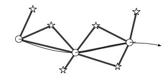
There exists a family of off-line SLAM algorithms which treat the SLAM problems as optimization problem. These techniques exploit a similar independence as discussed in the previous chapter. By retaining all past poses, the set of constraints between different variables in the SLAM posterior can be represented by a set of sparse links. Relaxing those links using conventional optimization techniques then leads to a most likely map and a most likely robot path; assuming known correspondence. Possibly the earliest work on this paradigm is by Lu and Milios [53], which was first implemented by Gutmann [38]. Golfarelli et al. [33] established the relation of SLAM problems and spring-mass models, and Duckett et al. [24] provided a first efficient technique for solving such problems; see also subsequent work in $[48,58]$. The relation between covariances and the information matrix is discussed in [29] and [15]. Folkesson and Christensen introduced a term “Graphical SLAM” into the literature [28], for a related graphical relaxation method. A state-ofthe-art discussion of graphical optimization techniques can be found in [87]. The optimization-based graphical methods are usually offline, and as such are related to the Structure From Motion literature $[43,91]$.

robotics代写|SLAM定位算法代写Simultaneous Localization and Mapping|Robust Data Association

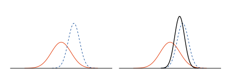
In real SLAM applications, the data associations $n^{t}$ are rarely observable. However, if the uncertainty in landmark positions is low relative to the average distance between landmarks, simple heuristics for determining the correct data association can be quite effective. In particular, the most common approach to data association in SLAM is to assign each observation using a maximum likelihood rule. In other words, each observation is assigned to the landmark most likely to have generated it. If the maximum probability is below some fixed threshold, the observation is considered for addition as a new landmark.
In the case of the EKF, the probability of the observation can be written as a function of the difference between the observation $z_{t}$ and the expected observation $\hat{z}{n{t}}$. This difference is known as the “innovation.”
$$
\begin{aligned}
\hat{n}{t} &=\underset{n{t}}{\operatorname{argmax}} p\left(z_{t} \mid n_{t}, s^{t}, z^{t-1}, u^{t}, \hat{n}^{t-1}\right) \
&=\underset{n_{t}}{\operatorname{argmax}} \frac{1}{\sqrt{\left|2 \pi Z_{t}\right|}} \exp \left{-\frac{1}{2}\left(z_{t}-\hat{z}{n{t}}\right)^{T} Z_{t}^{-1}\left(z_{t}-\hat{z}{n{t}}\right)\right}
\end{aligned}
$$
This data association heuristic is often reformulated in terms of negative $\log$ likelihood, as follows:
$$
\hat{n}{t}=\underset{n{t}}{\operatorname{argmin}} \ln \left|Z_{t}\right|+\left(z_{t}-\hat{z}{n{t}}\right)^{T} Z_{t}^{-1}\left(z_{t}-\hat{z}{n{t}}\right)
$$
The second term of this equation is known as Mahalanobis distance [80], a distance metric normalized by the covariances of the observation and the landmark estimate. For this reason, data association using this metric is often referred to as “nearest neighbor” data association [3], or nearest neighbor gating.

Maximum likelihood data association generally works well when the correct data association is significantly more probable than the incorrect associations. However, if the uncertainty in the landmark positions is high, more than one data association will receive high probability. If a wrong data association is picked, this decision can have a catastrophic result on the accuracy of the resulting map. This kind of data association ambiguity can be induced easily if the robot’s sensors are very noisy.

One approach to this problem is to only incorporate observations that lead to unambiguous data associations (i.e. if only one data association falls within the nearest neighbor threshold). However, if the SLAM environment is noisy, a large percentage of the observations will go unprocessed. Moreover, failing to incorporate observations will lead to overestimated landmark covariances, which makes future data associations even more ambiguous.

A number of more sophisticated approaches to data association have been developed in order to deal with ambiguity in noisy environments.

Complexity
robotics代写|SLAM定位算法代写Simultaneous Localization and Mapping|Scaling SLAM Algorithms

SLAM定位算法代写

robotics代写|SLAM定位算法代写Simultaneous Localization and Mapping|Covariance Intersection

将相关变量视为独立的 SLAM 算法必然会低估它们的协方差。低估协方差会导致分歧并使数据关联变得极其困难。Ulmann 和 Juiler 提出了一种替代方法来维持完整的联合协方差矩阵,称为协方差交点 [45]。Covariance Intersection 保守地更新地标位置方差,以允许观察值和地标之间所有可能的相关性。由于不再需要维护地标之间的相关性,因此生成的 SLAM 算法需要线性时间和内存。不幸的是,地标估计往往非常保守,导致收敛速度极慢和数据关联高度模糊。

robotics代写|SLAM定位算法代写Simultaneous Localization and Mapping|Graphical Optimization Methods

存在一系列将 SLAM 问题视为优化问题的离线 SLAM 算法。这些技术利用了与前一章中讨论的类似的独立性。通过保留所有过去的姿势,SLAM 后验中不同变量之间的约束集可以由一组稀疏链接表示。使用传统的优化技术放松这些链接然后导致最可能的地图和最可能的机器人路径;假设已知对应关系。这种范式的最早工作可能是 Lu 和 Milios [53],它首先由 Gutmann [38] 实现。Golfarelli 等人。[33] 建立了 SLAM 问题和弹簧质量模型的关系,以及 Duckett 等人。[24] 提供了解决此类问题的第一个有效技术;另见后续工作[48,58]. 协方差和信息矩阵之间的关系在[29]和[15]中讨论。Folkesson 和 Christensen 在文献 [28] 中引入了一个术语“图形 SLAM”,用于相关的图形松弛方法。在 [87] 中可以找到关于图形优化技术的最新讨论。基于优化的图形方法通常是离线的,因此与 Structure From Motion 文献有关[43,91].

robotics代写|SLAM定位算法代写Simultaneous Localization and Mapping|Robust Data Association

在真实的 SLAM 应用中,数据关联n吨很少被观察到。但是,如果地标位置的不确定性相对于地标之间的平均距离较低,则用于确定正确数据关联的简单启发式方法可能非常有效。特别是,SLAM 中最常见的数据关联方法是使用最大似然规则分配每个观察值。换句话说,每个观察都被分配给最有可能产生它的地标。如果最大概率低于某个固定阈值,则将观察结果视为添加新地标。
在 EKF 的情况下,观察的概率可以写成观察之间的差异的函数和吨和预期的观察和^n吨. 这种差异被称为“创新”。
\begin{aligned} \hat{n}{t} &=\underset{n{t}}{\operatorname{argmax}} p\left(z_{t} \mid n_{t}, s^{t} , z^{t-1}, u^{t}, \hat{n}^{t-1}\right) \ &=\underset{n_{t}}{\operatorname{argmax}} \frac{ 1}{\sqrt{\left|2 \pi Z_{t}\right|}} \exp \left{-\frac{1}{2}\left(z_{t}-\hat{z}{n {t}}\right)^{T} Z_{t}^{-1}\left(z_{t}-\hat{z}{n{t}}\right)\right} \end{aligned}\begin{aligned} \hat{n}{t} &=\underset{n{t}}{\operatorname{argmax}} p\left(z_{t} \mid n_{t}, s^{t} , z^{t-1}, u^{t}, \hat{n}^{t-1}\right) \ &=\underset{n_{t}}{\operatorname{argmax}} \frac{ 1}{\sqrt{\left|2 \pi Z_{t}\right|}} \exp \left{-\frac{1}{2}\left(z_{t}-\hat{z}{n {t}}\right)^{T} Z_{t}^{-1}\left(z_{t}-\hat{z}{n{t}}\right)\right} \end{aligned}
这种数据关联启发式通常被重新表述为负日志可能性,如下:
n^吨=精氨酸n吨ln⁡|从吨|+(和吨−和^n吨)吨从吨−1(和吨−和^n吨)
该等式的第二项称为马氏距离 [80],它是由观测的协方差和界标估计值归一化的距离度量。出于这个原因,使用此度量的数据关联通常被称为“最近邻”数据关联 [3],或最近邻门控。

当正确的数据关联比不正确的关联更有可能时,最大似然数据关联通常工作得很好。但是,如果地标位置的不确定性很高,则多个数据关联将获得很高的概率。如果选择了错误的数据关联,此决定可能会对结果地图的准确性产生灾难性的影响。如果机器人的传感器噪声很大,则很容易引发这种数据关联模糊。

解决此问题的一种方法是仅合并导致明确数据关联的观察结果(即,如果只有一个数据关联落在最近邻阈值内)。但是,如果 SLAM 环境嘈杂,则很大一部分观察结果将未经处理。此外,未能合并观察将导致高估地标协方差,这使得未来的数据关联更加模糊。

为了处理嘈杂环境中的歧义,已经开发了许多更复杂的数据关联方法。

robotics代写|SLAM定位算法代写Simultaneous Localization and Mapping 请认准statistics-lab™

统计代写请认准statistics-lab™. statistics-lab™为您的留学生涯保驾护航。

金融工程代写

金融工程是使用数学技术来解决金融问题。金融工程使用计算机科学、统计学、经济学和应用数学领域的工具和知识来解决当前的金融问题,以及设计新的和创新的金融产品。

非参数统计代写

非参数统计指的是一种统计方法,其中不假设数据来自于由少数参数决定的规定模型;这种模型的例子包括正态分布模型和线性回归模型。

广义线性模型代考

广义线性模型(GLM)归属统计学领域,是一种应用灵活的线性回归模型。该模型允许因变量的偏差分布有除了正态分布之外的其它分布。

术语 广义线性模型(GLM)通常是指给定连续和/或分类预测因素的连续响应变量的常规线性回归模型。它包括多元线性回归,以及方差分析和方差分析(仅含固定效应)。

有限元方法代写

有限元方法(FEM)是一种流行的方法,用于数值解决工程和数学建模中出现的微分方程。典型的问题领域包括结构分析、传热、流体流动、质量运输和电磁势等传统领域。

有限元是一种通用的数值方法,用于解决两个或三个空间变量的偏微分方程(即一些边界值问题)。为了解决一个问题,有限元将一个大系统细分为更小、更简单的部分,称为有限元。这是通过在空间维度上的特定空间离散化来实现的,它是通过构建对象的网格来实现的:用于求解的数值域,它有有限数量的点。边界值问题的有限元方法表述最终导致一个代数方程组。该方法在域上对未知函数进行逼近。[1] 然后将模拟这些有限元的简单方程组合成一个更大的方程系统,以模拟整个问题。然后,有限元通过变化微积分使相关的误差函数最小化来逼近一个解决方案。

tatistics-lab作为专业的留学生服务机构,多年来已为美国、英国、加拿大、澳洲等留学热门地的学生提供专业的学术服务,包括但不限于Essay代写,Assignment代写,Dissertation代写,Report代写,小组作业代写,Proposal代写,Paper代写,Presentation代写,计算机作业代写,论文修改和润色,网课代做,exam代考等等。写作范围涵盖高中,本科,研究生等海外留学全阶段,辐射金融,经济学,会计学,审计学,管理学等全球99%专业科目。写作团队既有专业英语母语作者,也有海外名校硕博留学生,每位写作老师都拥有过硬的语言能力,专业的学科背景和学术写作经验。我们承诺100%原创,100%专业,100%准时,100%满意。

随机分析代写


随机微积分是数学的一个分支,对随机过程进行操作。它允许为随机过程的积分定义一个关于随机过程的一致的积分理论。这个领域是由日本数学家伊藤清在第二次世界大战期间创建并开始的。

时间序列分析代写

随机过程,是依赖于参数的一组随机变量的全体,参数通常是时间。 随机变量是随机现象的数量表现,其时间序列是一组按照时间发生先后顺序进行排列的数据点序列。通常一组时间序列的时间间隔为一恒定值(如1秒,5分钟,12小时,7天,1年),因此时间序列可以作为离散时间数据进行分析处理。研究时间序列数据的意义在于现实中,往往需要研究某个事物其随时间发展变化的规律。这就需要通过研究该事物过去发展的历史记录,以得到其自身发展的规律。

回归分析代写

多元回归分析渐进(Multiple Regression Analysis Asymptotics)属于计量经济学领域,主要是一种数学上的统计分析方法,可以分析复杂情况下各影响因素的数学关系,在自然科学、社会和经济学等多个领域内应用广泛。

MATLAB代写

MATLAB 是一种用于技术计算的高性能语言。它将计算、可视化和编程集成在一个易于使用的环境中,其中问题和解决方案以熟悉的数学符号表示。典型用途包括:数学和计算算法开发建模、仿真和原型制作数据分析、探索和可视化科学和工程图形应用程序开发,包括图形用户界面构建MATLAB 是一个交互式系统,其基本数据元素是一个不需要维度的数组。这使您可以解决许多技术计算问题,尤其是那些具有矩阵和向量公式的问题,而只需用 C 或 Fortran 等标量非交互式语言编写程序所需的时间的一小部分。MATLAB 名称代表矩阵实验室。MATLAB 最初的编写目的是提供对由 LINPACK 和 EISPACK 项目开发的矩阵软件的轻松访问,这两个项目共同代表了矩阵计算软件的最新技术。MATLAB 经过多年的发展,得到了许多用户的投入。在大学环境中,它是数学、工程和科学入门和高级课程的标准教学工具。在工业领域,MATLAB 是高效研究、开发和分析的首选工具。MATLAB 具有一系列称为工具箱的特定于应用程序的解决方案。对于大多数 MATLAB 用户来说非常重要,工具箱允许您学习应用专业技术。工具箱是 MATLAB 函数(M 文件)的综合集合,可扩展 MATLAB 环境以解决特定类别的问题。可用工具箱的领域包括信号处理、控制系统、神经网络、模糊逻辑、小波、仿真等。

R语言代写问卷设计与分析代写
PYTHON代写回归分析与线性模型代写
MATLAB代写方差分析与试验设计代写
STATA代写机器学习/统计学习代写
SPSS代写计量经济学代写
EVIEWS代写时间序列分析代写
EXCEL代写深度学习代写
SQL代写各种数据建模与可视化代写

robotics代写|SLAM定位算法代写Simultaneous Localization and Mapping|Extended Kalman Filtering

如果你也在 怎样代写SLAM定位算法这个学科遇到相关的难题,请随时右上角联系我们的24/7代写客服。

同步定位和测绘(SLAM)是构建或更新一个未知环境的地图,同时跟踪一个代理在其中的位置的计算问题。虽然这最初似乎是一个鸡生蛋蛋生鸡的问题,但有几种已知的算法可以解决这个问题,至少是近似解决,在某些环境下是可行的。流行的近似解决方法包括粒子过滤器、扩展卡尔曼过滤器、协方差交叉和GraphSLAM。SLAM算法是基于计算几何和计算机视觉的概念,并被用于机器人导航、机器人测绘和虚拟现实或增强现实的里程测量。

statistics-lab™ 为您的留学生涯保驾护航 在代写SLAM定位算法方面已经树立了自己的口碑, 保证靠谱, 高质且原创的统计Statistics代写服务。我们的专家在代写SLAM定位算法代写方面经验极为丰富,各种代写SLAM定位算法相关的作业也就用不着说。

我们提供的SLAM定位算法及其相关学科的代写,服务范围广, 其中包括但不限于:

  • Statistical Inference 统计推断
  • Statistical Computing 统计计算
  • Advanced Probability Theory 高等概率论
  • Advanced Mathematical Statistics 高等数理统计学
  • (Generalized) Linear Models 广义线性模型
  • Statistical Machine Learning 统计机器学习
  • Longitudinal Data Analysis 纵向数据分析
  • Foundations of Data Science 数据科学基础
robotics代写|SLAM定位算法代写Simultaneous Localization and Mapping|Extended Kalman Filtering

robotics代写|SLAM定位算法代写Simultaneous Localization and Mapping|Extended Kalman Filtering

In general, the integral in the recursive update equation (2.15) cannot be computed in closed form. However, approximate SLAM algorithms have been developed by restricting the form of the SLAM posterior, the motion model, and the measurement model. Many of the original SLAM algorithms originate from a seminal paper by Smith and Cheesman [82], which proposed the use of the Extended Kalman Filter (EKF) to estimate the SLAM posterior.

The EKF represents the SLAM posterior as a high-dimensional, multivariate Gaussian parameterized by a mean $\mu_{t}$ and a covariance matrix $\Sigma_{t}$. The mean describes the most likely state of the robot and landmarks, and the covariance matrix encodes the pairwise correlations between all pairs of state variables.
$$
\begin{aligned}
p\left(s_{t}, \Theta \mid u^{t}, z^{t}, n^{t}\right) &=\mathcal{N}\left(x_{t} ; \mu_{t}, \Sigma_{t}\right) \
x_{t} &=\left{s_{t}, \theta_{1}, \ldots, \theta_{N}\right}
\end{aligned}
$$

For robots that move in a plane, the mean vector $\mu_{t}$ is of dimension $2 N+$ 3, where $N$ is the number of landmarks. Three dimensions are required to represent the pose of the robot, and two dimensions are required to specify the position of each landmark. Likewise, the covariance matrix is of size $2 N+3$ by $2 N+3$. Thus, the number of parameters needed to describe the EKF posterior is quadratic in the number of landmarks in the map.

Figure $2.3$ shows a simple example of a Kalman Filter estimating the position of a single landmark in one dimension. Figure $2.3$ (a) shows the current belief in the landmark position (the solid distribution) and a new, noisy observation of the landmark (the dashed distribution). The Kalman Filter describes the optimal procedure for combining Gaussian beliefs in linear systems. In this case, the new posterior after incorporating the dashed observation is shown as a thick line in Figure $2.3(\mathrm{~b})$.

The basic Kalman Filter algorithm is the optimal estimator for a linear system with Gaussian noise [3]. As its name suggests, the EKF is simply an extension of the basic Kalman Filter algorithm to non-linear systems. The EKF does this by replacing the motion and measurement models with nonlinear models that are “linearized” around the most-likely state of the system. In general, this approximation is good if the true models are approximately linear and if the discrete time step of the filter is small.

The motion model will be written as the non-linear function $h\left(x_{t-1}, u_{t}\right)$ with linearized noise covariance $P_{t}$. Similarly, the measurement model will be written as the non-linear function $g\left(x_{t}, n_{t}\right)$ with linearized noise covariance

$R_{t}$. The EKF update equations can be written as follows:
$$
\begin{aligned}
\mu_{t}^{-} &=h\left(\mu_{t-1}, u_{t}\right) \
\Sigma_{t}^{-} &=\Sigma_{t-1}+P_{t} \
G_{x} &=\left.\nabla_{x_{t}} g\left(x_{t}, n_{t}\right)\right|{x{t}=\mu_{t}^{-} ; n_{t}=n_{t}} \
Z_{t} &=G_{x} \Sigma_{t}^{-} G_{x}^{T}+R_{t} \quad \hat{z}{n{t}}=g\left(\mu_{t}^{-}, n_{t}\right) \
K_{t} &=\Sigma_{t}^{-} G_{x}^{T} Z_{t}^{-1} \
\mu_{t} &=\mu_{t}^{-}+K_{t}\left(z_{t}-\hat{z}{n{t}}\right) \
\Sigma_{t} &=\left(I-K_{t} G_{t}\right) \Sigma_{t}^{-}
\end{aligned}
$$
For a complete derivation of the Kalman Filter, see $[46,31,87]$, and for a gentle introduction to the use of the Kalman Filter and the EKF, see $[95]$. It is important to note that if the SLAM problem is linear and Gaussian, then the Kalman Filter is both guaranteed to converge [69] and provably optimal [3]. Real-world SLAM problems are rarely linear, yet the EKF still tends to produce very good results in general. For this reason, the EKF is often held up as the “gold standard” of comparison for online SLAM algorithms.
The EKF has two substantial disadvantages when applied to the SLAM problem: quadratic complexity and sensitivity to failures in data association. The number of mathematical operations required to incorporate a control and an observation into the filter is dominated by the final EKF update equation (2.26). In the planar case, both $K_{t}$ and $G_{t}^{T}$ are of dimension $2 N+3$ by the dimensionality of the observation (typically two). Thus, the inner product in the calculation of $\Sigma_{t}$ requires a number of calculations quadratic with the number of landmarks $N$.

The second problem with the EKF applies in situations in which the data associations $n_{t}$ are unknown. The EKF maintains a single data association hypothesis per observation, typically chosen using a maximum likelihood heuristic. If the probability of an observation coming from any of the current landmarks is too low, the possibility of a new landmark is considered. If the data association chosen by this heuristic is incorrect, the effect of incorporating this observation into the EKF can never be removed. If many observations are incorporated into the EKF with wrong data associations, the EKF will diverge. This is a well known failure mode of the EKF [18]. The following sections will describe alternative approaches to SLAM that address the issues of efficient scaling and robust data association.

robotics代写|SLAM定位算法代写Simultaneous Localization and Mapping|Submap Methods

While the Kalman Filter is the optimal solution to the linear-Gaussian SLAM problem, it is computationally infeasible for large maps. As a result, a great

deal of SLAM research has concentrated on developing SLAM algorithms that approximate the performance of the EKF, but scale to much larger environments. The computational complexity of the EKF stems from the fact that covariance matrix $\Sigma_{t}$ represents every pairwise correlation between the state variables. Incorporating an observation of a single landmark will necessarily have an affect on every other state variable.

Typically, the observation of a single landmark will have a weak effect on the positions of distant landmarks. For this reason, many researchers have developed EKF-based SLAM algorithms that decompose the global map into smaller submaps. One set of approaches exploits the fact that the robot may linger for some period of time in a small section of the global map. Postponement $[10,47]$, and the Compressed Extended Kalman Filter (CEKF) [36], are both techniques that delay the incorporation of local information into the global map while the robot stays inside a single submap. These techniques are still optimal, in that they generate the same results as the full EKF. However, the computation required by the two algorithms is reduced by a constant factor because the full map updates are performed less frequently.

Breaking the global map into submaps can also lead to a more sparse description of the correlations between map elements. Increased sparsity can be exploited to compute more efficient sensor updates. Network Coupled Feature Maps [1], ATLAS [5], the Local Mapping Algorithm [7], and the Decoupled Stochastic Mapping [49] frameworks all consider relationships between a sparse network of submaps. When the robot moves out of one submap, it either creates a new submap or relocates itself in a previously defined submap. Each approach reduces the computational requirement of incorporating an observation to constant time, given known data association. However, these computational gains come at the cost of slowing down the overall rate of convergence. Each map has far fewer features than the overall map would have, and the effects of observations on distant landmarks may have to percolate through multiple correlation links.

Guivant and Nebot presented a similar method called Suboptimal SLAM $[36]$, in which the local maps are all computed with respect to a small number of base landmarks. Since the different constellations of landmarks are kept in different coordinate frames, they can be decorrelated more easily than if every landmark were in a single coordinate frame. The resulting algorithm produces an estimate that is an approximation to the true EKF estimate, however it requires linear time and memory.

robotics代写|SLAM定位算法代写Simultaneous Localization and Mapping|Sparse Extended Information Filters

Another filter approach to decomposing the SLAM problem is to represent maps using potential functions between nearby landmarks, similar to Markov Random Fields [6]. One such approach is the Sparse Extended Information Filter (SEIF) proposed in [90]. SEIFs implement an alternate parameterization of the Kalman Filter, called the Information Filter. Instead of updating a covariance matrix $\Sigma$, SEIFs update $\Sigma^{-1}$, the precision matrix. This parameterization is useful because the precision matrix is sparse if correlations are maintained only between nearby landmarks. Under appropriate approximations, this technique has been shown to provide efficient updates (given known data association) with a linear memory requirement.

The Thin Junction Tree Filter (TJTF) of Paskin [73] is a SLAM algorithm based on the same principle as the SEIF. Namely, maintaining a sparse network of probabilistic constraints between state variables enables efficient inference. The TJTF represents the SLAM posterior using a graphical model called a junction tree. The size of the junction tree grows as new landmarks are added to the map, but it can be “thinned” using an operation called variable contraction. The thinning operation can be viewed as a method for making the precision matrix of a SEIF sparse, however global maps can be extracted from TJTFs without any matrix inversion. TJTFs require linear computation in general, which can be reduced to constant time with further approximation.

robotics代写|SLAM定位算法代写Simultaneous Localization and Mapping|Extended Kalman Filtering

SLAM定位算法代写

robotics代写|SLAM定位算法代写Simultaneous Localization and Mapping|Extended Kalman Filtering

一般来说,递归更新方程(2.15)中的积​​分不能以封闭形式计算。然而,通过限制 SLAM 后验、运动模型和测量模型的形式,已经开发了近似 SLAM 算法。许多原始的 SLAM 算法源自 Smith 和 Cheesman [82] 的一篇开创性论文,该论文提出使用扩展卡尔曼滤波器 (EKF) 来估计 SLAM 后验。

EKF 将 SLAM 后验表示为由均值参数化的高维、多元高斯μ吨和协方差矩阵Σ吨. 均值描述了机器人和地标最可能的状态,协方差矩阵编码了所有状态变量对之间的成对相关性。
\begin{对齐} p\left(s_{t}, \Theta \mid u^{t}, z^{t}, n^{t}\right) &=\mathcal{N}\left(x_{ t} ; \mu_{t}, \Sigma_{t}\right) \ x_{t} &=\left{s_{t}, \theta_{1}, \ldots, \theta_{N}\right} \结束{对齐}\begin{对齐} p\left(s_{t}, \Theta \mid u^{t}, z^{t}, n^{t}\right) &=\mathcal{N}\left(x_{ t} ; \mu_{t}, \Sigma_{t}\right) \ x_{t} &=\left{s_{t}, \theta_{1}, \ldots, \theta_{N}\right} \结束{对齐}

对于在平面上移动的机器人,平均向量μ吨有维度2ñ+3、哪里ñ是地标的数量。需要三个维度来表示机器人的位姿,并且需要两个维度来指定每个地标的位置。同样,协方差矩阵的大小2ñ+3经过2ñ+3. 因此,描述 EKF 后验所需的参数数量是地图中地标数量的二次方。

数字2.3显示了一个简单的卡尔曼滤波器示例,它估计单个地标在一维中的位置。数字2.3(a) 显示了对地标位置的当前信念(实线分布)和对地标的新的嘈杂观察(虚线分布)。卡尔曼滤波器描述了在线性系统中组合高斯信念的最佳过程。在这种情况下,合并虚线观察后的新后验在图中显示为粗线2.3( b).

基本的卡尔曼滤波器算法是具有高斯噪声的线性系统的最佳估计器 [3]。顾名思义,EKF 只是基本卡尔曼滤波器算法对非线性系统的扩展。EKF 通过用围绕系统最可能状态“线性化”的非线性模型替换运动和测量模型来做到这一点。一般来说,如果真实模型近似线性并且滤波器的离散时间步长很小,则这种近似是好的。

运动模型将被写成非线性函数H(X吨−1,在吨)具有线性化噪声协方差磷吨. 类似地,测量模型将被写为非线性函数G(X吨,n吨)具有线性化噪声协方差

R吨. EKF 更新方程可以写成如下:
$$
\begin{aligned}
\mu_{t}^{-} &=h\left(\mu_{t-1}, u_{t}\right) \
\Sigma_ {t}^{-} &=\Sigma_{t-1}+P_{t} \
G_{x} &=\left.\nabla_{x_{t}} g\left(x_{t}, n_{ t}\右)\右| {x {t}=\mu_{t}^{-} ; n_{t}=n_{t}} \
Z_{t} &=G_{x} \Sigma_{t}^{-} G_{x}^{T}+R_{t} \quad \hat{z} {n {t}}=g\left(\mu_{t}^{-}, n_{t}\right) \
K_{t} &=\Sigma_{t}^{-} G_{x}^{ T} Z_{t}^{-1} \
\mu_{t} &=\mu_{t}^{-}+K_{t}\left(z_{t}-\hat{z} {n {t }}\right) \
\Sigma_{t} &=\left(I-K_{t} G_{t}\right) \Sigma_{t}^{-} \
end{aligned}
$$
卡尔曼滤波器,见[46,31,87],关于卡尔曼滤波器和 EKF 的使用的简要介绍,请参阅[95]. 重要的是要注意,如果 SLAM 问题是线性和高斯问题,那么卡尔曼滤波器既可以保证收敛 [69] 又可以证明是最优的 [3]。现实世界的 SLAM 问题很少是线性的,但是 EKF 通常仍然倾向于产生非常好的结果。出于这个原因,EKF 通常被认为是在线 SLAM 算法比较的“黄金标准”。
当应用于 SLAM 问题时,EKF 有两个实质性的缺点:二次复杂性和对数据关联失败的敏感性。将控制和观察合并到滤波器中所需的数学运算的数量由最终的 EKF 更新方程 (2.26) 决定。在平面情况下,两者ķ吨和G吨吨有维度2ñ+3通过观察的维度(通常是两个)。因此,计算中的内积Σ吨需要多次计算与地标的数量成二次方ñ.

EKF 的第二个问题适用于数据关联的情况n吨是未知的。EKF 维护每个观察的单个数据关联假设,通常使用最大似然启发式选择。如果观测来自任何当前地标的概率太低,则考虑新地标的可能性。如果此启发式选择的数据关联不正确,则永远无法消除将此观察结果纳入 EKF 的效果。如果将许多观察结果与错误的数据关联合并到 EKF 中,则 EKF 将发散。这是 EKF [18] 众所周知的故障模式。以下部分将描述 SLAM 的替代方法,以解决有效扩展和稳健数据关联的问题。

robotics代写|SLAM定位算法代写Simultaneous Localization and Mapping|Submap Methods

虽然卡尔曼滤波器是线性高斯 SLAM 问题的最佳解决方案,但它对于大型地图在计算上是不可行的。结果,一个伟大的

SLAM 研究的重点是开发 SLAM 算法,该算法接近 EKF 的性能,但可以扩展到更大的环境。EKF 的计算复杂性源于协方差矩阵Σ吨表示状态变量之间的每个成对相关性。结合对单个地标的观察必然会对所有其他状态变量产生影响。

通常,单个地标的观察将对远处地标的位置产生微弱的影响。出于这个原因,许多研究人员开发了基于 EKF 的 SLAM 算法,将全局地图分解为更小的子图。一组方法利用了机器人可能会在全球地图的一小部分逗留一段时间的事实。延期[10,47]和 Compressed Extended Kalman Filter (CEKF) [36] 都是在机器人停留在单个子图内时延迟将局部信息合并到全局地图中的技术。这些技术仍然是最佳的,因为它们产生的结果与完整的 EKF 相同。然而,这两种算法所需的计算量减少了一个常数因子,因为全图更新的执行频率较低。

将全局地图分解为子地图也可能导致对地图元素之间相关性的描述更加稀疏。可以利用增加的稀疏性来计算更有效的传感器更新。网络耦合特征图 [1]、ATLAS [5]、局部映射算法 [7] 和解耦随机映射 [49] 框架都考虑了子图的稀疏网络之间的关系。当机器人移出一个子图时,它要么创建一个新的子图,要么将自己重新定位到先前定义的子图中。给定已知的数据关联,每种方法都减少了将观察合并到恒定时间的计算要求。然而,这些计算增益是以降低整体收敛速度为代价的。每张地图的特征远少于整个地图的特征,

Guivant 和 Nebot 提出了一种类似的方法,称为次优 SLAM[36],其中局部地图都是针对少量基本地标计算的。由于地标的不同星座保存在不同的坐标系中,因此与每个地标都在单个坐标系中相比,它们可以更容易地去相关。结果算法产生的估计值是真实 EKF 估计值的近似值,但是它需要线性时间和内存。

robotics代写|SLAM定位算法代写Simultaneous Localization and Mapping|Sparse Extended Information Filters

分解 SLAM 问题的另一种过滤方法是使用附近地标之间的势函数来表示地图,类似于马尔可夫随机场 [6]。一种这样的方法是[90]中提出的稀疏扩展信息过滤器(SEIF)。SEIF 实现了卡尔曼滤波器的替代参数化,称为信息滤波器。而不是更新协方差矩阵Σ, SEIF 更新Σ−1,精度矩阵。此参数化很有用,因为如果仅在附近地标之间保持相关性,则精度矩阵是稀疏的。在适当的近似下,该技术已被证明可以提供具有线性内存需求的有效更新(给定已知数据关联)。

Paskin [73] 的 Thin Junction Tree Filter (TJTF) 是一种基于与 SEIF 相同原理的 SLAM 算法。也就是说,在状态变量之间维护一个稀疏的概率约束网络可以实现有效的推理。TJTF 使用称为连接树的图形模型表示 SLAM 后验。随着新地标添加到地图中,连接树的大小会增长,但可以使用称为变量收缩的操作“细化”它。细化操作可以看作是一种使 SEIF 的精度矩阵稀疏的方法,但是可以从 TJTF 中提取全局映射而无需任何矩阵求逆。TJTF 通常需要线性计算,可以通过进一步近似将其简化为恒定时间。

robotics代写|SLAM定位算法代写Simultaneous Localization and Mapping 请认准statistics-lab™

统计代写请认准statistics-lab™. statistics-lab™为您的留学生涯保驾护航。

金融工程代写

金融工程是使用数学技术来解决金融问题。金融工程使用计算机科学、统计学、经济学和应用数学领域的工具和知识来解决当前的金融问题,以及设计新的和创新的金融产品。

非参数统计代写

非参数统计指的是一种统计方法,其中不假设数据来自于由少数参数决定的规定模型;这种模型的例子包括正态分布模型和线性回归模型。

广义线性模型代考

广义线性模型(GLM)归属统计学领域,是一种应用灵活的线性回归模型。该模型允许因变量的偏差分布有除了正态分布之外的其它分布。

术语 广义线性模型(GLM)通常是指给定连续和/或分类预测因素的连续响应变量的常规线性回归模型。它包括多元线性回归,以及方差分析和方差分析(仅含固定效应)。

有限元方法代写

有限元方法(FEM)是一种流行的方法,用于数值解决工程和数学建模中出现的微分方程。典型的问题领域包括结构分析、传热、流体流动、质量运输和电磁势等传统领域。

有限元是一种通用的数值方法,用于解决两个或三个空间变量的偏微分方程(即一些边界值问题)。为了解决一个问题,有限元将一个大系统细分为更小、更简单的部分,称为有限元。这是通过在空间维度上的特定空间离散化来实现的,它是通过构建对象的网格来实现的:用于求解的数值域,它有有限数量的点。边界值问题的有限元方法表述最终导致一个代数方程组。该方法在域上对未知函数进行逼近。[1] 然后将模拟这些有限元的简单方程组合成一个更大的方程系统,以模拟整个问题。然后,有限元通过变化微积分使相关的误差函数最小化来逼近一个解决方案。

tatistics-lab作为专业的留学生服务机构,多年来已为美国、英国、加拿大、澳洲等留学热门地的学生提供专业的学术服务,包括但不限于Essay代写,Assignment代写,Dissertation代写,Report代写,小组作业代写,Proposal代写,Paper代写,Presentation代写,计算机作业代写,论文修改和润色,网课代做,exam代考等等。写作范围涵盖高中,本科,研究生等海外留学全阶段,辐射金融,经济学,会计学,审计学,管理学等全球99%专业科目。写作团队既有专业英语母语作者,也有海外名校硕博留学生,每位写作老师都拥有过硬的语言能力,专业的学科背景和学术写作经验。我们承诺100%原创,100%专业,100%准时,100%满意。

随机分析代写


随机微积分是数学的一个分支,对随机过程进行操作。它允许为随机过程的积分定义一个关于随机过程的一致的积分理论。这个领域是由日本数学家伊藤清在第二次世界大战期间创建并开始的。

时间序列分析代写

随机过程,是依赖于参数的一组随机变量的全体,参数通常是时间。 随机变量是随机现象的数量表现,其时间序列是一组按照时间发生先后顺序进行排列的数据点序列。通常一组时间序列的时间间隔为一恒定值(如1秒,5分钟,12小时,7天,1年),因此时间序列可以作为离散时间数据进行分析处理。研究时间序列数据的意义在于现实中,往往需要研究某个事物其随时间发展变化的规律。这就需要通过研究该事物过去发展的历史记录,以得到其自身发展的规律。

回归分析代写

多元回归分析渐进(Multiple Regression Analysis Asymptotics)属于计量经济学领域,主要是一种数学上的统计分析方法,可以分析复杂情况下各影响因素的数学关系,在自然科学、社会和经济学等多个领域内应用广泛。

MATLAB代写

MATLAB 是一种用于技术计算的高性能语言。它将计算、可视化和编程集成在一个易于使用的环境中,其中问题和解决方案以熟悉的数学符号表示。典型用途包括:数学和计算算法开发建模、仿真和原型制作数据分析、探索和可视化科学和工程图形应用程序开发,包括图形用户界面构建MATLAB 是一个交互式系统,其基本数据元素是一个不需要维度的数组。这使您可以解决许多技术计算问题,尤其是那些具有矩阵和向量公式的问题,而只需用 C 或 Fortran 等标量非交互式语言编写程序所需的时间的一小部分。MATLAB 名称代表矩阵实验室。MATLAB 最初的编写目的是提供对由 LINPACK 和 EISPACK 项目开发的矩阵软件的轻松访问,这两个项目共同代表了矩阵计算软件的最新技术。MATLAB 经过多年的发展,得到了许多用户的投入。在大学环境中,它是数学、工程和科学入门和高级课程的标准教学工具。在工业领域,MATLAB 是高效研究、开发和分析的首选工具。MATLAB 具有一系列称为工具箱的特定于应用程序的解决方案。对于大多数 MATLAB 用户来说非常重要,工具箱允许您学习应用专业技术。工具箱是 MATLAB 函数(M 文件)的综合集合,可扩展 MATLAB 环境以解决特定类别的问题。可用工具箱的领域包括信号处理、控制系统、神经网络、模糊逻辑、小波、仿真等。

R语言代写问卷设计与分析代写
PYTHON代写回归分析与线性模型代写
MATLAB代写方差分析与试验设计代写
STATA代写机器学习/统计学习代写
SPSS代写计量经济学代写
EVIEWS代写时间序列分析代写
EXCEL代写深度学习代写
SQL代写各种数据建模与可视化代写

robotics代写|SLAM定位算法代写Simultaneous Localization and Mapping|The SLAM Problem

如果你也在 怎样代写SLAM定位算法这个学科遇到相关的难题,请随时右上角联系我们的24/7代写客服。

同步定位和测绘(SLAM)是构建或更新一个未知环境的地图,同时跟踪一个代理在其中的位置的计算问题。虽然这最初似乎是一个鸡生蛋蛋生鸡的问题,但有几种已知的算法可以解决这个问题,至少是近似解决,在某些环境下是可行的。流行的近似解决方法包括粒子过滤器、扩展卡尔曼过滤器、协方差交叉和GraphSLAM。SLAM算法是基于计算几何和计算机视觉的概念,并被用于机器人导航、机器人测绘和虚拟现实或增强现实的里程测量。

statistics-lab™ 为您的留学生涯保驾护航 在代写SLAM定位算法方面已经树立了自己的口碑, 保证靠谱, 高质且原创的统计Statistics代写服务。我们的专家在代写SLAM定位算法代写方面经验极为丰富,各种代写SLAM定位算法相关的作业也就用不着说。

我们提供的SLAM定位算法及其相关学科的代写,服务范围广, 其中包括但不限于:

  • Statistical Inference 统计推断
  • Statistical Computing 统计计算
  • Advanced Probability Theory 高等概率论
  • Advanced Mathematical Statistics 高等数理统计学
  • (Generalized) Linear Models 广义线性模型
  • Statistical Machine Learning 统计机器学习
  • Longitudinal Data Analysis 纵向数据分析
  • Foundations of Data Science 数据科学基础
robotics代写|SLAM定位算法代写Simultaneous Localization and Mapping|The SLAM Problem

robotics代写|SLAM定位算法代写Simultaneous Localization and Mapping|SLAM Posterior

The pose of the robot at time $t$ will be denoted $s_{t}$. For a robot operating in a planar environment, this pose consists of the robot’s $x-y$ position in the plane and its heading direction. All experimental results presented in this book were generated in planar environments, however the algorithms apply equally well to three-dimensional worlds. The complete trajectory of the robot, consisting of the robot’s pose at every time step, will be written as $s^{t}$.
$$
s^{t}=\left{s_{1}, s_{2}, \ldots, s_{t}\right}
$$
We shall further assume that the robot’s environment can be modeled as a set of $N$ immobile, point landmarks. Point landmarks are commonly used to represent the locations of features extracted from sensor data, such as geometric features in a laser scan or distinctive visual features in a camera image. The set of $N$ landmark locations will be written $\left{\theta_{1}, \ldots, \theta_{N}\right}$. For notational simplicity, the entire map will be written as $\Theta$.

As the robot moves through the environment, it collects relative information about its own motion. This information can be generated using odometers attached to the wheels of the robot, inertial navigation units, or simply by observing the control commands executed by the robot. Regardless of origin, any measurement of the robot’s motion will be referred to generically as a control. The control at time $t$ will be written $u_{t}$. The set of all controls executed by the robot will be written $u^{t}$.
$$
u^{t}=\left{u_{1}, u_{2}, \ldots, u_{t}\right}
$$
As the robot moves through its environment, it observes nearby landmarks. In the most common formulation of the planar SLAM problem, the robot observes both the range and bearing to nearby obstacles. The observation at time $t$ will be written $z_{t}$. The set of all observations collected by the robot will be written $z^{t}$.
$$
z^{t}=\left{z_{1}, z_{2}, \ldots, z_{t}\right}
$$

It is commonly assumed in the SLAM literature that sensor measurements can be decomposed into information about individual landmarks, such that each landmark observation can be incorporated independently from the other measurements. This is a realistic assumption in virtually all successful SLAM implementations, where landmark features are extracted one-by-one from raw sensor data. Thus, we will assume that each observation provides information about the location of exactly one landmark $\theta_{n}$ relative to the robot’s current pose $s_{t}$. The variable $n$ represents the identity of the landmark being observed. In practice, the identities of landmarks usually can not be observed, as many landmarks may look alike. The identity of the landmark corresponding to the observation $z_{t}$ will be written as $n_{t}$, where $n_{t} \in{1, \ldots, N}$. For example, $n_{8}=3$ means that at time $t=8$ the robot observed the third landmark. Landmark identities are commonly referred to as “data associations” or “correspondences.” The set of all data associations will be written $n^{t}$.
$$
n^{t}=\left{n_{1}, n_{2}, \ldots, n_{t}\right}
$$
Again for simplicity, we will assume that the robot receives exactly one measurement $z_{t}$ and executes exactly one control $u_{t}$ per time step. Multiple observations per time step can be processed sequentially, but this leads to a more cumbersome notation.

Using the notation defined above, the primary goal of SLAM is to recover the best estimate of the robot pose $s_{t}$ and the map $\Theta$, given the set of noisy observations $z^{t}$ and controls $u^{t}$. In probabilistic terms, this is expressed by the following posterior:
$$
p\left(s_{t}, \Theta \mid z^{t}, u^{t}\right)
$$
If the set of data associations $n^{t}$ is also given, the posterior can be rewritten as:
$$
p\left(s_{t}, \Theta \mid z^{t}, u^{t}, n^{t}\right)
$$

robotics代写|SLAM定位算法代写Simultaneous Localization and Mapping|SLAM as a Markov Chain

The SLAM problem can be described best as a probabilistic Markov chain. A graphical depiction of this Markov chain is shown in Figure 2.2. The current pose of the robot $s_{t}$ can be written as a probabilistic function of the pose at the previous time step $s_{t-1}$ and the control $u_{t}$ executed by the robot. This function is referred to as the motion model because it describes how controls drive the motion of the robot. Additionally, the motion model describes how noise in the controls injects uncertainty into the robot’s pose estimate. The motion model is written as:
$$
p\left(s_{t} \mid s_{t-1}, u_{t}\right)
$$
Sensor observations gathered by the robot are also governed by a probabilistic function, commonly referred to as the measurement model. The observation $z_{t}$

is a function of the observed landmark $\theta_{n_{t}}$ and the pose of the robot $s_{t}$. The measurement model describes the physics and the error model of the robot’s sensor. The measurement model is written as:
$$
p\left(z_{t} \mid s_{t}, \Theta, n_{t}\right)
$$
Using the motion model and the measurement model, the SLAM posterior at time $t$ can be computed recursively as function of the posterior at time $t-1$. This recursive update rule, known as the Bayes filter for SLAM, is the basis for the majority of online SLAM algorithms.

robotics代写|SLAM定位算法代写Simultaneous Localization and Mapping|Bayes Filter Derivation

The Bayes Filter can be derived from the SLAM posterior as follows. First, the posterior (2.6) is rewritten using Bayes Rule.
$$
p\left(s_{t}, \Theta \mid z^{t}, u^{t}, n^{t}\right)=\eta p\left(z_{t} \mid s_{t}, \Theta, z^{t-1}, u^{t}, n^{t}\right) p\left(s_{t}, \Theta \mid z^{t-1}, u^{t}, n^{t}\right)
$$
The denominator from Bayes rule is a normalizing constant and is written as $\eta$. Next, we exploit the fact that $z_{t}$ is solely a function of the pose of the robot $s_{t}$, the map $\Theta$, and the latest data association $n_{t}$, previously described as the measurement model. Hence the posterior becomes:
$$
=\eta p\left(z_{t} \mid s_{t}, \Theta, n_{t}\right) p\left(s_{t}, \Theta \mid z^{t-1}, u^{t}, n^{t}\right)
$$
Now we use the Theorem of Total Probability to condition the rightmost term of $(2.10)$ on the pose of the robot at time $t-1$.
$$
=\eta p\left(z_{t} \mid s_{t}, \Theta, n_{t}\right) \int p\left(s_{t}, \Theta \mid s_{t-1}, z^{t-1}, u^{t}, n^{t}\right) p\left(s_{t-1} \mid z^{t-1}, u^{t}, n^{t}\right) d s_{t-1}
$$

The leftmost term inside the integral can be expanded using the definition of conditional probability.
$$
\begin{aligned}
&=\eta p\left(z_{t} \mid s_{t}, \Theta, n_{t}\right) \
&\int p\left(s_{t} \mid \Theta, s_{t-1}, z^{t-1}, u^{t}, n^{t}\right) p\left(\Theta \mid s_{t-1}, z^{t-1}, u^{t}, n^{t}\right) p\left(s_{t-1} \mid z^{t-1}, u^{t}, n^{t}\right) d s_{t-1}
\end{aligned}
$$
The first term inside the integral can now be simplified by noting that $s_{t}$ is only a function of $s_{t-1}$ and $u_{t}$, previously described as the motion model.
$$
\begin{aligned}
&=\eta p\left(z_{t} \mid s_{t}, \Theta, n_{t}\right) \
&\qquad \int p\left(s_{t} \mid s_{t-1}, u_{t}\right) p\left(\Theta \mid s_{t-1}, z^{t-1}, u^{t}, n^{t}\right) p\left(s_{t-1} \mid z^{t-1}, u^{t}, n^{t}\right) d s_{t-1}
\end{aligned}
$$
At this point, the two rightmost terms in the integral can be combined.
$$
=\eta p\left(z_{t} \mid s_{t}, \Theta, n_{t}\right) \int p\left(s_{t} \mid s_{t-1}, u_{t}\right) p\left(s_{t-1}, \Theta \mid z^{t-1}, u^{t}, n^{t}\right) d s_{t-1}
$$
Since the current pose $u_{t}$ and data association $n_{t}$ provide no new information about $s_{t-1}$ or $\Theta$ without the latest observation $z_{t}$, they can be dropped from the rightmost term of the integral. The result is a recursive formula for computing the SLAM posterior at time $t$ given the SLAM posterior at time $t-1$, the motion model $p\left(s_{t} \mid s_{t-1}, u_{t}\right)$, and the measurement model $p\left(z_{t} \mid s_{t}, \Theta, n_{t}\right)$.
$$
\begin{aligned}
&p\left(s_{t}, \Theta \mid z^{t}, u^{t}, n^{t}\right)= \
&\eta p\left(z_{t} \mid s_{t}, \Theta, n_{t}\right) \int p\left(s_{t} \mid s_{t-1}, u_{t}\right) p\left(s_{t-1}, \Theta \mid z^{t-1}, u^{t-1}, n^{t-1}\right) d s_{t-1}
\end{aligned}
$$

robotics代写|SLAM定位算法代写Simultaneous Localization and Mapping|The SLAM Problem

SLAM定位算法代写

robotics代写|SLAM定位算法代写Simultaneous Localization and Mapping|SLAM Posterior

机器人当时的姿势吨将表示s吨. 对于在平面环境中运行的机器人,该位姿由机器人的X−是在平面上的位置及其航向。本书中介绍的所有实验结果都是在平面环境中生成的,但是算法同样适用于三维世界。机器人的完整轨迹,包括机器人在每个时间步的位姿,将被写为s吨.
s^{t}=\left{s_{1}, s_{2}, \ldots, s_{t}\right}s^{t}=\left{s_{1}, s_{2}, \ldots, s_{t}\right}
我们将进一步假设机器人的环境可以建模为一组ñ不动,点地标。点地标通常用于表示从传感器数据中提取的特征的位置,例如激光扫描中的几何特征或相机图像中的独特视觉特征。该组ñ地标位置将被写入\left{\theta_{1}, \ldots, \theta_{N}\right}\left{\theta_{1}, \ldots, \theta_{N}\right}. 为了符号简单,整个地图将被写为θ.

当机器人在环境中移动时,它会收集有关其自身运动的相关信息。这些信息可以使用附在机器人轮子上的里程表、惯性导航单元或简单地通过观察机器人执行的控制命令来生成。无论起源如何,对机器人运动的任何测量都将统称为控制。当时的控制吨会写在吨. 机器人执行的所有控制的集合将被写入在吨.
u^{t}=\left{u_{1}, u_{2}, \ldots, u_{t}\right}u^{t}=\left{u_{1}, u_{2}, \ldots, u_{t}\right}
当机器人在其环境中移动时,它会观察附近的地标。在平面 SLAM 问题的最常见公式中,机器人观察到附近障碍物的范围和方位。当时的观察吨会写和吨. 机器人收集的所有观测值的集合将被写入和吨.
z^{t}=\left{z_{1}, z_{2}, \ldots, z_{t}\right}z^{t}=\left{z_{1}, z_{2}, \ldots, z_{t}\right}

在 SLAM 文献中通常假设传感器测量可以分解为有关单个地标的信息,这样每个地标观察可以独立于其他测量值合并。在几乎所有成功的 SLAM 实现中,这是一个现实的假设,其中地标特征是从原始传感器数据中一一提取的。因此,我们将假设每个观测都提供了关于恰好一个地标位置的信息θn相对于机器人的当前姿势s吨. 变量n表示被观察的地标的身份。在实践中,通常无法观察到地标的身份,因为许多地标可能看起来很相似。与观测对应的地标的身份和吨将被写为n吨, 在哪里n吨∈1,…,ñ. 例如,n8=3意味着当时吨=8机器人观察到了第三个地标。地标身份通常被称为“数据关联”或“通信”。将写入所有数据关联的集合n吨.
n^{t}=\left{n_{1}, n_{2}, \ldots, n_{t}\right}n^{t}=\left{n_{1}, n_{2}, \ldots, n_{t}\right}
再次为简单起见,我们将假设机器人只接收一次测量值和吨并且只执行一个控件在吨每个时间步。每个时间步的多个观测值可以按顺序处理,但这会导致更繁琐的表示法。

使用上面定义的符号,SLAM 的主要目标是恢复机器人姿态的最佳估计s吨和地图θ,给定一组嘈杂的观测值和吨和控制在吨. 在概率方面,这由以下后验表示:
p(s吨,θ∣和吨,在吨)
如果数据关联集n吨同样给出,后验可以重写为:
p(s吨,θ∣和吨,在吨,n吨)

robotics代写|SLAM定位算法代写Simultaneous Localization and Mapping|SLAM as a Markov Chain

SLAM 问题可以最好地描述为概率马尔可夫链。该马尔可夫链的图形描述如图 2.2 所示。机器人当前位姿s吨可以写成前一个时间步的位姿的概率函数s吨−1和控制在吨由机器人执行。这个函数被称为运动模型,因为它描述了控制如何驱动机器人的运动。此外,运动模型描述了控制中的噪声如何将不确定性注入到机器人的姿态估计中。运动模型写为:
p(s吨∣s吨−1,在吨)
机器人收集的传感器观察结果也受概率函数控制,通常称为测量模型。观察和吨

是观察到的地标的函数θn吨和机器人的姿势s吨. 测量模型描述了机器人传感器的物理特性和误差模型。测量模型写为:
p(和吨∣s吨,θ,n吨)
使用运动模型和测量模型,SLAM 后验时间吨可以递归地计算为时间的后验函数吨−1. 这种递归更新规则,称为 SLAM 的贝叶斯过滤器,是大多数在线 SLAM 算法的基础。

robotics代写|SLAM定位算法代写Simultaneous Localization and Mapping|Bayes Filter Derivation

贝叶斯滤波器可以从 SLAM 后验推导出来,如下所示。首先,使用贝叶斯规则重写后验(2.6)。
p(s吨,θ∣和吨,在吨,n吨)=这p(和吨∣s吨,θ,和吨−1,在吨,n吨)p(s吨,θ∣和吨−1,在吨,n吨)
贝叶斯规则的分母是归一化常数,写为这. 接下来,我们利用以下事实和吨仅是机器人姿态的函数s吨, 地图θ,以及最新的数据关联n吨,之前描述为测量模型。因此后验变为:
=这p(和吨∣s吨,θ,n吨)p(s吨,θ∣和吨−1,在吨,n吨)
现在我们使用总概率定理来调节最右边的项(2.10)关于机器人当时的位姿吨−1.
=这p(和吨∣s吨,θ,n吨)∫p(s吨,θ∣s吨−1,和吨−1,在吨,n吨)p(s吨−1∣和吨−1,在吨,n吨)ds吨−1

积分内最左边的项可以使用条件概率的定义进行扩展。
=这p(和吨∣s吨,θ,n吨) ∫p(s吨∣θ,s吨−1,和吨−1,在吨,n吨)p(θ∣s吨−1,和吨−1,在吨,n吨)p(s吨−1∣和吨−1,在吨,n吨)ds吨−1
积分内的第一项现在可以简化为:s吨只是一个函数s吨−1和在吨,之前描述为运动模型。
=这p(和吨∣s吨,θ,n吨) ∫p(s吨∣s吨−1,在吨)p(θ∣s吨−1,和吨−1,在吨,n吨)p(s吨−1∣和吨−1,在吨,n吨)ds吨−1
此时,积分中最右边的两项可以合并。
=这p(和吨∣s吨,θ,n吨)∫p(s吨∣s吨−1,在吨)p(s吨−1,θ∣和吨−1,在吨,n吨)ds吨−1
由于当前姿势在吨和数据关联n吨不提供有关的新信息s吨−1或者θ没有最新的观察和吨,它们可以从积分的最右边项中删除。结果是用于计算 SLAM 后验的递归公式吨给定 SLAM 后验时间吨−1, 运动模型p(s吨∣s吨−1,在吨), 和测量模型p(和吨∣s吨,θ,n吨).
p(s吨,θ∣和吨,在吨,n吨)= 这p(和吨∣s吨,θ,n吨)∫p(s吨∣s吨−1,在吨)p(s吨−1,θ∣和吨−1,在吨−1,n吨−1)ds吨−1

robotics代写|SLAM定位算法代写Simultaneous Localization and Mapping 请认准statistics-lab™

统计代写请认准statistics-lab™. statistics-lab™为您的留学生涯保驾护航。

金融工程代写

金融工程是使用数学技术来解决金融问题。金融工程使用计算机科学、统计学、经济学和应用数学领域的工具和知识来解决当前的金融问题,以及设计新的和创新的金融产品。

非参数统计代写

非参数统计指的是一种统计方法,其中不假设数据来自于由少数参数决定的规定模型;这种模型的例子包括正态分布模型和线性回归模型。

广义线性模型代考

广义线性模型(GLM)归属统计学领域,是一种应用灵活的线性回归模型。该模型允许因变量的偏差分布有除了正态分布之外的其它分布。

术语 广义线性模型(GLM)通常是指给定连续和/或分类预测因素的连续响应变量的常规线性回归模型。它包括多元线性回归,以及方差分析和方差分析(仅含固定效应)。

有限元方法代写

有限元方法(FEM)是一种流行的方法,用于数值解决工程和数学建模中出现的微分方程。典型的问题领域包括结构分析、传热、流体流动、质量运输和电磁势等传统领域。

有限元是一种通用的数值方法,用于解决两个或三个空间变量的偏微分方程(即一些边界值问题)。为了解决一个问题,有限元将一个大系统细分为更小、更简单的部分,称为有限元。这是通过在空间维度上的特定空间离散化来实现的,它是通过构建对象的网格来实现的:用于求解的数值域,它有有限数量的点。边界值问题的有限元方法表述最终导致一个代数方程组。该方法在域上对未知函数进行逼近。[1] 然后将模拟这些有限元的简单方程组合成一个更大的方程系统,以模拟整个问题。然后,有限元通过变化微积分使相关的误差函数最小化来逼近一个解决方案。

tatistics-lab作为专业的留学生服务机构,多年来已为美国、英国、加拿大、澳洲等留学热门地的学生提供专业的学术服务,包括但不限于Essay代写,Assignment代写,Dissertation代写,Report代写,小组作业代写,Proposal代写,Paper代写,Presentation代写,计算机作业代写,论文修改和润色,网课代做,exam代考等等。写作范围涵盖高中,本科,研究生等海外留学全阶段,辐射金融,经济学,会计学,审计学,管理学等全球99%专业科目。写作团队既有专业英语母语作者,也有海外名校硕博留学生,每位写作老师都拥有过硬的语言能力,专业的学科背景和学术写作经验。我们承诺100%原创,100%专业,100%准时,100%满意。

随机分析代写


随机微积分是数学的一个分支,对随机过程进行操作。它允许为随机过程的积分定义一个关于随机过程的一致的积分理论。这个领域是由日本数学家伊藤清在第二次世界大战期间创建并开始的。

时间序列分析代写

随机过程,是依赖于参数的一组随机变量的全体,参数通常是时间。 随机变量是随机现象的数量表现,其时间序列是一组按照时间发生先后顺序进行排列的数据点序列。通常一组时间序列的时间间隔为一恒定值(如1秒,5分钟,12小时,7天,1年),因此时间序列可以作为离散时间数据进行分析处理。研究时间序列数据的意义在于现实中,往往需要研究某个事物其随时间发展变化的规律。这就需要通过研究该事物过去发展的历史记录,以得到其自身发展的规律。

回归分析代写

多元回归分析渐进(Multiple Regression Analysis Asymptotics)属于计量经济学领域,主要是一种数学上的统计分析方法,可以分析复杂情况下各影响因素的数学关系,在自然科学、社会和经济学等多个领域内应用广泛。

MATLAB代写

MATLAB 是一种用于技术计算的高性能语言。它将计算、可视化和编程集成在一个易于使用的环境中,其中问题和解决方案以熟悉的数学符号表示。典型用途包括:数学和计算算法开发建模、仿真和原型制作数据分析、探索和可视化科学和工程图形应用程序开发,包括图形用户界面构建MATLAB 是一个交互式系统,其基本数据元素是一个不需要维度的数组。这使您可以解决许多技术计算问题,尤其是那些具有矩阵和向量公式的问题,而只需用 C 或 Fortran 等标量非交互式语言编写程序所需的时间的一小部分。MATLAB 名称代表矩阵实验室。MATLAB 最初的编写目的是提供对由 LINPACK 和 EISPACK 项目开发的矩阵软件的轻松访问,这两个项目共同代表了矩阵计算软件的最新技术。MATLAB 经过多年的发展,得到了许多用户的投入。在大学环境中,它是数学、工程和科学入门和高级课程的标准教学工具。在工业领域,MATLAB 是高效研究、开发和分析的首选工具。MATLAB 具有一系列称为工具箱的特定于应用程序的解决方案。对于大多数 MATLAB 用户来说非常重要,工具箱允许您学习应用专业技术。工具箱是 MATLAB 函数(M 文件)的综合集合,可扩展 MATLAB 环境以解决特定类别的问题。可用工具箱的领域包括信号处理、控制系统、神经网络、模糊逻辑、小波、仿真等。

R语言代写问卷设计与分析代写
PYTHON代写回归分析与线性模型代写
MATLAB代写方差分析与试验设计代写
STATA代写机器学习/统计学习代写
SPSS代写计量经济学代写
EVIEWS代写时间序列分析代写
EXCEL代写深度学习代写
SQL代写各种数据建模与可视化代写

robotics代写|SLAM定位算法代写Simultaneous Localization and Mapping|Multi-hypothesis Data Association

如果你也在 怎样代写SLAM定位算法这个学科遇到相关的难题,请随时右上角联系我们的24/7代写客服。

同步定位和测绘(SLAM)是构建或更新一个未知环境的地图,同时跟踪一个代理在其中的位置的计算问题。虽然这最初似乎是一个鸡生蛋蛋生鸡的问题,但有几种已知的算法可以解决这个问题,至少是近似解决,在某些环境下是可行的。流行的近似解决方法包括粒子过滤器、扩展卡尔曼过滤器、协方差交叉和GraphSLAM。SLAM算法是基于计算几何和计算机视觉的概念,并被用于机器人导航、机器人测绘和虚拟现实或增强现实的里程测量。

statistics-lab™ 为您的留学生涯保驾护航 在代写SLAM定位算法方面已经树立了自己的口碑, 保证靠谱, 高质且原创的统计Statistics代写服务。我们的专家在代写SLAM定位算法代写方面经验极为丰富,各种代写SLAM定位算法相关的作业也就用不着说。

我们提供的SLAM定位算法及其相关学科的代写,服务范围广, 其中包括但不限于:

  • Statistical Inference 统计推断
  • Statistical Computing 统计计算
  • Advanced Probability Theory 高等概率论
  • Advanced Mathematical Statistics 高等数理统计学
  • (Generalized) Linear Models 广义线性模型
  • Statistical Machine Learning 统计机器学习
  • Longitudinal Data Analysis 纵向数据分析
  • Foundations of Data Science 数据科学基础
robotics代写|SLAM定位算法代写Simultaneous Localization and Mapping|Multi-hypothesis Data Association

robotics代写|SLAM定位算法代写Simultaneous Localization and Mapping|Multi-hypothesis Data Association

Sampling over robot paths also has an important repercussion for determining the correct data associations. Since each FastSLAM particle represents a specific robot path, the same data association need not be applied to every particle. Data association decisions in FastSLAM can be made on a perparticle basis. Particles that predict the correct data association will tend to receive higher weights and be more likely to be resampled in the future. Particles that pick incorrect data associations will receive low weights and be removed. Sampling over data associations enables FastSLAM to revise past data associations as new evidence becomes available.

This same process also applies to the addition and removal of landmarks. Often, per-particle data association will lead to situations in which the particles build maps with differing numbers of landmarks. While this complicates the issue of computing the most probable map, it allows FastSLAM to remove spurious landmarks when more evidence is accumulated. If an observation leads to the creation a new landmark in a particular particle, but further observations suggest that the observation belonged to an existing landmark, then the particle will receive a low weight. This landmark will be removed from the filter when the improbable particle is not replicated in future resamplings. This process is similar in spirit to the “candidate lists” employed by EKF SLAM algorithms to test the stability of new landmarks $[19,50]$. Unlike candidate lists, however, landmark testing in FastSLAM happens at no extra cost as a result of sampling over data associations.

robotics代写|SLAM定位算法代写Simultaneous Localization and Mapping|Outline

This book presents an overview of the FastSLAM algorithm. Quantitative experiments will compare the performance of FastSLAM and the EKF on a variety of simulated and real world data sets. In Chapter 2 , we formulate the SLAM problem and describe prior work in the field, concentrating primarily on EKF-based approaches. In Chapter 3, we describe the simplest version of the FastSLAM algorithm given both known and unknown data association. This version, which is called FastSLAM 1.0, is the simplest FastSLAM algorithm to implement and works well in typical SLAM environments. In Chapter 4 , we present an improved version of the FastSLAM algorithm, called FastSLAM $2.0$, that produces better results than the original algorithm. FastSLAM $2.0$ incorporates the current observation into the proposal distribution of the particle filter and consequently produces more accurate results when motion noise is high relative to sensor noise. Chapter 4 also contains a proof of convergence for FastSLAM $2.0$ in linear-Gaussian worlds. In Chapter 5 , we describe a dynamic tracking problem that shares the same structure as the SLAM problem. We will show how a variation of the FastSLAM algorithm can be used to track dynamic objects from an imprecisely localized robot.

robotics代写|SLAM定位算法代写Simultaneous Localization and Mapping|Problem Definition

Consider a mobile robot moving through an unknown, static environment. The robot executes controls and collects observations of features in the world. Both the controls and the observations are corrupted by noise. Simultaneous Localization and Mapping (SLAM) is the process of recovering a map of the environment and the path of the robot from a set of noisy controls and observations.

If the path of the robot were known with certainty, then mapping would be a straightforward problem. The positions of objects in the robot’s environment could be estimated using independent filters. However, when the path of the robot is unknown, error in the robot’s path correlates errors in the map. As a result, the state of the robot and the map must be estimated simultaneously.
The correlation between robot pose error and map error can be seen graphically in Figure 2.1(a). A robot is moving along the path specified by the dashed line, observing nearby landmarks, drawn as circles. The shaded ellipses represent the uncertainty in the pose of the robot, drawn over time. As a result of control error, the robot’s pose becomes more uncertain as the robot moves. The estimates of the landmark positions are shown as unshaded ellipses. Clearly, as the robot’s pose becomes more uncertain, the uncertainty in the estimated positions of newly observed landmarks also increases.

In Figure 2.1(b), the robot completes the loop and revisits a previously observed landmark. Since the position of this first landmark is known with high accuracy, the uncertainty in the robot’s pose estimate will decrease significantly. This newly discovered information about the robot’s pose increases

the certainty with which past poses of the robot are known as well. This, in turn, reduces the uncertainty of landmarks previously observed by the robot. The reader may notice that the shaded ellipses before the loop closure in Figure $2.1$ (b) do not shrink because they depict a time series of the robot’s pose uncertainty and not revised estimates of the robot’s past poses.

The effect of the observation on all of the landmarks around the loop is a consequence of the correlated nature of the SLAM problem. Errors in the map are correlated through errors in the robot’s path. Any observation that provides information about the pose of the robot, will necessarily provide information about all previously observed landmarks.

robotics代写|SLAM定位算法代写Simultaneous Localization and Mapping|Multi-hypothesis Data Association

SLAM定位算法代写

robotics代写|SLAM定位算法代写Simultaneous Localization and Mapping|Multi-hypothesis Data Association

对机器人路径进行采样对于确定正确的数据关联也有重要影响。由于每个 FastSLAM 粒子代表一个特定的机器人路径,因此不需要将相同的数据关联应用于每个粒子。FastSLAM 中的数据关联决策可以基于每个粒子进行。预测正确数据关联的粒子往往会获得更高的权重,并且更有可能在未来被重新采样。选择不正确数据关联的粒子将获得低权重并被移除。对数据关联进行采样使 FastSLAM 能够在新证据可用时修改过去的数据关联。

同样的过程也适用于地标的添加和删除。通常,每粒子数据关联会导致粒子构建具有不同数量地标的地图的情况。虽然这使计算最可能地图的问题变得复杂,但它允许 FastSLAM 在积累更多证据时移除虚假地标。如果观察导致在特定粒子中创建新的界标,但进一步的观察表明该观测属于现有界标,则该粒子将获得较低的权重。当在未来的重采样中不复制不太可能的粒子时,将从过滤器中删除此地标。这个过程在本质上类似于 EKF SLAM 算法用来测试新地标稳定性的“候选列表”[19,50]. 然而,与候选列表不同的是,FastSLAM 中的地标测试不需要额外的成本,因为它是对数据关联进行采样的结果。

robotics代写|SLAM定位算法代写Simultaneous Localization and Mapping|Outline

本书概述了 FastSLAM 算法。定量实验将比较 FastSLAM 和 EKF 在各种模拟和现实世界数据集上的性能。在第 2 章中,我们制定了 SLAM 问题并描述了该领域的先前工作,主要集中在基于 EKF 的方法上。在第 3 章中,我们描述了给定已知和未知数据关联的 FastSLAM 算法的最简单版本。这个版本称为 FastSLAM 1.0,是实现起来最简单的 FastSLAM 算法,并且在典型的 SLAM 环境中运行良好。在第 4 章中,我们介绍了 FastSLAM 算法的改进版本,称为 FastSLAM2.0,产生比原始算法更好的结果。快速SLAM2.0将当前观察结果结合到粒子滤波器的提议分布中,从而在运动噪声相对于传感器噪声较高时产生更准确的结果。第 4 章还包含 FastSLAM 的收敛证明2.0在线性高斯世界中。在第 5 章中,我们描述了一个与 SLAM 问题具有相同结构的动态跟踪问题。我们将展示如何使用 FastSLAM 算法的变体来跟踪来自不精确定位的机器人的动态对象。

robotics代写|SLAM定位算法代写Simultaneous Localization and Mapping|Problem Definition

考虑一个移动机器人在未知的静态环境中移动。机器人执行控制并收集对世界特征的观察。控制和观察都被噪声破坏了。同时定位和映射 (SLAM) 是从一组嘈杂的控制和观察中恢复环境地图和机器人路径的过程。

如果机器人的路径是确定的,那么映射将是一个简单的问题。机器人环境中物体的位置可以使用独立的过滤器来估计。然而,当机器人的路径未知时,机器人路径中的错误与地图中的错误相关。因此,必须同时估计机器人的状态和地图。
机器人位姿误差和地图误差之间的相关性如图 2.1(a) 所示。机器人沿着虚线指定的路径移动,观察附近的地标,绘制为圆圈。阴影椭圆表示机器人姿势的不确定性,随时间绘制。由于控制错误,机器人的位姿随着机器人的移动变得更加不确定。地标位置的估计显示为无阴影的椭圆。显然,随着机器人的姿态变得更加不确定,新观察到的地标的估计位置的不确定性也会增加。

在图 2.1(b) 中,机器人完成循环并重新访问之前观察到的地标。由于第一个地标的位置是已知的,因此机器人姿态估计的不确定性将显着降低。这个新发现的关于机器人姿势的信息增加了

机器人过去姿势的确定性也是已知的。这反过来又减少了机器人先前观察到的地标的不确定性。读者可能会注意到图中闭环之前的阴影椭圆2.1(b) 不要缩小,因为它们描述了机器人姿势不确定性的时间序列,而不是对机器人过去姿势的修正估计。

观察对环路周围所有地标的影响是 SLAM 问题的相关性质的结果。地图中的错误通过机器人路径中的错误相关联。任何提供有关机器人姿态信息的观察都必然会提供有关所有先前观察到的地标的信息。

robotics代写|SLAM定位算法代写Simultaneous Localization and Mapping 请认准statistics-lab™

统计代写请认准statistics-lab™. statistics-lab™为您的留学生涯保驾护航。

金融工程代写

金融工程是使用数学技术来解决金融问题。金融工程使用计算机科学、统计学、经济学和应用数学领域的工具和知识来解决当前的金融问题,以及设计新的和创新的金融产品。

非参数统计代写

非参数统计指的是一种统计方法,其中不假设数据来自于由少数参数决定的规定模型;这种模型的例子包括正态分布模型和线性回归模型。

广义线性模型代考

广义线性模型(GLM)归属统计学领域,是一种应用灵活的线性回归模型。该模型允许因变量的偏差分布有除了正态分布之外的其它分布。

术语 广义线性模型(GLM)通常是指给定连续和/或分类预测因素的连续响应变量的常规线性回归模型。它包括多元线性回归,以及方差分析和方差分析(仅含固定效应)。

有限元方法代写

有限元方法(FEM)是一种流行的方法,用于数值解决工程和数学建模中出现的微分方程。典型的问题领域包括结构分析、传热、流体流动、质量运输和电磁势等传统领域。

有限元是一种通用的数值方法,用于解决两个或三个空间变量的偏微分方程(即一些边界值问题)。为了解决一个问题,有限元将一个大系统细分为更小、更简单的部分,称为有限元。这是通过在空间维度上的特定空间离散化来实现的,它是通过构建对象的网格来实现的:用于求解的数值域,它有有限数量的点。边界值问题的有限元方法表述最终导致一个代数方程组。该方法在域上对未知函数进行逼近。[1] 然后将模拟这些有限元的简单方程组合成一个更大的方程系统,以模拟整个问题。然后,有限元通过变化微积分使相关的误差函数最小化来逼近一个解决方案。

tatistics-lab作为专业的留学生服务机构,多年来已为美国、英国、加拿大、澳洲等留学热门地的学生提供专业的学术服务,包括但不限于Essay代写,Assignment代写,Dissertation代写,Report代写,小组作业代写,Proposal代写,Paper代写,Presentation代写,计算机作业代写,论文修改和润色,网课代做,exam代考等等。写作范围涵盖高中,本科,研究生等海外留学全阶段,辐射金融,经济学,会计学,审计学,管理学等全球99%专业科目。写作团队既有专业英语母语作者,也有海外名校硕博留学生,每位写作老师都拥有过硬的语言能力,专业的学科背景和学术写作经验。我们承诺100%原创,100%专业,100%准时,100%满意。

随机分析代写


随机微积分是数学的一个分支,对随机过程进行操作。它允许为随机过程的积分定义一个关于随机过程的一致的积分理论。这个领域是由日本数学家伊藤清在第二次世界大战期间创建并开始的。

时间序列分析代写

随机过程,是依赖于参数的一组随机变量的全体,参数通常是时间。 随机变量是随机现象的数量表现,其时间序列是一组按照时间发生先后顺序进行排列的数据点序列。通常一组时间序列的时间间隔为一恒定值(如1秒,5分钟,12小时,7天,1年),因此时间序列可以作为离散时间数据进行分析处理。研究时间序列数据的意义在于现实中,往往需要研究某个事物其随时间发展变化的规律。这就需要通过研究该事物过去发展的历史记录,以得到其自身发展的规律。

回归分析代写

多元回归分析渐进(Multiple Regression Analysis Asymptotics)属于计量经济学领域,主要是一种数学上的统计分析方法,可以分析复杂情况下各影响因素的数学关系,在自然科学、社会和经济学等多个领域内应用广泛。

MATLAB代写

MATLAB 是一种用于技术计算的高性能语言。它将计算、可视化和编程集成在一个易于使用的环境中,其中问题和解决方案以熟悉的数学符号表示。典型用途包括:数学和计算算法开发建模、仿真和原型制作数据分析、探索和可视化科学和工程图形应用程序开发,包括图形用户界面构建MATLAB 是一个交互式系统,其基本数据元素是一个不需要维度的数组。这使您可以解决许多技术计算问题,尤其是那些具有矩阵和向量公式的问题,而只需用 C 或 Fortran 等标量非交互式语言编写程序所需的时间的一小部分。MATLAB 名称代表矩阵实验室。MATLAB 最初的编写目的是提供对由 LINPACK 和 EISPACK 项目开发的矩阵软件的轻松访问,这两个项目共同代表了矩阵计算软件的最新技术。MATLAB 经过多年的发展,得到了许多用户的投入。在大学环境中,它是数学、工程和科学入门和高级课程的标准教学工具。在工业领域,MATLAB 是高效研究、开发和分析的首选工具。MATLAB 具有一系列称为工具箱的特定于应用程序的解决方案。对于大多数 MATLAB 用户来说非常重要,工具箱允许您学习应用专业技术。工具箱是 MATLAB 函数(M 文件)的综合集合,可扩展 MATLAB 环境以解决特定类别的问题。可用工具箱的领域包括信号处理、控制系统、神经网络、模糊逻辑、小波、仿真等。

R语言代写问卷设计与分析代写
PYTHON代写回归分析与线性模型代写
MATLAB代写方差分析与试验设计代写
STATA代写机器学习/统计学习代写
SPSS代写计量经济学代写
EVIEWS代写时间序列分析代写
EXCEL代写深度学习代写
SQL代写各种数据建模与可视化代写

robotics代写|SLAM定位算法代写Simultaneous Localization and Mapping|Structure and Sparsity in SLAM

如果你也在 怎样代写SLAM定位算法这个学科遇到相关的难题,请随时右上角联系我们的24/7代写客服。

同步定位和测绘(SLAM)是构建或更新一个未知环境的地图,同时跟踪一个代理在其中的位置的计算问题。虽然这最初似乎是一个鸡生蛋蛋生鸡的问题,但有几种已知的算法可以解决这个问题,至少是近似解决,在某些环境下是可行的。流行的近似解决方法包括粒子过滤器、扩展卡尔曼过滤器、协方差交叉和GraphSLAM。SLAM算法是基于计算几何和计算机视觉的概念,并被用于机器人导航、机器人测绘和虚拟现实或增强现实的里程测量。

statistics-lab™ 为您的留学生涯保驾护航 在代写SLAM定位算法方面已经树立了自己的口碑, 保证靠谱, 高质且原创的统计Statistics代写服务。我们的专家在代写SLAM定位算法代写方面经验极为丰富,各种代写SLAM定位算法相关的作业也就用不着说。

我们提供的SLAM定位算法及其相关学科的代写,服务范围广, 其中包括但不限于:

  • Statistical Inference 统计推断
  • Statistical Computing 统计计算
  • Advanced Probability Theory 高等概率论
  • Advanced Mathematical Statistics 高等数理统计学
  • (Generalized) Linear Models 广义线性模型
  • Statistical Machine Learning 统计机器学习
  • Longitudinal Data Analysis 纵向数据分析
  • Foundations of Data Science 数据科学基础
robotics代写|SLAM定位算法代写Simultaneous Localization and Mapping|Structure and Sparsity in SLAM

robotics代写|SLAM定位算法代写Simultaneous Localization and Mapping|Structure and Sparsity in SLAM

At any given time, the observations and controls accumulated by the robot constrain only a small subset of the state variables. This sparsity in the dependencies between the data and the state variables can be exploited to compute the SLAM posterior in a more efficient manner. For example, two landmarks separated by a large distance are often weakly correlated. Moreover, nearby pairs of distantly separated landmarks will have very similar correlations. A number of approximate EKF SLAM algorithms exploit these properties by breaking the complete map into a set of smaller submaps. Thus, the large EKF can be decomposed into a number of loosely coupled, smaller EKFs. This approach has resulted in a number of efficient, approximate EKF algorithms that require linear time [36], or even constant time $[1,5,7,49]$ to incorporate sensor observations (given known data association).

While spatially factoring the SLAM problem does lead to efficient EKFbased algorithms, the new algorithms face the same difficulties with data association as the original EKF algorithm. This book presents an alternative solution to the SLAM problem which exploits sparsity in the dependencies between state variables over time. In addition to enabling efficient computation of the SLAM posterior, this approach can maintain multiple data association hypotheses. The result is a SLAM algorithm that can be employed in large environments with significant data association ambiguity.

robotics代写|SLAM定位算法代写Simultaneous Localization and Mapping|FastSLAM

As shown in Section 1.2, correlations between elements of the map only arise through robot pose uncertainty. Thus, if the robot’s true path were known, the landmark positions could be estimated independently. Stated probabilistically, knowledge of the robot’s true path renders estimates of landmark positions to be conditionally independent.

Proof of this statement can be seen by drawing the SLAM problem as a Dynamic Bayes Network, as shown in Figure 1.5. The robot’s pose at time $t$ is denoted $s_{t}$. This pose is a probabilistic function of the previous pose of the robot $s_{t-1}$ and the control $u_{t}$ executed by the robot. The observation at time $t$, written $z_{t}$, is likewise determined by the pose $s_{t}$ and the landmark being observed $\theta_{n_{t}}$. In the scenario depicted in Figure $1.5$, the robot observes landmark 1 at $t=1$ and $t=3$, and observes landmark 2 at $t=2$. The gray region highlights the complete path of the robot $s_{1} \ldots s_{t}$. It is apparent from this network that this path “d-separates” [80] the nodes representing the two landmarks. In other words, if the true path of the robot is known, no information about the location of the first landmark can tell us anything about the location of the second landmark.

As a result of this relationship, the SLAM posterior given known data association (1.2) can be rewritten as the following product:
$$
p\left(s^{t}, \theta \mid z^{t}, u^{t}, n^{t}\right)=\underbrace{p\left(s^{t} \mid z^{t}, u^{t}, n^{t}\right)}{\text {path posterior }} \underbrace{\prod{n=1}^{N} p\left(\theta_{n} \mid s^{t}, z^{t}, u^{t}, n^{t}\right)}_{\text {landmark estimators }}
$$
This factorization states that the full SLAM posterior can be decomposed into a product of $N+1$ recursive estimators: one estimator over robot paths, and $N$ independent estimators over landmark positions, each conditioned on the path estimate. This factorization was first presented by Murphy [66]. It is important to note that this factorization is exact, not approximate. It is a result of fundamental structure in the SLAM problem. A complete proof of this factorization will be given in Chapter 3 .

The factored posterior (1.4) can be approximated efficiently using a particle filter $[20,51,75]$, with each particle representing a sample path of the robot. Attached to each particle are $N$ independent landmark estimators (implemented as EKFs), one for each landmark in the map. Since the landmark filters estimate the positions of individual landmarks, each filter is low dimensional. In total there are $N, M$ Kalman filters. The resulting algorithm for updating this particle filter will be called FastSLAM. Readers familiar with the statistical literature should note that FastSLAM is an instance of the Rao-Blackwellized Particle Filter [23], by virtue of the fact that it combines a sampled representation with closed form calculations of certain marginals.
There are four steps to recursively updating the particle filter given a new control and observation, as shown in Table 1.1. The first step is to propose a new robot pose for each particle that is consistent with the previous pose and the new control. Next, the landmark filter in each particle that corresponds with the latest observation is updated using to the standard EKF update equations. Each particle is given an importance weight, and a new set of samples is drawn according to these weights. This importance resampling step corrects for the fact that the proposal distribution and the posterior distribution are not the same. This update procedure converges asymptotically to the true posterior distribution as the number of samples goes to infinity. In practice, FastSLAM generates a good reconstruction of the posterior with a relatively small number of particles (i.e. $M=100$ ).

Initially, factoring the SLAM posterior using the robot’s path may seem like a poor choice because the length of the path grows over time. Thus, one might expect the dimensionality of a filter estimating the posterior over robot paths to also grow over time. However, this is not the case for FastSLAM. As will be shown in Chapter 3, the landmark update equations and the importance weights only depend on the latest pose of the robot $s_{t}$, allowing us to silently forget the rest of the robot’s path. As a result, each FastSLAM particle only needs to maintain an estimate of the current pose of the robot. Thus the dimensionality of the particle filter stays fixed over time.

robotics代写|SLAM定位算法代写Simultaneous Localization and Mapping|Logarithmic Complexity

FastSLAM has two main advantages over the EKF. First, by factoring the estimation of the map into in separate landmark estimators conditioned on the robot path posterior, FastSLAM is able to compute the full SLAM posterior in an efficient manner. The motion update, the landmark updates, and the computation of the importance weights can all be accomplished in constant time per particle. The resampling step, if implemented naively, can be performed in linear time. However, this step can be implemented in logarithmic time by organizing each particle as a binary tree of landmark estimators, instead of an array. The $\log (N)$ FastSLAM algorithm can be used to build a map with over a million landmarks using a standard desktop computer.

robotics代写|SLAM定位算法代写Simultaneous Localization and Mapping|Structure and Sparsity in SLAM

SLAM定位算法代写

robotics代写|SLAM定位算法代写Simultaneous Localization and Mapping|Structure and Sparsity in SLAM

在任何给定时间,机器人积累的观察和控制只约束状态变量的一小部分。可以利用数据和状态变量之间依赖关系的稀疏性以更有效的方式计算 SLAM 后验。例如,相隔很远的两个地标通常是弱相关的。此外,附近的远距离地标对将具有非常相似的相关性。许多近似 EKF SLAM 算法通过将完整地图分解为一组较小的子地图来利用这些属性。因此,大型 EKF 可以分解为许多松散耦合的较小 EKF。这种方法产生了许多需要线性时间 [36] 甚至恒定时间的高效、近似 EKF 算法[1,5,7,49]结合传感器观察(给定已知的数据关联)。

虽然对 SLAM 问题进行空间分解确实会产生高效的基于 EKF 的算法,但新算法在数据关联方面面临与原始 EKF 算法相同的困难。本书介绍了 SLAM 问题的另一种解决方案,该解决方案利用了状态变量之间随时间的依赖关系的稀疏性。除了能够高效计算 SLAM 后验之外,这种方法还可以维护多个数据关联假设。结果是一种 SLAM 算法,可以在具有显着数据关联模糊性的大型环境中使用。

robotics代写|SLAM定位算法代写Simultaneous Localization and Mapping|FastSLAM

如第 1.2 节所示,地图元素之间的相关性仅通过机器人姿势不确定性产生。因此,如果机器人的真实路径已知,则可以独立估计地标位置。从概率上讲,对机器人真实路径的了解使得对地标位置的估计是有条件独立的。

可以通过将 SLAM 问题绘制为动态贝叶斯网络来证明这一说法,如图 1.5 所示。机器人当时的姿势吨表示s吨. 这个位姿是机器人前一个位姿的概率函数s吨−1和控制在吨由机器人执行。当时的观察吨, 写和吨, 同样由姿势决定s吨和正在观察的地标θn吨. 在图所示的场景中1.5,机器人在吨=1和吨=3,并在吨=2. 灰色区域突出显示机器人的完整路径s1…s吨. 从这个网络中可以明显看出,这条路径“d-分离”[80]代表两个地标的节点。换句话说,如果机器人的真实路径已知,则没有关于第一个地标位置的信息可以告诉我们关于第二个地标位置的任何信息。

由于这种关系,给定已知数据关联 (1.2) 的 SLAM 后验可以重写为以下乘积:
$$
p\left(s^{t}, \theta \mid z^{t}, u^{ t}, n^{t}\right)=\underbrace{p\left(s^{t} \mid z^{t}, u^{t}, n^{t}\right)} {\text {路径后 }} \underbrace{\prod {n=1}^{N} p\left(\theta_{n} \mid s^{t}, z^{t}, u^{t}, n^ {t}\right)}_{\text {landmark estimators }}
$$
这个因式分解表明完整的 SLAM 后验可以分解为ñ+1递归估计器:机器人路径上的一个估计器,以及ñ地标位置上的独立估计器,每个估计器都以路径估计为条件。这种因式分解首先由 Murphy [66] 提出。需要注意的是,这种分解是精确的,而不是近似的。这是 SLAM 问题中基本结构的结果。这种因式分解的完整证明将在第 3 章中给出。

因子后验 (1.4) 可以使用粒子滤波器有效地逼近[20,51,75],每个粒子代表机器人的一个样本路径。附着在每个粒子上的是ñ独立的地标估计器(实现为 EKF),用于地图中的每个地标。由于地标过滤器估计单个地标的位置,因此每个过滤器都是低维的。总共有ñ,米卡尔曼滤波器。用于更新此粒子过滤器的最终算法将称为 FastSLAM。熟悉统计文献的读者应该注意到,FastSLAM 是 Rao-Blackwellized 粒子滤波器 [23] 的一个实例,因为它结合了采样表示和某些边缘的封闭形式计算。
给定新的控制和观察,递归更新粒子滤波器有四个步骤,如表 1.1 所示。第一步是为每个粒子提出一个新的机器人姿态,该姿态与之前的姿态和新的控制一致。接下来,使用标准 EKF 更新方程更新每个粒子中与最新观察相对应的地标滤波器。每个粒子都被赋予一个重要性权重,并根据这些权重抽取一组新的样本。这个重要性重采样步骤纠正了提议分布和后验分布不同的事实。随着样本数量趋于无穷大,这个更新过程渐近收敛到真实的后验分布。在实践中,米=100 ).

最初,使用机器人的路径来分解 SLAM 后验似乎是一个糟糕的选择,因为路径的长度会随着时间的推移而增长。因此,人们可能期望估计机器人路径后验的过滤器的维度也会随着时间的推移而增长。然而,FastSLAM 并非如此。如第 3 章所示,地标更新方程和重要性权重仅取决于机器人的最新位姿s吨,让我们默默地忘记机器人的其余路径。因此,每个 FastSLAM 粒子只需要保持对机器人当前姿态的估计即可。因此,粒子滤波器的维数随时间保持固定。

robotics代写|SLAM定位算法代写Simultaneous Localization and Mapping|Logarithmic Complexity

与 EKF 相比,FastSLAM 有两个主要优势。首先,通过将地图的估计分解为以机器人后路为条件的独立地标估计器,FastSLAM 能够以有效的方式计算完整的 SLAM 后验。运动更新、地标更新和重要性权重的计算都可以在每个粒子的恒定时间内完成。重采样步骤,如果简单地实施,可以在线性时间内执行。然而,这个步骤可以通过将每个粒子组织为地标估计器的二叉树而不是数组来在对数时间内实现。这日志⁡(ñ)FastSLAM 算法可用于使用标准台式计算机构建具有超过一百万个地标的地图。

robotics代写|SLAM定位算法代写Simultaneous Localization and Mapping 请认准statistics-lab™

统计代写请认准statistics-lab™. statistics-lab™为您的留学生涯保驾护航。

金融工程代写

金融工程是使用数学技术来解决金融问题。金融工程使用计算机科学、统计学、经济学和应用数学领域的工具和知识来解决当前的金融问题,以及设计新的和创新的金融产品。

非参数统计代写

非参数统计指的是一种统计方法,其中不假设数据来自于由少数参数决定的规定模型;这种模型的例子包括正态分布模型和线性回归模型。

广义线性模型代考

广义线性模型(GLM)归属统计学领域,是一种应用灵活的线性回归模型。该模型允许因变量的偏差分布有除了正态分布之外的其它分布。

术语 广义线性模型(GLM)通常是指给定连续和/或分类预测因素的连续响应变量的常规线性回归模型。它包括多元线性回归,以及方差分析和方差分析(仅含固定效应)。

有限元方法代写

有限元方法(FEM)是一种流行的方法,用于数值解决工程和数学建模中出现的微分方程。典型的问题领域包括结构分析、传热、流体流动、质量运输和电磁势等传统领域。

有限元是一种通用的数值方法,用于解决两个或三个空间变量的偏微分方程(即一些边界值问题)。为了解决一个问题,有限元将一个大系统细分为更小、更简单的部分,称为有限元。这是通过在空间维度上的特定空间离散化来实现的,它是通过构建对象的网格来实现的:用于求解的数值域,它有有限数量的点。边界值问题的有限元方法表述最终导致一个代数方程组。该方法在域上对未知函数进行逼近。[1] 然后将模拟这些有限元的简单方程组合成一个更大的方程系统,以模拟整个问题。然后,有限元通过变化微积分使相关的误差函数最小化来逼近一个解决方案。

tatistics-lab作为专业的留学生服务机构,多年来已为美国、英国、加拿大、澳洲等留学热门地的学生提供专业的学术服务,包括但不限于Essay代写,Assignment代写,Dissertation代写,Report代写,小组作业代写,Proposal代写,Paper代写,Presentation代写,计算机作业代写,论文修改和润色,网课代做,exam代考等等。写作范围涵盖高中,本科,研究生等海外留学全阶段,辐射金融,经济学,会计学,审计学,管理学等全球99%专业科目。写作团队既有专业英语母语作者,也有海外名校硕博留学生,每位写作老师都拥有过硬的语言能力,专业的学科背景和学术写作经验。我们承诺100%原创,100%专业,100%准时,100%满意。

随机分析代写


随机微积分是数学的一个分支,对随机过程进行操作。它允许为随机过程的积分定义一个关于随机过程的一致的积分理论。这个领域是由日本数学家伊藤清在第二次世界大战期间创建并开始的。

时间序列分析代写

随机过程,是依赖于参数的一组随机变量的全体,参数通常是时间。 随机变量是随机现象的数量表现,其时间序列是一组按照时间发生先后顺序进行排列的数据点序列。通常一组时间序列的时间间隔为一恒定值(如1秒,5分钟,12小时,7天,1年),因此时间序列可以作为离散时间数据进行分析处理。研究时间序列数据的意义在于现实中,往往需要研究某个事物其随时间发展变化的规律。这就需要通过研究该事物过去发展的历史记录,以得到其自身发展的规律。

回归分析代写

多元回归分析渐进(Multiple Regression Analysis Asymptotics)属于计量经济学领域,主要是一种数学上的统计分析方法,可以分析复杂情况下各影响因素的数学关系,在自然科学、社会和经济学等多个领域内应用广泛。

MATLAB代写

MATLAB 是一种用于技术计算的高性能语言。它将计算、可视化和编程集成在一个易于使用的环境中,其中问题和解决方案以熟悉的数学符号表示。典型用途包括:数学和计算算法开发建模、仿真和原型制作数据分析、探索和可视化科学和工程图形应用程序开发,包括图形用户界面构建MATLAB 是一个交互式系统,其基本数据元素是一个不需要维度的数组。这使您可以解决许多技术计算问题,尤其是那些具有矩阵和向量公式的问题,而只需用 C 或 Fortran 等标量非交互式语言编写程序所需的时间的一小部分。MATLAB 名称代表矩阵实验室。MATLAB 最初的编写目的是提供对由 LINPACK 和 EISPACK 项目开发的矩阵软件的轻松访问,这两个项目共同代表了矩阵计算软件的最新技术。MATLAB 经过多年的发展,得到了许多用户的投入。在大学环境中,它是数学、工程和科学入门和高级课程的标准教学工具。在工业领域,MATLAB 是高效研究、开发和分析的首选工具。MATLAB 具有一系列称为工具箱的特定于应用程序的解决方案。对于大多数 MATLAB 用户来说非常重要,工具箱允许您学习应用专业技术。工具箱是 MATLAB 函数(M 文件)的综合集合,可扩展 MATLAB 环境以解决特定类别的问题。可用工具箱的领域包括信号处理、控制系统、神经网络、模糊逻辑、小波、仿真等。

R语言代写问卷设计与分析代写
PYTHON代写回归分析与线性模型代写
MATLAB代写方差分析与试验设计代写
STATA代写机器学习/统计学习代写
SPSS代写计量经济学代写
EVIEWS代写时间序列分析代写
EXCEL代写深度学习代写
SQL代写各种数据建模与可视化代写

robotics代写|SLAM定位算法代写Simultaneous Localization and Mapping|The Extended Kalman Filter

如果你也在 怎样代写SLAM定位算法这个学科遇到相关的难题,请随时右上角联系我们的24/7代写客服。

同步定位和测绘(SLAM)是构建或更新一个未知环境的地图,同时跟踪一个代理在其中的位置的计算问题。虽然这最初似乎是一个鸡生蛋蛋生鸡的问题,但有几种已知的算法可以解决这个问题,至少是近似解决,在某些环境下是可行的。流行的近似解决方法包括粒子过滤器、扩展卡尔曼过滤器、协方差交叉和GraphSLAM。SLAM算法是基于计算几何和计算机视觉的概念,并被用于机器人导航、机器人测绘和虚拟现实或增强现实的里程测量。

statistics-lab™ 为您的留学生涯保驾护航 在代写SLAM定位算法方面已经树立了自己的口碑, 保证靠谱, 高质且原创的统计Statistics代写服务。我们的专家在代写SLAM定位算法代写方面经验极为丰富,各种代写SLAM定位算法相关的作业也就用不着说。

我们提供的SLAM定位算法及其相关学科的代写,服务范围广, 其中包括但不限于:

  • Statistical Inference 统计推断
  • Statistical Computing 统计计算
  • Advanced Probability Theory 高等概率论
  • Advanced Mathematical Statistics 高等数理统计学
  • (Generalized) Linear Models 广义线性模型
  • Statistical Machine Learning 统计机器学习
  • Longitudinal Data Analysis 纵向数据分析
  • Foundations of Data Science 数据科学基础
robotics代写|SLAM定位算法代写Simultaneous Localization and Mapping|The Extended Kalman Filter

robotics代写|SLAM定位算法代写Simultaneous Localization and Mapping|The Extended Kalman Filter

The dominant approach to the SLAM problem was introduced in a seminal paper by Smith and Cheeseman $[82]$ in 1986 , and first developed into an implemented system by Moutarlier and Chatila $[64,65]$. This approach uses the Extended Kalman Filter (EKF) to estimate the posterior over robot pose and maps. The EKF approximates the SLAM posterior as a high-dimensional Gaussian over all features in the map and the robot pose. The off-diagonal elements of the covariance matrix of this multivariate Gaussian encode the correlations between pairs of state variables. By estimating the covariance between all pairs of state variables, the EKF is expressive enough to represent the correlated errors that characterize the SLAM problem. An example of the EKF run on simulated data is shown in Figure 1.4(a). The corresponding covariance matrix, drawn as a correlation matrix, is shown in Figure 1.4(b). The darker the matrix element, the higher the correlation between the state variables corresponding to the element’s row and column. While the EKF has become the dominant approach to SLAM, it suffers from two problems that complicate its application in large, real-world environments: quadratic complexity and sensitivity to failures in data association.

robotics代写|SLAM定位算法代写Simultaneous Localization and Mapping|Quadratic Complexity

The first drawback of the EKF as a solution to the SLAM problem is computational complexity. Both the computation time and memory required by the

EKF scale quadratically with the number of landmarks in the map [70], limiting its application to relatively small maps. Quadratic complexity is a consequence of the Gaussian representation employed by the EKF. The uncertainty of the SLAM posterior is represented as a covariance matrix encoding the correlations between all possible pairs of state variables. In a two-dimensional world, the covariance matrix contains $2 N+3$ by $2 N+3$ entries, where $N$ is the total number of landmarks in the map. Thus, it is easy to see how the memory required to store this covariance matrix grows with $N^{2}$.

Becanse the correlations between all pairs of state variables are maintained, any sensor observation incorporated into the EKF will necessarily affect all of the other state variables. To incorporate a sensor observation, the EKF algorithm must perform an operation on every element in the covariance matrix, which requires quadratic time.

In practice, the full EKF is rarely applied to the SLAM problem. The sensor update step can be made computationally tractable by using any of a variety of approximate EKF methods. These approximations will be discussed further in Section 1.5.

robotics代写|SLAM定位算法代写Simultaneous Localization and Mapping|Single-Hypothesis Data Association

The second problem with EKF-based SLAM approaches is related to data association, the mapping between observations and landmarks. The SLAM problem is most commonly formulated given known data association, as in

(1.2). In the real world, the associations between observations and landmarks are hidden variables that must be determined in order to estimate the robot pose and the landmar.

The standard approach to data association in EKFs is to assign every observation to a landmark using a maximum likelihood rule; i.e. every observation is assigned to the landmark most likely to have generated it. If the probability of an observation belonging to an existing landmark is too low, it is considered for inclusion as a new landmark. Since the EKF has no mechanism for representing uncertainty over data associations, the effect of incorporating an observation given the wrong data association can never be undone. If a large number of readings are incorporated incorrectly into the EKF, the filter will diverge. Sensitivity to incorrect data association is a well known failure mode of the EKF [18].

The accuracy of data association in the EKF can be improved substantially by considering the associations of multiple observations simultaneously, at some computational cost $[1,68]$. However, this does not address the underlying data association problem with the EKF; namely that it chooses a single data association hypothesis at every time step. The correct association for a given observation is not always the most probable choice when it is first considered. In fact, the true association for an observation may initially appear to be quite improbable. Future observations may be required to provide enough information to clearly identify the association as correct. Any EKF algorithm that maintains a single data association per time step, will inevitably pick wrong associations. If these associations can never be revised, repeated mistakes can cause the filter to diverge.

Multiple data association hypotheses can always be considered by maintaining multiple copies of the EKF, one for each probable data association hypothesis $[77]$. However, the computational and memory requirements of the EKF make this approach infeasible for the SLAM problem.

robotics代写|SLAM定位算法代写Simultaneous Localization and Mapping|The Extended Kalman Filter

SLAM定位算法代写

robotics代写|SLAM定位算法代写Simultaneous Localization and Mapping|The Extended Kalman Filter

Smith 和 Cheeseman 在一篇开创性论文中介绍了 SLAM 问题的主要方法[82]1986 年,由 Moutarlier 和 Chatila 首次开发成一个已实现的系统[64,65]. 这种方法使用扩展卡尔曼滤波器 (EKF) 来估计机器人姿态和地图的后验。EKF 将 SLAM 后验近似为地图中所有特征和机器人姿态的高维高斯。该多元高斯的协方差矩阵的非对角元素对状态变量对之间的相关性进行编码。通过估计所有状态变量对之间的协方差,EKF 的表达能力足以表示表征 SLAM 问题的相关误差。图 1.4(a) 显示了在模拟数据上运行 EKF 的示例。绘制为相关矩阵的相应协方差矩阵如图 1.4(b) 所示。矩阵元素越黑,表示该元素所在行列对应的状态变量之间的相关性越高。

robotics代写|SLAM定位算法代写Simultaneous Localization and Mapping|Quadratic Complexity

EKF 作为 SLAM 问题的解决方案的第一个缺点是计算复杂性。所需的计算时间和内存

EKF 与地图中地标的数量成二次方[70],将其应用限制在相对较小的地图上。二次复杂度是 EKF 采用的高斯表示的结果。SLAM 后验的不确定性表示为一个协方差矩阵,该矩阵编码所有可能的状态变量对之间的相关性。在二维世界中,协方差矩阵包含2ñ+3经过2ñ+3条目,其中ñ是地图中地标的总数。因此,很容易看出存储这个协方差矩阵所需的内存是如何增长的ñ2.

由于保持了所有状态变量对之间的相关性,任何包含在 EKF 中的传感器观察都必然会影响所有其他状态变量。为了结合传感器观察,EKF 算法必须对协方差矩阵中的每个元素执行一次运算,这需要二次时间。

在实践中,完整的 EKF 很少应用于 SLAM 问题。通过使用各种近似 EKF 方法中的任何一种,可以使传感器更新步骤在计算上易于处理。这些近似值将在 1.5 节中进一步讨论。

robotics代写|SLAM定位算法代写Simultaneous Localization and Mapping|Single-Hypothesis Data Association

基于 EKF 的 SLAM 方法的第二个问题与数据关联、观测值和地标之间的映射有关。给定已知的数据关联,SLAM 问题最常见,如

(1.2)。在现实世界中,观察和地标之间的关联是隐藏变量,必须确定这些变量才能估计机器人姿势和地标。

EKF 中数据关联的标准方法是使用最大似然规则将每个观察值分配给一个界标;即,每个观察都分配给最有可能产生它的地标。如果观测属于现有地标的概率太低,则考虑将其包含为新地标。由于 EKF 没有表示数据关联不确定性的机制,因此在给定错误数据关联的情况下合并观察的效果永远无法消除。如果大量读数被错误地合并到 EKF 中,过滤器就会发散。对不正确数据关联的敏感性是 EKF [18] 众所周知的故障模式。

通过同时考虑多个观测值的关联,可以大大提高 EKF 中数据关联的准确性,但需要一些计算成本[1,68]. 然而,这并没有解决与 EKF 的潜在数据关联问题;即它在每个时间步选择一个单一的数据关联假设。当第一次考虑时,给定观察的正确关联并不总是最可能的选择。事实上,一个观察结果的真实关联最初可能看起来不太可能。未来的观察可能需要提供足够的信息来清楚地识别关联是正确的。任何在每个时间步维护单个数据关联的 EKF 算法都将不可避免地选择错误的关联。如果这些关联永远无法修改,重复的错误可能会导致过滤器发散。

多个数据关联假设始终可以通过维护 EKF 的多个副本来考虑,每个副本用于每个可能的数据关联假设[77]. 然而,EKF 的计算和内存要求使得这种方法对于 SLAM 问题不可行。

robotics代写|SLAM定位算法代写Simultaneous Localization and Mapping 请认准statistics-lab™

统计代写请认准statistics-lab™. statistics-lab™为您的留学生涯保驾护航。

金融工程代写

金融工程是使用数学技术来解决金融问题。金融工程使用计算机科学、统计学、经济学和应用数学领域的工具和知识来解决当前的金融问题,以及设计新的和创新的金融产品。

非参数统计代写

非参数统计指的是一种统计方法,其中不假设数据来自于由少数参数决定的规定模型;这种模型的例子包括正态分布模型和线性回归模型。

广义线性模型代考

广义线性模型(GLM)归属统计学领域,是一种应用灵活的线性回归模型。该模型允许因变量的偏差分布有除了正态分布之外的其它分布。

术语 广义线性模型(GLM)通常是指给定连续和/或分类预测因素的连续响应变量的常规线性回归模型。它包括多元线性回归,以及方差分析和方差分析(仅含固定效应)。

有限元方法代写

有限元方法(FEM)是一种流行的方法,用于数值解决工程和数学建模中出现的微分方程。典型的问题领域包括结构分析、传热、流体流动、质量运输和电磁势等传统领域。

有限元是一种通用的数值方法,用于解决两个或三个空间变量的偏微分方程(即一些边界值问题)。为了解决一个问题,有限元将一个大系统细分为更小、更简单的部分,称为有限元。这是通过在空间维度上的特定空间离散化来实现的,它是通过构建对象的网格来实现的:用于求解的数值域,它有有限数量的点。边界值问题的有限元方法表述最终导致一个代数方程组。该方法在域上对未知函数进行逼近。[1] 然后将模拟这些有限元的简单方程组合成一个更大的方程系统,以模拟整个问题。然后,有限元通过变化微积分使相关的误差函数最小化来逼近一个解决方案。

tatistics-lab作为专业的留学生服务机构,多年来已为美国、英国、加拿大、澳洲等留学热门地的学生提供专业的学术服务,包括但不限于Essay代写,Assignment代写,Dissertation代写,Report代写,小组作业代写,Proposal代写,Paper代写,Presentation代写,计算机作业代写,论文修改和润色,网课代做,exam代考等等。写作范围涵盖高中,本科,研究生等海外留学全阶段,辐射金融,经济学,会计学,审计学,管理学等全球99%专业科目。写作团队既有专业英语母语作者,也有海外名校硕博留学生,每位写作老师都拥有过硬的语言能力,专业的学科背景和学术写作经验。我们承诺100%原创,100%专业,100%准时,100%满意。

随机分析代写


随机微积分是数学的一个分支,对随机过程进行操作。它允许为随机过程的积分定义一个关于随机过程的一致的积分理论。这个领域是由日本数学家伊藤清在第二次世界大战期间创建并开始的。

时间序列分析代写

随机过程,是依赖于参数的一组随机变量的全体,参数通常是时间。 随机变量是随机现象的数量表现,其时间序列是一组按照时间发生先后顺序进行排列的数据点序列。通常一组时间序列的时间间隔为一恒定值(如1秒,5分钟,12小时,7天,1年),因此时间序列可以作为离散时间数据进行分析处理。研究时间序列数据的意义在于现实中,往往需要研究某个事物其随时间发展变化的规律。这就需要通过研究该事物过去发展的历史记录,以得到其自身发展的规律。

回归分析代写

多元回归分析渐进(Multiple Regression Analysis Asymptotics)属于计量经济学领域,主要是一种数学上的统计分析方法,可以分析复杂情况下各影响因素的数学关系,在自然科学、社会和经济学等多个领域内应用广泛。

MATLAB代写

MATLAB 是一种用于技术计算的高性能语言。它将计算、可视化和编程集成在一个易于使用的环境中,其中问题和解决方案以熟悉的数学符号表示。典型用途包括:数学和计算算法开发建模、仿真和原型制作数据分析、探索和可视化科学和工程图形应用程序开发,包括图形用户界面构建MATLAB 是一个交互式系统,其基本数据元素是一个不需要维度的数组。这使您可以解决许多技术计算问题,尤其是那些具有矩阵和向量公式的问题,而只需用 C 或 Fortran 等标量非交互式语言编写程序所需的时间的一小部分。MATLAB 名称代表矩阵实验室。MATLAB 最初的编写目的是提供对由 LINPACK 和 EISPACK 项目开发的矩阵软件的轻松访问,这两个项目共同代表了矩阵计算软件的最新技术。MATLAB 经过多年的发展,得到了许多用户的投入。在大学环境中,它是数学、工程和科学入门和高级课程的标准教学工具。在工业领域,MATLAB 是高效研究、开发和分析的首选工具。MATLAB 具有一系列称为工具箱的特定于应用程序的解决方案。对于大多数 MATLAB 用户来说非常重要,工具箱允许您学习应用专业技术。工具箱是 MATLAB 函数(M 文件)的综合集合,可扩展 MATLAB 环境以解决特定类别的问题。可用工具箱的领域包括信号处理、控制系统、神经网络、模糊逻辑、小波、仿真等。

R语言代写问卷设计与分析代写
PYTHON代写回归分析与线性模型代写
MATLAB代写方差分析与试验设计代写
STATA代写机器学习/统计学习代写
SPSS代写计量经济学代写
EVIEWS代写时间序列分析代写
EXCEL代写深度学习代写
SQL代写各种数据建模与可视化代写

robotics代写|SLAM定位算法代写Simultaneous Localization and Mapping|Applications of SLAM

如果你也在 怎样代写SLAM定位算法这个学科遇到相关的难题,请随时右上角联系我们的24/7代写客服。

同步定位和测绘(SLAM)是构建或更新一个未知环境的地图,同时跟踪一个代理在其中的位置的计算问题。虽然这最初似乎是一个鸡生蛋蛋生鸡的问题,但有几种已知的算法可以解决这个问题,至少是近似解决,在某些环境下是可行的。流行的近似解决方法包括粒子过滤器、扩展卡尔曼过滤器、协方差交叉和GraphSLAM。SLAM算法是基于计算几何和计算机视觉的概念,并被用于机器人导航、机器人测绘和虚拟现实或增强现实的里程测量。

statistics-lab™ 为您的留学生涯保驾护航 在代写SLAM定位算法方面已经树立了自己的口碑, 保证靠谱, 高质且原创的统计Statistics代写服务。我们的专家在代写SLAM定位算法代写方面经验极为丰富,各种代写SLAM定位算法相关的作业也就用不着说。

我们提供的SLAM定位算法及其相关学科的代写,服务范围广, 其中包括但不限于:

  • Statistical Inference 统计推断
  • Statistical Computing 统计计算
  • Advanced Probability Theory 高等概率论
  • Advanced Mathematical Statistics 高等数理统计学
  • (Generalized) Linear Models 广义线性模型
  • Statistical Machine Learning 统计机器学习
  • Longitudinal Data Analysis 纵向数据分析
  • Foundations of Data Science 数据科学基础
robotics代写|SLAM定位算法代写Simultaneous Localization and Mapping|Applications of SLAM

robotics代写|SLAM定位算法代写Simultaneous Localization and Mapping|Applications of SLAM

The problem of Simultaneous Localization and Mapping, or SLAM, has attracted immense attention in the robotics literature. SLAM addresses the problem of a mobile robot moving through an environment of which no map is available a priori. The robot makes relative observations of its ego-motion and of features in its environment, both corrupted by noise. The goal of SLAM is to reconstruct a map of the world and the path taken by the robot. SLAM is considered by many to be a key prerequisite to truly autonomous robots [85].
If the true map of the environment were available, estimating the path of the robot would be a straightforward localization problem [16]. Similarly, if the true path of the robot were known, building a map would be a relatively simple task $[63,86]$. However, when both the path of the robot and the map are unknown, localization and mapping must be considered concurrently-hence the name Simultaneous Localization and Mapping.

SLAM is an essential capability for mobile robots traveling in unknown environments where globally accurate position data (e.g. GPS) is not available. In particular, mobile robots have shown significant promise for remote exploration, going places that are too distant [34], too dangerous [88], or simply too costly to allow human access. If robots are to operate autonomously in extreme environments undersea, underground, and on the surfaces of other planets, they must be capable of building maps and navigating reliably according to these maps. Even in benign environments, such as the interiors of buildings, accurate, prior maps are often difficult to acquire. The capability to map an unknown environment allows a robot to be deployed with minimal infrastructure. This is especially important if the environment changes over time.

The maps produced by SLAM algorithms typically serve as the basis for motion planning and exploration. However, the maps often have value in their own right. In July of 2002 , nine miners in the Quecreek Mine in Sommerset, Pennsylvania were trapped underground for three and a half days after accidentally drilling into a nearby abandoned mine. A subsequent investigation attributed the cause of the accident to inaccurate maps [32]. Since the accident, mobile robots and SLAM have been investigated as possible technologies for acquiring accurate maps of abandoned mines. One such robot, shown in Figure $1.1(\mathrm{~b})$, is capable of building $3 \mathrm{D}$ reconstructions of the interior of abandoned mines using SLAM technology [88].

robotics代写|SLAM定位算法代写Simultaneous Localization and Mapping|Joint Estimation

The chicken-or-egg relationship between localization and mapping is a consequence of how errors in the robot’s sensor readings are corrupted by error in the robot’s motion. As the robot moves, its pose estimate is corrupted by motion noise. The perceived locations of objects in the world are, in turn, corrupted by both measurement noise and the error in the estimated pose of the robot. Unlike measurement noise, however, error in the robot’s pose will have a systematic effect on the error in the map. In general, this effect can be stated more plainly; error in the robot’s path correlates errors in the map. As a result, the true map cannot be estimated without also estimating the true path of the robot. The relationship between localization and mapping was first identified by Smith and Cheeseman $[82]$ in their seminal paper on SLAM in $1986 .$

Figure $1.2$ shows a set of laser range scans collected by a mobile robot moving through a typical indoor environment. The robot generates estimates of its position using odometers attached to each of its wheels. In Figure 1.2(a), the laser scans are plotted with respect to the estimated position of the robot. Clearly, as error accumulates in the robot’s odometry, the map becomes increasingly inaccurate. Figure $1.2(\mathrm{~b})$ shows the laser readings plotted according to the path of the robot reconstructed by a SLAM algorithm.

Although the relationship between robot path error and map error does make the SLAM problem harder to solve in principle, one can exploit this relationship to factor the SLAM problem into a set of much smaller problems. Each of these smaller problems can be solved efficiently.

robotics代写|SLAM定位算法代写Simultaneous Localization and Mapping|Posterior Estimation

Two types of information are available to the robot over time: controls and observations. Controls are noisy predictions of the robot’s motion, while observations are noisy measurements of features in the robot’s environment. Each control or observation, coupled with an appropriate noise model, can be thought of as a probabilistic constraint. Each control probabilistically constrains two successive poses of the robot. Observations, on the other hand, constrain the relative positions of the robot and objects in the map. When previously observed map features are revisited, the resulting constraints can be used to update not only the current map feature and robot pose, but also correct map features that were observed in the past. An example of a network of constraints imposed by controls and observations is shown in Figure 1.3.
Initially, the constraints imposed by controls and observations may be relatively weak. However, as map features are repeatedly observed, the constraints will become increasingly rigid. In the limit of an infinite number of observations and controls, the positions of all map features will become fully correlated [19]. The primary goal of SLAM is to estimate this true map and the true pose of the robot, given the currently available set of observations and controls.

One approach to the SLAM problem would be to estimate the most likely robot pose and map using a batch estimation algorithm similar to those used in the Structure From Motion literature $[43,91]$. While extremely powerful, these techniques operate on the complete set of observations and controls, which grows without bound over time. As a consequence, these algorithms are not appropriate for online operation. Furthermore, these algorithms generally do not estimate the certainty with which different sections of the map are known, an important consideration for a robot exploring an unknown environment.

The most popular online solutions to the SLAM problem attempt to estimate the posterior probability distribution over all possible maps $\Theta$ and robot poses $s_{t}$ conditioned on the full set of controls $u^{t}$ and observations $z^{t}$ at time $t$. The observation at time $t$ will be written as $z_{t}$, while the set of all observations up to time $t$ will be written $z^{t}$. Similarly, the control at time $t$ will be written $u_{t}$, and the set of all controls up to time $t$ will be written $u^{t}$.
Using this notation, the joint posterior distribution over maps and robot poses can be written as:
$$
p\left(s_{t}, \Theta \mid z^{t}, u^{t}\right)
$$
This distribution is referred to as the SLAM posterior. At first glace, posterior estimation may seem even less feasible than the batch estimation approach. However, by making judicious assumptions about how the state of the world evolves, the SLAM posterior can be computed efficiently. Posterior estimation has several advantages over solutions that consider only the most likely state of the world. First, considering a distribution of possible solutions leads to more robust algorithms in noisy environments. Second, uncertainty can be used to compare the information conveyed by different components of the solution. One section of the map may be very uncertain, while other parts of the map are well known.

Any parameterized model can be chosen for the map $\Theta$, however it is typically represented as a set of point features, or “landmarks” [19]. In a real implementation, landmarks may correspond to the locations of features extracted from sensors, such as cameras, sonars, or laser range-finder s. Throughout most of this book we assume the point landmark model, though other representations can be used. Higher order geometric features, such as line segments [70], have also been used to represent maps in SLAM.

robotics代写|SLAM定位算法代写Simultaneous Localization and Mapping|Applications of SLAM

SLAM定位算法代写

robotics代写|SLAM定位算法代写Simultaneous Localization and Mapping|Applications of SLAM

同时定位和映射(SLAM)问题在机器人文献中引起了极大的关注。SLAM 解决了移动机器人在没有先验地图可用的环境中移动的问题。机器人对其自我运动和环境中的特征进行相对观察,两者都被噪声破坏。SLAM 的目标是重建世界地图和机器人所走的路径。许多人认为 SLAM 是真正自主机器人的关键先决条件 [85]。
如果环境的真实地图可用,估计机器人的路径将是一个简单的定位问题[16]。同样,如果机器人的真实路径已知,则构建地图将是一项相对简单的任务[63,86]. 然而,当机器人的路径和地图都未知时,必须同时考虑定位和建图——因此得名同时定位和建图。

SLAM 是移动机器人在无法获得全球准确位置数据(例如 GPS)的未知环境中行驶的基本能力。特别是,移动机器人在远程探索、去太远的地方 [34]、太危险的地方 [88] 或太昂贵而无法让人类进入的地方已经显示出巨大的希望。如果机器人要在海底、地下和其他行星表面的极端环境中自主运行,它们必须能够构建地图并根据这些地图可靠地导航。即使在良性环境中,例如建筑物内部,通常也很难获得准确的先验地图。映射未知环境的能力允许以最少的基础设施部署机器人。如果环境随时间发生变化,这一点尤其重要。

SLAM 算法生成的地图通常用作运动规划和探索的基础。然而,这些地图往往本身就具有价值。2002 年 7 月,宾夕法尼亚州萨默塞特的 Quecreek 矿区的 9 名矿工在意外钻入附近废弃矿井后被困在地下三天半。随后的调查将事故原因归咎于地图不准确[32]。自事故发生以来,移动机器人和 SLAM 已被研究作为获取废弃矿山准确地图的可能技术。一种这样的机器人,如图所示1.1( b), 能够建造3D使用 SLAM 技术重建废弃矿井内部 [88]。

robotics代写|SLAM定位算法代写Simultaneous Localization and Mapping|Joint Estimation

定位和映射之间的先有鸡还是先有蛋的关系是机器人传感器读数中的错误如何被机器人运动中的错误破坏的结果。当机器人移动时,它的姿态估计会被运动噪声破坏。反过来,世界中物体的感知位置会受到测量噪声和机器人估计姿态误差的影响。然而,与测量噪声不同,机器人姿态的误差将对地图中的误差产生系统性影响。一般来说,这种效果可以说得更清楚。机器人路径中的错误与地图中的错误相关。结果,如果不估计机器人的真实路径,就无法估计真实地图。本地化和映射之间的关系首先由 Smith 和 Cheeseman 确定[82]在他们关于 SLAM 的开创性论文中1986.

数字1.2显示了移动机器人在典型室内环境中移动时收集的一组激光范围扫描。机器人使用连接在每个轮子上的里程表来估计其位置。在图 1.2(a) 中,激光扫描是相对于机器人的估计位置绘制的。显然,随着机器人里程计误差的累积,地图变得越来越不准确。数字1.2( b)显示了根据 SLAM 算法重建的机器人路径绘制的激光读数。

尽管机器人路径误差和地图误差之间的关系确实使 SLAM 问题在原则上更难解决,但可以利用这种关系将 SLAM 问题分解为一组小得多的问题。这些小问题中的每一个都可以有效地解决。

robotics代写|SLAM定位算法代写Simultaneous Localization and Mapping|Posterior Estimation

随着时间的推移,机器人可以获得两种类型的信息:控制和观察。控制是对机器人运动的噪声预测,而观察是对机器人环境中特征的噪声测量。每个控制或观察,加上适当的噪声模型,都可以被认为是一个概率约束。每个控制概率地约束机器人的两个连续姿势。另一方面,观察限制了机器人和地图中物体的相对位置。当重新访问先前观察到的地图特征时,生成的约束不仅可用于更新当前的地图特征和机器人姿态,还可以用于更新过去观察到的地图特征。图 1.3 显示了控制和观察施加的约束网络示例。
最初,控制和观察施加的约束可能相对较弱。然而,随着地图特征的反复观察,约束将变得越来越严格。在无限数量的观察和控制的限制下,所有地图特征的位置将变得完全相关[19]。SLAM 的主要目标是在给定当前可用的一组观察和控制的情况下估计此真实地图和机器人的真实姿势。

解决 SLAM 问题的一种方法是使用类似于“运动结构”文献中使用的批量估计算法来估计最可能的机器人姿势和地图[43,91]. 虽然功能非常强大,但这些技术对完整的观察和控制集进行操作,这些观察和控制会随着时间的推移而不受限制地增长。因此,这些算法不适用于在线操作。此外,这些算法通常不会估计已知地图不同部分的确定性,这是机器人探索未知环境的重要考虑因素。

SLAM 问题最流行的在线解决方案试图估计所有可能地图的后验概率分布θ和机器人姿势s吨以全套控制为条件在吨和观察和吨有时吨. 当时的观察吨将被写为和吨, 而到时间的所有观测值的集合吨会写和吨. 同样,控制时间吨会写在吨, 以及截至时间的所有控件的集合吨会写在吨.
使用这种表示法,地图和机器人姿势的联合后验分布可以写成:
p(s吨,θ∣和吨,在吨)
这种分布称为 SLAM 后验。乍一看,后验估计似乎比批量估计方法更不可行。然而,通过对世界状态如何演变做出明智的假设,可以有效地计算 SLAM 后验。与仅考虑世界最可能状态的解决方案相比,后验估计有几个优势。首先,考虑可能解决方案的分布会导致在嘈杂环境中算法更加稳健。其次,不确定性可用于比较解决方案的不同组件所传达的信息。地图的一个部分可能非常不确定,而地图的其他部分是众所周知的。

可以为地图选择任何参数化模型θ,但是它通常表示为一组点特征或“地标”[19]。在实际实现中,地标可能对应于从传感器(例如相机、声纳或激光测距仪)中提取的特征的位置。在本书的大部分内容中,我们都假设点地标模型,尽管可以使用其他表示。高阶几何特征,如线段 [70],也已用于表示 SLAM 中的地图。

robotics代写|SLAM定位算法代写Simultaneous Localization and Mapping 请认准statistics-lab™

统计代写请认准statistics-lab™. statistics-lab™为您的留学生涯保驾护航。

金融工程代写

金融工程是使用数学技术来解决金融问题。金融工程使用计算机科学、统计学、经济学和应用数学领域的工具和知识来解决当前的金融问题,以及设计新的和创新的金融产品。

非参数统计代写

非参数统计指的是一种统计方法,其中不假设数据来自于由少数参数决定的规定模型;这种模型的例子包括正态分布模型和线性回归模型。

广义线性模型代考

广义线性模型(GLM)归属统计学领域,是一种应用灵活的线性回归模型。该模型允许因变量的偏差分布有除了正态分布之外的其它分布。

术语 广义线性模型(GLM)通常是指给定连续和/或分类预测因素的连续响应变量的常规线性回归模型。它包括多元线性回归,以及方差分析和方差分析(仅含固定效应)。

有限元方法代写

有限元方法(FEM)是一种流行的方法,用于数值解决工程和数学建模中出现的微分方程。典型的问题领域包括结构分析、传热、流体流动、质量运输和电磁势等传统领域。

有限元是一种通用的数值方法,用于解决两个或三个空间变量的偏微分方程(即一些边界值问题)。为了解决一个问题,有限元将一个大系统细分为更小、更简单的部分,称为有限元。这是通过在空间维度上的特定空间离散化来实现的,它是通过构建对象的网格来实现的:用于求解的数值域,它有有限数量的点。边界值问题的有限元方法表述最终导致一个代数方程组。该方法在域上对未知函数进行逼近。[1] 然后将模拟这些有限元的简单方程组合成一个更大的方程系统,以模拟整个问题。然后,有限元通过变化微积分使相关的误差函数最小化来逼近一个解决方案。

tatistics-lab作为专业的留学生服务机构,多年来已为美国、英国、加拿大、澳洲等留学热门地的学生提供专业的学术服务,包括但不限于Essay代写,Assignment代写,Dissertation代写,Report代写,小组作业代写,Proposal代写,Paper代写,Presentation代写,计算机作业代写,论文修改和润色,网课代做,exam代考等等。写作范围涵盖高中,本科,研究生等海外留学全阶段,辐射金融,经济学,会计学,审计学,管理学等全球99%专业科目。写作团队既有专业英语母语作者,也有海外名校硕博留学生,每位写作老师都拥有过硬的语言能力,专业的学科背景和学术写作经验。我们承诺100%原创,100%专业,100%准时,100%满意。

随机分析代写


随机微积分是数学的一个分支,对随机过程进行操作。它允许为随机过程的积分定义一个关于随机过程的一致的积分理论。这个领域是由日本数学家伊藤清在第二次世界大战期间创建并开始的。

时间序列分析代写

随机过程,是依赖于参数的一组随机变量的全体,参数通常是时间。 随机变量是随机现象的数量表现,其时间序列是一组按照时间发生先后顺序进行排列的数据点序列。通常一组时间序列的时间间隔为一恒定值(如1秒,5分钟,12小时,7天,1年),因此时间序列可以作为离散时间数据进行分析处理。研究时间序列数据的意义在于现实中,往往需要研究某个事物其随时间发展变化的规律。这就需要通过研究该事物过去发展的历史记录,以得到其自身发展的规律。

回归分析代写

多元回归分析渐进(Multiple Regression Analysis Asymptotics)属于计量经济学领域,主要是一种数学上的统计分析方法,可以分析复杂情况下各影响因素的数学关系,在自然科学、社会和经济学等多个领域内应用广泛。

MATLAB代写

MATLAB 是一种用于技术计算的高性能语言。它将计算、可视化和编程集成在一个易于使用的环境中,其中问题和解决方案以熟悉的数学符号表示。典型用途包括:数学和计算算法开发建模、仿真和原型制作数据分析、探索和可视化科学和工程图形应用程序开发,包括图形用户界面构建MATLAB 是一个交互式系统,其基本数据元素是一个不需要维度的数组。这使您可以解决许多技术计算问题,尤其是那些具有矩阵和向量公式的问题,而只需用 C 或 Fortran 等标量非交互式语言编写程序所需的时间的一小部分。MATLAB 名称代表矩阵实验室。MATLAB 最初的编写目的是提供对由 LINPACK 和 EISPACK 项目开发的矩阵软件的轻松访问,这两个项目共同代表了矩阵计算软件的最新技术。MATLAB 经过多年的发展,得到了许多用户的投入。在大学环境中,它是数学、工程和科学入门和高级课程的标准教学工具。在工业领域,MATLAB 是高效研究、开发和分析的首选工具。MATLAB 具有一系列称为工具箱的特定于应用程序的解决方案。对于大多数 MATLAB 用户来说非常重要,工具箱允许您学习应用专业技术。工具箱是 MATLAB 函数(M 文件)的综合集合,可扩展 MATLAB 环境以解决特定类别的问题。可用工具箱的领域包括信号处理、控制系统、神经网络、模糊逻辑、小波、仿真等。

R语言代写问卷设计与分析代写
PYTHON代写回归分析与线性模型代写
MATLAB代写方差分析与试验设计代写
STATA代写机器学习/统计学习代写
SPSS代写计量经济学代写
EVIEWS代写时间序列分析代写
EXCEL代写深度学习代写
SQL代写各种数据建模与可视化代写