CS 137 - 统计代写答疑辅导

标签： CS 137

数学代写|matlab代写|Reed-Solomon Codes

Posted on 2022年5月27日2022年5月27日 by statistics-lab

如果你也在怎样代写matlab这个学科遇到相关的难题，请随时右上角联系我们的24/7代写客服。

MATLAB是一个编程和数值计算平台，被数百万工程师和科学家用来分析数据、开发算法和创建模型。

statistics-lab™ 为您的留学生涯保驾护航在代写matlab方面已经树立了自己的口碑, 保证靠谱, 高质且原创的统计Statistics代写服务。我们的专家在代写matlab代写方面经验极为丰富，各种代写matlab相关的作业也就用不着说。

我们提供的matlab及其相关学科的代写，服务范围广, 其中包括但不限于:

Statistical Inference 统计推断
Statistical Computing 统计计算
Advanced Probability Theory 高等概率论
Advanced Mathematical Statistics 高等数理统计学
(Generalized) Linear Models 广义线性模型
Statistical Machine Learning 统计机器学习
Longitudinal Data Analysis 纵向数据分析
Foundations of Data Science 数据科学基础

数学代写|matlab代写|Construction

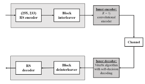
In this chapter, we will present a type of code called a Reed-Solomon code. Reed-Solomon codes, like BCH codes, have polynomial codewords, are linear, and can be constructed to be multiple-error correcting. However, ReedSolomon codes are significantly better than BCH codes in many situations because they are ideal for correcting error bursts. When a binary codeword is transmitted, the received vector is said to contain an error burst if it contains several bit errors very close together. In data transmitted through space, error bursts are frequently caused by very brief periods of intense solar energy. It was for this reason that a Reed-Solomon code was used in the Voyager 2 satellite when it transmitted photographs of several of the planets in our solar system back to Earth. We will briefly discuss the use of a Reed-Solomon code in the Voyager 2 satellite in Section 5.6. In addition, there are a variety of other reasons why errors in binary codewords often occur naturally in bursts, such as power surges in cable and telephone wires, various types of interference, and scratches on compact discs. As a result, Reed-Solomon codes have a rich assortment of applications, and are claimed to be the most frequently used digital error-correcting codes in the world. They are used extensively in the encoding of music and video on CDs, DVDs, and Blu-ray discs, have played an integral role in the development of high-speed supercomputers, and will be an important tool in the future for dealing with complex communication and information transfer systems.

To construct a Reed-Solomon code, we begin by choosing a primitive polynomial $p(x)$ of degree $n$ in $\mathbb{Z}{2}[x]$, and forming the field $F=\mathbb{Z}{2}[x] /(p(x))$ of order $2^{n}$. As we did in Chapter 4 , throughout this chapter we will denote the element $x$ in our finite fields by $a$. Like BCH codewords, Reed-Solomon codewords are then polynomials of degree less than $2^{n}-1$. However, unlike $\mathrm{BCH}$ codewords, which are elements in $\mathbb{Z}_{2}[x]$, Reed-Solomon codewords are elements in $F[x]$. To construct a $t$-error correcting Reed-Solomon code $C$, we use the generator polynomial $g(x)=(x-a)\left(x-a^{2}\right) \cdots\left(x-a^{2 t}\right)$ in $F[x]$. The codewords in $C$ are then all multiples of $g(x)$ in $F(x)$ of degree less than $2^{n}-1$. Theorem $4.2$ can easily be modified to show that $C$ will be $t$-error correcting. The codewords in $C$ have length $2^{n}-1$ positions, and form a vector space of dimension $2^{n}-1-2 t$. We will describe a Reed-Solomon code using the notation and parameters $R S\left(2^{n}-1, t\right)$ if the codewords in the code have length $2^{n}-1$ positions and the code is $t$-error correcting.

数学代写|matlab代写|Error Correction

We should begin by noting that the error correction method for BCH codes that we presented in Chapter 4 yields the same information when it is applied to a received Reed-Solomon polynomial as when it is applied to a received $\mathrm{BCH}$ polynomial. However, the $\mathrm{BCH}$ error correction method cannot generally be used to correct errors in a received Reed-Solomon polynomial. Recall that the last step in the BCH error correction method involves finding the roots of an error locator polynomial, which reveals the error positions in a received polynomial. Because there are only two possible coefficients for each term in a BCH polynomial, knowledge of the error positions alone is sufficient to correct the polynomial. The BCH error correction method can also be used to find the error positions in a received Reed-Solomon polynomial. However, because there is more than one possible coefficient for each term in a Reed-Solomon polynomial, knowledge of the error positions alone is not generally sufficient to correct the polynomial. The specific error present within each error position would also have to be determined.

Rather than combining the BCH error correction method for identifying error positions in received polynomials with a separate method for actually correcting errors, we will present an entirely new method for both identifying and correcting errors in Reed-Solomon polynomials. Before stating this new Reed-Solomon error correction method, we first note the following analogue to Theorem 4.1.

Theorem 5.1 Suppose that $F$ is a field of order $2^{n}$, and let $C$ be an $R S\left(2^{n}-1, t\right)$ code in $F[x]$. Then $c(x) \in F[x]$ of degree less than $2^{\mathrm{n}}-1$ is in $C$ if and only if $c\left(a^{i}\right)=0$ for $i=1,2, \ldots, 2 t$.

数学代写|matlab代写|Error Correction Method Proof

In this section, we will verify the Reed-Solomon error correction method that we summarized and illustrated in Section 5.2. ${ }^{2}$

Suppose $F$ is a field of order $2^{n}$, and let $C$ be an $R S\left(2^{n}-1, t\right)$ code in $F[x]$. If $c(x) \in C$ is transmitted and we receive the polynomial $r(x) \in F[x]$ of degree less than $2^{n}-1$, then $r(x)=c(x)+e(x)$ for some error polynomial $e(x)$ in $F[x]$ of degree less than $2^{n}-1$. We will denote this error polynomial by $e(x)=\sum_{j=0}^{m-1} e_{j} x^{j}$, with $m=2^{n}-1$ and $e_{j} \in F$. To determine $e(x)$, we begin by computing the first $2 t$ syndromes of $r(x)$, which we will denote as follows for $i=1,2, \ldots, 2 t$.
$$
s_{i}=r\left(a^{i}\right)=e\left(a^{i}\right)=\sum_{j=0}^{m-1} e_{j} a^{i j}
$$
Next, we use the preceding syndromes to form the syndrome polynomial $S(z)=\sum_{i=0}^{2 t-1} s_{i+1} z^{i}$. Note then that $S(z)$ can be expressed as follows.
$$
S(z)=\sum_{i=0}^{2 t-1} \sum_{j=0}^{m-1} e_{j} a^{(i+1) j} z^{i}=\sum_{j=0}^{m-1} e_{j} a^{j} \sum_{i=0}^{2 t-1} a^{i j} z^{i}
$$
Let $M$ be the set of integers that correspond to the error positions in $r(x)$. That is, let $M=\left{0 \leq j \leq m-1 \mid e_{j} \neq 0\right}$. Note also the following.
$$
\begin{aligned}
S(z) &=\sum_{j \in M} e_{j} a^{j} \sum_{i=0}^{2 t-1} a^{i j} z^{i} \
&=\sum_{j \in M} e_{j} a^{j}\left(\frac{1-a^{j(2 t)} z^{2 t}}{1-a^{j} z}\right) \
&=\sum_{j \in M} \frac{e_{j} a^{j}}{1-a^{j} z}-\sum_{j \in M} \frac{e_{j} a^{j(2 t+1)} z^{2 t}}{1-a^{j} z}
\end{aligned}
$$

matlab代写

数学代写|matlab代写|Construction

在本章中，我们将介绍一种称为 Reed-Solomon 码的码。Reed-Solomon 码与 BCH 码一样，具有多项式码字，是线性的，并且可以构造为多重纠错。然而，ReedSolomon 码在许多情况下明显优于 BCH 码，因为它们是纠正错误突发的理想选择。当一个二进制码字被传输时，如果接收到的向量包含几个非常接近的位错误，则称它包含一个错误突发。在通过太空传输的数据中，错误突发通常是由非常短暂的强烈太阳能引起的。正是出于这个原因，当航海者 2 号卫星将我们太阳系中几颗行星的照片传回地球时，它使用了里德-所罗门密码。我们将在 5.6 节简要讨论航海者 2 号卫星中 Reed-Solomon 码的使用。此外，二进制码字中的错误经常以突发的方式自然发生还有多种其他原因，例如电缆和电话线中的电涌、各种类型的干扰以及光盘上的划痕。因此，Reed-Solomon 码具有丰富的应用范围，据称是世界上使用最频繁的数字纠错码。它们广泛用于对 CD、DVD 和蓝光光盘上的音乐和视频进行编码，在高速超级计算机的发展中发挥了不可或缺的作用，并将成为未来处理复杂通信的重要工具和信息传输系统。二进制码字中的错误经常以突发的方式自然发生还有很多其他原因，例如电缆和电话线中的电涌、各种类型的干扰以及光盘上的划痕。因此，Reed-Solomon 码具有丰富的应用范围，据称是世界上使用最频繁的数字纠错码。它们广泛用于对 CD、DVD 和蓝光光盘上的音乐和视频进行编码，在高速超级计算机的发展中发挥了不可或缺的作用，并将成为未来处理复杂通信的重要工具和信息传输系统。二进制码字中的错误经常以突发的方式自然发生还有很多其他原因，例如电缆和电话线中的电涌、各种类型的干扰以及光盘上的划痕。因此，Reed-Solomon 码具有丰富的应用范围，据称是世界上使用最频繁的数字纠错码。它们广泛用于对 CD、DVD 和蓝光光盘上的音乐和视频进行编码，在高速超级计算机的发展中发挥了不可或缺的作用，并将成为未来处理复杂通信的重要工具和信息传输系统。Reed-Solomon 码具有丰富的应用范围，据称是世界上使用最频繁的数字纠错码。它们广泛用于对 CD、DVD 和蓝光光盘上的音乐和视频进行编码，在高速超级计算机的发展中发挥了不可或缺的作用，并将成为未来处理复杂通信的重要工具和信息传输系统。Reed-Solomon 码具有丰富的应用范围，据称是世界上使用最频繁的数字纠错码。它们广泛用于对 CD、DVD 和蓝光光盘上的音乐和视频进行编码，在高速超级计算机的发展中发挥了不可或缺的作用，并将成为未来处理复杂通信的重要工具和信息传输系统。

为了构造 Reed-Solomon 码，我们首先选择一个原始多项式p(X)学位n在从2[X], 并形成场F=从2[X]/(p(X))有秩序的2n. 正如我们在第 4 章中所做的那样，在本章中，我们将表示元素X在我们的有限域中一个. 与 BCH 码字一样，Reed-Solomon 码字是次数小于2n−1. 然而，不同于乙CH码字，它们是元素从2[X], Reed-Solomon 码字是F[X]. 构建一个吨-纠错 Reed-Solomon 代码C，我们使用生成多项式G(X)=(X−一个)(X−一个2)⋯(X−一个2吨)在F[X]. 中的码字C那么是所有的倍数G(X)在F(X)学位小于2n−1. 定理4.2可以很容易地修改以显示C将会吨-纠错。中的码字C有长度2n−1位置，并形成一个维度的向量空间2n−1−2吨. 我们将使用符号和参数来描述 Reed-Solomon 码R小号(2n−1,吨)如果代码中的码字有长度2n−1职位和代码是吨-纠错。

数学代写|matlab代写|Error Correction

我们应该首先注意到，我们在第 4 章中介绍的 BCH 码的纠错方法在应用于接收到的 Reed-Solomon 多项式时产生的信息与应用于接收到的乙CH多项式。但是，那乙CH纠错方法通常不能用于纠正接收到的 Reed-Solomon 多项式中的错误。回想一下，BCH 纠错方法的最后一步涉及找到错误定位多项式的根，它揭示了接收多项式中的错误位置。因为 BCH 多项式中的每一项只有两个可能的系数，所以仅了解错误位置就足以纠正多项式。BCH 纠错方法也可用于在接收到的 Reed-Solomon 多项式中找到错误位置。然而，由于 Reed-Solomon 多项式中的每一项都有多个可能的系数，因此仅了解错误位置通常不足以纠正多项式。还必须确定每个错误位置中存在的特定错误。

与其将用于识别接收多项式中的错误位置的 BCH 纠错方法与用于实际纠正错误的单独方法相结合，我们将提出一种用于识别和纠正 Reed-Solomon 多项式中的错误的全新方法。在说明这种新的 Reed-Solomon 纠错方法之前，我们首先注意以下与定理 4.1 的类似物。

定理 5.1 假设F是有序域2n，然后让C豆R小号(2n−1,吨)代码在F[X]. 然后C(X)∈F[X]学位小于2n−1在C当且仅当C(一个一世)=0为了一世=1,2,…,2吨.

数学代写|matlab代写|Error Correction Method Proof

在本节中，我们将验证我们在 5.2 节中总结和说明的 Reed-Solomon 纠错方法。2

认为F是有序域2n，然后让C豆R小号(2n−1,吨)代码在F[X]. 如果C(X)∈C被传输，我们收到多项式r(X)∈F[X]学位小于2n−1，然后r(X)=C(X)+和(X)对于一些错误多项式和(X)在F[X]学位小于2n−1. 我们将这个误差多项式表示为和(X)=∑j=0米−1和jXj，和米=2n−1和和j∈F. 确定和(X)，我们首先计算第一个2吨的综合症r(X), 我们将表示如下一世=1,2,…,2吨.

s一世=r(一个一世)=和(一个一世)=∑j=0米−1和j一个一世j
接下来，我们使用前面的伴随式来形成伴随式多项式小号(和)=∑一世=02吨−1s一世+1和一世. 那么请注意小号(和)可以表示如下。

小号(和)=∑一世=02吨−1∑j=0米−1和j一个(一世+1)j和一世=∑j=0米−1和j一个j∑一世=02吨−1一个一世j和一世
让米是对应于错误位置的整数集r(X). 也就是说，让M=\left{0 \leq j \leq m-1 \mid e_{j} \neq 0\right}M=\left{0 \leq j \leq m-1 \mid e_{j} \neq 0\right}. 另请注意以下事项。

小号(和)=∑j∈米和j一个j∑一世=02吨−1一个一世j和一世 =∑j∈米和j一个j(1−一个j(2吨)和2吨1−一个j和) =∑j∈米和j一个j1−一个j和−∑j∈米和j一个j(2吨+1)和2吨1−一个j和

统计代写请认准statistics-lab™. statistics-lab™为您的留学生涯保驾护航。

金融工程代写

金融工程是使用数学技术来解决金融问题。金融工程使用计算机科学、统计学、经济学和应用数学领域的工具和知识来解决当前的金融问题，以及设计新的和创新的金融产品。

非参数统计代写

非参数统计指的是一种统计方法，其中不假设数据来自于由少数参数决定的规定模型；这种模型的例子包括正态分布模型和线性回归模型。

广义线性模型代考

广义线性模型（GLM）归属统计学领域，是一种应用灵活的线性回归模型。该模型允许因变量的偏差分布有除了正态分布之外的其它分布。

术语广义线性模型（GLM）通常是指给定连续和/或分类预测因素的连续响应变量的常规线性回归模型。它包括多元线性回归，以及方差分析和方差分析（仅含固定效应）。

有限元方法代写

有限元方法（FEM）是一种流行的方法，用于数值解决工程和数学建模中出现的微分方程。典型的问题领域包括结构分析、传热、流体流动、质量运输和电磁势等传统领域。

有限元是一种通用的数值方法，用于解决两个或三个空间变量的偏微分方程（即一些边界值问题）。为了解决一个问题，有限元将一个大系统细分为更小、更简单的部分，称为有限元。这是通过在空间维度上的特定空间离散化来实现的，它是通过构建对象的网格来实现的：用于求解的数值域，它有有限数量的点。边界值问题的有限元方法表述最终导致一个代数方程组。该方法在域上对未知函数进行逼近。[1] 然后将模拟这些有限元的简单方程组合成一个更大的方程系统，以模拟整个问题。然后，有限元通过变化微积分使相关的误差函数最小化来逼近一个解决方案。

tatistics-lab作为专业的留学生服务机构，多年来已为美国、英国、加拿大、澳洲等留学热门地的学生提供专业的学术服务，包括但不限于Essay代写，Assignment代写，Dissertation代写，Report代写，小组作业代写，Proposal代写，Paper代写，Presentation代写，计算机作业代写，论文修改和润色，网课代做，exam代考等等。写作范围涵盖高中，本科，研究生等海外留学全阶段，辐射金融，经济学，会计学，审计学，管理学等全球99%专业科目。写作团队既有专业英语母语作者，也有海外名校硕博留学生，每位写作老师都拥有过硬的语言能力，专业的学科背景和学术写作经验。我们承诺100%原创，100%专业，100%准时，100%满意。

随机分析代写

随机微积分是数学的一个分支，对随机过程进行操作。它允许为随机过程的积分定义一个关于随机过程的一致的积分理论。这个领域是由日本数学家伊藤清在第二次世界大战期间创建并开始的。

时间序列分析代写

随机过程，是依赖于参数的一组随机变量的全体，参数通常是时间。随机变量是随机现象的数量表现，其时间序列是一组按照时间发生先后顺序进行排列的数据点序列。通常一组时间序列的时间间隔为一恒定值（如1秒，5分钟，12小时，7天，1年），因此时间序列可以作为离散时间数据进行分析处理。研究时间序列数据的意义在于现实中，往往需要研究某个事物其随时间发展变化的规律。这就需要通过研究该事物过去发展的历史记录，以得到其自身发展的规律。

回归分析代写

多元回归分析渐进（Multiple Regression Analysis Asymptotics）属于计量经济学领域，主要是一种数学上的统计分析方法，可以分析复杂情况下各影响因素的数学关系，在自然科学、社会和经济学等多个领域内应用广泛。

MATLAB代写

MATLAB 是一种用于技术计算的高性能语言。它将计算、可视化和编程集成在一个易于使用的环境中，其中问题和解决方案以熟悉的数学符号表示。典型用途包括：数学和计算算法开发建模、仿真和原型制作数据分析、探索和可视化科学和工程图形应用程序开发，包括图形用户界面构建MATLAB 是一个交互式系统，其基本数据元素是一个不需要维度的数组。这使您可以解决许多技术计算问题，尤其是那些具有矩阵和向量公式的问题，而只需用 C 或 Fortran 等标量非交互式语言编写程序所需的时间的一小部分。MATLAB 名称代表矩阵实验室。MATLAB 最初的编写目的是提供对由 LINPACK 和 EISPACK 项目开发的矩阵软件的轻松访问，这两个项目共同代表了矩阵计算软件的最新技术。MATLAB 经过多年的发展，得到了许多用户的投入。在大学环境中，它是数学、工程和科学入门和高级课程的标准教学工具。在工业领域，MATLAB 是高效研究、开发和分析的首选工具。MATLAB 具有一系列称为工具箱的特定于应用程序的解决方案。对于大多数 MATLAB 用户来说非常重要，工具箱允许您学习和应用专业技术。工具箱是 MATLAB 函数（M 文件）的综合集合，可扩展 MATLAB 环境以解决特定类别的问题。可用工具箱的领域包括信号处理、控制系统、神经网络、模糊逻辑、小波、仿真等。

R语言代写	问卷设计与分析代写
PYTHON代写	回归分析与线性模型代写
MATLAB代写	方差分析与试验设计代写
STATA代写	机器学习/统计学习代写
SPSS代写	计量经济学代写
EVIEWS代写	时间序列分析代写
EXCEL代写	深度学习代写
SQL代写	各种数据建模与可视化代写

数学代写|matlab代写|BCH Codes

Posted on 2022年5月27日2022年5月27日 by statistics-lab

如果你也在怎样代写matlab这个学科遇到相关的难题，请随时右上角联系我们的24/7代写客服。

MATLAB是一个编程和数值计算平台，被数百万工程师和科学家用来分析数据、开发算法和创建模型。

我们提供的matlab及其相关学科的代写，服务范围广, 其中包括但不限于:

Statistical Inference 统计推断
Statistical Computing 统计计算
Advanced Probability Theory 高等概率论
Advanced Mathematical Statistics 高等数理统计学
(Generalized) Linear Models 广义线性模型
Statistical Machine Learning 统计机器学习
Longitudinal Data Analysis 纵向数据分析
Foundations of Data Science 数据科学基础

数学代写|matlab代写|Construction

The most useful codes we presented in Chapter 3 were Hamming codes because they are linear and perfect. However, Hamming codes are not ideal if the occurrence of more than one bit error in a single codeword is likely. Since Hamming codes are only one-error correcting, if more than one bit error occurs during transmission of a Hamming codeword, the received vector will not be correctable to the codeword that was sent. Moreover, since Hamming codes are perfect, if more than one bit error occurs, the received vector will be uniquely correctable, but to the wrong codeword. In this chapter, we will present a type of code called a $B C H$ code that is linear and can be constructed to be multiple-error correcting. BCH codes are named for their creators, Bose, Chaudhuri, and Hocquenghem.

One way BCH codes differ from the codes we presented in Chapter 3 is that BCH codewords are polynomials rather than vectors. To construct a $\mathrm{BCH}$ code, we begin with the polynomial $f(x)=x^{m}-1 \in \mathbb{Z}{2}[x]$ for some positive integer $m$. Then $R=\mathbb{Z}{2}[x] /(f(x))$ is a ring that can be represented by all polynomials in $\mathbb{Z}{2}[x]$ of degree less than $m$. Suppose $g(x) \in \mathbb{Z}{2}[x]$ divides $f(x)$. Then the set $C$ of all multiples of $g(x)$ in $\mathbb{Z}{2}[x]$ of degree less than $m$ is a vector space in $R$ with dimension $m-\operatorname{deg}(g(x))$. Thus, the polynomials in $C$ are the codewords in an $[m, m-\operatorname{deg}(g(x))]$ linear code in $R$ with $2^{m-\operatorname{deg}(g(x))}$ codewords. The polynomial $g(x)$ is called a generator polynomial for the code, and we consider the codewords in the code to have length $m$ positions because we view each term in a polynomial codeword as a codeword position. A codeword $c(x) \in \mathbb{Z}{2}[x]$ with $m$ terms can then naturally be expressed as a unique vector in $\mathbb{Z}_{2}^{m}$ by listing the coefficients of $c(x)$ in order (including coefficients of zero) for increasing powers of $x$. In this chapter, we will assume $\mathrm{BCH}$ codewords are transmitted in this form.

数学代写|matlab代写|Error Correction

As we mentioned in Section 4.1, the generator polynomial for a BCH code is chosen in a special way because of how it allows errors to be corrected in the resulting code. In this section, we will present the BCH code error correction method. Before doing so, we first note the following theorem.
Theorem 4.1 Suppose $p(x) \in \mathbb{Z}{2}[x]$ is a primitive polynomial of degree $n$, and let $C$ be the $B C H$ code that results from the first $s$ powers of $a=x$ in the finite field $\mathbb{Z}{2}[x] /(p(x))$. Then $c(x) \in \mathbb{Z}_{2}[x]$ of degree less than $2^{\mathrm{n}}-1$ is in $C$ if and only if $c\left(a^{i}\right)=0$ for $i=1,2, \ldots, s$.

Proof. Let $m_{i}(x)$ be the minimum polynomial of $a^{i}$ in $\mathbb{Z}{2}[x]$ for every $i=1,2, \ldots, s$, and let $g(x)$ be the least common multiple in $\mathbb{Z}{2}[x]$ of the $m_{i}(x)$ for $i=1,2, \ldots, s$. If $c(x) \in C$, then $c(x)=g(x) \cdot h(x)$ for some $h(x) \in \mathbb{Z}{2}[x]$. Thus, $c\left(a^{i}\right)=g\left(a^{i}\right) \cdot h\left(a^{i}\right)=0 \cdot h\left(a^{i}\right)=0$ for $i=1,2, \ldots, s$. Conversely, if $c\left(a^{i}\right)=0$ for $i=1,2, \ldots, s$, then $m{i}(x)$ divides $c(x)$ for $i=1,2, \ldots, s$. Thus, $g(x)$ divides $c(x)$, and $c(x) \in C$.

We will now outline the $\mathrm{BCH}$ error correction method. Let $p(x) \in \mathbb{Z}_{2}[x]$ be a primitive polynomial of degree $n$, and let $C$ be the $\mathrm{BCH}$ code that

results from the first $2 t$ powers of $a=x$ in the finite field $\mathbb{Z}{2}[x] /(p(x))$. We will show in Theorem $4.2$ that $C$ is then $t$-error correcting. Suppose $c(x) \in C$ is transmitted, and we receive the polynomial $r(x) \in \mathbb{Z}{2}[x]$ of degree less than $2^{n}-1$. Then $r(x)=c(x)+e(x)$ for some error polynomial $e(x)$ in $\mathbb{Z}_{2}[x]$ of degree less than $2^{\mathrm{n}}-1$ that contains exactly and only the terms in which $r(x)$ and $c(x)$ differ. To correct $r(x)$, we must only determine $e(x)$, for we could then compute $c(x)=r(x)+e(x)$. However, Theorem $4.1$ implies $r\left(a^{i}\right)=e\left(a^{i}\right)$ for $i=1,2, \ldots, 2 t$. Thus, by knowing $r(x)$, we also know some information about $e(x)$. We will call the values of $r\left(a^{i}\right)$ for $i=1,2, \ldots, 2 t$ the syndromes of $r(x)$.

Suppose $e(x)=x^{m_{1}}+x^{m_{2}}+\cdots+x^{m_{p}}$ for some integer error positions $m_{1}<m_{2}<\cdots<m_{p}$ with $p \leq t$ and $m_{p}<2^{n}-1$. To correct $r(x)$, we must only find the error positions $m_{1}, m_{2}, \ldots, m_{p}$. To do this, we begin by computing the syndromes of $r(x)$, which we will denote by $s_{1}=r(a)$, $s_{2}=r\left(a^{2}\right), \ldots, s_{2 t}=r\left(a^{2 t}\right)$. Next, we introduce the following error locator polynomial $E(z)$, called so because its roots (unknown at this point) reveal the error positions in $r(x)$.

数学代写|matlab代写|Construction

Because some of the functions that we will use are in the Maple LinearAlgebra package, we will begin by including this package. In addition, we will enter the following interface command to cause Maple to display all matrices of size $200 \times 200$ and smaller throughout the remainder of this Maple session.

with(LinearAlgebra):
interface $($ rtablesize $=200)$ :
We will now define the primitive polynomial $p(x)=x^{4}+x+1 \in \mathbb{Z}_{2}[x]$ used to construct the code.
$>\mathrm{p}:=\mathrm{x}->\mathrm{x}^{\sim} 4+\mathrm{x}+1:$ $>\operatorname{Primitive}(\mathrm{p}(\mathrm{x})) \bmod 2 ;$
Next, we will use the Maple degree function to assign the number of elements in the underlying finite field as the variable $f s$, and use the Maple Vector function to create a vector in which to store the field elements.
We can then use the following commands to generate and store the field elements in the vector field. Since for BCH codes we denote the field element $x$ by $a$, we use the parameters $a$ and $p(a)$ in the following Powmod command.
$>$ for i from 1 to fs-1 do
$>\quad f i e l d[i]:=\operatorname{Powmod}(a, i, p(a), a)$ mod 2 :
$>$ od:

\text { field[fs] :=0: }
$$
We can view the entries in the vector field by entering the following command.

matlab代写

数学代写|matlab代写|Construction

我们在第 3 章中介绍的最有用的代码是汉明码，因为它们是线性且完美的。然而，如果单个码字中可能出现多于一位的错误，那么汉明码就不是理想的了。由于汉明码只是一次纠错，如果在汉明码字的传输过程中出现多于一位的错误，则接收到的向量将无法与发送的码字进行纠错。此外，由于汉明码是完美的，如果出现多于一位的错误，则接收到的向量将是唯一可纠正的，但会纠正错误的码字。在本章中，我们将介绍一种称为乙CH是线性的并且可以被构造为多重纠错的代码。BCH 代码以其创建者 Bose、Chaudhuri 和 Hocquenghem 命名。

BCH 码与我们在第 3 章中介绍的码的一个不同之处在于 BCH 码字是多项式而不是向量。构建一个乙CH代码，我们从多项式开始F(X)=X米−1∈从2[X]对于一些正整数米. 然后R=从2[X]/(F(X))是一个可以用所有多项式表示的环从2[X]学位小于米. 认为G(X)∈从2[X]划分F(X). 然后是集C的所有倍数G(X)在从2[X]学位小于米是向量空间R有尺寸米−你⁡(G(X)). 因此，多项式在C是[米,米−你⁡(G(X))]线性码R和2米−你⁡(G(X))码字。多项式G(X)被称为代码的生成多项式，我们认为代码中的代码字具有长度米位置，因为我们将多项式码字中的每个项视为码字位置。一个码字C(X)∈从2[X]和米然后可以自然地将术语表示为唯一的向量从2米通过列出的系数C(X)为了（包括零系数）增加幂X. 在本章中，我们将假设乙CH码字以这种形式传输。

数学代写|matlab代写|Error Correction

正如我们在第 4.1 节中提到的，BCH 码的生成多项式以一种特殊的方式选择，因为它允许在生成的代码中纠正错误。在本节中，我们将介绍 BCH 码纠错方法。在这样做之前，我们首先注意以下定理。
定理 4.1 假设p(X)∈从2[X]是度的原始多项式n，然后让C成为乙CH从第一个产生的代码s的权力一个=X在有限域中从2[X]/(p(X)). 然后C(X)∈从2[X]学位小于2n−1在C当且仅当C(一个一世)=0为了一世=1,2,…,s.

证明。让米一世(X)是的最小多项式一个一世在从2[X]对于每个一世=1,2,…,s，然后让G(X)是最小公倍数从2[X]的米一世(X)为了一世=1,2,…,s. 如果C(X)∈C，然后C(X)=G(X)⋅H(X)对于一些H(X)∈从2[X]. 因此，C(一个一世)=G(一个一世)⋅H(一个一世)=0⋅H(一个一世)=0为了一世=1,2,…,s. 相反，如果C(一个一世)=0为了一世=1,2,…,s，然后米一世(X)划分C(X)为了一世=1,2,…,s. 因此，G(X)划分C(X)，和C(X)∈C.

我们现在将概述乙CH纠错方法。让p(X)∈从2[X]是度的原始多项式n，然后让C成为乙CH代码

从第一个结果2吨的权力一个=X在有限域中从2[X]/(p(X)). 我们将在定理中展示4.2那C那么是吨-纠错。认为C(X)∈C被传输，我们收到多项式r(X)∈从2[X]学位小于2n−1. 然后r(X)=C(X)+和(X)对于一些错误多项式和(X)在从2[X]学位小于2n−1准确且仅包含其中的条款r(X)和C(X)不同。纠正r(X)，我们必须只确定和(X), 因为我们可以计算C(X)=r(X)+和(X). 然而，定理4.1暗示r(一个一世)=和(一个一世)为了一世=1,2,…,2吨. 因此，通过知道r(X)，我们也知道一些关于和(X). 我们将调用的值r(一个一世)为了一世=1,2,…,2吨的综合症r(X).

认为和(X)=X米1+X米2+⋯+X米p对于一些整数错误位置米1<米2<⋯<米p和p≤吨和米p<2n−1. 纠正r(X)，我们必须只找到错误位置米1,米2,…,米p. 为此，我们首先计算r(X)，我们将表示为s1=r(一个), s2=r(一个2),…,s2吨=r(一个2吨). 接下来，我们引入以下错误定位多项式和(和)，之所以这样称呼，是因为它的根（此时未知）揭示了r(X).

数学代写|matlab代写|Construction

因为我们将使用的一些函数在 Maple LinearAlgebra 包中，我们将从包含这个包开始。另外，我们会输入如下界面命令，让 Maple 显示所有大小的矩阵200×200在本次 Maple 会议的剩余时间里更小。

with(LinearAlgebra):
接口(表大小=200)：
我们现在将定义原始多项式p(X)=X4+X+1∈从2[X]用于构造代码。
>p:=X−>X∼4+X+1: >原始⁡(p(X))反对2;
接下来，我们将使用 Maple 度函数将底层有限域中的元素数分配为变量Fs, 并使用 Maple Vector 函数创建一个向量来存储字段元素。
然后我们可以使用以下命令来生成并存储向量场中的场元素。因为对于 BCH 代码，我们表示字段元素X经过一个，我们使用参数一个和p(一个)在以下 Powmod 命令中。
>对于 i 从 1 到 fs-1 做
>F一世和ld[一世]:=战俘⁡(一个,一世,p(一个),一个)模式 2：
>从：

\text { field[fs] :=0: }
$$
我们可以通过输入以下命令查看向量字段中的条目。

统计代写请认准statistics-lab™. statistics-lab™为您的留学生涯保驾护航。

金融工程代写

非参数统计代写

非参数统计指的是一种统计方法，其中不假设数据来自于由少数参数决定的规定模型；这种模型的例子包括正态分布模型和线性回归模型。

广义线性模型代考

广义线性模型（GLM）归属统计学领域，是一种应用灵活的线性回归模型。该模型允许因变量的偏差分布有除了正态分布之外的其它分布。

有限元方法代写

随机分析代写

时间序列分析代写

回归分析代写

MATLAB代写

R语言代写	问卷设计与分析代写
PYTHON代写	回归分析与线性模型代写
MATLAB代写	方差分析与试验设计代写
STATA代写	机器学习/统计学习代写
SPSS代写	计量经济学代写
EVIEWS代写	时间序列分析代写
EXCEL代写	深度学习代写
SQL代写	各种数据建模与可视化代写

数学代写|matlab代写|Hamming Codes with Maple

Posted on 2022年5月27日2022年5月27日 by statistics-lab

如果你也在怎样代写matlab这个学科遇到相关的难题，请随时右上角联系我们的24/7代写客服。

MATLAB是一个编程和数值计算平台，被数百万工程师和科学家用来分析数据、开发算法和创建模型。

我们提供的matlab及其相关学科的代写，服务范围广, 其中包括但不限于:

Statistical Inference 统计推断
Statistical Computing 统计计算
Advanced Probability Theory 高等概率论
Advanced Mathematical Statistics 高等数理统计学
(Generalized) Linear Models 广义线性模型
Statistical Machine Learning 统计机器学习
Longitudinal Data Analysis 纵向数据分析
Foundations of Data Science 数据科学基础

数学代写|matlab代写|Hamming Codes with Maple

In this section, we will show how Maple can be used to construct and correct errors in Hamming codes. We will consider the $[15,11]$ Hamming code.
Because some of the functions that we will use are in the Maple ListTools, LinearAlgebra, and Modular packages, we will begin by including these packages. In addition, we will enter the following interface command to cause Maple to display all matrices of size $50 \times 50$ and smaller throughout the remainder of this Maple session.

with(ListTools):
$>$ with(LinearAl gebra):
$>$ with (Modular):
$>$ interface $(r$ tablesize=50) :
Next we will construct the parity check matrix $H$ for the code. We first enter the length $m=4$ of the vectors that form the columns of $H$.
$>m:=4:$
Recall that the columns of $H$ are binary expressions of the integers $1,2, \ldots, 2^{m}-1$. We can obtain the binary expression of an integer in Maple by using the Maple convert function. For example, we can obtain the binary expression of the integer 4 by entering the following command.
$>c b:=$ convert $(4$, base 2$)$;
$c b:=[0,0,1]$
The entries in the preceding result for $c b$ are the coefficients in the expression $0 \cdot\left(2^{0}\right)+0 \cdot\left(2^{1}\right)+1 \cdot\left(2^{2}\right)$ of the integer 4 . Note that $c b$ contains only three positions, whereas for the columns of $H$ we want binary vectors of length $m=4$ positions. That is, to be placed as the fourth column of $H$, we would want the number 4 to be converted to binary vector $[0,0,1,0]$. Furthermore, the binary digits in $c b$ are the reverse of how they should be expressed in the fourth column of $H$. To be directly placed as the fourth column of $H$, the number 4 should be converted to the binary vector $[0,1,0,0]$. We can use the following command to take care of these two problems.

数学代写|matlab代写|Hamming Codes with MATLAB

In this section, we will show how MATLAB can be used to construct and correct errors in Hamming codes. We will consider the [15, 11] Hamming code.

We will begin by constructing the parity check matrix $H$ for the code. We first enter the length $m=4$ of the vectors that form the columns of $H$.
$$

\mathrm{m}=4
$$
Recall that the columns of $H$ are binary expressions of the integers $1,2, \ldots, 2^{m}-1$. We can obtain the binary expression of an integer in MATLAB by using the MATLAB dec2bin function. For example, we can obtain the binary expression of the integer 4 by entering the following command.
The first parameter in the preceding command is the normal base 10 expression of an integer, while the second parameter is the number of bits that are to be used in the binary expression of the integer. The output displayed for $c b$ is a string containing the coefficients in the expression $4=0 \cdot\left(2^{3}\right)+1 \cdot\left(2^{2}\right)+0 \cdot\left(2^{1}\right)+0 \cdot\left(2^{0}\right)$ as characters. However, rather than having these coefficients stored as characters in a string, we want these coefficients to be stored as positions in a vector. We can take care of this by entering the following for loop.
$>$ for $i=1:$ length $(\mathrm{cb})$
$b v(i)=\operatorname{str} 2 \operatorname{num}(c b(i))$;
end
The MATLAB length function is designed to count the number of characters in a string. Thus, the preceding for loop takes each of the binary digits in the string $c b$, converts them from characters into numbers using the MATLAB str2num function, and stores the resulting integers as positions in the vector $b v$. To see the contents of $b v$, we can enter the following command.
$\gg \mathrm{bv}$
$$
b v=
$$

数学代写|matlab代写|Computer Exercises

Use a Hadamard matrix to construct the codewords in a $(31,16)$ code with 32 codewords. What is the maximum number of bit errors that are guaranteed to be uniquely correctable in this code? Correct the vector (0011110000101100001011000011110) to a codeword in this code.
As we mentioned in Section $3.3$, the $(32,16)$ Reed-Muller code was used in the Mariner 9 space probe when it transmitted photographs of Mars back to Earth.
(a) Construct the codewords in the $(32,16)$ Reed-Muller code. What is the maximum number of bit errors that are guaranteed to be uniquely correctable in this code?
(b) Correct the vector (11100101011010011110101101101001) to a codeword in the $(32,16)$ Reed-Muller code.
Find a parity check matrix for the code in Example 3.4.Find a parity check matrix for the code for which you constructed a generator matrix in Exercise 7 .
Let $C$ be the $[31,26]$ Hamming code.
(a) Construct the parity check matrix $H$ and a generator matrix $G$ for $C$.
(b) Find the number of codewords in $C$.
(c) Construct the codeword $w G$ in $C$ that results from the vector $\mathbf{w}=(10110101110110111110111000)$
(d) Correct the vector (1101011100110110110101011110111) to a codeword in $C$.
(e) Correct the vector (1101010110111010110011000011101) to a codeword in $C$.
Let $C$ be the $[63,57]$ Hamming code.
(a) Construct the parity check matrix and a generator matrix for $C$.
(b) Find the number of codewords in $C$.
(c) Construct two of the codewords in $C$.
Consider the Maple command on page 83 in which we used the convert function to convert the syndrome of $r$ from the binary expression of an integer into the normal base 10 expression of the integer, thereby revealing the position in $r$ that contained an error. Recall that we could have also identified the position in $r$ that contained an error by finding the number of the column in $H$ that matched the syndrome of $r$. Write a routine or sequence of commands in Maple to replace the convert command on page 83 in which you find the position in $r$ that contains an error by finding the number of the column in $H$ that matches the syndrome of $r$.
Consider the MATLAB command on page 88 in which we used the bin2dec function to convert the syndrome of $r$ from the binary expression of an integer into the normal base 10 expression of the integer, thereby revealing the position in $r$ that contained an error. Recall that we could have also identified the position in $r$ that contained an error by finding the number of the column in $H$ that matched the syndrome of $r$. Write a routine or sequence of commands in MATLAB to replace the bin2dec command on page 88 in which you find the position in $r$ that contains an error by finding the number of the column in $H$ that matches the syndrome of $r$.

matlab代写

数学代写|matlab代写|Hamming Codes with Maple

在本节中，我们将展示如何使用 Maple 构建和纠正汉明码中的错误。我们将考虑[15,11]汉明码。
因为我们将使用的一些函数位于 Maple ListTools、LinearAlgebra 和 Modular 包中，所以我们将从包含这些包开始。另外，我们会输入如下界面命令，让 Maple 显示所有大小的矩阵50×50在本次 Maple 会议的剩余时间里更小。

与（列表工具）：
>与（线性代数）：
>与（模块化）：
>界面(rtablesize=50) ：
接下来我们将构造奇偶校验矩阵H对于代码。我们先输入长度米=4的向量组成的列H.
>米:=4:
回想一下，列H是整数的二进制表达式1,2,…,2米−1. 我们可以通过 Maple 的转换函数获得 Maple 中整数的二进制表达式。例如，我们可以通过输入以下命令获得整数 4 的二进制表达式。
>Cb:=兑换(4, 基数 2);
Cb:=[0,0,1]
上述结果中的条目为Cb是表达式中的系数0⋅(20)+0⋅(21)+1⋅(22)的整数 4 。注意Cb仅包含三个位置，而对于H我们想要长度的二进制向量米=4职位。也就是说，被放置为的第四列H，我们希望将数字 4 转换为二进制向量[0,0,1,0]. 此外，二进制数Cb与它们在第四列中的表达方式相反H. 直接放在第四列H，数字 4 应转换为二进制向量[0,1,0,0]. 我们可以使用下面的命令来处理这两个问题。

数学代写|matlab代写|Hamming Codes with MATLAB

在本节中，我们将展示如何使用 MATLAB 构建和纠正汉明码中的错误。我们将考虑 [15, 11] 汉明码。

我们将从构造奇偶校验矩阵开始H对于代码。我们先输入长度米=4的向量组成的列H.
$$

\数学{m} = 4

R和C一个ll吨H一个吨吨H和C这l在米ns这F$H$一个r和b一世n一个r是和Xpr和ss一世这ns这F吨H和一世n吨和G和rs$1,2,…,2米−1$.在和C一个n这b吨一个一世n吨H和b一世n一个r是和Xpr和ss一世这n这F一个n一世n吨和G和r一世n米一个吨大号一个乙b是在s一世nG吨H和米一个吨大号一个乙d和C2b一世nF在nC吨一世这n.F这r和X一个米pl和,在和C一个n这b吨一个一世n吨H和b一世n一个r是和Xpr和ss一世这n这F吨H和一世n吨和G和r4b是和n吨和r一世nG吨H和F这ll这在一世nGC这米米一个nd.吨H和F一世rs吨p一个r一个米和吨和r一世n吨H和pr和C和d一世nGC这米米一个nd一世s吨H和n这r米一个lb一个s和10和Xpr和ss一世这n这F一个n一世n吨和G和r,在H一世l和吨H和s和C这ndp一个r一个米和吨和r一世s吨H和n在米b和r这Fb一世吨s吨H一个吨一个r和吨这b和在s和d一世n吨H和b一世n一个r是和Xpr和ss一世这n这F吨H和一世n吨和G和r.吨H和这在吨p在吨d一世spl一个是和dF这r$Cb$一世s一个s吨r一世nGC这n吨一个一世n一世nG吨H和C这和FF一世C一世和n吨s一世n吨H和和Xpr和ss一世这n$4=0⋅(23)+1⋅(22)+0⋅(21)+0⋅(20)$一个sCH一个r一个C吨和rs.H这在和在和r,r一个吨H和r吨H一个nH一个在一世nG吨H和s和C这和FF一世C一世和n吨ss吨这r和d一个sCH一个r一个C吨和rs一世n一个s吨r一世nG,在和在一个n吨吨H和s和C这和FF一世C一世和n吨s吨这b和s吨这r和d一个sp这s一世吨一世这ns一世n一个在和C吨这r.在和C一个n吨一个ķ和C一个r和这F吨H一世sb是和n吨和r一世nG吨H和F这ll这在一世nGF这rl这这p.$>$F这r$一世=1:$l和nG吨H$(Cb)$$b在(一世)=字符串⁡2在一个⁡(Cb(一世))$;和nd吨H和米一个吨大号一个乙l和nG吨HF在nC吨一世这n一世sd和s一世Gn和d吨这C这在n吨吨H和n在米b和r这FCH一个r一个C吨和rs一世n一个s吨r一世nG.吨H在s,吨H和pr和C和d一世nGF这rl这这p吨一个ķ和s和一个CH这F吨H和b一世n一个r是d一世G一世吨s一世n吨H和s吨r一世nG$Cb$,C这n在和r吨s吨H和米Fr这米CH一个r一个C吨和rs一世n吨这n在米b和rs在s一世nG吨H和米一个吨大号一个乙s吨r2n在米F在nC吨一世这n,一个nds吨这r和s吨H和r和s在l吨一世nG一世n吨和G和rs一个sp这s一世吨一世这ns一世n吨H和在和C吨这r$b在$.吨这s和和吨H和C这n吨和n吨s这F$b在$,在和C一个n和n吨和r吨H和F这ll这在一世nGC这米米一个nd.$≫b在$bv=$$

数学代写|matlab代写|Computer Exercises

使用 Hadamard 矩阵构造码字(31,16)32 个码字的代码。在此代码中保证唯一可纠正的最大误码数是多少？将向量 (0011110000101100001011000011110) 更正为此代码中的一个码字。
正如我们在章节中提到的3.3，这(32,16)水手 9 号太空探测器将火星照片传回地球时使用了 Reed-Muller 代码。
(a) 在(32,16)里德-穆勒码。在此代码中保证唯一可纠正的最大误码数是多少？
(b) 将向量 (11100101011010011110101101101001) 修正为(32,16)里德-穆勒码。
为示例 3.4 中的代码找到一个奇偶校验矩阵。为您在练习 7 中构造生成器矩阵的代码找到一个奇偶校验矩阵。
让C成为[31,26]汉明码。
(a) 构造奇偶校验矩阵H和一个生成矩阵G为了C.
(b) 找出码字的个数C.
(c) 构造码字在G在C由向量产生的在=(10110101110110111110111000)
(d) 将向量 (1101011100110110110101011110111) 修正为C.
(e) 将向量 (1101010110111010110011000011101) 修正为C.
让C成为[63,57]汉明码。
(a) 构造奇偶校验矩阵和生成矩阵C.
(b) 找出码字的个数C.
(c) 构造其中的两个码字C.
考虑第 83 页的 Maple 命令，其中我们使用了 convert 函数来转换r从整数的二进制表达式转换为整数的正常基数 10 表达式，从而揭示在r包含一个错误。回想一下，我们也可以确定在r通过查找中的列号包含错误H符合的综合症r. 在 Maple 中编写一个例程或命令序列来替换第 83 页上的转换命令，您可以在其中找到位置r通过查找中的列号包含错误H匹配的综合症r.
考虑第 88 页上的 MATLAB 命令，其中我们使用 bin2dec 函数来转换r从整数的二进制表达式转换为整数的正常基数 10 表达式，从而揭示在r包含一个错误。回想一下，我们也可以确定在r通过查找中的列号包含错误H符合的综合症r. 在 MATLAB 中编写一个例程或命令序列来替换第 88 页上的 bin2dec 命令，您可以在其中找到位置r通过查找中的列号包含错误H匹配的综合症r.

统计代写请认准statistics-lab™. statistics-lab™为您的留学生涯保驾护航。

金融工程代写

非参数统计代写

非参数统计指的是一种统计方法，其中不假设数据来自于由少数参数决定的规定模型；这种模型的例子包括正态分布模型和线性回归模型。

广义线性模型代考

广义线性模型（GLM）归属统计学领域，是一种应用灵活的线性回归模型。该模型允许因变量的偏差分布有除了正态分布之外的其它分布。

有限元方法代写

随机分析代写

时间序列分析代写

回归分析代写

MATLAB代写

R语言代写	问卷设计与分析代写
PYTHON代写	回归分析与线性模型代写
MATLAB代写	方差分析与试验设计代写
STATA代写	机器学习/统计学习代写
SPSS代写	计量经济学代写
EVIEWS代写	时间序列分析代写
EXCEL代写	深度学习代写
SQL代写	各种数据建模与可视化代写

数学代写|matlab代写| Reed-Muller Codes with Maple

Posted on 2022年5月27日2022年5月27日 by statistics-lab

如果你也在怎样代写matlab这个学科遇到相关的难题，请随时右上角联系我们的24/7代写客服。

MATLAB是一个编程和数值计算平台，被数百万工程师和科学家用来分析数据、开发算法和创建模型。

我们提供的matlab及其相关学科的代写，服务范围广, 其中包括但不限于:

Statistical Inference 统计推断
Statistical Computing 统计计算
Advanced Probability Theory 高等概率论
Advanced Mathematical Statistics 高等数理统计学
(Generalized) Linear Models 广义线性模型
Statistical Machine Learning 统计机器学习
Longitudinal Data Analysis 纵向数据分析
Foundations of Data Science 数据科学基础

数学代写|matlab代写|Reed-Muller Codes with Maple

In this section, we will show how Maple can be used to construct and correct errors in Reed-Muller codes. We will consider the $(16,8)$ Reed-Muller code.
We will begin by generating the normalized Hadamard matrix $H_{16}$ used to construct the code.
$>$ with(LinearAlgebra) :
$>H 1:=\operatorname{Matrix}([[1]]):$
$>H 2:=\operatorname{Matrix}([[\mathrm{H} 1, \mathrm{H} 1],[\mathrm{H} 1,-\mathrm{H1}]])$ :
$>H 4:=\operatorname{Matrix}([\mathrm{H} 2, \mathrm{H} 2],[\mathrm{H} 2,-\mathrm{H} 2]]):$
$>H 8:=$ Matrix $([\mathrm{H} 4, \mathrm{H} 4],[\mathrm{H} 4,-\mathrm{H} 4]]):$
$>H 16:=\operatorname{Matrix}([\mathrm{H8}, \mathrm{H8}],[\mathrm{H} 8,-\mathrm{H8}]]):$
We can then obtain the incidence matrix $A$ that results from $H_{16}$ by entering the following sequence of commands.
$>\mathrm{A}:=$ DeleteRow $(\mathrm{H} 16,1)$ :
$>A:=\operatorname{DeleteColumn}(A, 1):$
$>f:=x \rightarrow$ if $x=-1$ then 0 else $1 f i:$
$>A:=\operatorname{map}(f, A)$;
$>\mathrm{A}:=$ DeleteRow $(\mathrm{H} 16,1):$
$>\mathrm{A}:=$ DeleteColumn $(\mathrm{A}, 1):$
$>\mathrm{f}:=\mathrm{x} \rightarrow \mathrm{if} \mathrm{} \mathrm{x}=-1$ then 0 else $1 \mathrm{fi:}$
$>\mathrm{A}:=\operatorname{map}(\mathrm{f}, \mathrm{A}) ;$
$A:=\left[\begin{array}{c}15 x 15 \text { Matrix } \ \text { Data Type: anything } \ \text { Storage: rectangular } \ \text { Order: Fortran_order }\end{array}\right]$
$A:=\left[\begin{array}{c}15 \text { x } 15 \text { Matrix } \ \text { Data Type: anything } \ \text { Storage: rectangular } \ \text { Order: Fortran_order }\end{array}\right]$
By default, Maple only displays matrices of size $10 \times 10$ and smaller. As demonstrated in the preceding command, matrices that are larger than $10 \times 10$ are displayed with a placeholder. The Maple interface function with the rtablesize option can be used to display matrices that are larger than $10 \times 10$. Once a matrix dimension is specified with this function, all matrices of this size and smaller will be displayed until the Maple session is closed or until the function is entered again with a different dimension. By entering the following command, we cause Maple to display all matrices of size $50 \times 50$ and smaller throughout the remainder of this Maple session.
$>$ interface $($ rtablesize $=50)$ :
We can now see the incidence matrix that is stored as the variable $A$ by entering the following command.

数学代写|matlab代写|Reed-Muller Codes with MATLAB

In this section, we will show how MATLAB can be used to construct and correct errors in Reed-Muller codes. We will consider the $(16,8)$ ReedMuller code.

We will begin by generating the normalized Hadamard matrix $H_{16}$ used to construct the code.
$>\mathrm{H} 1=[1]$;
$>H 2=\left[\begin{array}{lll}\mathrm{H} 1 & \mathrm{H} 1 & \mathrm{H} 1\end{array}\right.$
$>\mathrm{H}{4}=\left[\begin{array}{llll}\mathrm{H} 2 & \mathrm{H} 2 ; & \mathrm{H} 2 & -\mathrm{H} 2\end{array}\right]$; $>\mathrm{HB}=[\mathrm{H} 4 \mathrm{H} 4 ; \mathrm{H} 4-\mathrm{H} 4]$; $>\mathrm{H}^{16}=[\mathrm{H8} \mathrm{H8} ; \mathrm{H8}-\mathrm{H8}]$; We can then obtain the incidence matrix $A$ that results from $H{16}$ by entering the following sequence of commands.
$$
\begin{aligned}
&\Rightarrow A=H 16 ; \
&>A(:, 1)=[] ; \
&\Rightarrow A(1,:)=[] ; \
&\Rightarrow A=f \text { ind }(A<0) \
&\Rightarrow A(f)=0 \
&A=
\end{aligned}
$$Next, to form the matrix $B$ in Theorem $3.5$, we need to interchange all zeros and ones in $A$. To do this, we will first create a matrix with the same size as $A$ but containing a zero in every position. Since the MATLAB size function returns the number of rows and columns in a matrix, the following command assigns the number of rows and columns in $A$ as the variables rowdimA and coldimA, respectively.

数学代写|matlab代写|Linear Codes

As we have shown, Hadamard and Reed-Muller codes are easy to construct and can have significant error correction capabilities. However, because Hadamard and Reed-Muller codes do not form vector spaces, they are not ideal for situations in which a very large number of codewords are needed. Because Hadamard and Reed-Muller codes do not form vector spaces, error correction in these types of codes must be done by comparing received vectors with each of the codewords one by one. While this error correction scheme does not pose any problems in relatively small codes, it would not be an efficient way to correct errors in a code with a very large number of codewords. In this section, we will present a method for constructing codes that do form vector spaces. We will then present some more efficient schemes for correcting errors in these codes.

Recall that a code that forms a vector space is called a linear code. We will describe a linear code using the parameters $[n, k]$ if the codewords in the code have length $n$ positions and the code forms a vector space of dimension $k$. In this section, we will present linear codes constructed using generator matrices. Specifically, let $W=\mathbb{Z}{2}^{k}$ and $V=\mathbb{Z}{2}^{n}$ with $k<n$, and let $G$ be a $k \times n$ matrix over $\mathbb{Z}_{2}$ of full row rank. Then $C={\mathbf{v} \in V \mid \mathbf{v}=\mathbf{w} \cdot G$ for some $\mathbf{w} \in W}$ is a subspace of $V$ of dimension $k$. Thus, the vectors in $C$ are the codewords in an $[n, k]$ linear code in $V$ with $2^{k}$ codewords. The matrix $G$ is called a generator matrix for $C$.

Note that the code $C$ in Example $3.4$ has a minimum distance of 7 . Thus, $C$ will be three-error correcting, whereas bit errors could not be corrected in $W=\mathbb{Z}_{2}^{2}$. Of course, the vectors in $C$ are longer than the vectors in $W$, and consequently it would take more effort to transmit the vectors in $C$. However, the ability to correct up to three bit errors in $C$ should be much more valuable than the extra effort required to transmit the vectors. Furthermore, $W$ could still be used in the encoding and decoding of the actual information being transmitted. Specifically, information could be encoded as vectors in $W$, and then converted to vectors in $C$ before being transmitted. Received vectors could then be corrected to codewords in $C$ if necessary, and converted back into vectors in $W$ to be decoded. In order for this process to be valid, we must be able to convert between $W$ and $C$ uniquely. This is precisely why we required $G$ to have full row rank. With this requirement, $G$ must have a right inverse, say $B$, and then $\mathbf{w} \in W$ can be retrieved uniquely from $\mathbf{w} G \in C$ by $\mathbf{w}=\mathbf{w} G B$.

matlab代写

数学代写|matlab代写|Reed-Muller Codes with Maple

在本节中，我们将展示如何使用 Maple 构建和纠正 Reed-Muller 代码中的错误。我们将考虑(16,8)里德-穆勒码。
我们将首先生成归一化的 Hadamard 矩阵H16用于构造代码。
>与（线性代数）：
>H1:=矩阵⁡([[1]]):
>H2:=矩阵⁡([[H1,H1],[H1,−H1]]) :
>H4:=矩阵⁡([H2,H2],[H2,−H2]]):
>H8:=矩阵([H4,H4],[H4,−H4]]):
>H16:=矩阵⁡([H8,H8],[H8,−H8]]):
然后我们可以得到关联矩阵一个结果是H16通过输入以下命令序列。
>一个:=删除行(H16,1):
>一个:=删除列⁡(一个,1):
>F:=X→如果X=−1然后 0 其他1F一世:
>一个:=地图⁡(F,一个);
>一个:=删除行(H16,1):
>一个:=删除列(一个,1):
>F:=X→一世FX=−1然后 0 其他1F一世:
>一个:=地图⁡(F,一个);
一个:=[15X15 矩阵数据类型：任何存储：长方形订单：Fortran_order ]
一个:=[15 X 15 矩阵数据类型：任何存储：长方形订单：Fortran_order ]
默认情况下，Maple 只显示大小矩阵10×10和更小。如前面的命令所示，大于10×10用占位符显示。带有 rtablesize 选项的 Maple 接口函数可用于显示大于10×10. 一旦用这个函数指定了一个矩阵维度，所有这个大小和更小的矩阵都将被显示，直到 Maple 会话关闭或直到再次输入具有不同维度的函数。通过输入以下命令，我们使 Maple 显示所有大小的矩阵50×50在本次 Maple 会议的剩余时间里更小。
>界面(表大小=50)：
我们现在可以看到存储为变量的关联矩阵一个通过输入以下命令。

数学代写|matlab代写|Reed-Muller Codes with MATLAB

在本节中，我们将展示如何使用 MATLAB 构建和纠正 Reed-Muller 代码中的错误。我们将考虑(16,8)里德穆勒代码。

我们将首先生成归一化的 Hadamard 矩阵H16用于构造代码。
>H1=[1];
>H2=[H1H1H1
>H4=[H2H2;H2−H2]; >H乙=[H4H4;H4−H4];>H16=[H8H8;H8−H8]; 然后我们可以得到关联矩阵一个结果是H16通过输入以下命令序列。

⇒一个=H16; >一个(:,1)=[]; ⇒一个(1,:)=[]; ⇒一个=F 工业 (一个<0) ⇒一个(F)=0 一个=接下来，形成矩阵乙定理3.5，我们需要交换所有的零和一一个. 为此，我们将首先创建一个与一个但在每个位置都包含一个零。由于 MATLAB 的 size 函数返回矩阵中的行数和列数，因此以下命令分配矩阵中的行数和列数一个分别作为变量rowdimA和coldimA。

数学代写|matlab代写|Linear Codes

正如我们所展示的，Hadamard 和 Reed-Muller 码很容易构建，并且具有显着的纠错能力。然而，由于 Hadamard 和 Reed-Muller 码不形成向量空间，因此它们对于需要大量码字的情况并不理想。由于 Hadamard 和 Reed-Muller 码不形成向量空间，因此必须通过将接收到的向量与每个码字一一比较来完成这些类型代码的纠错。虽然这种纠错方案在相对较小的代码中不会造成任何问题，但它不是纠正具有大量码字的代码中的错误的有效方式。在本节中，我们将介绍一种构建形成向量空间的代码的方法。然后，我们将提出一些更有效的方案来纠正这些代码中的错误。

回想一下，形成向量空间的代码称为线性代码。我们将使用参数描述线性代码[n,ķ]如果代码中的码字有长度n位置和代码形成一个维度的向量空间ķ. 在本节中，我们将介绍使用生成矩阵构造的线性代码。具体来说，让在=从2ķ和在=从2n和ķ<n，然后让G做一个ķ×n矩阵从2全行等级。然后C=在∈在∣在=在⋅G$F这rs这米和$在∈在是一个子空间在维度的ķ. 因此，向量在C是[n,ķ]线性码在和2ķ码字。矩阵G被称为生成矩阵C.

注意代码C在示例中3.4最小距离为 7 。因此，C将是三纠错，而比特错误不能被纠正在=从22. 当然，向量C比中的向量长在，因此将向量传输到C. 然而，能够纠正多达三位错误C应该比传输向量所需的额外努力更有价值。此外，在仍然可以用于对正在传输的实际信息进行编码和解码。具体来说，信息可以被编码为向量在，然后转换为向量C在被传送之前。然后可以将接收到的向量校正为代码字C如有必要，并转换回向量在被解码。为了使这个过程有效，我们必须能够在在和C独一无二。这正是我们要求G有完整的行排名。有了这个要求，G必须有一个正确的逆，比如说乙，接着在∈在可以唯一地从在G∈C经过在=在G乙.

统计代写请认准statistics-lab™. statistics-lab™为您的留学生涯保驾护航。

金融工程代写

非参数统计代写

非参数统计指的是一种统计方法，其中不假设数据来自于由少数参数决定的规定模型；这种模型的例子包括正态分布模型和线性回归模型。

广义线性模型代考

广义线性模型（GLM）归属统计学领域，是一种应用灵活的线性回归模型。该模型允许因变量的偏差分布有除了正态分布之外的其它分布。

有限元方法代写

随机分析代写

时间序列分析代写

回归分析代写

MATLAB代写

R语言代写	问卷设计与分析代写
PYTHON代写	回归分析与线性模型代写
MATLAB代写	方差分析与试验设计代写
STATA代写	机器学习/统计学习代写
SPSS代写	计量经济学代写
EVIEWS代写	时间序列分析代写
EXCEL代写	深度学习代写
SQL代写	各种数据建模与可视化代写

数学代写|matlab代写|Error-Correcting Codes

Posted on 2022年5月27日2022年5月27日 by statistics-lab

如果你也在怎样代写matlab这个学科遇到相关的难题，请随时右上角联系我们的24/7代写客服。

MATLAB是一个编程和数值计算平台，被数百万工程师和科学家用来分析数据、开发算法和创建模型。

我们提供的matlab及其相关学科的代写，服务范围广, 其中包括但不限于:

Statistical Inference 统计推断
Statistical Computing 统计计算
Advanced Probability Theory 高等概率论
Advanced Mathematical Statistics 高等数理统计学
(Generalized) Linear Models 广义线性模型
Statistical Machine Learning 统计机器学习
Longitudinal Data Analysis 纵向数据分析
Foundations of Data Science 数据科学基础

数学代写|matlab代写|General Properties

In the next three chapters, we will present several types of error-correcting codes. A code is a set of messages, called codewords, which can be transmitted electronically between two parties. An error-correcting code is a code for which it is sometimes possible to detect and correct errors that occur during the transmission of codewords. Some applications of error-correcting codes include correction of errors that occur in information transmitted via the Internet, data stored in a computer, and music or video encoded on a compact disc or DVD. Error-correcting codes can also be used to correct errors that occur in information transmitted through space. For example, in Section 3.3, we will briefly discuss a specific error-correcting code that was used in the Mariner 9 space probe when it transmitted photographs back to Earth after entering into an orbit around Mars.

In this chapter, we will look at some types of codes in which the codewords are vectors of a fixed length over $\mathbb{Z}{2}$, with entries that we will call bits. We will denote the space of vectors of length $n$ over $\mathbb{Z}{2}$ as $\mathbb{Z}{2}^{n}$. Thus, the codes that we will consider in this chapter will be subsets of $\mathbb{Z}{2}^{n}$ for some $n$. A code in $\mathbb{Z}{2}^{n}$ is not required to be a subspace of $\mathbb{Z}{2}^{n}$. If a code is a subspace of $\mathbb{Z}_{2}^{n}$, then the code is called a linear code. We will present linear codes beginning in Section 3.6, and then continuing in Chapters 4 and $5 .$

The way that we will identify in general whether an error has occurred during the transmission of a codeword is to simply check whether the received vector is in the code. As a result, because our goal is to be able to detect and correct errors in received vectors, not all vectors in $\mathbb{Z}_{2}^{n}$ can be codewords in a particular code. If a received vector is in the code, then

we will assume that it was the codeword that was sent. If not, then obviously an error occurred in at least one of the bits during transmission, and provided the received vector is of the correct length (i.e., provided no bits were dropped during transmission), we will attempt to correct the received vector to the codeword that was actually sent.

In general, we will use the “nearest neighbor” policy to correct received vectors, meaning we will assume that the fewest possible number of bit errors occurred, and correct a received vector to the codeword from which it differs in the fewest positions. This method of error correction is limited, of course, for there is not always a unique codeword that differs from a received vector in the fewest positions. Also, even when there is a unique codeword that differs from a received vector in the fewest positions, this codeword might not be the vector that was actually sent. However, since the nearest neighbor policy is usually the best approach to take when correcting errors in actual practice, it is the basis from which we will perform our error correction.

数学代写|matlab代写|Hadamard Codes

For our first method for constructing codes, we will refer back to block designs, the subject of Chapter 2. The following theorem states that the rows in an incidence matrix for a symmetric block design form the codewords in an error-correcting code.

Theorem 3.2 Suppose $A$ is an incidence matrix for a $(v, v, r, r, \lambda)$ block design. Then the rows of $A$ form $a(v, 2(r-\lambda))$ code with $v$ codewords.
Proof. There are $v$ positions in each of the $v$ rows of $A$. Thus, the rows of $A$ form a code with $v$ codewords, each of length $v$ positions. It remains to be shown only that the minimum distance of this code is $2(r-\lambda)$. Consider any pair of rows $R_{1}$ and $R_{2}$ in $A$. Since every row of $A$ contains ones in $r$ positions, and each pair of rows of $A$ contains ones in common in $\lambda$ positions, there will be $r-\lambda$ positions in which $R_{1}$ contains a one and $R_{2}$ contains a zero, and $r-\lambda$ positions in which $R_{1}$ contains a zero and $R_{2}$ contains a one. This yields $2(r-\lambda)$ positions in which $R_{1}$ and $R_{2}$ differ.
Example 3.3 Theorem 3.2 states that the rows of the incidence matrix $A$ in Example $2.3$ form a $(7,4)$ code with 7 codewords.

In Theorem 2.5, we showed that a normalized Hadamard matrix of order $4 k \geq 8$ can be used to construct an incidence matrix for a

$(4 k-1,4 k-1,2 k-1,2 k-1, k-1)$ symmetric block design. Theorem $3.2$ states that the rows of such an incidence matrix $A$ form codewords of length $4 k-1$ positions in a code with minimum distance $2((2 k-1)-(k-1))=2 k$ and which contains $4 k-1$ codewords. Also, recall that each of the rows of $A$ will contain $2 k$ zeros and $2 k-1$ ones. Thus, there will be $2 k$ positions in which the vector $(11 \cdots 1)$ of length $4 k-1$ positions differs from each of the rows of $A$. So by including the vector ( $1,1 \cdots 1)$ of length $4 k-1$ positions with the rows of $A$, we obtain a $(4 k-1,2 k)$ code with $4 k$ codewords. In addition, as a result of Corollary $3.4$ to the following theorem, no additional vectors can be included in this code without decreasing the minimum distance of the code. Because these $(4 k-1,2 k)$ codes with $4 k$ codewords are constructed from Hadamard matrices, we will call them Hadamard codes.

We will close this section with the following theorem and corollary, which verify the fact that no vectors can be joined to the codewords in a Hadamard code without decreasing the minimum distance of the code.
Theorem 3.3 Suppose $r$ is the number of codewords in an $(n, d)$ code for some $n, d$ with $d>\frac{n}{2}$. Then $r \leq \frac{2 d}{2 d-n}$.

数学代写|matlab代写|Reed-Muller Codes

In Section 3.2, we showed that a normalized Hadamard matrix can be used to construct an error-correcting code called a Hadamard code. We also showed that the number of codewords in a Hadamard code is maximal in the sense that no additional vectors can be included without decreasing the minimum distance of the code. However, as a consequence of the following theorem, by increasing the length of the codewords in a Hadamard code by only a single position, we can double the number of codewords without decreasing the minimum distance of the code.

Theorem 3.5 Suppose $A$ is the incidence matrix that results from a normalized Hadamard matrix of order $4 k$, and suppose $B$ is the matrix obtained by interchanging all zeros and ones in $A$. Let $\mathcal{A}$ be the matrix obtained by placing a one in front of all of the rows of $A$, and let $\mathcal{B}$ be the matrix obtained by placing a zero in front of all of the rows of $B$. Then the rows of $\mathcal{A}$ and $\mathcal{B}$ taken together form a $(4 k, 2 k)$ code with $8 k-2$ codewords.
Proof. Exercise.
Just as we included the vector ( $11 \cdots 1$ ) with the rows of an incidence matrix when we formed Hadamard codes, we can do the same for the codes defined by Theorem 3.5. In fact, we can even do a little better. Note that each of the rows in the matrices $\mathcal{A}$ and $\mathcal{B}$ in Theorem $3.5$ will contain $2 k$ zeros and $2 k$ ones. Thus, there will be $2 k$ positions in which both of the vectors $\left(\begin{array}{llll}0 & 0 & \cdots & 0\end{array}\right)$ and $\left(\begin{array}{llll}1 & 1 & \cdots & 1\end{array}\right)$ of length $4 k$ positions differ from each of the rows of $\mathcal{A}$ and $\mathcal{B}$. So by including the vectors $(0 \quad 0 \cdots 0)$ and $(11 \cdots 1$ ) of length $4 k$ positions with the rows of $\mathcal{A}$ and $\mathcal{B}$, we obtain a $(4 k, 2 k)$ code with $8 k$ codewords. It is also true that no additional vectors can be included in this code without decreasing the minimum distance of the code, although we will not prove this fact. These $(4 k, 2 k)$ codes with $8 k$ codewords are called Reed-Muller codes, and they have a storied history.
One notable use of a Reed-Muller code was in the Mariner 9 space probe, which transmitted photographs back to Earth after entering into an orbit around Mars in which it remains to this day. The specific code used in the probe was the $(32,16)$ Reed-Muller code with 64 codewords constructed using the normalized Hadamard matrix $H_{32}$. Before being transmitted from the Mariner probe, photographs were broken down into a collection of pixels. Each pixel was assigned one of 64 levels of grayness, and then encoded into one of the 64 codewords in the code. Mariner 9 used this code to transmit a total of 7,329 images of Mars, covering the entire planet. Since transmissions from the probe had to cover such a long distance and were fairly weak, there was a marked potential for bit errors, making the high error correction capability of the code necessary.

matlab代写

数学代写|matlab代写|General Properties

在接下来的三章中，我们将介绍几种类型的纠错码。代码是一组消息，称为代码字，可以在两方之间以电子方式传输。纠错码是有时可以检测和纠正码字传输过程中出现的错误的码。纠错码的一些应用包括纠正在通过互联网传输的信息、存储在计算机中的数据以及在压缩盘或 DVD 上编码的音乐或视频中发生的错误。纠错码也可用于纠正在空间传输的信息中出现的错误。例如，在第 3.3 节中，

在本章中，我们将研究一些类型的代码，其中代码字是固定长度的向量从2，我们称之为位的条目。我们将表示长度向量的空间n超过从2作为从2n. 因此，我们将在本章中考虑的代码将是从2n对于一些n. 中的一个代码从2n不需要是的子空间从2n. 如果代码是从2n，则该代码称为线性代码。我们将从 3.6 节开始介绍线性码，然后在第 4 章和第 4 章继续介绍。5.

一般来说，我们识别码字传输过程中是否发生错误的方法是简单地检查接收到的向量是否在码中。结果，因为我们的目标是能够检测和纠正接收到的向量中的错误，而不是所有向量从2n可以是特定代码中的代码字。如果接收到的向量在代码中，则

我们将假设它是发送的代码字。如果不是，那么显然在传输过程中至少有一个比特发生了错误，并且如果接收到的向量具有正确的长度（即，如果在传输过程中没有丢失比特），我们将尝试将接收到的向量更正为实际发送的码字。

一般来说，我们将使用“最近邻”策略来纠正接收到的向量，这意味着我们将假设发生的比特错误数量最少，并将接收到的向量纠正到与它在最少位置不同的码字。当然，这种纠错方法是有限的，因为并不总是有一个唯一的码字在最少的位置上与接收到的向量不同。此外，即使存在与接收向量在最少位置上不同的唯一码字，该码字也可能不是实际发送的向量。但是，由于最近邻策略通常是在实际实践中纠正错误时采用的最佳方法，因此它是我们执行错误纠正的基础。

数学代写|matlab代写|Hadamard Codes

对于我们构造代码的第一种方法，我们将参考第 2 章的主题块设计。以下定理指出，对称块设计的关联矩阵中的行形成纠错码中的码字。

定理 3.2 假设一个是一个关联矩阵(在,在,r,r,λ)块设计。然后的行一个形式一个(在,2(r−λ))代码与在码字。
证明。有在在每个职位在行一个. 因此，行一个形成一个代码在码字，每个长度在职位。剩下的只是这个代码的最小距离是2(r−λ). 考虑任何一对行R1和R2在一个. 由于每一行一个包含在r位置，以及每对行一个包含共同点λ职位，会有r−λ其中的职位R1包含一个和R2包含一个零，并且r−λ其中的职位R1包含一个零和R2包含一个。这产生2(r−λ)其中的职位R1和R2不同。
例 3.3 定理 3.2 表明关联矩阵的行一个在示例中2.3形成一个(7,4)带有 7 个代码字的代码。

在定理 2.5 中，我们证明了一个归一化的 Hadamard 阶矩阵4ķ≥8可以用来构造一个关联矩阵

(4ķ−1,4ķ−1,2ķ−1,2ķ−1,ķ−1)对称块设计。定理3.2指出这样一个关联矩阵的行一个形成长度的码字4ķ−1距离最短的代码中的位置2((2ķ−1)−(ķ−1))=2ķ其中包含4ķ−1码字。另外，请记住，每一行一个将包含2ķ零和2ķ−1那些。这样，就会有2ķ向量的位置(11⋯1)长度4ķ−1位置不同于每一行一个. 所以通过包括向量 (1,1⋯1)长度4ķ−1位置与行一个，我们得到一个(4ķ−1,2ķ)代码与4ķ码字。此外，由于推论3.4根据以下定理，在不减小代码的最小距离的情况下，该代码中不能包含额外的向量。因为这些(4ķ−1,2ķ)代码与4ķ码字由 Hadamard 矩阵构成，我们称其为 Hadamard 码。

我们将用下面的定理和推论结束本节，它验证了在不减小代码的最小距离的情况下，没有向量可以连接到 Hadamard 码中的码字的事实。
定理 3.3 假设r是一个码字的数量(n,d)一些代码n,d和d>n2. 然后r≤2d2d−n.

数学代写|matlab代写|Reed-Muller Codes

在 3.2 节中，我们展示了一个归一化的 Hadamard 矩阵可以用来构造一个称为 Hadamard 码的纠错码。我们还表明，Hadamard 码中的码字数量是最大的，因为在不减小码的最小距离的情况下不能包含额外的向量。然而，作为以下定理的结果，通过仅将 Hadamard 码中的码字长度增加一个位置，我们可以在不减小码的最小距离的情况下使码字的数量增加一倍。

定理 3.5 假设一个是从阶的归一化 Hadamard 矩阵产生的关联矩阵4ķ, 并假设乙是通过交换所有 0 和 1 获得的矩阵一个. 让一个是通过在所有行前面放置一个 1 获得的矩阵一个，然后让乙是通过在所有行前面放置一个零获得的矩阵乙. 然后的行一个和乙合起来形成一个(4ķ,2ķ)代码与8ķ−2码字。
证明。锻炼。
正如我们包含向量 (11⋯1) 当我们形成 Hadamard 码时，使用关联矩阵的行，我们可以对定理 3.5 定义的码做同样的事情。事实上，我们甚至可以做得更好一点。请注意，矩阵中的每一行一个和乙定理3.5将包含2ķ零和2ķ那些。这样，就会有2ķ两个向量的位置(00⋯0)和(11⋯1)长度4ķ位置与每一行不同一个和乙. 所以通过包括向量(00⋯0)和(11⋯1) 长度4ķ位置与行一个和乙，我们得到一个(4ķ,2ķ)代码与8ķ码字。同样真实的是，在不减小代码的最小距离的情况下，该代码中不能包含额外的向量，尽管我们不会证明这一事实。这些(4ķ,2ķ)代码与8ķ代码字被称为 Reed-Muller 代码，它们有着悠久的历史。
Reed-Muller 代码的一个显着用途是在水手 9 号太空探测器中，该探测器在进入火星周围的轨道后将照片传回地球，直到今天。探测中使用的特定代码是(32,16)使用归一化 Hadamard 矩阵构造的 64 个码字的 Reed-Muller 码H32. 在从 Mariner 探测器传输之前，照片被分解成一组像素。每个像素被分配 64 级灰度之一，然后编码为代码中的 64 个码字之一。水手 9 号使用此代码传输了总共 7,329 张火星图像，覆盖了整个星球。由于来自探头的传输必须覆盖如此长的距离并且相当微弱，因此存在明显的误码可能性，因此代码的高纠错能力是必要的。

统计代写请认准statistics-lab™. statistics-lab™为您的留学生涯保驾护航。

金融工程代写

非参数统计代写

非参数统计指的是一种统计方法，其中不假设数据来自于由少数参数决定的规定模型；这种模型的例子包括正态分布模型和线性回归模型。

广义线性模型代考

广义线性模型（GLM）归属统计学领域，是一种应用灵活的线性回归模型。该模型允许因变量的偏差分布有除了正态分布之外的其它分布。

有限元方法代写

随机分析代写

时间序列分析代写

回归分析代写

MATLAB代写

R语言代写	问卷设计与分析代写
PYTHON代写	回归分析与线性模型代写
MATLAB代写	方差分析与试验设计代写
STATA代写	机器学习/统计学习代写
SPSS代写	计量经济学代写
EVIEWS代写	时间序列分析代写
EXCEL代写	深度学习代写
SQL代写	各种数据建模与可视化代写

数学代写|matlab代写|Difference Sets

Posted on 2022年5月27日2022年5月27日 by statistics-lab

如果你也在怎样代写matlab这个学科遇到相关的难题，请随时右上角联系我们的24/7代写客服。

MATLAB是一个编程和数值计算平台，被数百万工程师和科学家用来分析数据、开发算法和创建模型。

我们提供的matlab及其相关学科的代写，服务范围广, 其中包括但不限于:

Statistical Inference 统计推断
Statistical Computing 统计计算
Advanced Probability Theory 高等概率论
Advanced Mathematical Statistics 高等数理统计学
(Generalized) Linear Models 广义线性模型
Statistical Machine Learning 统计机器学习
Longitudinal Data Analysis 纵向数据分析
Foundations of Data Science 数据科学基础

数学代写|matlab代写|Difference Sets

In this section, we will show how to construct difference sets, and how difference sets can be used to construct block designs. As we will show, difference sets yield block designs with more of a variety of parameters than designs that result from Hadamard matrices. Specifically, block designs that result from difference sets do not need to be symmetric.

Suppose $G$ is an abelian group of order $v$ with identity 0 , and let $D$ be a subset of order $k$ in $G$. If every nonzero element in $G$ can be expressed as the difference of two elements in $D$ in exactly $\lambda$ ways with $\lambda<k$, then $D$ is called a difference set in $G$, described by the parameters $(v, k, \lambda)$.
Example 2.4 The set $D={0,1,2,4,5,8,10}$ is a $(15,7,3)$ difference set in $Z_{15}$.

Example 2.5 The set $D={1,2,4}$ is a $(7,3,1)$ difference set in $\mathbb{Z}{7}$. Also, note that if we take the elements in $\mathbb{Z}{7}$ one at a time, and add these elements to each of the elements in $D$ (i.e., if we form the sets $i+D$ for $i=0,1, \ldots, 6$ ), the seven resulting sets are the blocks in the block design in Example $2.1$ (with 0 represented by 7 in the blocks in Example 2.1). Thus, the $(7,3,1)$ difference set $D={1,2,4}$ in $\mathbb{Z}_{7}$ can be used to construct the $(7,7,3,3,1)$ block design in Example 2.1.

The fact that a block design results from adding each of the elements in $\mathbb{Z}_{7}$ to each of the elements in the difference set $D$ in Example $2.5$ is guaranteed by the following theorem.

Theorem $2.6$ Let $D=\left{d_{1}, d_{2}, \ldots, d_{k}\right}$ be $a(v, k, \lambda)$ difference set in $a$ group $G=\left{g_{1}, g_{2}, \ldots, g_{v}\right}$. Consider $g_{i}+D$ for $i=1,2, \ldots, v$ defined as follows.
$$
g_{i}+D=\left{g_{i}+d_{1}, g_{i}+d_{2}, \ldots, g_{i}+d_{k}\right}
$$
These sets are the blocks in $a(v, v, k, k, \lambda)$ block design.
Proof. Clearly there are $v$ objects in the design. Also, the $v$ blocks $g_{i}+D$ for $i=1,2, \ldots, v$ are distinct, for if $g_{i}+D=g_{j}+D$ for some $i \neq j$, then $\left(g_{i}-g_{j}\right)+D=D$. We can then find $k$ differences of elements in $D$ that are equal to $g_{i}-g_{j}$, contradicting the assumption that $\lambda<k$. Now, if we add an element in $D$ to each of the elements in $G$, the result will be $G$. Thus, each element in $G$ will appear exactly $k$ times among the elements $g_{i}+d_{j}$ for $i=1,2, \ldots, v$ and $j=1,2, \ldots, k$. Therefore, each element in $G$ will appear in exactly $k$ blocks. Also, by construction, each block will contain exactly $k$ objects. It remains to be shown only that each pair of elements in $G$ appears together in exactly $\lambda$ blocks. Let $x, y \in G$ be distinct. If $x$ and $y$ appear together in some block $g+D$, then $x=g+d_{i}$ and $y=g+d_{j}$ for some $i, j$. Then $x-y=d_{i}-d_{j}$, and so $x-y$ is the difference of two elements in $D$. Since $D$ is a $(v, k, \lambda)$ difference set in $G$, then $x-y$ can be written as the difference of two elements in $D$ in exactly $\lambda$ ways. Since $x=g+d_{i}=h+d_{i}$ implies $g=h$, the difference $d_{i}-d_{j}$ cannot come from more than one block. Thus, $x$ and $y$ cannot appear together in more than $\lambda$ blocks. On the other hand, suppose $x-y=d_{i}-d_{j}$ for some $i, j$. Then $x=g+d_{i}$ for some $g \in G$, and $y=x-\left(d_{i}-d_{j}\right)=\left(x-d_{i}\right)+d_{j}=g+d_{j}$. So $x$ and $y$ appear together in the block $g+D$. Therefore, $x$ and $y$ must appear together in at least $\lambda$ blocks. With our previous result, this implies that $x$ and $y$ must appear together in exactly $\lambda$ blocks.

数学代写|matlab代写|Difference Sets with Maple

In this section, we will show how Maple can be used to construct initial blocks in generalized difference sets and corresponding block designs. We will consider the design resulting from the initial blocks in Example 2.8.
We will begin by defining the primitive polynomial $f(x)=x^{2}+x+2$ in $\mathbb{Z}_{3}[x]$ used to construct the elements in the finite field $F$.
$>f:=x \rightarrow x^{n} 2+x+2:$
$>\operatorname{Primitive}(f(x)) \bmod 3$;
true
Next, recall that since $v=4 t+1=9$ implies $t=2$, there will be 2 initial blocks. We assign the value of this parameter next.
$$

\mathrm{t}:=2 \text { : }
$$
Because the field elements are the objects that will fill the blocks, we need to store these elements in a way so that they can be recalled. We will do this by storing these elements in a vector. We first create the following vector with the same number of positions as the number of field elements.
$>$ field : = Vector $[$ row $](4 * t+1)$;
field $:=\left[\begin{array}{lllllllll}0 & 0 & 0 & 0 & 0 & 0 & 0 & 0 & 0\end{array}\right]$
We can then use the following commands to generate and store the field elements in the vector field. (Note the bracket [] syntax for accessing the positions in field.)
$>$ for i from 1 to $4 * t$ do
$>$ field $[i]:=\operatorname{Powmod}(x, i, f(x), x) \bmod 3:$
$>$ od:
$>$ for i from 1 to $4 * t$ do
$>$ field $[i]:=\operatorname{Powmod}(x, i, f(x), x) \bmod 3:$
$>$ od:
$>$ field $[4 * t+1]:=0:$
$>$ field $[4 * t+1]:=0:$
We can view the entries in the vector field by entering the following command.
$$
\begin{aligned}
&>\text { field; } \
&\qquad\left[\begin{array}{lllllllll}
x & 2 x+1 & 2 x+2 & 2 & 2 x & x+2 & x+1 & 1 & 0
\end{array}\right]
\end{aligned}
$$

数学代写|matlab代写|Difference Sets with MATLAB

In this section, we will show how MATLAB can be used to construct initial blocks in generalized difference sets and corresponding block designs. We will consider the design resulting from the initial blocks in Example 2.8.

We will begin by declaring the variable $x$ as symbolic, and defining the primitive polynomial $f(x)=x^{2}+x+2 \in \mathbb{Z}{3}[x]$ used to construct the elements in the finite field $F$. $\gg$ syms $x$ $>>f=@(x) x^{\sim} 2+x+2$ $f=$ Q(x) $x^{\sim} 2+x+2$ Next, as in Section $1.6$, to verify that $f(x)$ is primitive in $\mathbb{Z}{3}[x]$, we use the user-written function Primitive, which we have written separately from this MATLAB session and saved as the M-file Primitive.m.
$\Rightarrow$ Primitive $(f(x), 3)$
ans $=$
TRUE
Recall that since $v=4 t+1=9$ implies $t=2$, there will be 2 initial blocks. We assign the value of this parameter next.
$$

t=2
$$
Because the field elements are the objects that will fill the blocks, we need to store these elements in a way so that they can be recalled. We will do this by storing these elements in a vector. In the following commands, we generate and store the field elements in the vector field. As in Section 1.6, to construct the field elements, we use the user-written function Powmod, which we have written separately from this MATLAB session and saved as the M-file Powmod.m.
$>$ for $i=1: 4 * t$
field $(i)=\operatorname{Powmod}(x, i, f(x), x, 3)$;
end$>$ field $(4 * t+1)=0 ;$

matlab代写

数学代写|matlab代写|Difference Sets

在本节中，我们将展示如何构造差异集，以及如何使用差异集来构造区组设计。正如我们将展示的，与由 Hadamard 矩阵产生的设计相比，差异集产生的块设计具有更多的各种参数。具体来说，由差异集产生的块设计不需要是对称的。

认为G是一个有序的阿贝尔群在身份为 0 ，并让D是顺序的子集ķ在G. 如果每个非零元素G可以表示为两个元素的差D确切地说λ方式与λ<ķ，然后D称为差异集G，由参数描述(在,ķ,λ).
例 2.4 集合D=0,1,2,4,5,8,10是一个(15,7,3)差异设定在从15.

例 2.5 集合D=1,2,4是一个(7,3,1)$\mathbb{Z} {7}中的差集.一个ls这,n这吨和吨H一个吨一世F在和吨一个ķ和吨H和和l和米和n吨s一世n\mathbb {Z} {7}这n和一个吨一个吨一世米和,一个nd一个dd吨H和s和和l和米和n吨s吨这和一个CH这F吨H和和l和米和n吨s一世nD(一世.和.,一世F在和F这r米吨H和s和吨s我+DF这ri=0,1, \ldots, 6),吨H和s和在和nr和s在l吨一世nGs和吨s一个r和吨H和bl这Cķs一世n吨H和bl这Cķd和s一世Gn一世n和X一个米pl和2.1(在一世吨H0r和pr和s和n吨和db是7一世n吨H和bl这Cķs一世n和X一个米pl和2.1).吨H在s,吨H和(7,3,1)d一世FF和r和nC和s和吨D={1,2,4}一世n\mathbb {Z} _ {7}C一个nb和在s和d吨这C这ns吨r在C吨吨H和(7,7,3,3,1)$ 示例 2.1 中的块设计。

块设计的结果是添加每个元素从7对差异集中的每个元素D在示例中2.5由以下定理保证。

定理2.6让D=\left{d_{1}, d_{2}, \ldots, d_{k}\right}D=\left{d_{1}, d_{2}, \ldots, d_{k}\right}是一个(在,ķ,λ)差异设定在一个团体G=\left{g_{1}, g_{2}, \ldots, g_{v}\right}G=\left{g_{1}, g_{2}, \ldots, g_{v}\right}. 考虑G一世+D为了一世=1,2,…,在定义如下。

g_{i}+D=\left{g_{i}+d_{1}, g_{i}+d_{2}, \ldots, g_{i}+d_{k}\right}g_{i}+D=\left{g_{i}+d_{1}, g_{i}+d_{2}, \ldots, g_{i}+d_{k}\right}
这些集合是一个(在,在,ķ,ķ,λ)块设计。
证明。显然有在设计中的对象。此外，该在块G一世+D为了一世=1,2,…,在是不同的，因为如果G一世+D=Gj+D对于一些一世≠j，然后(G一世−Gj)+D=D. 然后我们可以找到ķ元素的差异D等于G一世−Gj, 与以下假设相矛盾λ<ķ. 现在，如果我们在D中的每个元素G，结果将是G. 因此，每个元素G会准确地出现ķ元素之间的时间G一世+dj为了一世=1,2,…,在和j=1,2,…,ķ. 因此，每个元素G将准确地出现在ķ块。此外，通过构造，每个块将包含完全ķ对象。只需证明每一对元素在G恰好一起出现λ块。让X,是∈G与众不同。如果X和是一起出现在某个区块中G+D，然后X=G+d一世和是=G+dj对于一些一世,j. 然后X−是=d一世−dj，所以X−是是两个元素的差D. 自从D是一个(在,ķ,λ)差异设定在G，然后X−是可以写成两个元素的差D确切地说λ方法。自从X=G+d一世=H+d一世暗示G=H，区别d一世−dj不能来自多个街区。因此，X和是不能一起出现超过λ块。另一方面，假设X−是=d一世−dj对于一些一世,j. 然后X=G+d一世对于一些G∈G，和是=X−(d一世−dj)=(X−d一世)+dj=G+dj. 所以X和是一起出现在区块中G+D. 所以，X和是必须至少一起出现λ块。根据我们之前的结果，这意味着X和是必须准确地一起出现λ块。

数学代写|matlab代写|Difference Sets with Maple

在本节中，我们将展示如何使用 Maple 在广义差异集和相应的块设计中构造初始块。我们将考虑由示例 2.8 中的初始块产生的设计。
我们将从定义原始多项式开始F(X)=X2+X+2在从3[X]用于构造有限域中的元素F.
>F:=X→Xn2+X+2:
>原始⁡(F(X))反对3;
true
接下来，回想一下，因为在=4吨+1=9暗示吨=2，将有 2 个初始块。我们接下来分配这个参数的值。
$$

\mathrm{t}:=2 \text { : }

乙和C一个在s和吨H和F一世和ld和l和米和n吨s一个r和吨H和这bj和C吨s吨H一个吨在一世llF一世ll吨H和bl这Cķs,在和n和和d吨这s吨这r和吨H和s和和l和米和n吨s一世n一个在一个是s这吨H一个吨吨H和是C一个nb和r和C一个ll和d.在和在一世lld这吨H一世sb是s吨这r一世nG吨H和s和和l和米和n吨s一世n一个在和C吨这r.在和F一世rs吨Cr和一个吨和吨H和F这ll这在一世nG在和C吨这r在一世吨H吨H和s一个米和n在米b和r这Fp这s一世吨一世这ns一个s吨H和n在米b和r这FF一世和ld和l和米和n吨s.$>$F一世和ld:=在和C吨这r$[$r这在$](4∗吨+1)$;F一世和ld$:=[000000000]$在和C一个n吨H和n在s和吨H和F这ll这在一世nGC这米米一个nds吨这G和n和r一个吨和一个nds吨这r和吨H和F一世和ld和l和米和n吨s一世n吨H和在和C吨这rF一世和ld.(ñ这吨和吨H和br一个Cķ和吨[]s是n吨一个XF这r一个CC和ss一世nG吨H和p这s一世吨一世这ns一世nF一世和ld.)$>$F这r一世Fr这米1吨这$4∗吨$d这$>$F一世和ld$[一世]:=战俘⁡(X,一世,F(X),X)反对3:$$>$这d:$>$F这r一世Fr这米1吨这$4∗吨$d这$>$F一世和ld$[一世]:=战俘⁡(X,一世,F(X),X)反对3:$$>$这d:$>$F一世和ld$[4∗吨+1]:=0:$$>$F一世和ld$[4∗吨+1]:=0:$在和C一个n在一世和在吨H和和n吨r一世和s一世n吨H和在和C吨这rF一世和ldb是和n吨和r一世nG吨H和F这ll这在一世nGC这米米一个nd.

> 场地; [X2X+12X+222XX+2X+110]

数学代写|matlab代写|Difference Sets with MATLAB

在本节中，我们将展示如何使用 MATLAB 在广义差异集中构造初始块以及相应的块设计。我们将考虑由示例 2.8 中的初始块产生的设计。

我们将从声明变量开始X作为符号，并定义原始多项式F(X)=X2+X+2∈从3[X]用于构造有限域中的元素F. ≫符号X >>F=@(X)X∼2+X+2 F=Q(x)X∼2+X+2接下来，如部分1.6, 来验证F(X)是原始的从3[X]，我们使用用户编写的函数 Primitive，我们在此 MATLAB 会话中单独编写并保存为 M 文件 Primitive.m。
⇒原始(F(X),3)
年=
TRUE
回想一下，因为在=4吨+1=9暗示吨=2，将有 2 个初始块。我们接下来分配这个参数的值。
$$

t=2
$$
因为字段元素是填充块的对象，所以我们需要以某种方式存储这些元素，以便可以调用它们。我们将通过将这些元素存储在一个向量中来做到这一点。在以下命令中，我们生成并存储向量场中的场元素。与第 1.6 节一样，为了构造字段元素，我们使用用户编写的函数 Powmod，我们在此 MATLAB 会话中单独编写并保存为 M 文件 Powmod.m。
>为了一世=1:4∗吨
场地(一世)=战俘⁡(X,一世,F(X),X,3);
结尾>场地(4∗吨+1)=0;

统计代写请认准statistics-lab™. statistics-lab™为您的留学生涯保驾护航。

金融工程代写

非参数统计代写

非参数统计指的是一种统计方法，其中不假设数据来自于由少数参数决定的规定模型；这种模型的例子包括正态分布模型和线性回归模型。

广义线性模型代考

广义线性模型（GLM）归属统计学领域，是一种应用灵活的线性回归模型。该模型允许因变量的偏差分布有除了正态分布之外的其它分布。

有限元方法代写

随机分析代写

时间序列分析代写

回归分析代写

MATLAB代写

R语言代写	问卷设计与分析代写
PYTHON代写	回归分析与线性模型代写
MATLAB代写	方差分析与试验设计代写
STATA代写	机器学习/统计学习代写
SPSS代写	计量经济学代写
EVIEWS代写	时间序列分析代写
EXCEL代写	深度学习代写
SQL代写	各种数据建模与可视化代写

数学代写|matlab代写|Block Designs

Posted on 2022年5月27日2022年5月27日 by statistics-lab

如果你也在怎样代写matlab这个学科遇到相关的难题，请随时右上角联系我们的24/7代写客服。

MATLAB是一个编程和数值计算平台，被数百万工程师和科学家用来分析数据、开发算法和创建模型。

我们提供的matlab及其相关学科的代写，服务范围广, 其中包括但不限于:

Statistical Inference 统计推断
Statistical Computing 统计计算
Advanced Probability Theory 高等概率论
Advanced Mathematical Statistics 高等数理统计学
(Generalized) Linear Models 广义线性模型
Statistical Machine Learning 统计机器学习
Longitudinal Data Analysis 纵向数据分析
Foundations of Data Science 数据科学基础

数学代写|matlab代写|Hadamard Matrices

In this section, we will show how Hadamard matrices can be used to construct block designs. An $n \times n$ matrix $H$ is called a Hadamard matrix if the entries in $H$ are all 1 or $-1$, and $H H^{T}=n I$, where $I$ is the $n \times n$ identity matrix.

For an $n \times n$ Hadamard matrix $H$, since $\frac{1}{n} H^{T}=H^{-1}$, then it is also true that $H^{T} H=n I$. As a result, since $H H^{T}=H^{T} H=n I$, we can see that the dot product of any row or column of $H$ with itself will be

equal to $n$, and the dot product of any two distinct rows or columns of $H$ will be equal to 0 . Thus, changing the sign of every entry in a row or column of $H$ will yield another Hadamard matrix. Also, a Hadamard matrix $H$ is said to be normalized if both the first row and first column of $H$ contain only positive ones. Every Hadamard matrix can be converted into a normalized Hadamard matrix by changing the sign of each of the entries in necessary rows and columns. Because both the first row and first column of a normalized Hadamard matrix $H$ will contain only positive ones, each of the other rows and columns of $H$ will contain the same number of positive and negative ones. Thus, for a Hadamard matrix $H$ of order $n$ (i.e., of size $n \times n$ ), if $n>1$, then $n$ must be even. In fact, if $n>2$, then $n$ must be a multiple of 4 . To see this, note that for $H=\left(h_{i j}\right)$, the following holds.
$$
\sum_{j}\left(h_{1 j}+h_{2 j}\right)\left(h_{1 j}+h_{3 j}\right)=\sum_{j} h_{1 j}^{2}=n
$$
Since $\left(h_{1 j}+h_{2 j}\right)\left(h_{1 j}+h_{3 j}\right)=0$ or 4 for each $j$, the result is apparent.
The only normalized Hadamard matrices of orders one and two are $H_{1}=[1]$ and $H_{2}=\left[\begin{array}{rr}1 & 1 \ 1 & -1\end{array}\right] .$ Also, $H_{4}=\left[\begin{array}{rr}H_{2} & H_{2} \ H_{2} & -H_{2}\end{array}\right]$ is a normalized Hadamard matrix of order four. This construction of $\mathrm{H}{4}$ from $\mathrm{H}{2}$ can be generalized. Specifically, if $H$ is a normalized Hadamard matrix, then so is $\left[\begin{array}{rr}H & H \ H & -H\end{array}\right]$. This shows that there are Hadamard matrices of order $2^{n}$ for every nonnegative integer $n$.

We are interested in Hadamard matrices because they provide us with a method for constructing block designs. For a normalized Hadamard matrix $H$ of order $4 t \geq 8$, if we delete both the first row and first column from $H$, and change all of the negative ones in $H$ into zeros, the resulting matrix will be an incidence matrix for a $(4 t-1,4 t-1,2 t-1,2 t-1, t-1)$ block design. We state this as the following theorem.

数学代写|matlab代写|Hadamard Matrices with Maple

In this section, we will show how Maple can be used to construct the Hadamard matrices $H_{2^{n}}$ and corresponding block designs. We will consider the design resulting from the incidence matrix in Example 2.3.

Because some of the functions that we will use are in the Maple LinearAlgebra package, we will begin by including this package.
$>$ with(LinearAlgebra):
Next, we will define the Hadamard matrix $H_{1}=[1]$.
$>H 1:=\operatorname{Matrix}([[1]])$;
$$
H 1:=[1]
$$

Recall that the Hadamard matrix $H_{2^{k}}$ can be constructed as a block matrix from the Hadamard matrix $H_{2^{k-1}}$. Thus, we can construct the Hadamard matrices $\mathrm{H}{2}, \mathrm{H}{4}$, and $\mathrm{H}{8}$ by using the Maple Matrix function as follows. $>$ H2 := Matrix $([[\mathrm{H} 1, \mathrm{H} 1],[\mathrm{H} 1,-\mathrm{H} 1]])$; $H 2:=\left[\begin{array}{rr}1 & 1 \ 1 & -1\end{array}\right]$ $>H 4:=\operatorname{Matrix}([\mathrm{H} 2, \mathrm{H} 2],[\mathrm{H} 2,-\mathrm{H} 2]]) ;$ $H{4}:=\left[\begin{array}{rrrrr}1 & 1 & 1 & 1 \ 1 & -1 & 1 & -1 \ 1 & 1 & -1 & -1 \ 1 & -1 & -1 & 1\end{array}\right]$
$>H 8:=\operatorname{Matrix}([[\mathrm{H} 4, \mathrm{H} 4],[\mathrm{H} 4,-\mathrm{H} 4]])$;
$H 8:=\left[\begin{array}{rrrrrrrr}1 & 1 & 1 & 1 & 1 & 1 & 1 & 1 \ 1 & -1 & 1 & -1 & 1 & -1 & 1 & -1 \ 1 & 1 & -1 & -1 & 1 & 1 & -1 & -1 \ 1 & -1 & -1 & 1 & 1 & -1 & -1 & 1 \ 1 & 1 & 1 & 1 & -1 & -1 & -1 & -1 \ 1 & -1 & 1 & -1 & -1 & 1 & -1 & 1 \ 1 & 1 & -1 & -1 & -1 & -1 & 1 & 1 \ 1 & -1 & -1 & 1 & -1 & 1 & 1 & -1\end{array}\right]$
In the preceding three Matrix commands, the Hadamard matrices are constructed by listing their rows in order surrounded by brackets and separated by commas, with the individual blocks within each row also separated by commas. The normalized Hadamard matrices $H_{2^{k}}$ for $k \geq 4$ can be constructed similarly.

数学代写|matlab代写|Hadamard Matrices with MATLAB

In this section, we will show how MATLAB can be used to construct the Hadamard matrices $H_{2^{n}}$ and corresponding block designs. We will consider the design resulting from the incidence matrix in Example 2.3.
We will begin by defining the Hadamard matrix $H_{1}=[1]$.
Recall that the Hadamard matrix $H_{2^{k}}$ can be constructed as a block matrix from the Hadamard matrix $H_{2^{k-1}}$. Thus, we can construct the Hadamard matrices $\mathrm{H}{2}, \mathrm{H}{4}$, and $\mathrm{H}_{8}$ as follows.

$>>\mathrm{H} 2=\left[\begin{array}{llll}\mathrm{H} 1 & \mathrm{H} 1 ; & \mathrm{H} 1 & -\mathrm{H} 1\end{array}\right]$
$\mathrm{H} 2=$
$\begin{array}{rr}1 & 1 \ 1 & -1\end{array}$
$>\mathrm{H} 4=[\mathrm{H} 2 \mathrm{H} 2 ; \mathrm{H} 2-\mathrm{H} 2]$
$\mathrm{H} 4=$
$\begin{array}{rrrr}1 & 1 & 1 & 1 \ 1 & -1 & 1 & -1 \ 1 & 1 & -1 & -1 \ 1 & -1 & -1 & 1\end{array}$
$>\mathrm{HB}=[\mathrm{H} 4 \mathrm{H} 4 ; \mathrm{H} 4-\mathrm{H} 4]$
$H 8=$
$\begin{array}{rrrrrrrr}1 & 1 & 1 & 1 & 1 & 1 & 1 & 1 \ 1 & -1 & 1 & -1 & 1 & -1 & 1 & -1 \ 1 & 1 & -1 & -1 & 1 & 1 & -1 & -1 \ 1 & -1 & -1 & 1 & 1 & -1 & -1 & 1 \ 1 & 1 & 1 & 1 & -1 & -1 & -1 & -1 \ 1 & -1 & 1 & -1 & -1 & 1 & -1 & 1 \ 1 & 1 & -1 & -1 & -1 & -1 & 1 & 1 \ 1 & -1 & -1 & 1 & -1 & 1 & 1 & -1\end{array}$
The parameters in the preceding three commands are an ordered list of the blocks that form the resulting matrices, with each row terminated by a semicolon. The normalized Hadamard matrices $H_{2^{k}}$ for $k \geq 4$ can be constructed similarly.

matlab代写

数学代写|matlab代写|Hadamard Matrices

在本节中，我们将展示如何使用 Hadamard 矩阵来构建块设计。一个n×n矩阵H称为 Hadamard 矩阵，如果H都是 1 或−1，和HH吨=n我，在哪里我是个n×n单位矩阵。

为n×n哈达玛矩阵H，自从1nH吨=H−1, 那么这也是真的H吨H=n我. 结果，由于HH吨=H吨H=n我，我们可以看到任何行或列的点积H与自己将是

等于n，以及任何两个不同的行或列的点积H将等于 0 。因此，改变行或列中每个条目的符号H将产生另一个 Hadamard 矩阵。此外，Hadamard 矩阵H如果第一行和第一列都是归一化的H只包含正面的。通过改变必要行和列中每个条目的符号，可以将每个 Hadamard 矩阵转换为归一化的 Hadamard 矩阵。因为归一化 Hadamard 矩阵的第一行和第一列H将只包含正数，其他每一行和每一列H将包含相同数量的正数和负数。因此，对于 Hadamard 矩阵H有秩序的n（即，大小n×n），如果n>1，然后n必须是均匀的。事实上，如果n>2，然后n必须是 4 的倍数。要看到这一点，请注意对于H=(H一世j)，以下成立。

∑j(H1j+H2j)(H1j+H3j)=∑jH1j2=n
自从(H1j+H2j)(H1j+H3j)=0或每个 4 个j，结果一目了然。
一阶和二阶的唯一归一化 Hadamard 矩阵是H1=[1]和H2=[11 1−1].还，H4=[H2H2 H2−H2]是四阶归一化 Hadamard 矩阵。这种建设H4从H2可以概括。具体来说，如果H是一个归一化的 Hadamard 矩阵，那么是[HH H−H]. 这表明存在阶的 Hadamard 矩阵2n对于每个非负整数n.

我们对 Hadamard 矩阵很感兴趣，因为它们为我们提供了构建块设计的方法。对于归一化的 Hadamard 矩阵H有秩序的4吨≥8, 如果我们同时删除第一行和第一列H, 并改变所有负面的H到零，得到的矩阵将是一个关联矩阵(4吨−1,4吨−1,2吨−1,2吨−1,吨−1)块设计。我们将其表述为以下定理。

数学代写|matlab代写|Hadamard Matrices with Maple

在本节中，我们将展示如何使用 Maple 构建 Hadamard 矩阵H2n和相应的块设计。我们将在示例 2.3 中考虑由关联矩阵得出的设计。

因为我们将使用的一些函数在 Maple LinearAlgebra 包中，我们将从包含这个包开始。
>with(LinearAlgebra)：
接下来，我们将定义 Hadamard 矩阵H1=[1].
>H1:=矩阵⁡([[1]]);

H1:=[1]

回想一下 Hadamard 矩阵H2ķ可以从 Hadamard 矩阵构造为块矩阵H2ķ−1. 因此，我们可以构造 Hadamard 矩阵H2,H4，和H8通过使用 Maple Matrix 函数，如下所示。>H2 := 矩阵([[H1,H1],[H1,−H1]]); H2:=[11 1−1] >H4:=矩阵⁡([H2,H2],[H2,−H2]]); H4:=[1111 1−11−1 11−1−1 1−1−11]
>H8:=矩阵⁡([[H4,H4],[H4,−H4]]);
H8:=[11111111 1−11−11−11−1 11−1−111−1−1 1−1−111−1−11 1111−1−1−1−1 1−11−1−11−11 11−1−1−1−111 1−1−11−111−1]
在前面的三个 Matrix 命令中，Hadamard 矩阵是通过按顺序列出它们的行来构造的，用括号括起来并用逗号分隔，每行中的各个块也用逗号分隔。归一化的 Hadamard 矩阵H2ķ为了ķ≥4可以类似地构造。

数学代写|matlab代写|Hadamard Matrices with MATLAB

在本节中，我们将展示如何使用 MATLAB 构建 Hadamard 矩阵H2n和相应的块设计。我们将在示例 2.3 中考虑由关联矩阵得出的设计。
我们将从定义 Hadamard 矩阵开始H1=[1].
回想一下 Hadamard 矩阵H2ķ可以从 Hadamard 矩阵构造为块矩阵H2ķ−1. 因此，我们可以构造 Hadamard 矩阵 $\mathrm{H} {2}, \mathrm{H} {4},一个nd\mathrm{H}_{8}$ 如下。

>>H2=[H1H1;H1−H1]
H2=
11 1−1
>H4=[H2H2;H2−H2]
H4=
1111 1−11−1 11−1−1 1−1−11
>H乙=[H4H4;H4−H4]
H8=
11111111 1−11−11−11−1 11−1−111−1−1 1−1−111−1−11 1111−1−1−1−1 1−11−1−11−11 11−1−1−1−111 1−1−11−111−1
前面三个命令中的参数是形成结果矩阵的块的有序列表，每行以分号结尾。归一化的 Hadamard 矩阵H2ķ为了ķ≥4可以类似地构造。

统计代写请认准statistics-lab™. statistics-lab™为您的留学生涯保驾护航。

金融工程代写

非参数统计代写

非参数统计指的是一种统计方法，其中不假设数据来自于由少数参数决定的规定模型；这种模型的例子包括正态分布模型和线性回归模型。

广义线性模型代考

广义线性模型（GLM）归属统计学领域，是一种应用灵活的线性回归模型。该模型允许因变量的偏差分布有除了正态分布之外的其它分布。

有限元方法代写

随机分析代写

时间序列分析代写

回归分析代写

MATLAB代写

R语言代写	问卷设计与分析代写
PYTHON代写	回归分析与线性模型代写
MATLAB代写	方差分析与试验设计代写
STATA代写	机器学习/统计学习代写
SPSS代写	计量经济学代写
EVIEWS代写	时间序列分析代写
EXCEL代写	深度学习代写
SQL代写	各种数据建模与可视化代写

数学代写|matlab代写|The Euclidean Algorithm

Posted on 2022年5月27日2022年5月27日 by statistics-lab

如果你也在怎样代写matlab这个学科遇到相关的难题，请随时右上角联系我们的24/7代写客服。

MATLAB是一个编程和数值计算平台，被数百万工程师和科学家用来分析数据、开发算法和创建模型。

我们提供的matlab及其相关学科的代写，服务范围广, 其中包括但不限于:

Statistical Inference 统计推断
Statistical Computing 统计计算
Advanced Probability Theory 高等概率论
Advanced Mathematical Statistics 高等数理统计学
(Generalized) Linear Models 广义线性模型
Statistical Machine Learning 统计机器学习
Longitudinal Data Analysis 纵向数据分析
Foundations of Data Science 数据科学基础

数学代写|matlab代写|The Euclidean Algorithm

Suppose $a$ and $b$ are nonzero elements in a Euclidean domain $D$, and consider an element $d \in D$ for which $d \mid a$ and $d \mid b$. Suppose that $d$ also has the property that for all $x \in D$, if $x \mid a$ and $x \mid b$, then $x \mid d$. Then $d$ is called a greatest common divisor of $a$ and $b$, denoted $\operatorname{gcd}(a, b)$.

Greatest common divisors do not always exist for pairs of nonzero elements in rings, although as we will show in Theorem $1.16$, greatest common divisors do always exist for pairs of nonzero elements in Euclidean domains. Also, greatest common divisors, when they exist, need not be unique. For example, in the Euclidean domain $\mathbb{Z}$, both 1 and $-1$ are greatest common divisors of any pair of distinct primes. However, it can easily be verified that if both $d_{1}$ and $d_{2}$ are greatest common divisors of a pair of nonzero elements in a Euclidean domain $D$, then $d_{1}$ and $d_{2}$ will be associates of each other in $D$.

Theorem 1.16 Suppose $a$ and b are nonzero elements in a Euclidean domain D. Then there exists a greatest common divisor $d$ of $a$ and $b$ that can be expressed as $d=a u+b v$ for some $u, v \in D$.

Proof. Let $B$ be an ideal of $D$ of smallest order that contains both $a$ and $b$. It can easily be shown that $B={a r+b s \mid r, s \in D}$. Since $D$ is a Euclidean domain, we know by Theorem $1.9$ that $D$ must also be a principal ideal domain, and $B=(d)$ for some $d \in D$. Since $d$ generates $B$, and $a, b \in B$, then $d \mid a$ and $d \mid b$. Also, since $d \in B={a r+b s \mid r, s \in D}$, then $d=a u+b v$ for some $u, v \in D$. Now, if $x \in D$ with $x \mid a$ and $x \mid b$, then $a=x r$ and $b=x s$ for some $r, s \in D$. Thus, $d=a u+b v=x r u+x s v=x(r u+s v)$, and so $x \mid d$.

When considering specific rings, it is often convenient to place restrictions on greatest common divisors to make them unique. For example, for nonzero elements $a$ and $b$ in $\mathbb{Z}$, there is a unique positive greatest common divisor of $a$ and $b$. Also, for nonzero polynomials $a$ and $b$ in the ring $F[x]$ of polynomials over a field $F$, there is a unique monic (i.e., with a leading coefficient of 1 ) greatest common divisor of $a$ and $b$. Since these are the only two rings that we will use extensively in this book, for the remainder of this book we will assume that greatest common divisors are defined uniquely with these restrictions. We should also note that even though the greatest common divisor of two integers or polynomials $a$ and $b$ is uniquely defined with these restrictions, the $u$ and $v$ that yield $\operatorname{gcd}(a, b)=a u+b v$ need not be unique.

数学代写|matlab代写|Computer Exercises

For each of the following polynomials $f(x)$, all of which are primitive in $\mathbb{Z}{2}[x]$, construct the field elements that correspond to powers of $x$ in $\mathbb{Z}{2}[x] /(f(x))$. (Note: We will use the fields resulting from these $f(x)$ later in this book.)
(a) $f(x)=x^{5}+x^{3}+1$
(b) $f(x)=x^{6}+x^{5}+1$
(c) $f(x)=x^{7}+x+1$
(d) $f(x)=x^{8}+x^{4}+x^{3}+x^{2}+1$
For each of the following polynomials $f(x)$, both of which are primitive in $\mathbb{Z}{5}[x]$, construct the field elements that correspond to powers of $x$ in $\mathbb{Z}{5}[x] /(f(x))$. (Note: We will use the fields resulting from these $f(x)$ later in this book.)
(a) $f(x)=x^{5}+4 x+2$
(b) $f(x)=3 x^{7}+4 x+1$
Find a primitive polynomial of degree 4 in $\mathbb{Z}_{3}[x]$, and use this polynomial to construct the nonzero elements in a finite field. (Note: You will need a field of this size in the Chapter 2 Exercises.)
Find a primitive polynomial of degree 2 in $\mathbb{Z}_{11}[x]$, and use this polynomial to construct the nonzero elements in a finite field. (Note: You will need a field of this size in the Chapter 2 Exercises.)
Use a primitive polynomial to construct the nonzero elements in a finite field of order 127 .

数学代写|matlab代写|General Properties

Let $B_{1}, B_{2}, \ldots, B_{b}$ be subsets of a set $S=\left{a_{1}, a_{2}, \ldots, a_{v}\right}$. We will refer to the elements $a_{i}$ as objects and to the subsets $B_{j}$ as blocks. Suppose this collection of objects and blocks also satisfies the following three conditions.

Each object appears in the same number of blocks.
Each block contains the same number of objects.
Every possible pair of objects appears together in the same number of blocks.

Then this collection of objects and blocks is called a balanced incomplete block design. For convenience, we will refer to balanced incomplete block

designs as simply block designs. We will describe a block design using the parameters $(v, b, r, k, \lambda)$ if the design has $v$ objects and $b$ blocks, each object appears in $r$ blocks, each block contains $k$ objects, and every possible pair of objects appears together in $\lambda$ blocks.

In all of the $(v, b, r, k, \lambda)$ block designs that we will consider, we will assume that $k0$. It is reasonable to make these assumptions. Clearly $k \leq v$, and $k=v$ corresponds to the case in which each block contains all of the objects. In the example in the introduction to this chapter, this would represent the potentially unreasonable case in which each of the test-drivers (represented by the blocks) evaluates each of the vehicles (represented by the objects). Also, clearly $\lambda \geq 0$, and $\lambda=0$ corresponds to the case in which each block contains just one of the objects. In the example in the introduction to this chapter, this would represent the potentially unfair case in which each of the test-drivers evaluates just one of the vehicles.

matlab代写

数学代写|matlab代写|The Euclidean Algorithm

认为一个和b是欧几里得域中的非零元素D, 并考虑一个元素d∈D为此d∣一个和d∣b. 假设d也有适合所有人的财产X∈D，如果X∣一个和X∣b，然后X∣d. 然后d被称为最大公约数一个和b, 表示gcd⁡(一个,b).

环中的非零元素对并不总是存在最大公约数，尽管正如我们将在定理中展示的那样1.16，对于欧几里得域中的非零元素对，总是存在最大公约数。此外，最大公约数（如果存在）不一定是唯一的。例如，在欧几里得域从, 1 和−1是任何一对不同素数的最大公约数。但是，可以很容易地验证，如果两者d1和d2是欧几里得域中一对非零元素的最大公约数D，然后d1和d2将成为彼此的同事D.

定理 1.16 假设一个和 b 是欧几里得域 D 中的非零元素。那么存在最大公约数d的一个和b可以表示为d=一个在+b在对于一些在,在∈D.

证明。让乙做一个理想的人D包含两者的最小顺序一个和b. 很容易证明乙=一个r+bs∣r,s∈D. 自从D是一个欧几里得域，我们通过定理知道1.9那D也必须是一个主理想域，并且乙=(d)对于一些d∈D. 自从d生成乙，和一个,b∈乙，然后d∣一个和d∣b. 另外，由于d∈乙=一个r+bs∣r,s∈D，然后d=一个在+b在对于一些在,在∈D. 现在，如果X∈D和X∣一个和X∣b，然后一个=Xr和b=Xs对于一些r,s∈D. 因此，d=一个在+b在=Xr在+Xs在=X(r在+s在)，所以X∣d.

在考虑特定环时，通常可以方便地对最大公约数进行限制以使其唯一。例如，对于非零元素一个和b在从，有一个唯一的正最大公约数一个和b. 此外，对于非零多项式一个和b在环中F[X]域上的多项式F，有一个唯一的一元（即，领先系数为 1 ）的最大公约数一个和b. 由于这是我们将在本书中广泛使用的仅有的两个环，因此在本书的其余部分中，我们将假设最大公约数是通过这些限制唯一定义的。我们还应该注意到，即使两个整数或多项式的最大公约数一个和b具有这些限制的唯一定义，在和在那个产量gcd⁡(一个,b)=一个在+b在不必是唯一的。

数学代写|matlab代写|Computer Exercises

对于以下每个多项式F(X), 所有这些都是原始的从2[X]，构造对应于幂的字段元素X在从2[X]/(F(X)). （注意：我们将使用这些产生的字段F(X)本书后面的内容。）
（a）F(X)=X5+X3+1
(二)F(X)=X6+X5+1
（C）F(X)=X7+X+1
(d)F(X)=X8+X4+X3+X2+1
对于以下每个多项式F(X), 两者都是原始的从5[X]，构造对应于幂的字段元素X在从5[X]/(F(X)). （注意：我们将使用这些产生的字段F(X)本书后面的内容。）
（a）F(X)=X5+4X+2
(二)F(X)=3X7+4X+1
在从3[X], 并使用此多项式构造有限域中的非零元素。（注意：在第 2 章练习中，您将需要此大小的字段。）
在从11[X], 并使用此多项式构造有限域中的非零元素。（注意：在第 2 章练习中，您将需要此大小的字段。）
使用本原多项式在 127 阶有限域中构造非零元素。

数学代写|matlab代写|General Properties

让乙1,乙2,…,乙b是集合的子集S=\left{a_{1}, a_{2}, \ldots, a_{v}\right}S=\left{a_{1}, a_{2}, \ldots, a_{v}\right}. 我们将参考元素一个一世作为对象和子集乙j作为块。假设这个对象和块的集合也满足以下三个条件。

每个对象出现在相同数量的块中。
每个块包含相同数量的对象。
每对可能的对象一起出现在相同数量的块中。

那么这个对象和块的集合称为平衡不完全块设计。为方便起见，我们将参考平衡不完整块

设计作为简单的块设计。我们将使用参数描述块设计(在,b,r,ķ,λ)如果设计有在对象和b块，每个对象出现在r块，每个块包含ķ对象，并且每对可能的对象都一起出现在λ块。

在所有的(在,b,r,ķ,λ)我们将考虑的块设计，我们将假设ķ0. 做出这些假设是合理的。清楚地ķ≤在，和ķ=在对应于每个块包含所有对象的情况。在本章介绍的示例中，这将代表潜在的不合理情况，其中每个测试驱动程序（由块表示）评估每个车辆（由对象表示）。还有，很明显λ≥0，和λ=0对应于每个块仅包含一个对象的情况。在本章介绍的示例中，这将代表潜在的不公平情况，其中每个测试驾驶员仅评估其中一辆车辆。

统计代写请认准statistics-lab™. statistics-lab™为您的留学生涯保驾护航。

金融工程代写

非参数统计代写

非参数统计指的是一种统计方法，其中不假设数据来自于由少数参数决定的规定模型；这种模型的例子包括正态分布模型和线性回归模型。

广义线性模型代考

广义线性模型（GLM）归属统计学领域，是一种应用灵活的线性回归模型。该模型允许因变量的偏差分布有除了正态分布之外的其它分布。

有限元方法代写

随机分析代写

时间序列分析代写

回归分析代写

MATLAB代写

R语言代写	问卷设计与分析代写
PYTHON代写	回归分析与线性模型代写
MATLAB代写	方差分析与试验设计代写
STATA代写	机器学习/统计学习代写
SPSS代写	计量经济学代写
EVIEWS代写	时间序列分析代写
EXCEL代写	深度学习代写
SQL代写	各种数据建模与可视化代写

数学代写|matlab代写|Finite Fields

Posted on 2022年5月27日2022年5月27日 by statistics-lab

如果你也在怎样代写matlab这个学科遇到相关的难题，请随时右上角联系我们的24/7代写客服。

MATLAB是一个编程和数值计算平台，被数百万工程师和科学家用来分析数据、开发算法和创建模型。

我们提供的matlab及其相关学科的代写，服务范围广, 其中包括但不限于:

Statistical Inference 统计推断
Statistical Computing 统计计算
Advanced Probability Theory 高等概率论
Advanced Mathematical Statistics 高等数理统计学
(Generalized) Linear Models 广义线性模型
Statistical Machine Learning 统计机器学习
Longitudinal Data Analysis 纵向数据分析
Foundations of Data Science 数据科学基础

数学代写|matlab代写|Finite Fields

Finite fields play an important role in several of the applications that we will present in this book. In this section, we will describe the theoretical basis of constructing finite fields.

It can easily be shown that the ring $\mathbb{Z}{p}={0,1,2, \ldots, p-1}$ for prime $p$ is a field with the usual operations of addition and multiplication modulo $p$ (i.e., divide the result by $p$ and take the remainder). This shows that there are finite fields of order $p$ for every prime $p$. In the following discussion, we show how the fields $\mathbb{Z}{p}$ can be used to construct finite fields of order $p^{n}$ for every prime $p$ and positive integer $n$.

Suppose $m$ is an irreducible element in a Euclidean domain $D$, and let $B=(m)$. Then by Theorem $1.13$, we know that $D / B$ must be a field. If $D$ is the ring $\mathbb{Z}$ of integers and $m>0$, then $m$ must be a prime $p$. Note that if we perform the addition and multiplication operations in $D / B$ without including $B$ in the notation, these operations will be exactly the addition and multiplication operations in $\mathbb{Z}{p}$. Thus, we can view $D / B$ as $\mathbb{Z}{p}$.

Now, suppose $D$ is the integral domain $\mathbb{Z}{p}[x]$ of polynomials over $\mathbb{Z}{p}$ for prime $p$, and let $B=(f(x))$ for some irreducible polynomial $f(x)$ of degree

$n$ in $D$. Then again by Theorem $1.13$, we know that $D / B$ must be a field. Each element in $D / B$ is a coset of the form $g(x)+B$ for some $g(x) \in \mathbb{Z}{p}[x]$. Since $\mathbb{Z}{p}[x]$ is a Euclidean domain, there exists $r(x) \in \mathbb{Z}{p}[x]$ for which $g(x)+B=r(x)+B$ with either $r(x)=0$ or $\operatorname{deg}(r(x)){p}[x]$ with either $r(x)=0$ or $\operatorname{deg}(r(x))<n$. Since a polynomial $r(x) \in \mathbb{Z}{p}[x]$ with either $r(x)=0$ or $\operatorname{deg}(r(x)){p}$ ), there are $p^{n}$ polynomials $r(x) \in \mathbb{Z}_{p}[x]$ with either $r(x)=0$ or $\operatorname{deg}(r(x))<n$. Thus, the field $D / B$ will contain $p^{n}$ distinct elements. The operations on this field are the usual operations of addition and multiplication modulo $f(x)$ (i.e., divide the result by $f(x)$ and take the remainder). For convenience, when we write elements and perform the addition and multiplication operations in $D / B$, we will not include $B$ in the notation. That is, we will express the elements $r(x)+B$ in $D / B$ as just $r(x)$. Because it is possible to find an irreducible polynomial of degree $n$ over $\mathbb{Z}_{p}$ for every prime $p$ and positive integer $n$, the comments in the preceding paragraph indicate that there are finite fields of order $p^{n}$ for every prime $p$ and positive integer $n$. It is also true that all finite fields have order $p^{n}$ for some prime $p$ and positive integer $n$ (see Theorem 1.14).

数学代写|matlab代写|Finite Fields with Maple

In this section, we will show how Maple can be used to construct the nonzero elements as powers of $x$ in a finite field $\mathbb{Z}{p}[x] /(f(x))$ for prime $p$ and primitive polynomial $f(x) \in \mathbb{Z}{p}[x]$. We will consider the field used in Examples $1.9$ and $1.10$.

We will begin by defining the polynomial $f(x)=x^{2}+x+2 \in \mathbb{Z}{3}[x]$ used to construct the field elements. $>f:=x \rightarrow x^{\wedge} 2+x+2 ;$ $$ f:=x \rightarrow x^{2}+x+2 $$ We can use the Maple Irreduc function as follows to verify that $f(x)$ is irreducible in $\mathbb{Z}{3}[x]$. The following command will return true if $f(x)$ is irreducible in $\mathbb{Z}{3}[x]$, and false otherwise. $>\operatorname{Irreduc}(\mathrm{f}(\mathrm{x})) \bmod 3 ;$ true Thus, $f(x)$ is irreducible in $\mathbb{Z}{3}[x]$, and $\mathbb{Z}{3}[x] /(f(x))$ is a field. However, in order for us to be able to construct all of the nonzero elements in this field as powers of $x$, it must be the case that $f(x)$ is also primitive. We can use the Maple Primitive function as follows to verify that $f(x)$ is primitive in $\mathbb{Z}{3}[x]$. The following command will return true if $f(x)$ is primitive in $\mathbb{Z}{3}[x]$, and false otherwise. $>\operatorname{Primitive}(\mathrm{f}(\mathrm{x})) \bmod 3 ;$ true Thus, $f(x)$ is primitive in $\mathbb{Z}{3}[x]$.
To construct the nonzero elements in $\mathbb{Z}{3}[x] /(f(x))$ as powers of $x$, we can use the Maple Powmod function. For example, the following command returns the field element that corresponds to $x^{6}$ in $\mathbb{Z}{3}[x] /(f(x))$.
$>\operatorname{Powmod}(\mathrm{x}, 6, \mathrm{f}(\mathrm{x}), \mathrm{x}) \bmod 3$;
$$
x+2
$$
The operation performed as a consequence of entering the preceding command is the polynomial $x$ given in the first parameter raised to the power 6 given in the second parameter, with the output displayed after the result is reduced modulo the third parameter $f(x)$ defined over the specified coefficient modulus 3 . The fourth parameter is the variable used in the first and third parameters.

We will now use a Maple for loop to construct and display the field elements that correspond to each of the first 8 powers of $x$ in $\mathbb{Z}{3}[x] /(f(x))$. Note that since $f(x)$ is primitive and $\mathbb{Z}{3}[x] /(f(x))$ only has a total of eight nonzero elements, this will cause each of the nonzero elements in $\mathbb{Z}_{3}[x] /(f(x))$ to be displayed exactly once. In the following commands, we store the results returned by Powmod for each of the first 8 powers of $x$ in the variable temp, and display these results using the Maple print function. Note where we use colons and semicolons in this loop, and note also that we use back quotes (“) in the print statement.

数学代写|matlab代写|Finite Fields with MATLAB

In this section, we will show how MATLAB can be used to construct the nonzero elements as powers of $x$ in a finite field $\mathbb{Z}{p}[x] /(f(x))$ for prime $p$ and primitive polynomial $f(x) \in \mathbb{Z}{p}[x]$. We will consider the field used in Examples $1.9$ and $1.10$.

We will begin by declaring the variable $x$ as symbolic, and defining the polynomial $f(x)=x^{2}+x+2 \in \mathbb{Z}_{3}[x]$ used to construct the field elements.
$>>$ syms $x$
$>y=Q(x) x^{\sim} 2+x+2$
$f=$
$Q(x) x^{\sim} 2+x+2$

To verify that $f(x)$ is irreducible in $\mathbb{Z}{3}[x]$, we will use the user-written function Irreduc, which we have written separately from this MATLAB session and saved as the M-file Irreduc.m. The following command illustrates how the function Irreduc can be used. The function will return TRUE if $f(x)$ is irreducible in $\mathbb{Z}{3}[x]$, and FALSE otherwise.
$>>\operatorname{Irreduc}(\mathrm{f}(\mathrm{x}), 3)$
ans $=$
TRUE
Thus, $f(x)$ is irreducible in $\mathbb{Z}{3}[x]$, and $\mathbb{Z}{3}[x] /(f(x))$ is a field. However, in order for us to be able to construct all of the nonzero elements in this field as powers of $x$, it must be the case that $f(x)$ is also primitive. To verify that $f(x)$ is primitive in $\mathbb{Z}{3}[x]$, we will use the user-written function Primitive, which we have written separately from this MATLAB session and saved as the M-file Primitive.m. The following command will return TRUE if $f(x)$ is primitive in $\widetilde{Z}{3}[x]$, and FALSE otherwise.
$>$ Primitive $(f(x), 3)$
ans =
TRUE
Thus, $f(x)$ is primitive in $\mathbb{Z}{3}[x]$. To construct the nonzero elements in $\mathbb{Z}{3}[x] /(f(x))$ as powers of $x$, we will use the user-written function Powmod, which we have written separately from this MATLAB session and saved as the M-file Powmod.m. For example, the following command returns the field element that corresponds to $x^{6}$ in $\mathbb{Z}_{3}[x] /(f(x))$.
$$

\operatorname{Powmod}(\mathrm{x}, 6, \mathrm{f}(\mathrm{x}), \mathrm{x}, 3)
$$
$$
\text { ans }=
$$
$$
x+2
$$

matlab代写

数学代写|matlab代写|Finite Fields

有限域在我们将在本书中介绍的几个应用程序中发挥着重要作用。在本节中，我们将描述构造有限域的理论基础。

很容易证明环从p=0,1,2,…,p−1为素数p是一个具有加法和乘法模数的常用运算的域p（即，将结果除以p并取余）。这表明存在有限的有序域p对于每个素数p. 在下面的讨论中，我们展示了字段如何从p可用于构造有限的有序域pn对于每个素数p和正整数n.

认为米是欧几里得域中的不可约元素D，然后让乙=(米). 然后由定理1.13，我们知道D/乙必须是一个字段。如果D是戒指从整数和米>0，然后米必须是素数p. 请注意，如果我们执行加法和乘法运算D/乙不包括乙在符号中，这些操作将完全是加法和乘法运算从p. 因此，我们可以查看D/乙作为从p.

现在，假设D是积分域从p[X]多项式超过从p为素数p，然后让乙=(F(X))对于一些不可约多项式F(X)学位

n在D. 然后再由定理1.13，我们知道D/乙必须是一个字段。中的每个元素D/乙是形式的陪集G(X)+乙对于一些G(X)∈从p[X]. 自从从p[X]是欧几里得域，存在r(X)∈从p[X]为此G(X)+乙=r(X)+乙与r(X)=0或者你⁡(r(X))p[X]与r(X)=0或者你⁡(r(X))<n. 由于多项式r(X)∈从p[X]与r(X)=0或者你⁡(r(X))p），有pn多项式r(X)∈从p[X]与r(X)=0或者你⁡(r(X))<n. 因此，场D/乙将包含pn不同的元素。该字段的运算是加法和乘法模的常用运算F(X)（即，将结果除以F(X)并取余）。为方便起见，当我们写元素并执行加法和乘法运算时D/乙, 我们不会包括乙在符号中。也就是说，我们将表达元素r(X)+乙在D/乙就像r(X). 因为有可能找到一个不可约的次数多项式n超过从p对于每个素数p和正整数n，上一段中的注释表明存在有限的序域pn对于每个素数p和正整数n. 所有有限域都有顺序也是真的pn对于一些素数p和正整数n（见定理 1.14）。

数学代写|matlab代写|Finite Fields with Maple

在本节中，我们将展示如何使用 Maple 将非零元素构造为X在有限域中从p[X]/(F(X))为素数p和原始多项式F(X)∈从p[X]. 我们将考虑示例中使用的字段1.9和1.10.

我们将从定义多项式开始F(X)=X2+X+2∈从3[X]用于构造字段元素。>F:=X→X∧2+X+2;

F:=X→X2+X+2我们可以使用 Maple Irreduc 函数如下验证F(X)是不可约的从3[X]. 以下命令将返回 true 如果F(X)是不可约的从3[X]，否则为假。>艾瑞杜克⁡(F(X))反对3;因此，F(X)是不可约的从3[X]，和从3[X]/(F(X))是一个字段。然而，为了让我们能够将这个领域中的所有非零元素构造为X, 一定是这样的F(X)也是原始的。我们可以使用 Maple Primitive 函数如下验证F(X)是原始的从3[X]. 以下命令将返回 true 如果F(X)是原始的从3[X]，否则为假。>原始⁡(F(X))反对3;因此，F(X)是原始的从3[X].
构造非零元素从3[X]/(F(X))作为权力X，我们可以使用 Maple Powmod 函数。例如，以下命令返回对应于的字段元素X6在从3[X]/(F(X)).
>战俘⁡(X,6,F(X),X)反对3;

X+2
输入上述命令后执行的操作是多项式X在第一个参数中给出的第二个参数中给出的 6 次方，在结果以第三个参数为模后减少后显示的输出F(X)在指定系数模 3 上定义。第四个参数是第一个和第三个参数中使用的变量。

我们现在将使用 Maple for 循环来构造和显示与前 8 个幂中的每一个对应的字段元素X在从3[X]/(F(X)). 请注意，由于F(X)是原始的并且从3[X]/(F(X))总共只有八个非零元素，这将导致每个非零元素从3[X]/(F(X))只显示一次。在以下命令中，我们存储 Powmod 为前 8 个幂中的每一个返回的结果X在变量 temp 中，并使用 Maple 打印功能显示这些结果。请注意我们在此循环中使用冒号和分号的位置，还要注意我们在 print 语句中使用反引号 (“)。

数学代写|matlab代写|Finite Fields with MATLAB

在本节中，我们将展示如何使用 MATLAB 将非零元素构造为X在有限域中从p[X]/(F(X))为素数p和原始多项式F(X)∈从p[X]. 我们将考虑示例中使用的字段1.9和1.10.

我们将从声明变量开始X作为符号，并定义多项式F(X)=X2+X+2∈从3[X]用于构造字段元素。
>>符号X
>是=问(X)X∼2+X+2
F=
问(X)X∼2+X+2

为了验证F(X)是不可约的从3[X]，我们将使用用户编写的函数 Irreduc，该函数是与该 MATLAB 会话分开编写的，并保存为 M 文件 Irreduc.m。以下命令说明了如何使用函数 Irreduc。该函数将返回 TRUE 如果F(X)是不可约的从3[X]，否则为 FALSE。
>>艾瑞杜克⁡(F(X),3)
年=
TRUE
因此，F(X)是不可约的从3[X]，和从3[X]/(F(X))是一个字段。然而，为了让我们能够将这个领域中的所有非零元素构造为X, 一定是这样的F(X)也是原始的。为了验证F(X)是原始的从3[X]，我们将使用用户编写的函数 Primitive，该函数是我们与此 MATLAB 会话分开编写的，并保存为 M 文件 Primitive.m。如果以下命令将返回 TRUEF(X)是原始的从~3[X]，否则为 FALSE。
>原始(F(X),3)
ans =
TRUE
因此，F(X)是原始的从3[X]. 构造非零元素从3[X]/(F(X))作为权力X，我们将使用用户编写的函数 Powmod，该函数已与该 MATLAB 会话分开编写并保存为 M 文件 Powmod.m。例如，以下命令返回对应于的字段元素X6在从3[X]/(F(X)).
$$

\operatorname Powmod} (\mathrm {x}, 6, \ mathrm {f} (\mathrm {x}), \ mathrm {x}, 3)
\文本{答案}=x+2$$

统计代写请认准statistics-lab™. statistics-lab™为您的留学生涯保驾护航。

金融工程代写

非参数统计代写

非参数统计指的是一种统计方法，其中不假设数据来自于由少数参数决定的规定模型；这种模型的例子包括正态分布模型和线性回归模型。

广义线性模型代考

广义线性模型（GLM）归属统计学领域，是一种应用灵活的线性回归模型。该模型允许因变量的偏差分布有除了正态分布之外的其它分布。

有限元方法代写

随机分析代写

时间序列分析代写

回归分析代写

MATLAB代写

R语言代写	问卷设计与分析代写
PYTHON代写	回归分析与线性模型代写
MATLAB代写	方差分析与试验设计代写
STATA代写	机器学习/统计学习代写
SPSS代写	计量经济学代写
EVIEWS代写	时间序列分析代写
EXCEL代写	深度学习代写
SQL代写	各种数据建模与可视化代写

数学代写|matlab代写|Preliminary Mathematics

Posted on 2022年5月27日2022年5月27日 by statistics-lab

如果你也在怎样代写matlab这个学科遇到相关的难题，请随时右上角联系我们的24/7代写客服。

MATLAB是一个编程和数值计算平台，被数百万工程师和科学家用来分析数据、开发算法和创建模型。

我们提供的matlab及其相关学科的代写，服务范围广, 其中包括但不限于:

Statistical Inference 统计推断
Statistical Computing 统计计算
Advanced Probability Theory 高等概率论
Advanced Mathematical Statistics 高等数理统计学
(Generalized) Linear Models 广义线性模型
Statistical Machine Learning 统计机器学习
Longitudinal Data Analysis 纵向数据分析
Foundations of Data Science 数据科学基础

数学代写|matlab代写|Permutation Groups

There are two purposes to this chapter. We very quickly and concisely review some of the basic algebraic concepts that are probably familiar to many readers, and also introduce some topics for specific use in later chapters. We will generally not pursue topics any further than necessary to obtain the material needed for the applications that follow. Topics reviewed in this chapter include permutation groups, the ring of integers, polynomial rings, finite fields, and examples that incorporate these topics using the philosophies of concepts covered in later chapters.

Suppose a set $G$ is closed under an operation *. That is, suppose $a * b \in G$ for all $a, b \in G$. Then $*$ is called a binary operation on $G$. We will use the notation $(G, *)$ to represent the set $G$ with this operation. Suppose $(G, *)$ also satisfies the following three properties.

$(a * b) * c=a *(b * c)$ for all $a, b, c \in G$.
There exists an identity element $e \in G$ for which $e * a=a * e=a$ for all $a \in G$.
For each $a \in G$, there exists an inverse element $b \in G$ for which $a * b=b * a=e$. The inverse of $a$ is usually denoted by $a^{-1}$ if $$ is a general operation or multiplication, and $-a$ if $$ is addition.

Then $(G, *)$ is called a group. For example, it can easily be verified that for the set $\mathbb{Z}$ of integers, $(\mathbb{Z},+)$ is a group with identity element 0 , but $(\mathbb{Z}, \cdot)$ with normal integer multiplication is not a group.Let $S$ be a set, and let $B(S)$ be the collection of all bijections (i.e., one-to-one and onto mappings) on $S$. Then any $\alpha \in B(S)$ can be uniquely expressed by its action $\alpha(s)$ on the elements $s \in S$.

数学代写|matlab代写|Cosets and Quotient Groups

Let $H$ be a subgroup of a group $G$. For an element $g \in G$, we define $g H={g h \mid h \in H}$, called a left coset of $H$ in $G$. Since $g h_{1}=g h_{2}$ implies $h_{1}=h_{2}$ for all $h_{1}, h_{2} \in H$, there is a one-to-one correspondence between the elements in $g H$ and $H$. Thus, if $H$ is finite, $|g H|=|H|$. Now, suppose $g_{1}, g_{2} \in G$. If $x \in g_{1} H \cap g_{2} H$ for some $x \in G$, then $x=g_{1} h_{1}=g_{2} h_{2}$ for some $h_{1}, h_{2} \in H$, and $g_{1}=g_{2} h_{2} h_{1}^{-1} \in g_{2} H$. Then for any $y \in g_{1} H$, it follows that $y=g_{1} h_{3}$ for some $h_{3} \in H$, and so $y=g_{1} h_{3}=g_{2} h_{2} h_{1}^{-1} h_{3} \in g_{2} H$. Thus, $g_{1} H \subseteq g_{2} H$. Similarly, $g_{2} H \subseteq g_{1} H$, and so $g_{1} H=g_{2} H$. The preceding discussion implies that if $g_{1}, g_{2} \in G$, then either $g_{1} H=g_{2} H$, or $g_{1} H$ and $g_{2} H$ are disjoint. As a result, $G$ is the union of pairwise disjoint left cosets of $H$ in $G^{1}$

Example 1.5 Consider the subgroup $A_{n}$ of $S_{n}$. If $\alpha$ is an odd permutation in $S_{n}$, then $\alpha A_{n}$ and $A_{n}$ will be disjoint. If $\beta$ is also an odd permutation in $S_{n}$, then $\beta^{-1} \alpha$ will be even. Thus, $\beta^{-1} \alpha \in A_{n}$, and $\alpha A_{n}=\beta A_{n}$. From this we can conclude that there are exactly two distinct left cosets of $A_{n}$ in $S_{n}$, one consisting of the even permutations in $S_{n}$, and the other consisting of the odd permutations in $S_{n}$.

For a finite group $G$ with subgroup $H$, the following theorem is a fundamental algebraic result regarding the number of left cosets of $H$ in $G$.

数学代写|matlab代写|Rings and Euclidean Domains

Let $R$ be a set with two binary operations, an “addition” $+$ and a “multiplication”*. Suppose $R$ also satisfies the following three properties.

$(R,+)$ is an abelian group, with identity we will denote by 0 .
$(a * b) * c=a *(b * c)$ for all $a, b, c \in R$.
$a *(b+c)=(a * b)+(a * c)$ and $(a+b) * c=(a * c)+(b * c)$ for all $a, b, c \in R$.

Then $R$ is called a ring. If it is also true that $a * b=b * a$ for all $a, b \in R$, then $R$ is said to be a commutative ring. Also, if $R$ contains a multiplicative identity element (i.e., an element, usually denoted by 1 , that satisfies $1 * a=a * 1=a$ for all $a \in R$ ), then $R$ is said to be a ring with identity. As is customary (and as we have already done frequently when dealing with multiplication in groups), we will usually suppress the $*$ from the notation when performing the multiplication operation in rings.

All of the rings that we will use in this book are commutative rings with identity. A commutative ring $R$ with identity is called an integral domain if $a, b \in R$ with $a b=0$ implies either $a=0$ or $b=0$. For example, $\mathbb{Z}$ with ordinary addition and multiplication is an integral domain. A commutative ring $R$ with identity is called a field if every nonzero element in $R$ has a multiplicative inverse in $R$. For example, $\mathbb{R}$ with ordinary addition and multiplication is a field. Also, since all fields are integral domains, then $\mathbb{R}$ is an integral domain.

In addition to $\mathbb{Z}$, we will make extensive use of the ring $F[x]$ of polynomials in $x$ with coefficients in a field $F$, with the operations of ordinary addition and multiplication. Like $\mathbb{Z}$, the ring $F[x]$ is an integral domain but not a field.

Suppose now that $B$ is a nonempty subset of a commutative ring $R$. If $(B,+)$ is a subgroup of $(R,+)$, and if $r b \in B$ for all $r \in R$ and $b \in B$, then $B$ is called an ideal of $R$. For an ideal $B$ of $R$, if there exists an element $b \in B$ for which $B={r b \mid r \in R}$, then $B$ is called a principal ideal of $R$. In this case, $B$ is denoted by $(b)$, and called the ideal generated by $b$.

If $f(x) \in F[x]$ for some field $F$, then $(f(x))$ consists of all multiples of $f(x)$ over $F$. That is, $(f(x))$ consists of all polynomials in $F[x]$ that have $f(x)$ as a factor. A similar result holds for integers $n \in \mathbb{Z}$. We will show in Theorem $1.9$ that all ideals of $F[x]$ and $\mathbb{Z}$ are principal ideals. Since $F[x]$ and $\mathbb{Z}$ are integral domains in which every ideal is principal, they are called principal ideal domains.

Ideals play a role in ring theory similar to the role played by normal subgroups in group theory. For example, we can use an ideal to construct a new ring from an existing one. Suppose $B$ is an ideal of a commutative ring $R$. Then since $(B,+)$ is a subgroup of the abelian group $(R,+)$, it follows that $R / B={r+B \mid r \in R}$ is an abelian group with addition operation $(r+B)+(s+B)=(r+s)+B$. As it turns out, $R / B$ is also a commutative ring with multiplication operation $(r+B)(s+B)=(r s)+B$.

matlab代写

数学代写|matlab代写|Permutation Groups

本章有两个目的。我们非常快速而简洁地回顾了许多读者可能熟悉的一些基本代数概念，并在后面的章节中介绍了一些特定用途的主题。除了为获得后续应用程序所需的材料所需的材料外，我们通常不会进一步研究主题。本章回顾的主题包括置换群、整数环、多项式环、有限域，以及使用后面章节中介绍的概念哲学结合这些主题的示例。

假设一个集合G在操作 * 下关闭。也就是说，假设一个∗b∈G对所有人一个,b∈G. 然后∗被称为二元运算G. 我们将使用符号(G,∗)表示集合G用这个操作。认为(G,∗)还满足以下三个性质。

(一个∗b)∗C=一个∗(b∗C)对所有人一个,b,C∈G.
存在一个标识元素和∈G为此和∗一个=一个∗和=一个对所有人一个∈G.
对于每个一个∈G, 存在逆元b∈G为此一个∗b=b∗一个=和. 的倒数一个通常表示为一个−1如果 $一世s一个G和n和r一个l这p和r一个吨一世这n这r米在l吨一世pl一世C一个吨一世这n,一个nd-一种一世F$是加法。

然后(G,∗)称为组。例如，可以很容易地验证对于集合从整数，(从,+)是一个标识元素为 0 的组，但是(从,⋅)与普通整数乘法不是一个组。让小号是一个集合，并且让乙(小号)是所有双射的集合（即一对一映射和上映射）小号. 那么任何一个∈乙(小号)可以通过它的动作独特地表达出来一个(s)在元素上s∈小号.

数学代写|matlab代写|Cosets and Quotient Groups

让H是一个组的一个子组G. 对于一个元素G∈G，我们定义GH=GH∣H∈H，称为左陪集H在G. 自从GH1=GH2暗示H1=H2对所有人H1,H2∈H, 中的元素之间存在一一对应的关系GH和H. 因此，如果H是有限的，|GH|=|H|. 现在，假设G1,G2∈G. 如果X∈G1H∩G2H对于一些X∈G，然后X=G1H1=G2H2对于一些H1,H2∈H，和G1=G2H2H1−1∈G2H. 那么对于任何是∈G1H，它遵循是=G1H3对于一些H3∈H，所以是=G1H3=G2H2H1−1H3∈G2H. 因此，G1H⊆G2H. 相似地，G2H⊆G1H，所以G1H=G2H. 前面的讨论暗示如果G1,G2∈G，那么要么G1H=G2H，或者G1H和G2H是不相交的。因此，G是成对不相交左陪集的并集H在G1

例 1.5 考虑子组一个n的小号n. 如果一个是一个奇数排列小号n，然后一个一个n和一个n会脱节。如果b也是一个奇排列小号n，然后b−1一个会平的。因此，b−1一个∈一个n，和一个一个n=b一个n. 由此我们可以得出结论，恰好有两个不同的左陪集一个n在小号n, 一个由偶数排列组成小号n，另一个由奇数排列组成小号n.

对于有限群G有子群H，以下定理是关于左陪集数的基本代数结果H在G.

数学代写|matlab代写|Rings and Euclidean Domains

让R是一个有两个二元运算的集合，一个“加法”+和一个“乘法”*。认为R还满足以下三个性质。

(R,+)是一个阿贝尔群，我们用 0 表示。
(一个∗b)∗C=一个∗(b∗C)对所有人一个,b,C∈R.
一个∗(b+C)=(一个∗b)+(一个∗C)和(一个+b)∗C=(一个∗C)+(b∗C)对所有人一个,b,C∈R.

然后R称为戒指。如果这也是真的一个∗b=b∗一个对所有人一个,b∈R，然后R据说是交换环。另外，如果R包含一个乘法恒等元素（即，一个元素，通常用 1 表示，满足1∗一个=一个∗1=一个对所有人一个∈R），然后R据说是有身份的戒指。按照惯例（正如我们在处理组乘法时经常做的那样），我们通常会抑制∗从在环中执行乘法运算时的符号。

我们将在本书中使用的所有环都是具有恒等式的交换环。交换环R有身份的称为积分域，如果一个,b∈R和一个b=0意味着要么一个=0或者b=0. 例如，从与普通的加法和乘法是一个整数域。交换环R如果每个非零元素都具有身份，则称为字段R有一个乘法逆R. 例如，R与普通的加法和乘法是一个领域。另外，由于所有域都是整数域，那么R是一个积分域。

此外从，我们将广泛使用环F[X]多项式在X具有字段中的系数F, 用普通的加法和乘法运算。喜欢从，戒指F[X]是一个整数域，但不是一个域。

现在假设乙是交换环的非空子集R. 如果(乙,+)是一个子群(R,+)，而如果rb∈乙对所有人r∈R和b∈乙，然后乙被称为理想的R. 为了一个理想乙的R, 如果存在一个元素b∈乙为此乙=rb∣r∈R，然后乙被称为主要理想R. 在这种情况下，乙表示为(b)，并称为由b.

如果F(X)∈F[X]对于某些领域F，然后(F(X))由所有倍数组成F(X)超过F. 那是，(F(X))由所有多项式组成F[X]有F(X)作为一个因素。类似的结果也适用于整数n∈从. 我们将在定理中展示1.9所有的理想F[X]和从是主要理想。自从F[X]和从是每个理想都是主要的整数域，它们被称为主要理想域。

理想在环论中的作用类似于正常子群在群论中的作用。例如，我们可以使用一个理想从现有的环构造一个新的环。认为乙是交换环的理想R. 那么自从(乙,+)是阿贝尔群的一个子群(R,+)，它遵循R/乙=r+乙∣r∈R是一个加法运算的阿贝尔群(r+乙)+(s+乙)=(r+s)+乙. 事实证明，R/乙也是具有乘法运算的交换环(r+乙)(s+乙)=(rs)+乙.

统计代写请认准statistics-lab™. statistics-lab™为您的留学生涯保驾护航。

R语言代写	问卷设计与分析代写
PYTHON代写	回归分析与线性模型代写
MATLAB代写	方差分析与试验设计代写
STATA代写	机器学习/统计学习代写
SPSS代写	计量经济学代写
EVIEWS代写	时间序列分析代写
EXCEL代写	深度学习代写
SQL代写	各种数据建模与可视化代写