如果你也在 怎样代写数据结构data structure这个学科遇到相关的难题，请随时右上角联系我们的24/7代写客服。

数据结构是一种用于存储和组织数据的存储。它是一种在计算机上安排数据的方式，以便可以有效地访问和更新。根据你的要求和项目，为你的项目选择正确的数据结构很重要。

statistics-lab™ 为您的留学生涯保驾护航 在代写数据结构data structure方面已经树立了自己的口碑, 保证靠谱, 高质且原创的统计Statistics代写服务。我们的专家在代写数据结构data structure方面经验极为丰富，各种代写数据结构data structure相关的作业也就用不着说。

我们提供的数据结构data structure及其相关学科的代写，服务范围广, 其中包括但不限于:

• Statistical Inference 统计推断
• Statistical Computing 统计计算
• Advanced Probability Theory 高等楖率论
• Advanced Mathematical Statistics 高等数理统计学
• (Generalized) Linear Models 广义线性模型
• Statistical Machine Learning 统计机器学习
• Longitudinal Data Analysis 纵向数据分析
• Foundations of Data Science 数据科学基础

统计代写|数据结构作业代写data structure代考|Clusters and Flat Clustering

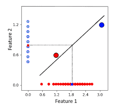
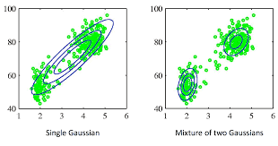
Clusters are groups of points that are similar to each other and dissimilar to points from other clusters. In terms of the underlying distribution, a cluster constitutes a connected area of high density around a mode of the distribution. Clusters may be determined automatically by clustering algorithms providing a flat clustering, or visually relying on the ability of human cognition to identify groups (see Gestalt laws of proximity and continuity detailed Sect. 1.3.2). Indeed, by looking at Fig. 1.7a, the reader gets an intuitive idea of what the clusters are for this dataset (a priori close to the automatic clustering of Fig. 1.8b).

Clustering algorithms identify a latent categorical variable indicating the cluster to which a given point belongs. Namely, they determine a mapping $\Omega: \mathcal{D} \longrightarrow \mathcal{L}$ assigning each data point $\xi_i$ to a category with a label $L_i=\Omega\left(\xi_i\right)$. The number of clusters, that is the number of possible values of that categorical variable, is a key parameter for a flat clustering. We may distinguish two main approaches for clustering of multidimensional data: the parametric approach used by partitioning algorithms and the density-based approach. For network data, the equivalent of clustering is community detection. In terms of graphs, communities (i.e. clusters) may be defined as groups of vertices linked together by many edges and linked to their surroundings by less edges [19].
Parametric Clustering
Partitioning algorithms, such as $k$-means [118] and $k$-medoids [96] split the space into $k$ convex regions parametrized by associated prototypes. Indeed, they assign each point of the datase to one of the clusters, so as to minimize the distances separating points from their clusters prototype. This prototype, which is respectively a centroid for $k$-means and a medoid for the $k$-medoids, provides a central tendency of the cluster. Formally, those algorithms seek the clustering that minimizes the cumulated Fréchet variance of all clusters, measured around their respective Fréchet means, which is the aforementioned prototype.

统计代写|数据结构作业代写data structure代考|Latent Variables Extraction and Manifold Learning

In the i.i.d hypothesis, the support of the theoretical probability distribution generating data points $\left{\xi_i\right}$ is considered as a manifold $\mathcal{M}$ immersed in the ambient data space $\mathcal{D}[9,81]$. The repartition of points along a manifold may be explained by the strong dependency between data space variables. In addition, one may assume that all these variables are local functions of a few independent latent variables with an additional noise [176], thus constituting a low-dimensional structure. That noise may induce small variations around the smooth structure of that manifold. Note that the manifold hypothesis may extend to datasets that are not generated by random processes. For instance, for the two open boxes and COIL-20 datasets (see Sect. 1.1.7), data lie on a low-dimensional manifold which is regularly sampled, and not randomly sampled.

Dimensionality Reduction (DR) in general aim at finding a mapping $\Phi: \mathcal{D} \longrightarrow$ $\mathcal{E}$, that associates each data point $\xi_i$ to a point $x_i=\Phi\left(\xi_i\right)$ in a low dimensional embedding space $\mathcal{E}$. A key parameter of dimensionality reduction is the embedding dimensionality $d$ (i.e. the dimensionality of $\mathcal{E}$ ). We distinguish here two sub-cases of $\mathrm{DK}$ : manifold learning and spatialization. The ideal goal of manifold learning is to extract latent variables parametrizing the manifold, which explain the variability of data. Those hypothetical variables may also be referred to as curvilinear components of the manifold [54]. In that case, the embedding dimensionality defines the number of variables to extract. A possible value for that parameter is the intrinsic dimensionality, which corresponds locally to the number of curvilinear components require to parametrize the manifold (see Sect. 2.2). Manifold learning may be used as a pre-processing step for other machine learning applications (e.g., classification or clustering), in order to mitigate the curse of dimensionality [155], to compress the data [179], or to filter out the noise [176]. Inversely, spatialization aims at providing a visual representation of high-dimensional data (see Sect. 1.3.2). As a result, the embedding dimensionality is constrained by the perceptual capabilities of the data analyst, limiting the number of dimensions to at most three for visualization with only one scatter plot. Satisfying this strong constraint on dimensionality often requires distortions of the underlying data structure. Note that the equivalent of DR for network data is graph embedding (also called graph layout).

数据结构代写

统计代写|数据结构作业代写data structure代考|Clusters and Flat Clustering

聚类是一组彼此相似但与其他聚类中的点不同的点。就底层分布而言，集群构成了围绕分布模式的高密度连接区域。聚类可以通过提供平面聚类的聚类算法自动确定，或者在视觉上依赖于人类认知能力来识别组（参见格式塔法则的邻近性和连续性详述第 1.3.2 节）。事实上，通过查看图 1.7a，读者可以直观地了解该数据集的聚类（先验接近图 1.8b 的自动聚类）。

聚类算法识别潜在分类变量，指示给定点所属的聚类。即，他们确定一个映射哦:丁⟶大号分配每个数据点X我到带有标签的类别大号我=哦(X我). 聚类的数量，即该分类变量的可能值的数量，是扁平聚类的关键参数。我们可以区分多维数据聚类的两种主要方法：分区算法使用的参数方法和基于密度的方法。对于网络数据，聚类相当于社区检测。在图方面，社区（即集群）可以定义为由许多边连接在一起并通过较少边连接到周围环境的顶点组 [19]。
参数聚类
分区算法，例如k-表示 [118] 和k-medoids [96] 将空间分割成k由相关原型参数化的凸区域。事实上，他们将数据集的每个点分配给其中一个集群，以最小化点与集群原型之间的距离。这个原型，分别是k-means 和 medoid 的k-medoids，提供集群的集中趋势。形式上，这些算法寻求最小化所有聚类的累积 Fréchet 方差的聚类，围绕它们各自的 Fréchet 均值测量，即上述原型。

统计代写|数据结构作业代写data structure代考|Latent Variables Extraction and Manifold Learning

在独立同分布假设下，生成数据点的理论概率分布的支持\左{\xi_i\右}\左{\xi_i\右}被认为是流形米沉浸在环境数据空间中丁[9,81]. 点沿流形的重新划分可以用数据空间变量之间的强依赖性来解释。此外，可以假设所有这些变量都是一些独立潜在变量的局部函数，带有额外的噪声[176]，从而构成一个低维结构。该噪声可能会在该流形的光滑结构周围引起微小的变化。请注意，流形假设可能会扩展到不是由随机过程生成的数据集。例如，对于两个开箱和 COIL-20 数据集（参见第 1.1.7 节），数据位于低维流形上，该流形是定期采样的，而不是随机采样的。

降维（DR）一般旨在寻找映射披:丁⟶ 和, 关联每个数据点X我到一点X我=披(X我)在低维嵌入空间和. 降维的一个关键参数是嵌入维数d（即维度和). 我们在这里区分两种子情况丁钾：流形学习和空间化。流形学习的理想目标是提取参数化流形的潜在变量，这解释了数据的可变性。这些假设变量也可以称为流形的曲线分量 [54]。在这种情况下，嵌入维度定义了要提取的变量数。该参数的一个可能值是固有维度，它局部对应于参数化流形所需的曲线分量的数量（参见第 2.2 节）。流形学习可用作其他机器学习应用程序（例如，分类或聚类）的预处理步骤，以减轻维数灾难 [155]、压缩数据 [179] 或滤除噪声[176]。反之，空间化旨在提供高维数据的可视化表示（参见第 1.3.2 节）。因此，嵌入维度受到数据分析师感知能力的限制，将维度的数量限制为最多三个，以便仅使用一个散点图进行可视化。满足这种对维度的强约束通常需要扭曲底层数据结构。请注意，网络数据的 DR 等效于图形嵌入（也称为图形布局）。满足这种对维度的强约束通常需要扭曲底层数据结构。请注意，网络数据的 DR 等效于图形嵌入（也称为图形布局）。满足这种对维度的强约束通常需要扭曲底层数据结构。请注意，网络数据的 DR 等效于图形嵌入（也称为图形布局）。

统计代写请认准statistics-lab™. statistics-lab™为您的留学生涯保驾护航。统计代写|python代写代考

随机过程代考

在概率论概念中，随机过程是随机变量的集合。 若一随机系统的样本点是随机函数，则称此函数为样本函数，这一随机系统全部样本函数的集合是一个随机过程。 实际应用中，样本函数的一般定义在时间域或者空间域。 随机过程的实例如股票和汇率的波动、语音信号、视频信号、体温的变化，随机运动如布朗运动、随机徘徊等等。

贝叶斯方法代考

贝叶斯统计概念及数据分析表示使用概率陈述回答有关未知参数的研究问题以及统计范式。后验分布包括关于参数的先验分布，和基于观测数据提供关于参数的信息似然模型。根据选择的先验分布和似然模型，后验分布可以解析或近似，例如，马尔科夫链蒙特卡罗 (MCMC) 方法之一。贝叶斯统计概念及数据分析使用后验分布来形成模型参数的各种摘要，包括点估计，如后验平均值、中位数、百分位数和称为可信区间的区间估计。此外，所有关于模型参数的统计检验都可以表示为基于估计后验分布的概率报表。

广义线性模型代考

广义线性模型（GLM）归属统计学领域，是一种应用灵活的线性回归模型。该模型允许因变量的偏差分布有除了正态分布之外的其它分布。

statistics-lab作为专业的留学生服务机构，多年来已为美国、英国、加拿大、澳洲等留学热门地的学生提供专业的学术服务，包括但不限于Essay代写，Assignment代写，Dissertation代写，Report代写，小组作业代写，Proposal代写，Paper代写，Presentation代写，计算机作业代写，论文修改和润色，网课代做，exam代考等等。写作范围涵盖高中，本科，研究生等海外留学全阶段，辐射金融，经济学，会计学，审计学，管理学等全球99%专业科目。写作团队既有专业英语母语作者，也有海外名校硕博留学生，每位写作老师都拥有过硬的语言能力，专业的学科背景和学术写作经验。我们承诺100%原创，100%专业，100%准时，100%满意。

机器学习代写

随着AI的大潮到来，Machine Learning逐渐成为一个新的学习热点。同时与传统CS相比，Machine Learning在其他领域也有着广泛的应用，因此这门学科成为不仅折磨CS专业同学的“小恶魔”，也是折磨生物、化学、统计等其他学科留学生的“大魔王”。学习Machine learning的一大绊脚石在于使用语言众多，跨学科范围广，所以学习起来尤其困难。但是不管你在学习Machine Learning时遇到任何难题，StudyGate专业导师团队都能为你轻松解决。

多元统计分析代考

基础数据: $N$ 个样本， $P$ 个变量数的单样本，组成的横列的数据表
变量定性: 分类和顺序；变量定量：数值
数学公式的角度分为: 因变量与自变量

时间序列分析代写

随机过程，是依赖于参数的一组随机变量的全体，参数通常是时间。 随机变量是随机现象的数量表现，其时间序列是一组按照时间发生先后顺序进行排列的数据点序列。通常一组时间序列的时间间隔为一恒定值（如1秒，5分钟，12小时，7天，1年），因此时间序列可以作为离散时间数据进行分析处理。研究时间序列数据的意义在于现实中，往往需要研究某个事物其随时间发展变化的规律。这就需要通过研究该事物过去发展的历史记录，以得到其自身发展的规律。

回归分析代写

多元回归分析渐进（Multiple Regression Analysis Asymptotics）属于计量经济学领域，主要是一种数学上的统计分析方法，可以分析复杂情况下各影响因素的数学关系，在自然科学、社会和经济学等多个领域内应用广泛。

MATLAB代写

MATLAB 是一种用于技术计算的高性能语言。它将计算、可视化和编程集成在一个易于使用的环境中，其中问题和解决方案以熟悉的数学符号表示。典型用途包括：数学和计算算法开发建模、仿真和原型制作数据分析、探索和可视化科学和工程图形应用程序开发，包括图形用户界面构建MATLAB 是一个交互式系统，其基本数据元素是一个不需要维度的数组。这使您可以解决许多技术计算问题，尤其是那些具有矩阵和向量公式的问题，而只需用 C 或 Fortran 等标量非交互式语言编写程序所需的时间的一小部分。MATLAB 名称代表矩阵实验室。MATLAB 最初的编写目的是提供对由 LINPACK 和 EISPACK 项目开发的矩阵软件的轻松访问，这两个项目共同代表了矩阵计算软件的最新技术。MATLAB 经过多年的发展，得到了许多用户的投入。在大学环境中，它是数学、工程和科学入门和高级课程的标准教学工具。在工业领域，MATLAB 是高效研究、开发和分析的首选工具。MATLAB 具有一系列称为工具箱的特定于应用程序的解决方案。对于大多数 MATLAB 用户来说非常重要，工具箱允许您学习和应用专业技术。工具箱是 MATLAB 函数（M 文件）的综合集合，可扩展 MATLAB 环境以解决特定类别的问题。可用工具箱的领域包括信号处理、控制系统、神经网络、模糊逻辑、小波、仿真等。

R语言代写	问卷设计与分析代写
PYTHON代写	回归分析与线性模型代写
MATLAB代写	方差分析与试验设计代写
STATA代写	机器学习/统计学习代写
SPSS代写	计量经济学代写
EVIEWS代写	时间序列分析代写
EXCEL代写	深度学习代写
SQL代写	各种数据建模与可视化代写

如果你也在 怎样代写数据结构data structure这个学科遇到相关的难题，请随时右上角联系我们的24/7代写客服。

数据结构是一种用于存储和组织数据的存储。它是一种在计算机上安排数据的方式，以便可以有效地访问和更新。根据你的要求和项目，为你的项目选择正确的数据结构很重要。

statistics-lab™ 为您的留学生涯保驾护航 在代写数据结构data structure方面已经树立了自己的口碑, 保证靠谱, 高质且原创的统计Statistics代写服务。我们的专家在代写数据结构data structure方面经验极为丰富，各种代写数据结构data structure相关的作业也就用不着说。

我们提供的数据结构data structure及其相关学科的代写，服务范围广, 其中包括但不限于:

• Statistical Inference 统计推断
• Statistical Computing 统计计算
• Advanced Probability Theory 高等楖率论
• Advanced Mathematical Statistics 高等数理统计学
• (Generalized) Linear Models 广义线性模型
• Statistical Machine Learning 统计机器学习
• Longitudinal Data Analysis 纵向数据分析
• Foundations of Data Science 数据科学基础

统计代写|数据结构作业代写data structure代考|Multidimensional Data

Multidimensional data (also called feature data or tabular data) correspond to a set of $N$ data points (or feature vectors) $\xi_i$ in a high dimensional vector space $\mathcal{D}$. This data space (or feature space) $\mathcal{D}$ of dimensionality $\delta$ often corresponds to $\mathbb{R}^\delta$. A multidimensional dataset may be stored in a data matrix $\Xi$ of size $N \times \delta$. The element $(i, k)$ of that matrix, denoted $\xi_{i k}$, contains the value of the $k$ th variable for the $i$ th data point $\xi_i$.

Multidimensional data is thus the natural format for treating data tables, which are the basic element of relational databases (e.g., SQL databases). Indeed, those tables are organized by rows and columns, each row corresponding to an instance, and each column being associated with an attribute (or feature) of that instance. In statistics, those instances are also called individuals or observations.

The features are either quantitative, such as numerical or ordinal variables, or qualitative, as for categorical or boolean variables. Yet, all these types of variables may be stored in a common numerical matrix with, for example, ordinal variables represented by successive integers, boolean variables by 0 and 1 values and categorical variables represented by several boolean variables (one by category), each indicating whether the observation belongs to that category [179].

For a data matrix $\boldsymbol{\Xi}$, an associated distance matrix $\boldsymbol{\Delta} \boldsymbol{\Xi}$ may be obtained by choosing a specific metric $\Delta$ on the data space. Dimensionality reduction seeks to convert metric data into multidimensional data in a low dimensional space, thus leading to a set of $N$ embedded points $x_i$ in a low dimensional embedding space $\mathcal{E}$ of dimensionality $d$.

统计代写|数据结构作业代写data structure代考|Network Data

Networks data characterize relations between instances, as can be stored in a relation table in relational databases. As such, they can be modelled by a graph (as formally defined by Definition 1.4). They may either be hierarchical data (tree structures) or relational data (graph structures).

Definition 1.4 A weighted directed graph (or digraph) $G=(V, E, W)$ is composed of:

• $V$ the set of $N$ vertices,
• $E \subseteq V \times V$ the set of directed edges with cardinal $|E| \leqslant N^2$,
• $W$ the set of weights associated to the edges.
  The vertices $i \in V$ of that graph correspond to instances and edges $(i, j) \in E$ to the relations existing between the instances $i$ and $j$. The associated weights $w_{i j}$ characterize those relations. They may, for example, be measures of similarity $\gamma_{i j}$ or measures of dissimilarity $\Delta_{i j}$. A graph weighted by similarities may be represented by its adjacency matrix whose element $(i, j)$ contains the weight $w_{i j}$ if the edge $(i, j)$ exists and 0 otherwise. For non-complete graph, that matrix is sparse. This representation could be adapted to graphs weighted by dissimilarities by denoting non-existing edges with elements equal to $+\infty$.
  Graph Distances
  Weights of a graph often define similarities or dissimilarities between some pairs of vertices. Graph distances rely on this sparse information to define a full distance matrix $\Delta$ measuring dissimilarity between all pairs of vertices.

Shortest path distances [175] find the path of minimum length between two vertices in the graph weighted by dissimilarities. Conversely, in graphs weighted by similarities, distances tend to rely on random walks. Those random walks take a random path resulting from successive random transitions, where the probability of transitioning from a vertex $i$ to any other vertex $j$ is proportional to the weight $w_{i j}$.

数据结构代写

统计代写|数据结构作业代写data structure代考|Multidimensional Data

多维数据 (也称为特征数据或表格数据) 对应于一组 $N$ 数据点 (或特征向量) $\xi_i$ 在高维向量空 间 D. 这个数据空间 (或特征空间) $\mathcal{D}$ 维度的 $\delta$ 通常对应于䄳 . 多维数据集可以存储在数据矩阵
因此，多维数据是处理数据表的自然格式，而数据表是关系数据库 (例如，SQL 数据库) 的基 本元素。事实上，这些表是按行和列组织的，每一行对应一个实例，每一列与该实例的一个属 性（或特征) 相关联。在统计学中，这些实例也称为个体或观察值。
这些特征要么是定量的，例如数值或有序变量，要么是定性的，例如分类或布尔变量。然而， 所有这些类型的变量都可以存储在一个公共数值矩阵中，例如，序数变量由连续的整数表示， 布尔变量由 0 和 1 值表示，分类变量由几个布尔变量 (一个按类别) 表示，每个表示观察是否 属于该类别[179]。
对于数据矩阵 $\Xi$,一个相关的距离矩阵 $\Delta \Xi$ 可以通过选择特定指标获得 $\Delta$ 在数据空间上。降维 寻求将度量数据转换为低维空间中的多维数据，从而导致一组 $N$ 嵌入点 $x_i$ 在低维嵌入空间 $\mathcal{E}$ 维 度的 $d$.

统计代写|数据结构作业代写data structure代考|Network Data

网络数据表征实例之间的关系，可以存储在关系数据库的关系表中。因此，它们可以用图来建 模 (如定义 $1.4$ 中正式定义的那样）。它们可以是分层数据（树结构) 或关系数据（图形结 构) 。
定义 $1.4$ 加权有向图 (或有向图) $G=(V, E, W)$ 由…组成:

• $V$ 的集合 $N$ 顶点，
• $E \subseteq V \times V$ 有基数的有向边集 $|E| \leqslant N^2$,
• $W$ 与边关联的一组权重。
  顶点 $i \in V$ 该图对应于实例和边缘 $(i, j) \in E$ 实例之间存在的关系 $i$ 和 $j$. 相关权重 $w_{i j}$ 表征 这些关系。例如，它们可能是相似性的度量 $\gamma_{i j}$ 或不同的措施 $\Delta_{i j}$. 由相似性加权的图可以 由其元素的邻接矩阵表示 $(i, j)$ 包含重量 $w_{i j}$ 如果边缘 $(i, j)$ 存在，否则为 0 。对于非完全 图，该矩阵是稀疏的。这种表示可以通过用等于 $+\infty$.
  图形距离图形
  的权重通常定义某些顶点对之间的相似性或不同性。图距离依赖于这种稀疏信息来定义一 个完整的距离矩阵 $\Delta$ 测量所有顶点对之间的差异性。
  最短路径距离 [175] 找到图中两个顶点之间由差异加权的最小长度路径。相反，在由相似性加 权的图中，距离往往依赖于随机游走。这些随机斿走采用由连续随机转换产生的随机路径，其 中从顶点转换的概率 $i$ 到任何其他顶点 $j$ 与重量成正比 $w_{i j}$.

统计代写请认准statistics-lab™. statistics-lab™为您的留学生涯保驾护航。统计代写|python代写代考

随机过程代考

在概率论概念中，随机过程是随机变量的集合。 若一随机系统的样本点是随机函数，则称此函数为样本函数，这一随机系统全部样本函数的集合是一个随机过程。 实际应用中，样本函数的一般定义在时间域或者空间域。 随机过程的实例如股票和汇率的波动、语音信号、视频信号、体温的变化，随机运动如布朗运动、随机徘徊等等。

贝叶斯方法代考

贝叶斯统计概念及数据分析表示使用概率陈述回答有关未知参数的研究问题以及统计范式。后验分布包括关于参数的先验分布，和基于观测数据提供关于参数的信息似然模型。根据选择的先验分布和似然模型，后验分布可以解析或近似，例如，马尔科夫链蒙特卡罗 (MCMC) 方法之一。贝叶斯统计概念及数据分析使用后验分布来形成模型参数的各种摘要，包括点估计，如后验平均值、中位数、百分位数和称为可信区间的区间估计。此外，所有关于模型参数的统计检验都可以表示为基于估计后验分布的概率报表。

广义线性模型代考

广义线性模型（GLM）归属统计学领域，是一种应用灵活的线性回归模型。该模型允许因变量的偏差分布有除了正态分布之外的其它分布。

statistics-lab作为专业的留学生服务机构，多年来已为美国、英国、加拿大、澳洲等留学热门地的学生提供专业的学术服务，包括但不限于Essay代写，Assignment代写，Dissertation代写，Report代写，小组作业代写，Proposal代写，Paper代写，Presentation代写，计算机作业代写，论文修改和润色，网课代做，exam代考等等。写作范围涵盖高中，本科，研究生等海外留学全阶段，辐射金融，经济学，会计学，审计学，管理学等全球99%专业科目。写作团队既有专业英语母语作者，也有海外名校硕博留学生，每位写作老师都拥有过硬的语言能力，专业的学科背景和学术写作经验。我们承诺100%原创，100%专业，100%准时，100%满意。

机器学习代写

随着AI的大潮到来，Machine Learning逐渐成为一个新的学习热点。同时与传统CS相比，Machine Learning在其他领域也有着广泛的应用，因此这门学科成为不仅折磨CS专业同学的“小恶魔”，也是折磨生物、化学、统计等其他学科留学生的“大魔王”。学习Machine learning的一大绊脚石在于使用语言众多，跨学科范围广，所以学习起来尤其困难。但是不管你在学习Machine Learning时遇到任何难题，StudyGate专业导师团队都能为你轻松解决。

多元统计分析代考

基础数据: $N$ 个样本， $P$ 个变量数的单样本，组成的横列的数据表
变量定性: 分类和顺序；变量定量：数值
数学公式的角度分为: 因变量与自变量

时间序列分析代写

随机过程，是依赖于参数的一组随机变量的全体，参数通常是时间。 随机变量是随机现象的数量表现，其时间序列是一组按照时间发生先后顺序进行排列的数据点序列。通常一组时间序列的时间间隔为一恒定值（如1秒，5分钟，12小时，7天，1年），因此时间序列可以作为离散时间数据进行分析处理。研究时间序列数据的意义在于现实中，往往需要研究某个事物其随时间发展变化的规律。这就需要通过研究该事物过去发展的历史记录，以得到其自身发展的规律。

回归分析代写

多元回归分析渐进（Multiple Regression Analysis Asymptotics）属于计量经济学领域，主要是一种数学上的统计分析方法，可以分析复杂情况下各影响因素的数学关系，在自然科学、社会和经济学等多个领域内应用广泛。

MATLAB代写

MATLAB 是一种用于技术计算的高性能语言。它将计算、可视化和编程集成在一个易于使用的环境中，其中问题和解决方案以熟悉的数学符号表示。典型用途包括：数学和计算算法开发建模、仿真和原型制作数据分析、探索和可视化科学和工程图形应用程序开发，包括图形用户界面构建MATLAB 是一个交互式系统，其基本数据元素是一个不需要维度的数组。这使您可以解决许多技术计算问题，尤其是那些具有矩阵和向量公式的问题，而只需用 C 或 Fortran 等标量非交互式语言编写程序所需的时间的一小部分。MATLAB 名称代表矩阵实验室。MATLAB 最初的编写目的是提供对由 LINPACK 和 EISPACK 项目开发的矩阵软件的轻松访问，这两个项目共同代表了矩阵计算软件的最新技术。MATLAB 经过多年的发展，得到了许多用户的投入。在大学环境中，它是数学、工程和科学入门和高级课程的标准教学工具。在工业领域，MATLAB 是高效研究、开发和分析的首选工具。MATLAB 具有一系列称为工具箱的特定于应用程序的解决方案。对于大多数 MATLAB 用户来说非常重要，工具箱允许您学习和应用专业技术。工具箱是 MATLAB 函数（M 文件）的综合集合，可扩展 MATLAB 环境以解决特定类别的问题。可用工具箱的领域包括信号处理、控制系统、神经网络、模糊逻辑、小波、仿真等。

R语言代写	问卷设计与分析代写
PYTHON代写	回归分析与线性模型代写
MATLAB代写	方差分析与试验设计代写
STATA代写	机器学习/统计学习代写
SPSS代写	计量经济学代写
EVIEWS代写	时间序列分析代写
EXCEL代写	深度学习代写
SQL代写	各种数据建模与可视化代写

如果你也在 怎样代写数据结构data structure这个学科遇到相关的难题，请随时右上角联系我们的24/7代写客服。

数据结构是一种用于存储和组织数据的存储。它是一种在计算机上安排数据的方式，以便可以有效地访问和更新。根据你的要求和项目，为你的项目选择正确的数据结构很重要。

statistics-lab™ 为您的留学生涯保驾护航 在代写数据结构data structure方面已经树立了自己的口碑, 保证靠谱, 高质且原创的统计Statistics代写服务。我们的专家在代写数据结构data structure方面经验极为丰富，各种代写数据结构data structure相关的作业也就用不着说。

我们提供的数据结构data structure及其相关学科的代写，服务范围广, 其中包括但不限于:

• Statistical Inference 统计推断
• Statistical Computing 统计计算
• Advanced Probability Theory 高等楖率论
• Advanced Mathematical Statistics 高等数理统计学
• (Generalized) Linear Models 广义线性模型
• Statistical Machine Learning 统计机器学习
• Longitudinal Data Analysis 纵向数据分析
• Foundations of Data Science 数据科学基础

统计代写|数据结构作业代写data structure代考|Measuring Dissimilarities and Similarities

Data instances of any type may be considered as points in a metric space as long as one may define a metric or distance function to measure the dissimilarity between two instances. This metric space $(\mathcal{D}, \Delta)$ is a topological space equipped with a distance $\Delta$, which provides for each pair of elements of that space a numerical score of their dissimilarity. This proper notion of distance is defined by:

Definition 1.1 A function $\Delta: \mathcal{D} \times \mathcal{D} \rightarrow \mathbb{R}^{+}$is a distance (or metric) over the space $\mathcal{D}$ if and only if it satisfies the following conditions for all $\xi_i, \xi_j, \xi_k \in \mathcal{D}$ :

• $\Delta\left(\xi_i, \xi_j\right) \geqslant 0$ (non-negativity),
• $\Delta\left(\xi_i, \xi_j\right)=0$ iff $\xi_i=\xi_j$ (identity of indiscernibles),
• $\Delta\left(\xi_i, \xi_j\right)=\Delta\left(\xi_j, \xi_i\right)$ (symmetry)
• $\Delta\left(\xi_l, \xi_j\right) \leqslant \Delta\left(\xi_l, \xi_k\right)+\Delta\left(\xi_k, \xi_j\right)$ (triangle inequality or sub-additivity).
  Those distances extend to abstract spaces the spatial notion of distance in our three-dimensional physical space, measured using the Euclidean distance (see Sect. 1.1.4). As a tool for measuring dissimilarities, one may also consider pseudometrics which do not satisfy all properties of the Definition 1.1. When not otherwise stated dissimilarities between data are computed with the Euclidean distance.

Metric spaces are a more general case of normed vector spaces, that is spaces equipped with a norm $|\cdot|$ measuring the size of a vector, defined as follows:

Definition 1.2 A function $|\cdot|: \mathcal{D} \longrightarrow \mathbb{R}^{+}$is a norm if and only if it satisfies the properties for all $\xi_i, \xi_j \in \mathcal{D}$ and $\alpha \in \mathbb{R}$ :

• $\left|\alpha \xi_i\right|=|\alpha|\left|\xi_i\right|$ (homogeneity),
• $\left|\xi_i\right|=0 \Rightarrow \xi_i=0$ (separation),
• $\left|\xi_i+\xi_j\right| \leqslant\left|\xi_i\right|+\left|\xi_j\right|$ (triangle inequality).
  In a normed vector space, a distance is naturally defined between all pairs of point by computing the norm of their difference:
  $$
  \Delta\left(\xi_i, \xi_j\right)=\left|\xi_i-\xi_j\right| .
  $$
  Normed vector spaces include the subcase of inner product spaces (equipped with an inner product $\langle\cdot, \cdot\rangle$. An inner product must satisfy the following definition.

统计代写|数据结构作业代写data structure代考|Neighbourhood Ranks

Neighbourhood ranks reduce the information of distances for a given dataset to an ordering, considering independently each row of the distance matrix. The rank $\rho_{i j}$ describes the position of point $\xi_j$ in the neighbourhood of point $\xi_i$, that is its place in the sorting of data points by their distance to point $\xi_i$. Replacing distances values by their ranks ensures more robustness to the phenomenon of norm concentration detailed in Sect. 2.1. Formally, a rank $\rho_{i j}$ indicates that point $\xi_j$ is the $\rho_{i j}$ th nearest neighbour of point $\xi_i$. By convention, we set $\rho_{i i} \triangleq 0$.

For each data point $\xi_i$, we define the neighbourhood permutation $\tilde{v}i: \llbracket 0, N-1 \rrbracket \longrightarrow \llbracket 1 ; N \rrbracket$ as the mapping returning for a given rank $\kappa$, the index $j$ of the $\kappa$ th nearest neighbour of $\xi_i$ in that space. Namely, $\tilde{v}_i(\kappa)$ is the index so that $\xi{\tilde{v}i(\kappa)}$ is the $\kappa$ th nearest neighbour of $\xi_i$. We may note that $\tilde{v}_i\left(\rho{i j}\right)=j$ and that, using the bijectivity of the permutation, $\rho_{i j}=\tilde{v}_i^{-1}(j)$ (which may be an alternative definition of ranks).

We also define $\kappa$-neighbourhoods $v_i(\kappa)$ as the set of indices of the $\kappa$ nearest neighbours of $i$. This may be formally defined based on ranks as $v_i(\kappa)={j \neq i \mid$ $\left.\rho_{i j} \leqslant \kappa\right}$, or as the image by the neighbourhood permutation $\tilde{v}_i$ of the set $\llbracket 1 ; \kappa \rrbracket$, namely $v_i(\kappa)=\tilde{v}_i(\llbracket 1 ; \kappa \rrbracket)$. The link between distances, neighbourhood ranks and neighbourhood permutations is illustrated Fig. 1.1, for an abstract metric dataset.

数据结构代写

统计代写|数据结构作业代写data structure代考|Measuring Dissimilarities and Similarities

任何类型的数据实例都可以被视为度量空间中的点，只要可以定义度量或距离函数来衡量两个 实例之间的差异即可。这个度量空间 $(\mathcal{D}, \Delta)$ 是一个带有距离的拓扑空间 $\Delta$ ，它为该空间的每对 元素提供了它们相异性的数值分数。这个距离的正确概念定义为:
定义 $1.1$ 函数 $\Delta: \mathcal{D} \times \mathcal{D} \rightarrow \mathbb{R}^{+}$是空间上的距离 (或度量) $\mathcal{D}$ 当且仅当它满足以下所有条件 $\xi_i, \xi_j, \xi_k \in \mathcal{D}$ :

• $\Delta\left(\xi_i, \xi_j\right) \geqslant 0$ (非负性)，
• $\Delta\left(\xi_i, \xi_j\right)=0$ 当且仅当 $\xi_i=\xi_j$ (不可辨认者的身份），
• $\Delta\left(\xi_i, \xi_j\right)=\Delta\left(\xi_j, \xi_i\right)$ (对称)
• $\Delta\left(\xi_l, \xi_j\right) \leqslant \Delta\left(\xi_l, \xi_k\right)+\Delta\left(\xi_k, \xi_j\right)$ (三角不等式或子可加性) 。
  这些距离将我们的三维物理空间中距离的空间概念扩展到抽象空间，使用欧几里德距离测 量 (参见第 1.1.4 节) 。作为一种测量差异的工具，人们还可以考虑不满足定义 $1.1$ 的所 有属性的伪度量。如果没有另外说明，数据之间的差异是用欧氏距离计算的。
  度量空间是赋范向量空间的更一般情况，即配备范数的空间 |·|测量向量的大小，定义如下:
  定义 $1.2$ 函数 $|\cdot|: \mathcal{D} \longrightarrow \mathbb{R}^{+}$是一个规范当且仅当它满足所有的属性 $\xi_i, \xi_j \in \mathcal{D}$ 和 $\alpha \in \mathbb{R}$ :
• $\left|\alpha \xi_i\right|=|\alpha|\left|\xi_i\right|$ (同质性)，
• $\left|\xi_i\right|=0 \Rightarrow \xi_i=0$ (分离) ，
• $\left|\xi_i+\xi_j\right| \leqslant\left|\xi_i\right|+\left|\xi_j\right|$ (三角不等式) 。 在陚范向量空间中，通过计算点对差的范数自然地定义了所有点对之间的距离:
  $$
  \Delta\left(\xi_i, \xi_j\right)=\left|\xi_i-\xi_j\right| .
  $$
  赋范向量空间包括内积空间的子情况 (配备内积 $\langle\cdot, \cdot\rangle$. 内积必须满足以下定义。

统计代写|数据结构作业代写data structure代考|Neighbourhood Ranks

邻域等级将给定数据集的距离信息减少为排序，独立考虑距离矩阵的每一行。排名 $\rho_{i j}$ 描述点的 位置 $\xi_j$ 在点附近 $\xi_i$ ，这是它在按点到点的距离对数据点进行排序时的位置 $\xi_i$. 用等级替换距离值 可确保对第 1 节中详述的范数集中现象具有更强的鲁棒性。2.1. 正式地，等级 $\rho_{i j}$ 表示那一点 $\xi_j$ 是个 $\rho_{i j}$ 点的第 th 个最近邻点 $\xi_i$. 按昭惯例，我们设 $\rho_{i i} \triangleq 0$.
对于每个数据点 $\xi_i$ ，我们定义邻域置换
$\tilde{v} i: \backslash$ llbracket $0, N-1 \backslash$ rrbracket $\longrightarrow \backslash$ llbracket $1 ; N \backslash$ rrbracket作为给定等级的 $\kappa$ 的第 th 个最近邻 $\xi_i$. 我们可能注意到 $\tilde{v}i(\rho i j)=j$ 并且，使用排列的双射性， $\rho{i j}=\tilde{v}i^{-1}(j)$ (这可能是等级的另一种定义) 。 我们还定义 $\kappa$-社区 $v_i(\kappa)$ 作为指数的集合 $\kappa$ 最近的邻居 $i$. 这可以根据等级正式定义为 V_i(lkappa)={j Ineq i mid\$ \$Vleft.Irho{i j} leqslant Ikappalright}}，或者作为邻域非列的图像 $\tilde{v}_i$ 集 合的 $\backslash$ llbracket $1 ; \kappa \backslash$ rrbracket, 即 $v_i(\kappa)=\tilde{v}_i(\backslash$ llbracket $1 ; \kappa \backslash$ rrbracket). 对于抽象度 量数据集，距离、邻域等级和邻域排列之间的联系如图 $1.1$ 所示。

统计代写请认准statistics-lab™. statistics-lab™为您的留学生涯保驾护航。统计代写|python代写代考

随机过程代考

在概率论概念中，随机过程是随机变量的集合。 若一随机系统的样本点是随机函数，则称此函数为样本函数，这一随机系统全部样本函数的集合是一个随机过程。 实际应用中，样本函数的一般定义在时间域或者空间域。 随机过程的实例如股票和汇率的波动、语音信号、视频信号、体温的变化，随机运动如布朗运动、随机徘徊等等。

贝叶斯方法代考

贝叶斯统计概念及数据分析表示使用概率陈述回答有关未知参数的研究问题以及统计范式。后验分布包括关于参数的先验分布，和基于观测数据提供关于参数的信息似然模型。根据选择的先验分布和似然模型，后验分布可以解析或近似，例如，马尔科夫链蒙特卡罗 (MCMC) 方法之一。贝叶斯统计概念及数据分析使用后验分布来形成模型参数的各种摘要，包括点估计，如后验平均值、中位数、百分位数和称为可信区间的区间估计。此外，所有关于模型参数的统计检验都可以表示为基于估计后验分布的概率报表。

广义线性模型代考

广义线性模型（GLM）归属统计学领域，是一种应用灵活的线性回归模型。该模型允许因变量的偏差分布有除了正态分布之外的其它分布。

statistics-lab作为专业的留学生服务机构，多年来已为美国、英国、加拿大、澳洲等留学热门地的学生提供专业的学术服务，包括但不限于Essay代写，Assignment代写，Dissertation代写，Report代写，小组作业代写，Proposal代写，Paper代写，Presentation代写，计算机作业代写，论文修改和润色，网课代做，exam代考等等。写作范围涵盖高中，本科，研究生等海外留学全阶段，辐射金融，经济学，会计学，审计学，管理学等全球99%专业科目。写作团队既有专业英语母语作者，也有海外名校硕博留学生，每位写作老师都拥有过硬的语言能力，专业的学科背景和学术写作经验。我们承诺100%原创，100%专业，100%准时，100%满意。

机器学习代写

随着AI的大潮到来，Machine Learning逐渐成为一个新的学习热点。同时与传统CS相比，Machine Learning在其他领域也有着广泛的应用，因此这门学科成为不仅折磨CS专业同学的“小恶魔”，也是折磨生物、化学、统计等其他学科留学生的“大魔王”。学习Machine learning的一大绊脚石在于使用语言众多，跨学科范围广，所以学习起来尤其困难。但是不管你在学习Machine Learning时遇到任何难题，StudyGate专业导师团队都能为你轻松解决。

多元统计分析代考

基础数据: $N$ 个样本， $P$ 个变量数的单样本，组成的横列的数据表
变量定性: 分类和顺序；变量定量：数值
数学公式的角度分为: 因变量与自变量

时间序列分析代写

随机过程，是依赖于参数的一组随机变量的全体，参数通常是时间。 随机变量是随机现象的数量表现，其时间序列是一组按照时间发生先后顺序进行排列的数据点序列。通常一组时间序列的时间间隔为一恒定值（如1秒，5分钟，12小时，7天，1年），因此时间序列可以作为离散时间数据进行分析处理。研究时间序列数据的意义在于现实中，往往需要研究某个事物其随时间发展变化的规律。这就需要通过研究该事物过去发展的历史记录，以得到其自身发展的规律。

回归分析代写

多元回归分析渐进（Multiple Regression Analysis Asymptotics）属于计量经济学领域，主要是一种数学上的统计分析方法，可以分析复杂情况下各影响因素的数学关系，在自然科学、社会和经济学等多个领域内应用广泛。

MATLAB代写

MATLAB 是一种用于技术计算的高性能语言。它将计算、可视化和编程集成在一个易于使用的环境中，其中问题和解决方案以熟悉的数学符号表示。典型用途包括：数学和计算算法开发建模、仿真和原型制作数据分析、探索和可视化科学和工程图形应用程序开发，包括图形用户界面构建MATLAB 是一个交互式系统，其基本数据元素是一个不需要维度的数组。这使您可以解决许多技术计算问题，尤其是那些具有矩阵和向量公式的问题，而只需用 C 或 Fortran 等标量非交互式语言编写程序所需的时间的一小部分。MATLAB 名称代表矩阵实验室。MATLAB 最初的编写目的是提供对由 LINPACK 和 EISPACK 项目开发的矩阵软件的轻松访问，这两个项目共同代表了矩阵计算软件的最新技术。MATLAB 经过多年的发展，得到了许多用户的投入。在大学环境中，它是数学、工程和科学入门和高级课程的标准教学工具。在工业领域，MATLAB 是高效研究、开发和分析的首选工具。MATLAB 具有一系列称为工具箱的特定于应用程序的解决方案。对于大多数 MATLAB 用户来说非常重要，工具箱允许您学习和应用专业技术。工具箱是 MATLAB 函数（M 文件）的综合集合，可扩展 MATLAB 环境以解决特定类别的问题。可用工具箱的领域包括信号处理、控制系统、神经网络、模糊逻辑、小波、仿真等。

R语言代写	问卷设计与分析代写
PYTHON代写	回归分析与线性模型代写
MATLAB代写	方差分析与试验设计代写
STATA代写	机器学习/统计学习代写
SPSS代写	计量经济学代写
EVIEWS代写	时间序列分析代写
EXCEL代写	深度学习代写
SQL代写	各种数据建模与可视化代写