标签: CSAT3350

电子工程代写|三维成像代写Three-Dimensional Imaging代考|EE262

如果你也在 怎样代写三维成像Three-Dimensional Imaging这个学科遇到相关的难题,请随时右上角联系我们的24/7代写客服。

三维成像是一种将许多扫描(来自计算机断层扫描、核磁共振或超声扫描)通过计算结合起来的技术。然后,这些图像可以由放射科医师或医生进行操作,以帮助诊断和手术计划。

statistics-lab™ 为您的留学生涯保驾护航 在代写三维成像Three-Dimensional Imaging方面已经树立了自己的口碑, 保证靠谱, 高质且原创的统计Statistics代写服务。我们的专家在代写三维成像Three-Dimensional Imaging方面经验极为丰富,各种代写三维成像Three-Dimensional Imaging相关的作业也就用不着说。

我们提供的三维成像Three-Dimensional Imaging及其相关学科的代写,服务范围广, 其中包括但不限于:

  • Statistical Inference 统计推断
  • Statistical Computing 统计计算
  • Advanced Probability Theory 高等楖率论
  • Advanced Mathematical Statistics 高等数理统计学
  • (Generalized) Linear Models 广义线性模型
  • Statistical Machine Learning 统计机器学习
  • Longitudinal Data Analysis 纵向数据分析
  • Foundations of Data Science 数据科学基础
电子工程代写|三维成像代写Three-Dimensional Imaging代考|EE262

电子工程代写|三维成像代写Three-Dimensional Imaging代考|Effect of Pixel Pitch

Here, it is assumed the elemental image has a pixel structure, and the pitch is given by $P_{N P}$. The elemental image is sampled by the pixels on the elemental images. The maximum projected spatial frequency of the object is limited by the Nyquist frequency:
$$
\alpha_{N P} \cong \frac{g}{2 P_{N P}} .
$$
Visual spatial frequency $\beta_{N P}$ according to $\alpha_{\mathrm{NP}}$, is given by Eq. (1.39):
$$
\beta_{N P}=\alpha_{N P} \frac{L_{O B}-Z_{s}}{\left|Z_{s}\right|}=\frac{g}{2 P_{N P}} \frac{L_{O B}-Z_{s}}{\left|Z_{s}\right|}
$$
Here, assuming $-z_{s}$ is infinite, we obtain:
$$
\beta_{N P}=\frac{g}{2 P_{N P}} .
$$
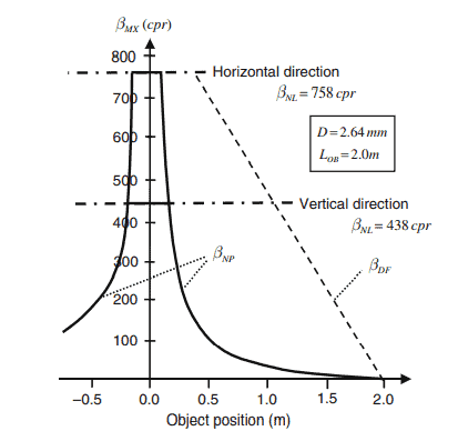
Maximum visual spatial frequency $\beta_{M X}$ is given by the following equation:
$$
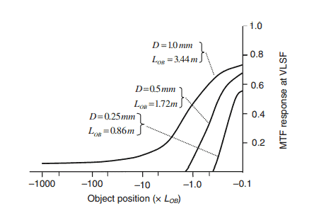
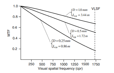
\boldsymbol{\beta}{M X}=\min \left(\boldsymbol{\beta}{N P}, \boldsymbol{\beta}{D F}, \boldsymbol{\beta}{V L}, \boldsymbol{\beta}{N L}\right) $$ where $\beta{D F}$ is a spatial frequency that gives the null response by diffraction or the defocus described in the former section. When the diameter of the elemental lens is more than about $1.0 \mathrm{~mm}, \beta_{D F}$ is more than $\beta_{V L}$ under the condition in Eq. (1.42). If the pixel pitch of each elemental image $P_{N P}$ is too large, the MTF response depends mainly on the Nyquist frequency $\beta_{N P}$ by the pixel pitch.
The viewing zone is given by [19]
$$
\boldsymbol{\phi}{V Z} \cong \frac{P{a}}{g}
$$
A wide viewing zone requires small $\mathrm{g}$, but small $g$ degrades $\beta_{N P}$. To compensate for the degradation, $P_{N P}$ needs to be smaller.

电子工程代写|三维成像代写Three-Dimensional Imaging代考|Experimental System

To obtain moving pictures, an electronic capture device, such as a CCD or CMOS image sensor, is set on the capture plate and takes elemental images. For reconstruction, a display device such as an LCD panel or an EL panel is placed behind the lens array. Video signals are transmitted from the capture device to the display device.

The size of the lens array for capturing needs to be large enough to obtain a large parallax; however, it is difficult to develop a large capture device for moving pictures. In the actual system, a television camera using a pickup lens is set to capture all elemental images formed by the elemental lenses. In the future, a capture device of the same size as the lens array will need to be developed and set immediately behind the lens array.

Figure $1.6$ shows an experimental real-time integral imaging system. A depth control lens, a GRIN lens array [14, 15], a converging lens, and an EHR (extremely high resolution) camera with 2,000 scanning lines [23] are introduced for capturing. The depth control lens [10] forms the optical image of the object around the lens array, and the GRIN lens array captures the optical image. Many elemental lenses (GRIN lenses) form elemental images near the output plane of the array. An elemental GRIN lens acts as a specific lens forming an erect image for the object in the distant R.O. area to avoid pseudoscopic 3-D images. The converging lens [10], which is set close to the GRIN lens array, leads the light rays from elemental GRIN lenses to the EHR camera. The converging lens uses light rays efficiently, but is not an essential which are formed around the output plane of the GRIN lens.

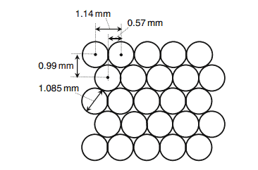
Table $1.1$ shows the experimental specifications of the capture setup. Figure $1.7$ shows the two-dimensional arrangement of the GRIN lens array used in the experiment. The pitch between the adjacent elemental lenses corresponds to $21.3$ pixels of the EHR camera. The arrangement has a delta structure, which is more efficient than a grid structure. The horizontal pitch is considered $21.3 / 2$ and the vertical one is considered $21.3 \times \sqrt{3} / 2$, equivalently.

电子工程代写|三维成像代写Three-Dimensional Imaging代考|EE262

三维成像代考

电子工程代写|三维成像代写Three-Dimensional Imaging代考|Effect of Pixel Pitch

这里,假设元素图像具有像素结构,并且间距由下式给出 $P_{N P}$. 元素图像由元素图像上的像素采样。物体的最大投 影空间频率受奈奎斯特频率的限制:
$$
\alpha_{N P} \cong \frac{g}{2 P_{N P}}
$$
视觉空间频率 $\beta_{N P}$ 根据 $\alpha_{\mathrm{NP}}$, 由等式给出。(1.39):
$$
\beta_{N P}=\alpha_{N P} \frac{L_{O B}-Z_{s}}{\left|Z_{s}\right|}=\frac{g}{2 P_{N P}} \frac{L_{O B}-Z_{s}}{\left|Z_{s}\right|}
$$
在这里,假设 $-z_{s}$ 是无限的,我们得到:
$$
\beta_{N P}=\frac{g}{2 P_{N P}} .
$$
最大视觉空间频率 $\beta_{M X}$ 由以下等式给出:
$$
\boldsymbol{\beta} M X=\min (\boldsymbol{\beta} N P, \boldsymbol{\beta} D F, \boldsymbol{\beta} V L, \boldsymbol{\beta} N L)
$$
在哪里 $\beta D F$ 是一个空间频率,它通过前一节中描述的衍射或散焦给出零响应。当元素透镜的直径大于约 $1.0 \mathrm{~mm}, \beta_{D F}$ 超过 $\beta_{V L}$ 在方程式中的条件下。(1.42)。如果每个元素图像的像素间距 $P_{N P}$ 太大,MTF响应主要取 决于奈奎斯特频率 $\beta_{N P}$ 通过像素间距。 视域由 [19] 给出
$$
\phi V Z \cong \frac{P a}{g}
$$
宽视区需要小 $\mathrm{g}$, 但很小 $g$ 降级 $\beta_{N P}$. 为了弥补退化, $P_{N P}$ 需要更小。

电子工程代写|三维成像代写Three-Dimensional Imaging代考|Experimental System

为了获得运动图像,电子捕捉设备,例如CCD或CMOS图像传感器,被设置在捕捉板上并拍摄元素图像。为了重建,将诸如 LCD 面板或 EL 面板之类的显示设备放置在透镜阵列的后面。视频信号从捕获设备传输到显示设备。

用于捕捉的透镜阵列的尺寸需要足够大,以获得较大的视差;然而,很难开发用于运动图像的大型捕捉设备。在实际系统中,使用拾取镜头的电视摄像机被设置为捕获由元素镜头形成的所有元素图像。未来,需要开发与镜头阵列大小相同的捕捉设备,并将其设置在镜头阵列的正后方。

数字1.6显示了一个实验性的实时积分成像系统。引入了深度控制透镜、GRIN 透镜阵列 [14、15]、会聚透镜和具有 2,000 条扫描线 [23] 的 EHR(超高分辨率)相机进行捕获。深度控制透镜[10]在透镜阵列周围形成物体的光学图像,GRIN透镜阵列捕获光学图像。许多元素透镜(GRIN 透镜)在阵列的输出平面附近形成元素图像。基本 GRIN 透镜充当特定透镜,为远处 RO 区域中的物体形成正立图像,以避免产生伪视 3-D 图像。靠近 GRIN 透镜阵列设置的会聚透镜 [10] 将来自基本 GRIN 透镜的光线引导到 EHR 相机。会聚透镜有效地利用光线,

桌子1.1显示了捕获设置的实验规格。数字1.7显示了实验中使用的 GRIN 透镜阵列的二维排列。相邻元素透镜之间的间距对应于21.3EHR 相机的像素。该布置具有三角形结构,比网格结构更有效。考虑水平间距21.3/2并且考虑垂直的21.3×3/2,等价。

电子工程代写|三维成像代写Three-Dimensional Imaging代考 请认准statistics-lab™

统计代写请认准statistics-lab™. statistics-lab™为您的留学生涯保驾护航。统计代写|python代写代考

随机过程代考

在概率论概念中,随机过程随机变量的集合。 若一随机系统的样本点是随机函数,则称此函数为样本函数,这一随机系统全部样本函数的集合是一个随机过程。 实际应用中,样本函数的一般定义在时间域或者空间域。 随机过程的实例如股票和汇率的波动、语音信号、视频信号、体温的变化,随机运动如布朗运动、随机徘徊等等。

贝叶斯方法代考

贝叶斯统计概念及数据分析表示使用概率陈述回答有关未知参数的研究问题以及统计范式。后验分布包括关于参数的先验分布,和基于观测数据提供关于参数的信息似然模型。根据选择的先验分布和似然模型,后验分布可以解析或近似,例如,马尔科夫链蒙特卡罗 (MCMC) 方法之一。贝叶斯统计概念及数据分析使用后验分布来形成模型参数的各种摘要,包括点估计,如后验平均值、中位数、百分位数和称为可信区间的区间估计。此外,所有关于模型参数的统计检验都可以表示为基于估计后验分布的概率报表。

广义线性模型代考

广义线性模型(GLM)归属统计学领域,是一种应用灵活的线性回归模型。该模型允许因变量的偏差分布有除了正态分布之外的其它分布。

statistics-lab作为专业的留学生服务机构,多年来已为美国、英国、加拿大、澳洲等留学热门地的学生提供专业的学术服务,包括但不限于Essay代写,Assignment代写,Dissertation代写,Report代写,小组作业代写,Proposal代写,Paper代写,Presentation代写,计算机作业代写,论文修改和润色,网课代做,exam代考等等。写作范围涵盖高中,本科,研究生等海外留学全阶段,辐射金融,经济学,会计学,审计学,管理学等全球99%专业科目。写作团队既有专业英语母语作者,也有海外名校硕博留学生,每位写作老师都拥有过硬的语言能力,专业的学科背景和学术写作经验。我们承诺100%原创,100%专业,100%准时,100%满意。

机器学习代写

随着AI的大潮到来,Machine Learning逐渐成为一个新的学习热点。同时与传统CS相比,Machine Learning在其他领域也有着广泛的应用,因此这门学科成为不仅折磨CS专业同学的“小恶魔”,也是折磨生物、化学、统计等其他学科留学生的“大魔王”。学习Machine learning的一大绊脚石在于使用语言众多,跨学科范围广,所以学习起来尤其困难。但是不管你在学习Machine Learning时遇到任何难题,StudyGate专业导师团队都能为你轻松解决。

多元统计分析代考


基础数据: $N$ 个样本, $P$ 个变量数的单样本,组成的横列的数据表
变量定性: 分类和顺序;变量定量:数值
数学公式的角度分为: 因变量与自变量

时间序列分析代写

随机过程,是依赖于参数的一组随机变量的全体,参数通常是时间。 随机变量是随机现象的数量表现,其时间序列是一组按照时间发生先后顺序进行排列的数据点序列。通常一组时间序列的时间间隔为一恒定值(如1秒,5分钟,12小时,7天,1年),因此时间序列可以作为离散时间数据进行分析处理。研究时间序列数据的意义在于现实中,往往需要研究某个事物其随时间发展变化的规律。这就需要通过研究该事物过去发展的历史记录,以得到其自身发展的规律。

回归分析代写

多元回归分析渐进(Multiple Regression Analysis Asymptotics)属于计量经济学领域,主要是一种数学上的统计分析方法,可以分析复杂情况下各影响因素的数学关系,在自然科学、社会和经济学等多个领域内应用广泛。

MATLAB代写

MATLAB 是一种用于技术计算的高性能语言。它将计算、可视化和编程集成在一个易于使用的环境中,其中问题和解决方案以熟悉的数学符号表示。典型用途包括:数学和计算算法开发建模、仿真和原型制作数据分析、探索和可视化科学和工程图形应用程序开发,包括图形用户界面构建MATLAB 是一个交互式系统,其基本数据元素是一个不需要维度的数组。这使您可以解决许多技术计算问题,尤其是那些具有矩阵和向量公式的问题,而只需用 C 或 Fortran 等标量非交互式语言编写程序所需的时间的一小部分。MATLAB 名称代表矩阵实验室。MATLAB 最初的编写目的是提供对由 LINPACK 和 EISPACK 项目开发的矩阵软件的轻松访问,这两个项目共同代表了矩阵计算软件的最新技术。MATLAB 经过多年的发展,得到了许多用户的投入。在大学环境中,它是数学、工程和科学入门和高级课程的标准教学工具。在工业领域,MATLAB 是高效研究、开发和分析的首选工具。MATLAB 具有一系列称为工具箱的特定于应用程序的解决方案。对于大多数 MATLAB 用户来说非常重要,工具箱允许您学习应用专业技术。工具箱是 MATLAB 函数(M 文件)的综合集合,可扩展 MATLAB 环境以解决特定类别的问题。可用工具箱的领域包括信号处理、控制系统、神经网络、模糊逻辑、小波、仿真等。

R语言代写问卷设计与分析代写
PYTHON代写回归分析与线性模型代写
MATLAB代写方差分析与试验设计代写
STATA代写机器学习/统计学习代写
SPSS代写计量经济学代写
EVIEWS代写时间序列分析代写
EXCEL代写深度学习代写
SQL代写各种数据建模与可视化代写

电子工程代写|三维成像代写Three-Dimensional Imaging代考|GRA3312

如果你也在 怎样代写三维成像Three-Dimensional Imaging这个学科遇到相关的难题,请随时右上角联系我们的24/7代写客服。

三维成像是一种将许多扫描(来自计算机断层扫描、核磁共振或超声扫描)通过计算结合起来的技术。然后,这些图像可以由放射科医师或医生进行操作,以帮助诊断和手术计划。

statistics-lab™ 为您的留学生涯保驾护航 在代写三维成像Three-Dimensional Imaging方面已经树立了自己的口碑, 保证靠谱, 高质且原创的统计Statistics代写服务。我们的专家在代写三维成像Three-Dimensional Imaging方面经验极为丰富,各种代写三维成像Three-Dimensional Imaging相关的作业也就用不着说。

我们提供的三维成像Three-Dimensional Imaging及其相关学科的代写,服务范围广, 其中包括但不限于:

  • Statistical Inference 统计推断
  • Statistical Computing 统计计算
  • Advanced Probability Theory 高等楖率论
  • Advanced Mathematical Statistics 高等数理统计学
  • (Generalized) Linear Models 广义线性模型
  • Statistical Machine Learning 统计机器学习
  • Longitudinal Data Analysis 纵向数据分析
  • Foundations of Data Science 数据科学基础
电子工程代写|三维成像代写Three-Dimensional Imaging代考|GRA3312

电子工程代写|三维成像代写Three-Dimensional Imaging代考|Derivation of MTF in Capture and Display Stages

As shown in Fig. 1.1, spatial frequency $\alpha$ is normalized by the distance [19]. These have the following relationship between $v_{s}, v_{p}$, and $g$ :
$$
\alpha=\frac{1}{\tan ^{-1}\left[1 /\left(v_{s}\left|z_{s}\right|\right)\right]} \cong v_{s}\left|z_{s}\right|=v_{p} \mathrm{~g} .
$$
The MTF for the capture stage can be expressed as the product of the elemental lens’s MTF and the capture device’s MTF. Let $M T F_{p}(\alpha)$ represent the MTF for the capture stage. The MTF of the display stage can also be expressed as the product of the elemental lens’s and display device’s MTFs. Let $M T F_{d}(\alpha)$ represent the MTF for the display stage. In this section, we assume that the numbers of pixels of these capture and display devices are infinite, meaning the MTF of the elemental lens is the sole factor affecting the resolution. These MTFs are obtained by Eqs. (1.24) and (1.25) and are rewritten by $\alpha$.

MTF can be calculated as the Fourier transform of the squared amplitude of the point spread function. It is equal to calculating the autocorrelation function of the pupil function [20, 21], as is well-known. It is assumed that the pupil of each elemental lens is a two-dimensional circle. The pupil function $P_{f p}$ of the elemental lens for the capture stage, which includes the effect of the defocusing, is expressed as follows:
$$
P_{f p}=\exp \left[i \pi\left(x_{i . m}^{2}+y_{i . m}^{2}\right) E_{p}\left(z_{s}\right) / \lambda\right],
$$
where
$$
E_{p}\left(z_{s}\right)=\left|1 / g-1 / z_{s}-1 / f\right|,
$$
$\lambda$ is the wavelength, $f$ is the focal length of the elemental lens for capture and display, and $z_{s}$ is object distance or image distance, mentioned above. Coordinate $\left(x_{i, m}, y_{i, m}\right)$ is applied to the plane of the pupil.

电子工程代写|三维成像代写Three-Dimensional Imaging代考|Examples of MTF

The spatial frequency measured from the observer’s position, i.e., visual spatial frequency $\beta$ (cpr), is defined here to clarify the argument. Spatial frequencies $\alpha$ and $\beta$ have the following relationship [19]:
$$
\beta=\alpha\left(L_{O B}-z_{s}\right) /\left|z_{s}\right|,
$$
where $L_{O B}$ is the viewing distance between the lens array and the observer. This $\beta$ is originally defined in the display stage. It can be expanded in the capture stage and considered as a spatial frequency when an object is viewed from the observer’s position.

When the observer views the reconstructed image, it is being sampled at the elemental lens, as shown in Fig. 1.2. The maximum spatial frequency of reconstructed images is limited to the Nyquist frequency. With $P_{a}$ representing the pitch between elemental lenses, the Nyquist frequency can be expressed as follows based on the visual spatial frequency:
$$
\beta_{N L}=L_{O B} / 2 P_{a} .
$$
The sampling effect is conspicuous if the elemental lenses and observer’s pupil are pinholes. It is also clear when the image is located on the lens array. We assume the Nyquist frequency limitation is expanded when the elemental lenses and the pupil are lenses, not pinholes, or when the image is not located on the lens array.

电子工程代写|三维成像代写Three-Dimensional Imaging代考|GRA3312

三维成像代考

电子工程代写|三维成像代写Three-Dimensional Imaging代考|Derivation of MTF in Capture and Display Stages

如图 $1.1$ 所示,空间频率 $\alpha$ 由距离 [19] 归一化。它们之间有如下关系 $v_{s}, v_{p}$ ,和 $g$ :
$$
\alpha=\frac{1}{\tan ^{-1}\left[1 /\left(v_{s}\left|z_{s}\right|\right)\right]} \cong v_{s}\left|z_{s}\right|=v_{p} \mathrm{~g} .
$$
捕捉阶段的 MTF 可以表示为基本镜头的 MTF 和捕捉设备的 MTF 的乘积。让 $M T F_{p}(\alpha)$ 代表捕获阶段的 MTF。显 示阶段的 MTF 也可以表示为元素透镜和显示设备的 MTF 的乘积。让 $M T F_{d}(\alpha)$ 代表展示阶段的 MTF。在本节 中,我们假设这些捕获和显示设备的像素数是无限的,这意味着元素镜头的 MTF 是影响分辨率的唯一因素。这些 MTF 由方程式获得。(1.24) 和 (1.25) 被改写为 $\alpha$.

MTF 可以计算为点扩散函数的平方幅度的傅里叶变换。它等于计算瞳孔函数的自相关函数[20, 21],这是众所周知 的。假设每个基本透镜的光瞳是二维圆。瞳孔函数 $P_{f p}$ 包含散焦效果的捕捉阶段的基本镜头的表达如下:
$$
P_{f p}=\exp \left[i \pi\left(x_{i . m}^{2}+y_{i . m}^{2}\right) E_{p}\left(z_{s}\right) / \lambda\right],
$$
在哪里
$$
E_{p}\left(z_{s}\right)=\left|1 / g-1 / z_{s}-1 / f\right|,
$$
$\lambda$ 是波长, $f$ 是用于捕捉和显示的基本镜头的焦距,并且 $z_{s}$ 是物距或像距,如上所述。协调 $\left(x_{i, m}, y_{i, m}\right)$ 应用于瞳孔平面。

电子工程代写|三维成像代写Three-Dimensional Imaging代考|Examples of MTF

从观察者位置测得的空间频率,即视觉空间频率 $\beta(\mathrm{cpr})$ ,在这里定义是为了澄清这个论点。空间频率 $\alpha$ 和 $\beta$ 有如下 关系 $[19]$ :
$$
\beta=\alpha\left(L_{O B}-z_{s}\right) /\left|z_{s}\right|,
$$
在哪里 $L_{O B}$ 是透镜阵列和观察者之间的观察距离。这个 $\beta$ 最初是在展示阶段定义的。当从观察者的位置观察物体 时,它可以在捕获阶段被扩展并被视为空间频率。
当观察者查看重建图像时,它正在元素透镜上进行采样,如图 $1.2$ 所示。重建图像的最大空间频率限于奈奎斯特频 率。和 $P_{a}$ 表示元素透镜之间的间距,奈奎斯特频率可以根据视觉空间频率表示如下:
$$
\beta_{N L}=L_{O B} / 2 P_{a} .
$$
如果元素镜片和观察者的瞳孔是针孔,则采样效果很明显。当图像位于透镜阵列上时也很清楚。我们假设当基本透 镜和光瞳是透镜而不是针孔时,或者当图像不在透镜阵列上时,奈奎斯特频率限制会扩大。

电子工程代写|三维成像代写Three-Dimensional Imaging代考 请认准statistics-lab™

统计代写请认准statistics-lab™. statistics-lab™为您的留学生涯保驾护航。统计代写|python代写代考

随机过程代考

在概率论概念中,随机过程随机变量的集合。 若一随机系统的样本点是随机函数,则称此函数为样本函数,这一随机系统全部样本函数的集合是一个随机过程。 实际应用中,样本函数的一般定义在时间域或者空间域。 随机过程的实例如股票和汇率的波动、语音信号、视频信号、体温的变化,随机运动如布朗运动、随机徘徊等等。

贝叶斯方法代考

贝叶斯统计概念及数据分析表示使用概率陈述回答有关未知参数的研究问题以及统计范式。后验分布包括关于参数的先验分布,和基于观测数据提供关于参数的信息似然模型。根据选择的先验分布和似然模型,后验分布可以解析或近似,例如,马尔科夫链蒙特卡罗 (MCMC) 方法之一。贝叶斯统计概念及数据分析使用后验分布来形成模型参数的各种摘要,包括点估计,如后验平均值、中位数、百分位数和称为可信区间的区间估计。此外,所有关于模型参数的统计检验都可以表示为基于估计后验分布的概率报表。

广义线性模型代考

广义线性模型(GLM)归属统计学领域,是一种应用灵活的线性回归模型。该模型允许因变量的偏差分布有除了正态分布之外的其它分布。

statistics-lab作为专业的留学生服务机构,多年来已为美国、英国、加拿大、澳洲等留学热门地的学生提供专业的学术服务,包括但不限于Essay代写,Assignment代写,Dissertation代写,Report代写,小组作业代写,Proposal代写,Paper代写,Presentation代写,计算机作业代写,论文修改和润色,网课代做,exam代考等等。写作范围涵盖高中,本科,研究生等海外留学全阶段,辐射金融,经济学,会计学,审计学,管理学等全球99%专业科目。写作团队既有专业英语母语作者,也有海外名校硕博留学生,每位写作老师都拥有过硬的语言能力,专业的学科背景和学术写作经验。我们承诺100%原创,100%专业,100%准时,100%满意。

机器学习代写

随着AI的大潮到来,Machine Learning逐渐成为一个新的学习热点。同时与传统CS相比,Machine Learning在其他领域也有着广泛的应用,因此这门学科成为不仅折磨CS专业同学的“小恶魔”,也是折磨生物、化学、统计等其他学科留学生的“大魔王”。学习Machine learning的一大绊脚石在于使用语言众多,跨学科范围广,所以学习起来尤其困难。但是不管你在学习Machine Learning时遇到任何难题,StudyGate专业导师团队都能为你轻松解决。

多元统计分析代考


基础数据: $N$ 个样本, $P$ 个变量数的单样本,组成的横列的数据表
变量定性: 分类和顺序;变量定量:数值
数学公式的角度分为: 因变量与自变量

时间序列分析代写

随机过程,是依赖于参数的一组随机变量的全体,参数通常是时间。 随机变量是随机现象的数量表现,其时间序列是一组按照时间发生先后顺序进行排列的数据点序列。通常一组时间序列的时间间隔为一恒定值(如1秒,5分钟,12小时,7天,1年),因此时间序列可以作为离散时间数据进行分析处理。研究时间序列数据的意义在于现实中,往往需要研究某个事物其随时间发展变化的规律。这就需要通过研究该事物过去发展的历史记录,以得到其自身发展的规律。

回归分析代写

多元回归分析渐进(Multiple Regression Analysis Asymptotics)属于计量经济学领域,主要是一种数学上的统计分析方法,可以分析复杂情况下各影响因素的数学关系,在自然科学、社会和经济学等多个领域内应用广泛。

MATLAB代写

MATLAB 是一种用于技术计算的高性能语言。它将计算、可视化和编程集成在一个易于使用的环境中,其中问题和解决方案以熟悉的数学符号表示。典型用途包括:数学和计算算法开发建模、仿真和原型制作数据分析、探索和可视化科学和工程图形应用程序开发,包括图形用户界面构建MATLAB 是一个交互式系统,其基本数据元素是一个不需要维度的数组。这使您可以解决许多技术计算问题,尤其是那些具有矩阵和向量公式的问题,而只需用 C 或 Fortran 等标量非交互式语言编写程序所需的时间的一小部分。MATLAB 名称代表矩阵实验室。MATLAB 最初的编写目的是提供对由 LINPACK 和 EISPACK 项目开发的矩阵软件的轻松访问,这两个项目共同代表了矩阵计算软件的最新技术。MATLAB 经过多年的发展,得到了许多用户的投入。在大学环境中,它是数学、工程和科学入门和高级课程的标准教学工具。在工业领域,MATLAB 是高效研究、开发和分析的首选工具。MATLAB 具有一系列称为工具箱的特定于应用程序的解决方案。对于大多数 MATLAB 用户来说非常重要,工具箱允许您学习应用专业技术。工具箱是 MATLAB 函数(M 文件)的综合集合,可扩展 MATLAB 环境以解决特定类别的问题。可用工具箱的领域包括信号处理、控制系统、神经网络、模糊逻辑、小波、仿真等。

R语言代写问卷设计与分析代写
PYTHON代写回归分析与线性模型代写
MATLAB代写方差分析与试验设计代写
STATA代写机器学习/统计学习代写
SPSS代写计量经济学代写
EVIEWS代写时间序列分析代写
EXCEL代写深度学习代写
SQL代写各种数据建模与可视化代写

电子工程代写|三维成像代写Three-Dimensional Imaging代考|BMES621

如果你也在 怎样代写三维成像Three-Dimensional Imaging这个学科遇到相关的难题,请随时右上角联系我们的24/7代写客服。

三维成像是一种将许多扫描(来自计算机断层扫描、核磁共振或超声扫描)通过计算结合起来的技术。然后,这些图像可以由放射科医师或医生进行操作,以帮助诊断和手术计划。

statistics-lab™ 为您的留学生涯保驾护航 在代写三维成像Three-Dimensional Imaging方面已经树立了自己的口碑, 保证靠谱, 高质且原创的统计Statistics代写服务。我们的专家在代写三维成像Three-Dimensional Imaging方面经验极为丰富,各种代写三维成像Three-Dimensional Imaging相关的作业也就用不着说。

我们提供的三维成像Three-Dimensional Imaging及其相关学科的代写,服务范围广, 其中包括但不限于:

  • Statistical Inference 统计推断
  • Statistical Computing 统计计算
  • Advanced Probability Theory 高等楖率论
  • Advanced Mathematical Statistics 高等数理统计学
  • (Generalized) Linear Models 广义线性模型
  • Statistical Machine Learning 统计机器学习
  • Longitudinal Data Analysis 纵向数据分析
  • Foundations of Data Science 数据科学基础
电子工程代写|三维成像代写Three-Dimensional Imaging代考|BMES621

电子工程代写|三维成像代写Three-Dimensional Imaging代考|Geometric Approach

Though the principle of image formation is described above, a more thorough explanation must include a description of ray tracing by geometrical optics $[11,12]$. Figures 1.1(a) and (b) focus on around the $m$-th elemental lenses, many of which constitute an array. A point light source is placed at distance $L_{s}$ from the lens array and is expressed as a delta function $\delta\left(x_{m}-x_{s, m}\right)$, where $x_{s . m}$ represents the object’s position. $x_{i . m}$ and $x_{p . m}$ represent the positions in the incident plane of the lens array and capture plate, respectively. Subscript $m$ indicates the position on the coordinates where the intersection of an incident plane and its own optical axis is the origin for each elemental lens. The following $x$ can be obtained by adding $m P_{a}$ to $x_{m}$, that is, the distance from the origin of the whole array to the optical axis of the elemental lens:
$$
x=x_{m}+m P_{a},
$$
where $x_{s, m}, x_{i, m}$ and $x_{p, m}$ are converted to $x_{s}, x_{i}$ and $x_{p}$, respectively, by adding $m P_{a}$ in the same way. $P_{a}$ is the pitch between adjacent elemental lenses. Note that $z$ is not assigned a subscript because the coordinates of each elemental lens match those of the whole array. The origin of the $x$ and $z$ coordinates of the whole array is defined as the point where the optical axis crosses the incident plane of the central elemental lens. To simplify calculations, we use the two-dimensional coordinates $(x, z)$, defined by the $x$-axis and optical axis $z$.

Real objects in the capture stage can be located in the space with a negative value of $z$, which is called the real objects area (R.O. area). Real images in the display stage can be located in the space with a positive value of $z$, which is called the real images area (R.I. area). The following calculations can be applied to the three-dimensional coordinates $(x, y, z)$ defined by the optical axis and a plane that crosses it perpendicularly. There is a relationship between $x_{s . m}$ and $x_{p . m}$ in the capture stage shown in Fig. 1.1(a):
$$
\frac{x_{s . m}}{z_{s}}=\frac{x_{p . m}}{g},
$$
where $g$ is the gap between the elemental lens and the capture plate. As shown in Fig. 1.1(b), we assume the pitch of the elemental lenses and the gap in the display stage are the same as in the capture stage, respectively. $x_{d, m}$ is the position of the point light source in the display plate and $x_{m}$ represents the space in which the reconstructed image is formed. There is a similar relationship between $x_{d, m}$ and $x_{m}$ in the display stage:
$$
-\frac{x_{d . m}}{g}=\frac{x_{m}}{z}
$$

电子工程代写|三维成像代写Three-Dimensional Imaging代考|Wave Optical Approach

By using wave optics the captured elemental images synthesize an optical image in the display stage $[16,17]$. We present the response of the $m$-th elemental lens on the pickup plate shown in Fig. 1.1(a). First, the wave (electric field) entering the elemental lens of the pickup stage is calculated by Fresnel’s approximation as
$$
\begin{aligned}
u_{i, m}\left(x_{i . m}\right)=& \frac{1}{j \lambda L_{s}} \exp \left(-j k \frac{x_{i, m}^{2}}{2 L_{s}}\right) \int_{o b j e c t} \delta\left(x_{m}-x_{s . m}\right) \exp \left(-j k \frac{x_{m}^{2}}{2 L_{s}}\right) \
& \exp \left(-j k \frac{x_{m} x_{i, m}}{L_{s}}\right) d x_{m} \
=& \frac{1}{j \lambda L_{s}} \exp \left(-j k \frac{x_{i, m}^{2}}{2 L_{s}}\right) \exp \left(-j k \frac{x_{s, m}^{2}}{2 L_{s}}\right) e\left(-j k \frac{x_{s, m} x_{i . m}}{L_{s}}\right)
\end{aligned}
$$
where $L_{s}=Z_{i}-Z_{s}, k$ is the wave number and equals $2 \pi / \lambda$, and $\lambda$ is the wavelength. The output wave from an elemental lens is a product of Eq. (1.8) and the phase shift function of the elemental lens:
$$
u_{i, m}\left(x_{i, m}\right) \exp \left(x_{i, m}^{2} / 2 f\right) .
$$
The wave on the capture plate is obtained by
$$
\begin{aligned}
&h_{p . m}\left(x_{p . m}\right)=\frac{1}{j \lambda g} \exp \left(-j k \frac{x_{p . m}^{2}}{2 g}\right) \int_{-w_{a / 2}}^{w_{a / 2}} u_{i . m}\left(x_{i . m}\right) \exp \left(\frac{x_{i, m}^{2}}{2 f}\right) \exp \left(-j k \frac{x_{i, m}^{2}}{2 g}\right) \
&\quad \exp \left(-j k \frac{x_{i, m} x_{p . m}}{g}\right) d x_{i . m},
\end{aligned}
$$
where $f$ is the focal length of the elemental lens, and $w_{a}$ is the width of an elemental lens.

电子工程代写|三维成像代写Three-Dimensional Imaging代考|BMES621

三维成像代考

电子工程代写|三维成像代写Three-Dimensional Imaging代考|Geometric Approach

虽然上面描述了成像的原理,但更彻底的解释必须包括几何光学对光线追踪的描述 $[11,12]$. 图 1.1(a) 和 (b) 集中在 $m$-th元素透镜,其中许多构成一个阵列。点光源放置在远处 $L_{s}$ 来自透镜阵列,并表示为 delta 函数
$\delta\left(x_{m}-x_{s, m}\right)$ ,在哪里 $x_{s . m}$ 表示对象的位置。 $x_{i . m}$ 和 $x_{p . m}$ 分别表示透镱阵列和捕获板在入射平面中的位置。下 标 $m$ 表示在坐标上的位置,其中入射平面和它自己的光轴的交点是每个元素透镜的原点。以下 $x$ 可以通过添加获得 $m P_{a}$ 至 $x_{m}$ ,即整个阵列的原点到基本透镜光轴的距离:
$$
x=x_{m}+m P_{a},
$$
在哪里 $x_{s, m}, x_{i, m}$ 和 $x_{p, m}$ 被转换为 $x_{s}, x_{i}$ 和 $x_{p}$ ,分别通过添加 $m P_{a}$ 以同样的方式。 $P_{a}$ 是相邻元素透镜之间的间 距。注意 $z$ 没有指定下标,因为每个基本透镜的坐标与整个阵列的坐标相匹配。的由来 $x$ 和 $z$ 整个阵列的坐标定义为 光轴与中心元素透镜的入射平面相交的点。为了简化计算,我们使用二维坐标 $(x, z)$ ,由 $x$ 轴和光轴 $z$.
捕获阶段的真实对象可以位于具有负值的空间中 $z$ ,称为真实对象区域 (RO 区域)。展示阶段的真实图像可以位 于具有正值的空间中 $z$ ,称为真实图像区域 (RI 区域)。以下计算可应用于三维坐标 $(x, y, z)$ 由光轴和与其垂直相 交的平面定义。之间有关系 $x_{s . m}$ 和 $x_{p . m}$ 在图 1.1(a) 所示的捕获阶段:
$$
\frac{x_{s . m}}{z_{s}}=\frac{x_{p . m}}{g},
$$
在哪里 $g$ 是基本透镜和捕获板之间的间隙。如图 $1.1$ (b) 所示,我们假设显示阶段的基本透镜间距和间隙分别与捕获 阶段相同。 $x_{d, m}$ 是点光源在显示板中的位置, $x_{m}$ 表示形成重建图像的空间。之间也有类似的关系 $x_{d, m}$ 和 $x_{m}$ 在展 示阶段:
$$
-\frac{x_{d . m}}{g}=\frac{x_{m}}{z}
$$

电子工程代写|三维成像代写Three-Dimensional Imaging代考|Wave Optical Approach

通过使用波动光学,捕获的元素图像在显示阶段合成光学图像 $[16,17]$. 我们提出了 $m$ 图 1.1(a) 所示的拾取板上的 第一个基本透镜。首先,通过菲涅耳近似计算进入拾取台的基本透镜的波 (电场) 为
$$
u_{i, m}\left(x_{i . m}\right)=\frac{1}{j \lambda L_{s}} \exp \left(-j k \frac{x_{i, m}^{2}}{2 L_{s}}\right) \int_{\text {object }} \delta\left(x_{m}-x_{s . m}\right) \exp \left(-j k \frac{x_{m}^{2}}{2 L_{s}}\right) \quad \exp \left(-j k \frac{x_{m} x_{i, m}}{L_{s}}\right) d x_{r}
$$
在哪里 $L_{s}=Z_{i}-Z_{s}, k$ 是波数,等于 $2 \pi / \lambda$ ,和 $\lambda$ 是波长。元素透镜的输出波是等式的乘积。(1.8)和元素透镜的 相移函数:
$$
u_{i, m}\left(x_{i, m}\right) \exp \left(x_{i, m}^{2} / 2 f\right) .
$$
捕获板上的波由下式获得
$$
h_{p . m}\left(x_{p . m}\right)=\frac{1}{j \lambda g} \exp \left(-j k \frac{x_{p, m}^{2}}{2 g}\right) \int_{-w_{a / 2}}^{w_{a / 2}} u_{i . m}\left(x_{i . m}\right) \exp \left(\frac{x_{i, m}^{2}}{2 f}\right) \exp \left(-j k \frac{x_{i, m}^{2}}{2 g}\right) \quad \exp (-j k .
$$
在哪里 $f$ 是元素透镜的焦距,并且 $w_{a}$ 是元素透镜的宽度。

电子工程代写|三维成像代写Three-Dimensional Imaging代考 请认准statistics-lab™

统计代写请认准statistics-lab™. statistics-lab™为您的留学生涯保驾护航。统计代写|python代写代考

随机过程代考

在概率论概念中,随机过程随机变量的集合。 若一随机系统的样本点是随机函数,则称此函数为样本函数,这一随机系统全部样本函数的集合是一个随机过程。 实际应用中,样本函数的一般定义在时间域或者空间域。 随机过程的实例如股票和汇率的波动、语音信号、视频信号、体温的变化,随机运动如布朗运动、随机徘徊等等。

贝叶斯方法代考

贝叶斯统计概念及数据分析表示使用概率陈述回答有关未知参数的研究问题以及统计范式。后验分布包括关于参数的先验分布,和基于观测数据提供关于参数的信息似然模型。根据选择的先验分布和似然模型,后验分布可以解析或近似,例如,马尔科夫链蒙特卡罗 (MCMC) 方法之一。贝叶斯统计概念及数据分析使用后验分布来形成模型参数的各种摘要,包括点估计,如后验平均值、中位数、百分位数和称为可信区间的区间估计。此外,所有关于模型参数的统计检验都可以表示为基于估计后验分布的概率报表。

广义线性模型代考

广义线性模型(GLM)归属统计学领域,是一种应用灵活的线性回归模型。该模型允许因变量的偏差分布有除了正态分布之外的其它分布。

statistics-lab作为专业的留学生服务机构,多年来已为美国、英国、加拿大、澳洲等留学热门地的学生提供专业的学术服务,包括但不限于Essay代写,Assignment代写,Dissertation代写,Report代写,小组作业代写,Proposal代写,Paper代写,Presentation代写,计算机作业代写,论文修改和润色,网课代做,exam代考等等。写作范围涵盖高中,本科,研究生等海外留学全阶段,辐射金融,经济学,会计学,审计学,管理学等全球99%专业科目。写作团队既有专业英语母语作者,也有海外名校硕博留学生,每位写作老师都拥有过硬的语言能力,专业的学科背景和学术写作经验。我们承诺100%原创,100%专业,100%准时,100%满意。

机器学习代写

随着AI的大潮到来,Machine Learning逐渐成为一个新的学习热点。同时与传统CS相比,Machine Learning在其他领域也有着广泛的应用,因此这门学科成为不仅折磨CS专业同学的“小恶魔”,也是折磨生物、化学、统计等其他学科留学生的“大魔王”。学习Machine learning的一大绊脚石在于使用语言众多,跨学科范围广,所以学习起来尤其困难。但是不管你在学习Machine Learning时遇到任何难题,StudyGate专业导师团队都能为你轻松解决。

多元统计分析代考


基础数据: $N$ 个样本, $P$ 个变量数的单样本,组成的横列的数据表
变量定性: 分类和顺序;变量定量:数值
数学公式的角度分为: 因变量与自变量

时间序列分析代写

随机过程,是依赖于参数的一组随机变量的全体,参数通常是时间。 随机变量是随机现象的数量表现,其时间序列是一组按照时间发生先后顺序进行排列的数据点序列。通常一组时间序列的时间间隔为一恒定值(如1秒,5分钟,12小时,7天,1年),因此时间序列可以作为离散时间数据进行分析处理。研究时间序列数据的意义在于现实中,往往需要研究某个事物其随时间发展变化的规律。这就需要通过研究该事物过去发展的历史记录,以得到其自身发展的规律。

回归分析代写

多元回归分析渐进(Multiple Regression Analysis Asymptotics)属于计量经济学领域,主要是一种数学上的统计分析方法,可以分析复杂情况下各影响因素的数学关系,在自然科学、社会和经济学等多个领域内应用广泛。

MATLAB代写

MATLAB 是一种用于技术计算的高性能语言。它将计算、可视化和编程集成在一个易于使用的环境中,其中问题和解决方案以熟悉的数学符号表示。典型用途包括:数学和计算算法开发建模、仿真和原型制作数据分析、探索和可视化科学和工程图形应用程序开发,包括图形用户界面构建MATLAB 是一个交互式系统,其基本数据元素是一个不需要维度的数组。这使您可以解决许多技术计算问题,尤其是那些具有矩阵和向量公式的问题,而只需用 C 或 Fortran 等标量非交互式语言编写程序所需的时间的一小部分。MATLAB 名称代表矩阵实验室。MATLAB 最初的编写目的是提供对由 LINPACK 和 EISPACK 项目开发的矩阵软件的轻松访问,这两个项目共同代表了矩阵计算软件的最新技术。MATLAB 经过多年的发展,得到了许多用户的投入。在大学环境中,它是数学、工程和科学入门和高级课程的标准教学工具。在工业领域,MATLAB 是高效研究、开发和分析的首选工具。MATLAB 具有一系列称为工具箱的特定于应用程序的解决方案。对于大多数 MATLAB 用户来说非常重要,工具箱允许您学习应用专业技术。工具箱是 MATLAB 函数(M 文件)的综合集合,可扩展 MATLAB 环境以解决特定类别的问题。可用工具箱的领域包括信号处理、控制系统、神经网络、模糊逻辑、小波、仿真等。

R语言代写问卷设计与分析代写
PYTHON代写回归分析与线性模型代写
MATLAB代写方差分析与试验设计代写
STATA代写机器学习/统计学习代写
SPSS代写计量经济学代写
EVIEWS代写时间序列分析代写
EXCEL代写深度学习代写
SQL代写各种数据建模与可视化代写