标签: CSCl252

统计代写|贝叶斯网络代写Bayesian network代考|RE604

如果你也在 怎样代写贝叶斯网络Bayesian network这个学科遇到相关的难题,请随时右上角联系我们的24/7代写客服。

贝叶斯网络(BN)是一种表示不确定领域知识的概率图形模型,其中每个节点对应一个随机变量,每条边代表相应随机变量的条件概率。

statistics-lab™ 为您的留学生涯保驾护航 在代写贝叶斯网络Bayesian network方面已经树立了自己的口碑, 保证靠谱, 高质且原创的统计Statistics代写服务。我们的专家在代写贝叶斯网络Bayesian network代写方面经验极为丰富,各种代写贝叶斯网络Bayesian network相关的作业也就用不着说。

我们提供的贝叶斯网络Bayesian network及其相关学科的代写,服务范围广, 其中包括但不限于:

  • Statistical Inference 统计推断
  • Statistical Computing 统计计算
  • Advanced Probability Theory 高等概率论
  • Advanced Mathematical Statistics 高等数理统计学
  • (Generalized) Linear Models 广义线性模型
  • Statistical Machine Learning 统计机器学习
  • Longitudinal Data Analysis 纵向数据分析
  • Foundations of Data Science 数据科学基础
统计代写|贝叶斯网络代写Bayesian network代考|RE604

统计代写|贝叶斯网络代写Bayesian network代考|Principle of semBnet

This section thoroughly explains the working principle of sembnet with respect to the following two major aspects, considering the spatial time series prediction scenario described in Sect. 5.3:

  • Parameter learning
  • Inference generation
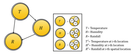
    semBnet extends standard Bayesian network analysis by incorporating domain knowledge, represented in terms of a semantic hierarchy [5]. In case of spatio-temporal prediction, semantic hierarchy is developed on the various concepts from the spatial domain and serves as the knowledge base to incorporate domain semantics in standard Bayesian analysis.

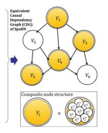
Typically, the semBnet consists of a qualitative component, comprising of a causal dependency graph (CDG), and a quantitative component, comprising of conditional probability distribution information for each of the nodes in the CDG.

Formally, the qualitative component of semBnet can be defined as a graph $G\left(V_{O}, V_{S}, E\right)$ which is directed as well as acyclic, where $V_{O}$ represents the set of nodes indicating random variables with no available semantics, $V_{S}$ represents the set of nodes indicating random variables with available semantics, and $E$ represents the set of edges between any two nodes in $\left(V_{O} \cup V_{S}\right)$. An edge from $V_{i} \in\left(V_{O} \cup V_{S}\right)$ to $V_{j} \in\left(V_{O} \cup V_{S}\right)$ indicates that variable $V_{i}$ influences variable $V_{j}$.
On the other side, the quantitative component of semBnet, i.e., the conditional probability distribution of any node $V_{x}$ in semBnet is represented as $P^{\uparrow}\left(V_{x} \mid\right.$ Parents $\left.\left(V_{x}\right)\right)$ if either $V_{x} \in V_{S}$ and/or $\left(\right.$ Parents $\left.\left(V_{x}\right) \cap V_{S}\right) \neq \emptyset$, where Parents $\left(V_{x}\right)$ denotes the set of parents or nodes influencing the target node $V_{x}$. Otherwise, the conditional probability is represented as that of the standard BN, i.e. $P\left(V_{x} \mid\right.$ Parents $\left.\left(V_{x}\right)\right)$.

统计代写|贝叶斯网络代写Bayesian network代考|Parameter Learning

This section illustrates the principle of semBnet learning in terms of marginal and conditional probability estimation.

For any node $V_{x} \in V_{O}$, the marginal probability $P\left(V_{x}\right)$ is estimated as that of a standard Bayesian network. However, if the node $V_{x}$ has available semantics (i.e. $V_{x} \in V_{S}$ ), the marginal probability is estimated as follows:
$$
P^{\dagger}\left(v_{x}\right)=\gamma \cdot\left[P\left(v_{x}\right)+\sum_{v_{x i}} S S\left(v_{x}, v_{x c}\right) \cdot P\left(v_{x c}\right)\right]
$$
where, $v_{x}$ and $v_{x c}$ are any two domain values corresponding to $V_{x} \in V_{S}$, so that $v_{x} \neq v_{x c} ; P\left(v_{x}\right)$ denotes the standard probability of $v_{x} ; \gamma$ is the normalization constant; and $S S\left(v_{x}, v_{x c}\right)$ denotes the semantic similarity between $v_{x}$ and $v_{x c}$

In order to estimate semantic similarity between any two concepts, semBnet needs the semantic knowledge base in the form of a semantic hierarchy (refer Fig.5.2). Assuming that a variable $X$ has semantic hierarchy available over its various concepts, the semantic similarity between any two of its concepts $x_{c_{1}}$ and $x_{c_{2}}$ is calculated as per the measure defined in [11] as follows.
$$
S S\left(x_{c_{1}}, x_{c_{2}}\right)=e^{-\delta l} \cdot \frac{e^{\lambda d}-e^{-\lambda . d}}{e^{\lambda d}+e^{-\lambda . d}}
$$
where, $d$ denotes the depth of subsumer (most immediate common ancestor) of the concept $x_{c_{1}}$ and $x_{c_{2}}$ in the semantic hierarchy; $l$ is the length of the shortest path between the concepts; $\lambda>0$ and $\delta \geq 0$ are control parameters that help to scale the contribution of $d$ and $l$, respectively. As mentioned in [11], usually, the $\lambda$ and $\delta$ are set to $0.6$ and $0.2$ respectively.

During conditional probability estimation, if the target variable $V_{x}$ does not have its semantic knowledge base available (i.e. $V_{x} \in V_{O}$ ) and neither of its parents has so (i.e. (Parent $\left.\left(V_{x}\right) \cap V_{S}\right)=\emptyset$ ), then the conditional probability distribution $P\left(V_{x} \mid\right.$ Parext $\left.\left(V_{x}\right)\right)$ is derived in the same way as that of standard BN. Otherwise, the available semantic information is utilized to estimate the conditional probabilities. Following are the three cases that can arise during conditional probability estimation in presence of domain semantics of at least one of the variables involved (target and/or its parents):
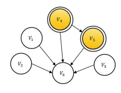
$\frac{\text { Case-I: } V_{x} \in V_{S} \text { and }\left(\text { Parents }\left(V_{x}\right) \cap V_{S}\right)=\emptyset:}{\text { Similar case arises for the variable } V_{S}^{4} \text { in Fig.5.3. }}$

统计代写|贝叶斯网络代写Bayesian network代考|semBnet-Based Prediction

Once the inferred probability distribution for the target/query variable is obtained, this is further processed to generate the predicted value of the variable. Considering the same example of rainfall prediction as described in the previous section, let $i n f e r_{R}^{s e m B n e t}$ is the semBnet inferred rainfall range corresponding to the highest probability estimate and infer standardBN is the standard Bayesian network inferred rainfall range corresponding to the highest probability estimate. Then $P^{\dagger}\left(i n f e r_{R}^{s e m} B n e t\right.$ $P\left(\right.$ infer ${ }{R}^{\text {standard } B N} \mid L U L C$, Elev, Lat $)=\max {i}\left{P\left(R_{i} \mid L U L C\right.\right.$, Elev, Lat $\left.)\right}$, where infer sembnet $=\left[L B_{R}^{\text {sem Bnet }}, U B_{R}^{\text {sem Bnet }}\right]$ and infer standard in $_{R}^{\text {s. }}=\left[L B_{R}^{\text {standard } B N}\right.$, $\left.U B_{R}^{\text {standard } B N}\right]$ (since the inferred values are in the form of ranges). Here $L B$ and $U B$ indicate the lower and upper bound of the range, respectively.
Then, the predicted value of Rainfall $\left(\mathrm{pred}{R}\right)$ is estimated as follows: $$ \text { pred }{R}=\left[\frac{L B_{R}^{\text {sem Bnet }}+L B_{R}^{\text {standardBN }}}{2}, \frac{U B_{R}^{\text {sem } B \text { net }}+U B_{R}^{\text {standard } B N}}{2}\right]=\left[L B_{R}^{\text {pred }}, U B_{R}^{\text {pred }}\right]
$$
In order to obtain a single value for Rainfall, one may use the mean of the predicted range: $\left(\frac{L B_{R}^{\text {pral }}+U B_{R}^{\text {preal }}}{2}\right)$.

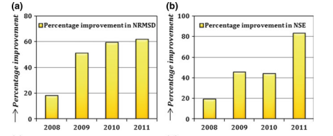
In the following part of the chapter, we attempt to present a case study to validate the effectiveness of semBnet-based prediction model in the presence of domain knowledge over the variables.

统计代写|贝叶斯网络代写Bayesian network代考|RE604

贝叶斯网络代考

统计代写|贝叶斯网络代写Bayesian network代考|Principle of semBnet

本节考虑 Sembnet 中描述的空间时间序列预测场景,从以下两个主要方面彻底解释 sembnet 的工作原理。5.3:

  • 参数学习
  • 推理生成
    semBnet 通过结合领域知识扩展了标准贝叶斯网络分析,领域知识以语义层次 [5] 表示。在时空预测的情况下,语义层次是在空间域的各种概念上开发的,并作为知识库将域语义合并到标准贝叶斯分析中。

通常,semBnet 由定性组件和定量组件组成,定性组件由因果依赖图 (CDG) 组成,定量组件由 CDG 中每个节点的条件概率分布信息组成。

形式上,semBnet 的定性组件可以定义为一个图G(在○,在小号,和)它是有向的和无环的,其中在○表示表示没有可用语义的随机变量的节点集,在小号表示表示具有可用语义的随机变量的节点集,并且和表示任意两个节点之间的边集(在○∪在小号). 一个边缘来自在一世∈(在○∪在小号)至在j∈(在○∪在小号)表示变量在一世影响变量在j.
另一方面,semBnet的量化分量,即任意节点的条件概率分布在X在 semBnet 中表示为磷↑(在X∣父母(在X))如果有的话在X∈在小号和/或(父母(在X)∩在小号)≠∅, 其中父母(在X)表示影响目标节点的父节点或节点集在X. 否则,条件概率表示为标准BN的条件概率,即磷(在X∣父母(在X)).

统计代写|贝叶斯网络代写Bayesian network代考|Parameter Learning

本节从边际和条件概率估计的角度说明 semBnet 学习的原理。

对于任何节点在X∈在○, 边际概率磷(在X)估计为标准贝叶斯网络的估计。但是,如果节点在X有可用的语义(即在X∈在小号),边际概率估计如下:

磷†(在X)=C⋅[磷(在X)+∑在X一世小号小号(在X,在XC)⋅磷(在XC)]
在哪里,在X和在XC是对应于的任意两个域值在X∈在小号, 以便在X≠在XC;磷(在X)表示标准概率在X;C是归一化常数;和小号小号(在X,在XC)表示之间的语义相似度在X和在XC

为了估计任意两个概念之间的语义相似度,semBnet 需要语义层次结构形式的语义知识库(见图 5.2)。假设一个变量X在其各种概念上具有可用的语义层次结构,其任意两个概念之间的语义相似性XC1和XC2根据 [11] 中定义的度量计算如下。

小号小号(XC1,XC2)=和−dl⋅和λd−和−λ.d和λd+和−λ.d
在哪里,d表示概念的包含深度(最直接的共同祖先)XC1和XC2在语义层次结构中;l是概念之间最短路径的长度;λ>0和d≥0是有助于衡量贡献的控制参数d和l, 分别。如 [11] 中所述,通常,λ和d设置为0.6和0.2分别。

在条件概率估计过程中,如果目标变量在X没有可用的语义知识库(即在X∈在○) 并且它的父母都没有这样 (即 (Parent(在X)∩在小号)=∅),然后是条件概率分布磷(在X∣帕雷克斯(在X))与标准 BN 的推导方式相同。否则,可用的语义信息被用来估计条件概率。以下是在存在至少一个所涉及变量(目标和/或其父项)的域语义的条件概率估计期间可能出现的三种情况:
 案例一: 在X∈在小号 和 ( 父母 (在X)∩在小号)=∅: 变量出现类似情况 在小号4 在图 5.3 中。 

统计代写|贝叶斯网络代写Bayesian network代考|semBnet-Based Prediction

一旦获得目标/查询变量的推断概率分布,就会对其进行进一步处理以生成变量的预测值。考虑与上一节中描述的降雨预测相同的例子,让一世nF和rRs和米乙n和吨是对应于最高概率估计的 semBnet 推断降雨范围,推断标准BN 是对应于最高概率估计的标准贝叶斯网络推断降雨范围。然后磷†(一世nF和rRs和米乙n和吨 磷(推断R标准 乙ñ∣大号在大号C, 海拔, 纬度)=\max {i}\left{P\left(R_{i} \mid L U L C\right.\right.$, Elev, Lat $\left.)\right})=\max {i}\left{P\left(R_{i} \mid L U L C\right.\right.$, Elev, Lat $\left.)\right}, 其中推断 sembnet=[大号乙R网络 ,在乙R网络 ]并推断标准Rs。 =[大号乙R标准 乙ñ, 在乙R标准 乙ñ](因为推断的值是范围的形式)。这里大号乙和在乙分别表示范围的下限和上限。
然后,Rainfall 的预测值(pr和dR)估计如下:

 前 R=[大号乙R网络 +大号乙R默认BN 2,在乙R扫描仪 乙 网 +在乙R标准 乙ñ2]=[大号乙R前 ,在乙R前 ]
为了获得 Rainfall 的单个值,可以使用预测范围的平均值:(大号乙R将要 +在乙R前级 2).

在本章的以下部分,我们尝试提出一个案例研究,以验证在变量存在领域知识的情况下,基于 semBnet 的预测模型的有效性。

统计代写|贝叶斯网络代写Bayesian network代考 请认准statistics-lab™

统计代写请认准statistics-lab™. statistics-lab™为您的留学生涯保驾护航。

金融工程代写

金融工程是使用数学技术来解决金融问题。金融工程使用计算机科学、统计学、经济学和应用数学领域的工具和知识来解决当前的金融问题,以及设计新的和创新的金融产品。

非参数统计代写

非参数统计指的是一种统计方法,其中不假设数据来自于由少数参数决定的规定模型;这种模型的例子包括正态分布模型和线性回归模型。

广义线性模型代考

广义线性模型(GLM)归属统计学领域,是一种应用灵活的线性回归模型。该模型允许因变量的偏差分布有除了正态分布之外的其它分布。

术语 广义线性模型(GLM)通常是指给定连续和/或分类预测因素的连续响应变量的常规线性回归模型。它包括多元线性回归,以及方差分析和方差分析(仅含固定效应)。

有限元方法代写

有限元方法(FEM)是一种流行的方法,用于数值解决工程和数学建模中出现的微分方程。典型的问题领域包括结构分析、传热、流体流动、质量运输和电磁势等传统领域。

有限元是一种通用的数值方法,用于解决两个或三个空间变量的偏微分方程(即一些边界值问题)。为了解决一个问题,有限元将一个大系统细分为更小、更简单的部分,称为有限元。这是通过在空间维度上的特定空间离散化来实现的,它是通过构建对象的网格来实现的:用于求解的数值域,它有有限数量的点。边界值问题的有限元方法表述最终导致一个代数方程组。该方法在域上对未知函数进行逼近。[1] 然后将模拟这些有限元的简单方程组合成一个更大的方程系统,以模拟整个问题。然后,有限元通过变化微积分使相关的误差函数最小化来逼近一个解决方案。

tatistics-lab作为专业的留学生服务机构,多年来已为美国、英国、加拿大、澳洲等留学热门地的学生提供专业的学术服务,包括但不限于Essay代写,Assignment代写,Dissertation代写,Report代写,小组作业代写,Proposal代写,Paper代写,Presentation代写,计算机作业代写,论文修改和润色,网课代做,exam代考等等。写作范围涵盖高中,本科,研究生等海外留学全阶段,辐射金融,经济学,会计学,审计学,管理学等全球99%专业科目。写作团队既有专业英语母语作者,也有海外名校硕博留学生,每位写作老师都拥有过硬的语言能力,专业的学科背景和学术写作经验。我们承诺100%原创,100%专业,100%准时,100%满意。

随机分析代写


随机微积分是数学的一个分支,对随机过程进行操作。它允许为随机过程的积分定义一个关于随机过程的一致的积分理论。这个领域是由日本数学家伊藤清在第二次世界大战期间创建并开始的。

时间序列分析代写

随机过程,是依赖于参数的一组随机变量的全体,参数通常是时间。 随机变量是随机现象的数量表现,其时间序列是一组按照时间发生先后顺序进行排列的数据点序列。通常一组时间序列的时间间隔为一恒定值(如1秒,5分钟,12小时,7天,1年),因此时间序列可以作为离散时间数据进行分析处理。研究时间序列数据的意义在于现实中,往往需要研究某个事物其随时间发展变化的规律。这就需要通过研究该事物过去发展的历史记录,以得到其自身发展的规律。

回归分析代写

多元回归分析渐进(Multiple Regression Analysis Asymptotics)属于计量经济学领域,主要是一种数学上的统计分析方法,可以分析复杂情况下各影响因素的数学关系,在自然科学、社会和经济学等多个领域内应用广泛。

MATLAB代写

MATLAB 是一种用于技术计算的高性能语言。它将计算、可视化和编程集成在一个易于使用的环境中,其中问题和解决方案以熟悉的数学符号表示。典型用途包括:数学和计算算法开发建模、仿真和原型制作数据分析、探索和可视化科学和工程图形应用程序开发,包括图形用户界面构建MATLAB 是一个交互式系统,其基本数据元素是一个不需要维度的数组。这使您可以解决许多技术计算问题,尤其是那些具有矩阵和向量公式的问题,而只需用 C 或 Fortran 等标量非交互式语言编写程序所需的时间的一小部分。MATLAB 名称代表矩阵实验室。MATLAB 最初的编写目的是提供对由 LINPACK 和 EISPACK 项目开发的矩阵软件的轻松访问,这两个项目共同代表了矩阵计算软件的最新技术。MATLAB 经过多年的发展,得到了许多用户的投入。在大学环境中,它是数学、工程和科学入门和高级课程的标准教学工具。在工业领域,MATLAB 是高效研究、开发和分析的首选工具。MATLAB 具有一系列称为工具箱的特定于应用程序的解决方案。对于大多数 MATLAB 用户来说非常重要,工具箱允许您学习应用专业技术。工具箱是 MATLAB 函数(M 文件)的综合集合,可扩展 MATLAB 环境以解决特定类别的问题。可用工具箱的领域包括信号处理、控制系统、神经网络、模糊逻辑、小波、仿真等。

R语言代写问卷设计与分析代写
PYTHON代写回归分析与线性模型代写
MATLAB代写方差分析与试验设计代写
STATA代写机器学习/统计学习代写
SPSS代写计量经济学代写
EVIEWS代写时间序列分析代写
EXCEL代写深度学习代写
SQL代写各种数据建模与可视化代写

统计代写|贝叶斯网络代写Bayesian network代考|ECSE4850

如果你也在 怎样代写贝叶斯网络Bayesian network这个学科遇到相关的难题,请随时右上角联系我们的24/7代写客服。

贝叶斯网络(BN)是一种表示不确定领域知识的概率图形模型,其中每个节点对应一个随机变量,每条边代表相应随机变量的条件概率。

statistics-lab™ 为您的留学生涯保驾护航 在代写贝叶斯网络Bayesian network方面已经树立了自己的口碑, 保证靠谱, 高质且原创的统计Statistics代写服务。我们的专家在代写贝叶斯网络Bayesian network代写方面经验极为丰富,各种代写贝叶斯网络Bayesian network相关的作业也就用不着说。

我们提供的贝叶斯网络Bayesian network及其相关学科的代写,服务范围广, 其中包括但不限于:

  • Statistical Inference 统计推断
  • Statistical Computing 统计计算
  • Advanced Probability Theory 高等概率论
  • Advanced Mathematical Statistics 高等数理统计学
  • (Generalized) Linear Models 广义线性模型
  • Statistical Machine Learning 统计机器学习
  • Longitudinal Data Analysis 纵向数据分析
  • Foundations of Data Science 数据科学基础
统计代写|贝叶斯网络代写Bayesian network代考|ECSE4850

统计代写|贝叶斯网络代写Bayesian network代考|Study Area and Dataset

The experimentation is carried out in the watershed and the associated reservoir of the river Mayurakshi in Jharkhand, India. The reservoir is located at the geographical position of $24^{\circ} 6.6^{\prime} \mathrm{N}$ latitude and $87^{\circ} 18.9^{\prime} E$ longitude (refer Tables $4.9$ and $4.10$ ) and the entire watershed covers nearly $1866 \mathrm{sq} . \mathrm{km}$ area (Bottom-Left: $\left[24.09^{\circ} N, 86.84^{\circ} E\right]$, Top-Right: $\left[24.62^{\circ} N, 87.40^{\circ} \mathrm{E}\right]$ ). The region has tropical climate, showing three well defined seasons: (i) summer: (March-June), (ii) rainy: (July-October), and (iii) winter: (November-February).

In order to experiment with SpaBN, the whole watershed region is considered to be distributed over $10 \times 10$ grid with each cell comprising approximately $33 \mathrm{sq} . \mathrm{km}$ area. The details of the datasets are specified below:

  • Rainfall: This is a daily rainfall data, interpolated for each of the gridded locations in the watershed for a span of 11 years (from 1st January, 1991 to 31 st December, 2001) The original daily data is available for four rain gauge stations (Jama $\left(24.35^{\circ} N, 87.15^{\circ} E\right)$, Dumka $\left(24.28^{\circ} N, 87.24^{\circ} E\right)$, Sariyahat $\left(24.58^{\circ} N, 87.01^{\circ} E\right)$,

and Jharmundi $\left(24.40^{\circ} \mathrm{N}, 87.05^{\circ} \mathrm{E}\right)$ ). Additionally, $0.5^{\circ} \times 0.5^{\circ}$ gridded rainfall data (refer Table 4.9) from Indian Meteorological Department (IMD) was also used for interpolation.

  • Temperature: This is a daily data of temperature, interpolated for each of the gridded locations, using original high resolution $1^{\circ} \times 1^{\circ}$ gridded temperature data (refer Table 4.9) from IMD.
  • Reservoir live/storage capacity: This data is collected from the office of Irrigation and Waterways Dept. Govt. of West Bengal, Kolkata, India, for the same duration (from 1st January, 1991 to 31 st December, 2001) [refer Table 4.10].
  • Topographical data: This includes slope map, soil map, and spatial distribution of land use land cover (LULC) (Fig.4.7) over the whole watershed. The original data of soil map and elevation map are available with National Bureau of Soil Survey and Land Use Planning, Govt of India. The LULC data is collected from Bhuvan portal [18]. It is evident from the maps that the watershed contains diverse LULC and soil categories. Almost $66 \%$ of the total area is agricultural crop land, and about $74 \%$ of the region is full of fine loamy soil.

统计代写|贝叶斯网络代写Bayesian network代考|Discussions

On analyzing the tables and the Fig. 4.10, we can infer the following about SpaBNbased prediction model:
(i) It is evident from the Tables $4.13,4.14,4.15$ and $4.16$ that the SpaBNbased approach produces the highest NSE value compared to statistical ARIMA, standard BN, and ANN models. Further, in almost all the cases, the value of NSE is approximately 1 . This indicates a highly accurate prediction made by SpaBN. Contrarily, the NSE values associated with the other prediction models, including standard BN, deviate quite significantly from 1. This demonstrates the preeminence of SpaBN-based prediction over the others, in carrying out spatial time series prediction.
(ii) It can also be noted that the values of NRMSD, computed for all the prediction years, are considerably low $(0.07-0.16)$ in case of SpaBN. This indicates the superiority of SpaBN[6] compared to the other techniques (refer Tables $4.13$, $4.14,4.15$ and 4.16). This also reveals the effectiveness of incorporating spatial information which eventually improves the accuracy for SpaBN-based prediction.
(iii) Besides, from the $\mathrm{D}_{v}$ and SEP values in Tables $4.13,4.14,4.15$ and $4.16$, it can be observed that SpaBN is more than $55 \%$ better than the statistical forecasting models, and almost $25 \%$ better than the ANN-based prediction technique on average. Further, with respect to the standard BNs that handles no spatial information, the performance of SpaBN-based approach is improved about $13 \%$.
(iv) From the Tables $4.13,4.14,4.15$ and $4.16$, we can also find that in most of the cases, the SpaBN provides a high $R^{2}$ value $\sim 1$, whereas the $R^{2}$ value for the ARIMA models, ANN, and standard BN are $\sim 0.0,0.3$, and $0.6$, respectively. In general, the $R^{2}$ values range between 0 and 1 , and these are indicators of fitness of the prediction methods. The higher the value of $R^{2}$, the better the model fits for prediction. Therefore, the high $R^{2}$ value corresponding to SpaBN demonstrates that the model is desirably fit for the hydrological time series prediction.
(v) The comparative study of the model forecasts and the actual/observed daily reservoir live capacities for all the prediction years 1998-2001 are shown in the Fig. 4.10. It is evident from the figure that the predicted time series of SpaBN-based prediction model is matching well with the actual/observed value of live capacity in all the cases, indicating effectiveness of the model. From the Fig. 4.10, it can be also observed that, whenever there is over estimation or under-estimation generated from standard BN, the SpaBN has a notable tendency to improve this by making it as near to the observed value as possible [6]. Consideration of additional predictors like evapotranspiration, evaporation etc. from the reservoir water surface and watershed may further improve the model performance.

统计代写|贝叶斯网络代写Bayesian network代考|Existing Variants of Semantic Bayesian Network

The idea of incorporating domain semantics in Bayesian network is not very new. Different variants of semantic Bayesian networks $[2,9,12,15,20]$ have shown their effectiveness in several application areas. However, Bayesian networks with embedded semantics from spatial domain is still a little explored topic.
The semantic Bayesian network (SeBN) [9] proposed by Kim et al. is intended for conversational agent to infer the detailed intentions of the user. The SeBN itself maintains probabilistic as well as semantic relationships and the inference generation is followed from a thresholding process that helps in selecting target value appropriate for the user query. The sBN is another variant of semantic Bayesian network proposed by Zhou et al. [20] for constructing web mashup network. sBN is utilized here to process the information from semantic web. In order to describe the information on the graph structure and facilitate processing of semantic graph structure-based attributes, the authors use a semantic subgraph template defined using SPARQL query. There also exist some research works exploiting semantics while generating inference using Bayesian network. The works by Butz et al. $[2,12]$ are worth mentioning in this context. In [2], the authors propose a join tree probability propagation architecture for conducting the semantically enhanced inference generation from BN. The architecture is defined in such a way that each node in the join tree maintains a local BN preserving all conditional independencies of the original Bayesian network. In the work of Madsen and Butz [12], the authors use a lazy Propagation model for capturing semantics of potentials created during belief updating process. The model employs a combination of Shenoy-Shafer propagation [13] and variable elimination scheme to help in computing messages and marginals.

Recently, Das and Ghosh [5] have proposed a new variant of semantic Bayesian network, termed as semBnet, which is also applicable for spatial time series prediction [5]. This can be considered as the first work that uses semantically enhanced BN model for multivariate time series prediction in spatial domain. The overall working principle of semBnet is grounded on semantic hierarchy, a hierarchical representation of domain knowledge from which semBnet is able to extract the semantic similarity between various spatial concepts and can utilize the same in the Bayesian analysis process.

统计代写|贝叶斯网络代写Bayesian network代考|ECSE4850

贝叶斯网络代考

统计代写|贝叶斯网络代写Bayesian network代考|Study Area and Dataset

该实验在印度贾坎德邦的 Mayurakshi 河的分水岭和相关水库中进行。水库位于地理位置24∘6.6′ñ纬度和87∘18.9′和经度(参考表4.9和4.10),整个流域几乎覆盖1866sq.ķ米区域(左下:[24.09∘ñ,86.84∘和], 右上:[24.62∘ñ,87.40∘和])。该地区具有热带气候,表现出三个明确的季节:(i)夏季:(3 月至 6 月),(ii)多雨:(7 月至 10 月)和(iii)冬季:(11 月至 2 月)。

为了试验 SpaBN,整个流域区域被认为分布在10×10每个单元格包含大约33sq.ķ米区域。数据集的详细信息如下:

  • 降雨量:这是一个每日降雨量数据,在 11 年(从 1991 年 1 月 1 日至 2001 年 12 月 31 日)内为流域中的每个网格位置插值(从 1991 年 1 月 1 日到 2001 年 12 月 31 日)原始每日数据可用于四个雨量站(贾马(24.35∘ñ,87.15∘和), 杜姆卡(24.28∘ñ,87.24∘和), 萨里亚哈特(24.58∘ñ,87.01∘和),

和贾尔蒙迪(24.40∘ñ,87.05∘和))。此外,0.5∘×0.5∘印度气象局 (IMD) 的网格化降雨数据(参见表 4.9)也用于插值。

  • 温度:这是每日的温度数据,使用原始高分辨率对每个网格位置进行插值1∘×1∘来自 IMD 的网格温度数据(参见表 4.9)。
  • 水库活/蓄水能力:该数据是从灌溉和水道部政府办公室收集的。印度加尔各答的西孟加拉邦,同样的时间(从 1991 年 1 月 1 日到 2001 年 12 月 31 日)[参见表 4.10]。
  • 地形数据:包括坡度图、土壤图和整个流域土地利用土地覆被(LULC)的空间分布(图 4.7)。土壤图和海拔图的原始数据可从印度政府国家土壤调查和土地利用规划局获得。LULC 数据是从 Bhuvan 门户网站 [18] 收集的。从地图上可以明显看出,流域包含不同的 LULC 和土壤类别。几乎66%总面积的一半是农田,大约74%该地区充满了细壤土。

统计代写|贝叶斯网络代写Bayesian network代考|Discussions

通过分析表格和图 4.10,我们可以推断出基于 SpaBN 的预测模型如下:
(i) 从表格中可以看出4.13,4.14,4.15和4.16与统计 ARIMA、标准 BN 和 ANN 模型相比,基于 SpaBN 的方法产生最高的 NSE 值。此外,几乎在所有情况下,NSE 的值都约为 1。这表明 SpaBN 做出了高度准确的预测。相反,与包括标准 BN 在内的其他预测模型相关的 NSE 值与 1 有很大的偏差。这证明了基于 SpaBN 的预测在执行空间时间序列预测时优于其他预测模型。
(ii) 还可以注意到,针对所有预测年份计算的 NRMSD 值相当低(0.07−0.16)在 SpaBN 的情况下。这表明 SpaBN[6] 与其他技术相比具有优势(参见表4.13, 4.14,4.15和 4.16)。这也揭示了结合空间信息的有效性,最终提高了基于 SpaBN 的预测的准确性。
(iii) 此外,从D在和表中的 SEP 值4.13,4.14,4.15和4.16, 可以看出 SpaBN 大于55%比统计预测模型好,而且几乎25%平均而言,优于基于 ANN 的预测技术。此外,对于不处理空间信息的标准 BN,基于 SpaBN 的方法的性能提高了大约13%.
(iv) 从表格4.13,4.14,4.15和4.16,我们还可以发现,在大多数情况下,SpaBN 提供了很高的R2价值∼1,而R2ARIMA 模型、ANN 和标准 BN 的值是∼0.0,0.3, 和0.6, 分别。一般来说,R2值范围在 0 和 1 之间,这些是预测方法的适应度指标。的价值越高R2,模型越适合预测。因此,高R2对应于 SpaBN 的值表明该模型非常适合水文时间序列预测。
(v) 1998-2001 年所有预测年份的模型预测与实际/观测的水库日活容量对比研究见图 4.10。从图中可以明显看出,基于 SpaBN 的预测模型的预测时间序列在所有情况下都与实际/观察到的活量值很好地匹配,表明了模型的有效性。从图 4.10 还可以观察到,每当标准 BN 产生高估或低估时,SpaBN 具有通过使其尽可能接近观察值来改善这一点的显着趋势 [6] . 考虑来自水库水面和流域的其他预测因子,如蒸发量、蒸发量等,可以进一步提高模型性能。

统计代写|贝叶斯网络代写Bayesian network代考|Existing Variants of Semantic Bayesian Network

在贝叶斯网络中加入域语义的想法并不是很新。语义贝叶斯网络的不同变体[2,9,12,15,20]已在多个应用领域显示出其有效性。然而,具有来自空间域的嵌入语义的贝叶斯网络仍然是一个小小的探索主题。
Kim等人提出的语义贝叶斯网络(SeBN)[9]。旨在让会话代理推断用户的详细意图。SeBN 本身维护概率关系和语义关系,并且推理生成是从有助于选择适合用户查询的目标值的阈值处理之后进行的。sBN 是 Zhou 等人提出的语义贝叶斯网络的另一种变体。[20] 用于构建 web mashup 网络。这里使用 sBN 来处理来自语义网络的信息。为了描述关于图结构的信息并促进基于语义图结构的属性的处理,作者使用了使用 SPARQL 查询定义的语义子图模板。也有一些研究工作在利用贝叶斯网络生成推理的同时利用语义。Butz 等人的作品。[2,12]在这方面值得一提。在 [2] 中,作者提出了一种连接树概率传播架构,用于从 BN 进行语义增强的推理生成。该架构以这样一种方式定义,即连接树中的每个节点都维护一个本地 BN,保留原始贝叶斯网络的所有条件独立性。在 Madsen 和 Butz [12] 的工作中,作者使用惰性传播模型来捕获在信念更新过程中创建的势的语义。该模型采用 Shenoy-Shafer 传播 [13] 和变量消除方案的组合来帮助计算消息和边缘。

最近,Das 和 Ghosh [5] 提出了语义贝叶斯网络的一种新变体,称为 semBnet,它也适用于空间时间序列预测 [5]。这可以被认为是第一个使用语义增强的 BN 模型在空间域中进行多变量时间序列预测的工作。semBnet 的总体工作原理是基于语义层次结构,这是一种领域知识的层次表示,semBnet 能够从中提取各种空间概念之间的语义相似性,并可以在贝叶斯分析过程中加以利用。

统计代写|贝叶斯网络代写Bayesian network代考 请认准statistics-lab™

统计代写请认准statistics-lab™. statistics-lab™为您的留学生涯保驾护航。

金融工程代写

金融工程是使用数学技术来解决金融问题。金融工程使用计算机科学、统计学、经济学和应用数学领域的工具和知识来解决当前的金融问题,以及设计新的和创新的金融产品。

非参数统计代写

非参数统计指的是一种统计方法,其中不假设数据来自于由少数参数决定的规定模型;这种模型的例子包括正态分布模型和线性回归模型。

广义线性模型代考

广义线性模型(GLM)归属统计学领域,是一种应用灵活的线性回归模型。该模型允许因变量的偏差分布有除了正态分布之外的其它分布。

术语 广义线性模型(GLM)通常是指给定连续和/或分类预测因素的连续响应变量的常规线性回归模型。它包括多元线性回归,以及方差分析和方差分析(仅含固定效应)。

有限元方法代写

有限元方法(FEM)是一种流行的方法,用于数值解决工程和数学建模中出现的微分方程。典型的问题领域包括结构分析、传热、流体流动、质量运输和电磁势等传统领域。

有限元是一种通用的数值方法,用于解决两个或三个空间变量的偏微分方程(即一些边界值问题)。为了解决一个问题,有限元将一个大系统细分为更小、更简单的部分,称为有限元。这是通过在空间维度上的特定空间离散化来实现的,它是通过构建对象的网格来实现的:用于求解的数值域,它有有限数量的点。边界值问题的有限元方法表述最终导致一个代数方程组。该方法在域上对未知函数进行逼近。[1] 然后将模拟这些有限元的简单方程组合成一个更大的方程系统,以模拟整个问题。然后,有限元通过变化微积分使相关的误差函数最小化来逼近一个解决方案。

tatistics-lab作为专业的留学生服务机构,多年来已为美国、英国、加拿大、澳洲等留学热门地的学生提供专业的学术服务,包括但不限于Essay代写,Assignment代写,Dissertation代写,Report代写,小组作业代写,Proposal代写,Paper代写,Presentation代写,计算机作业代写,论文修改和润色,网课代做,exam代考等等。写作范围涵盖高中,本科,研究生等海外留学全阶段,辐射金融,经济学,会计学,审计学,管理学等全球99%专业科目。写作团队既有专业英语母语作者,也有海外名校硕博留学生,每位写作老师都拥有过硬的语言能力,专业的学科背景和学术写作经验。我们承诺100%原创,100%专业,100%准时,100%满意。

随机分析代写


随机微积分是数学的一个分支,对随机过程进行操作。它允许为随机过程的积分定义一个关于随机过程的一致的积分理论。这个领域是由日本数学家伊藤清在第二次世界大战期间创建并开始的。

时间序列分析代写

随机过程,是依赖于参数的一组随机变量的全体,参数通常是时间。 随机变量是随机现象的数量表现,其时间序列是一组按照时间发生先后顺序进行排列的数据点序列。通常一组时间序列的时间间隔为一恒定值(如1秒,5分钟,12小时,7天,1年),因此时间序列可以作为离散时间数据进行分析处理。研究时间序列数据的意义在于现实中,往往需要研究某个事物其随时间发展变化的规律。这就需要通过研究该事物过去发展的历史记录,以得到其自身发展的规律。

回归分析代写

多元回归分析渐进(Multiple Regression Analysis Asymptotics)属于计量经济学领域,主要是一种数学上的统计分析方法,可以分析复杂情况下各影响因素的数学关系,在自然科学、社会和经济学等多个领域内应用广泛。

MATLAB代写

MATLAB 是一种用于技术计算的高性能语言。它将计算、可视化和编程集成在一个易于使用的环境中,其中问题和解决方案以熟悉的数学符号表示。典型用途包括:数学和计算算法开发建模、仿真和原型制作数据分析、探索和可视化科学和工程图形应用程序开发,包括图形用户界面构建MATLAB 是一个交互式系统,其基本数据元素是一个不需要维度的数组。这使您可以解决许多技术计算问题,尤其是那些具有矩阵和向量公式的问题,而只需用 C 或 Fortran 等标量非交互式语言编写程序所需的时间的一小部分。MATLAB 名称代表矩阵实验室。MATLAB 最初的编写目的是提供对由 LINPACK 和 EISPACK 项目开发的矩阵软件的轻松访问,这两个项目共同代表了矩阵计算软件的最新技术。MATLAB 经过多年的发展,得到了许多用户的投入。在大学环境中,它是数学、工程和科学入门和高级课程的标准教学工具。在工业领域,MATLAB 是高效研究、开发和分析的首选工具。MATLAB 具有一系列称为工具箱的特定于应用程序的解决方案。对于大多数 MATLAB 用户来说非常重要,工具箱允许您学习应用专业技术。工具箱是 MATLAB 函数(M 文件)的综合集合,可扩展 MATLAB 环境以解决特定类别的问题。可用工具箱的领域包括信号处理、控制系统、神经网络、模糊逻辑、小波、仿真等。

R语言代写问卷设计与分析代写
PYTHON代写回归分析与线性模型代写
MATLAB代写方差分析与试验设计代写
STATA代写机器学习/统计学习代写
SPSS代写计量经济学代写
EVIEWS代写时间序列分析代写
EXCEL代写深度学习代写
SQL代写各种数据建模与可视化代写

统计代写|贝叶斯网络代写Bayesian network代考|CSCl252

如果你也在 怎样代写贝叶斯网络Bayesian network这个学科遇到相关的难题,请随时右上角联系我们的24/7代写客服。

贝叶斯网络(BN)是一种表示不确定领域知识的概率图形模型,其中每个节点对应一个随机变量,每条边代表相应随机变量的条件概率。

statistics-lab™ 为您的留学生涯保驾护航 在代写贝叶斯网络Bayesian network方面已经树立了自己的口碑, 保证靠谱, 高质且原创的统计Statistics代写服务。我们的专家在代写贝叶斯网络Bayesian network代写方面经验极为丰富,各种代写贝叶斯网络Bayesian network相关的作业也就用不着说。

我们提供的贝叶斯网络Bayesian network及其相关学科的代写,服务范围广, 其中包括但不限于:

  • Statistical Inference 统计推断
  • Statistical Computing 统计计算
  • Advanced Probability Theory 高等概率论
  • Advanced Mathematical Statistics 高等数理统计学
  • (Generalized) Linear Models 广义线性模型
  • Statistical Machine Learning 统计机器学习
  • Longitudinal Data Analysis 纵向数据分析
  • Foundations of Data Science 数据科学基础
统计代写|贝叶斯网络代写Bayesian network代考|CSCl252

统计代写|贝叶斯网络代写Bayesian network代考|Why SpaBN for Spatial Time Series Prediction

Spatio-temporal variables are not independent. In most of the cases, these are dependent on various other co-located variables. For example, consider a scenario

of predicting water level at a reservoir in the flow of any river. The water level at the reservoir depends on many factors, like the volume of inflow and outflow of water, seepage into ground, evaporation, meteorological condition, and so on. One of the significant meteorological factors in this regard is the environmental precipitation. Now, the level of water in the reservoir depends not only on the precipitation at the reservoir location, but also that in the various other locations in the whole watershed of the corresponding river. Moreover, based on the various topographical factors, like soil type, land cover category, land slope etc., the precipitation at the different locations may have different influence on the water level of the reservoir. Thus, modeling the spatial effect/influence of precipitation or any such meteorological factor on the reservoir water level becomes a challenging issue, inasmuch as the watershed of any river is in general large and consists of locations with varying topographic characteristics.

Although the graphical models, like Bayesian networks, are highly suitable for representing such inter-variable influences, yet, for each such influencing variable, introducing representative node corresponding to each spatial location will lead to a very complicated causal dependency graph structure consisting of a large number of nodes and edges. One such example scenario has been illustrated through the Fig. 4.3, which shows a graphical model representing influence from three variables $V_{i}$, $(i=1,2,3)$, distributed at $K=8$ number of spatial locations. This eventually leads to extremely high time and space complexities during parameter learning and inference process. The spatial Bayesian network (SpaBN) can handle this situation efficiently, by using the composite node representation for each spatially distributed variable.

统计代写|贝叶斯网络代写Bayesian network代考|Parameter Learning

Let us assume a directed acyclic graph $G\left(V_{s}, V_{c}, E\right)$, as shown in the Fig. 4.1, where $V_{s}=\left{V_{2}, V_{6}\right}$ denotes the set of standard nodes; $V_{c}=\left{V_{1}, V_{3}, V_{4}, V_{5}\right}$ denotes the set of composite nodes; and $E$ is the set of edges $\left{V_{1} \rightarrow V_{2}, V_{1} \rightarrow\right.$ $\left.V_{3}, \quad V_{1} \rightarrow V_{4}, V_{2} \rightarrow V_{4}, V_{2} \rightarrow V_{5}, V_{3} \rightarrow V_{4}, V_{3} \rightarrow V_{6}, V_{4} \rightarrow V_{5}, V_{4} \rightarrow V_{6}\right}$. An edge from $V_{i}$ to $V_{j}$ can be interpreted as $V_{i}$ has influence on $V_{j}$. Let us also consider that the variables corresponding to the composite nodes are spatially distributed over $K$ ( $=8$ as per the figure) number of locations.

According to the learning principle of SpaBN $[6]$, the marginal probabilities of the composite nodes $\in V_{c}$ in this scenario are calculated with consideration to the spatial importance of each neighboring location:
$$
\begin{aligned}
&\boldsymbol{P}\left(V_{1}\right)=\gamma \cdot\left[\sum_{i=1}^{K} P\left(V_{1}^{i}\right) \cdot S W_{i}\right] \
&P\left(V_{3}\right)=\gamma \cdot\left[\sum_{i=1}^{K} P\left(V_{3}^{i}\right) \cdot S W_{i}\right] \
&P\left(V_{4}\right)=\gamma \cdot\left[\sum_{i=1}^{K} P\left(V_{4}^{i}\right) \cdot S W_{i}\right] \
&P\left(V_{5}\right)=\gamma \cdot\left[\sum_{i=1}^{K} P\left(V_{5}^{i}\right) \cdot S W_{i}\right]
\end{aligned}
$$
where, $\gamma$ is a normalization constant such that the sum of marginal probabilities corresponding to all possible values of the variable becomes $1 . P\left(V_{j}^{i}\right)$ is the marginal probability of singular component $V_{j}^{i}$ in $V_{j}$, for $\mathrm{j}=1,3,4,5$, and $S W_{i}$ is the spatial weight/importance of the $i$ th neighboring location. For example, considering

the example scenario in the Chap. 1 (Fig. 1.2) and assuming the prediction location is Location-3, the probability distribution for the variable $T$ for the year 2011 can be estimated as: $P(T 1)=\gamma \cdot\left[\left(T_{1}^{\text {Locl }} \times S W_{L o c 1}\right)+\left(T_{1}^{\text {Loc } 2} \times S W_{L o c 2}\right)+\left(T_{1}^{\text {Loc } 3} \times\right.\right.$ $\left.\left.S W_{\text {Lac3 }}\right)\right]=\gamma \cdot[(0.8 \times 0.03)+(0.0 \times 0.97)+(0.0 \times 1.0)]=0.024 \gamma$. In similar way, we can estimate $P(T 2)=0.006 \gamma, P(T 3)=0.2 \gamma, P(T 4)=1.38 \gamma$, and $P(T 5)=0.39 \gamma$, where $\gamma$ is the normalization constant and can be determined as $0.5$. Thus, the normalized probability distribution for the spatially distributed variable $T$ becomes $P(T 1)=0.012, P(T 2)=0.003, P(T 3)=0.1, P(T 4)=0.69$, $P(T 5)=0.195$

The conditional probabilities, involving composite nodes $\in V_{c}$, are calculated similarly, considering spatial importance of the nearby locations, as follows:
$$
\begin{aligned}
P\left(V_{2} \mid V_{1}\right)=\gamma \cdot & {\left[\sum_{i=1}^{K} \frac{n\left(V_{2}, V_{1}^{i}\right)}{n\left(V_{1}^{i}\right)} \cdot S W_{i}\right] } \
P\left(V_{3} \mid V_{1}\right)=\gamma \cdot & {\left[\sum_{i=1}^{K} \frac{n\left(V_{3}^{i}, V_{1}^{i}\right)}{n\left(V_{1}^{i}\right)} \cdot S W_{i}\right] } \
P\left(V_{4} \mid V_{1}, V_{2}, V_{3}\right)=\gamma \cdot & {\left[\sum_{i=1}^{K} \frac{n\left(V_{1}^{i}, V_{2}, V_{3}^{i}, V_{4}^{i}\right)}{n\left(V_{1}^{i}, V_{2}, V_{3}^{i}\right)} \cdot S W_{i}\right] } \
P\left(V_{5} \mid V_{2}, V_{4}\right)=\gamma \cdot & {\left[\sum_{i=1}^{K} \frac{n\left(V_{5}^{i}, V_{2}, V_{4}^{i}\right)}{n\left(V_{2}, V_{4}^{i}\right)} \cdot S W_{i}\right] } \
P\left(V_{6} \mid V_{3}, V_{4}\right)=\gamma \cdot & {\left[\sum_{i=1}^{K} \frac{n\left(V_{6}, V_{3}^{i}, V_{4}^{i}\right)}{n\left(V_{3}^{i}, V_{4}^{i}\right)}-S W_{i}\right] }
\end{aligned}
$$
where, $n(<,>)$ represents the total number of observation for the variable combination $<\cdot>$. Considering the example scenario presented in Chap. 1 (Fig. 1.2) and assuming the prediction location to be Location-3, the calculation of conditional probability distribution of the variable humidity $(H)$ for the year 2011 are explained through Fig. 4.4, in comparison with standard BN based probability calculation. Here, the structure of SpaBN is considered to be as depicted in Fig. 4.2.

It is to be noted that the causal dependency graph of the SpaBN does not contain any of the spatial attributes (SAs) as described while discussing ST relationship learning in the Chap. 3. Rather, for any variable under study, the network considers relevant node corresponding to each of the associated spatial locations explicitly, and the appropriate spatial attributes are utilized in spatial weight/importance $(S W)$ calculation. The overall process of ST relationship learning using SpaBN is presented through the Algorithm $3 .$

统计代写|贝叶斯网络代写Bayesian network代考|SpaBN-Based Prediction

Once the inferred value is produced, it is further processed to finally generate the predicted value of the variable. Among all the inferred values of the prediction variable, the predicted value becomes the one which is associated with the highest probability estimates $P(\cdot)$. Therefore, if pred $V_{j}$ is the predicted value of the variable $V_{j}$, then $P\left(\operatorname{pred}{V{j}} \mid e\right)=\max \left{P\left(V_{j} \mid e\right)\right}$, where $e$ indicates the given combination of values for the set of evidence variables, and $P\left(V_{j} \mid e\right)$ represents the inferred probability distribution of the variable $V_{j}$ given $e$. With respect to the above example, $P\left(\right.$ pred $\left.V_{6} \mid V_{1}, V_{2}, \ldots, V_{4}\right)=\max \left{P\left(V_{6} \mid V_{1}, V_{2}, \ldots, V_{4}\right)\right}$. Now, since the overall SpaBN analysis is performed considering discretized value of the variables, the predicted value pred ${ }{V j}$ is also obtained in the form of range of values $\left[L B{j}, U B_{j}\right]$. Hence, in order to obtained a single value for the prediction variable, the mid value of the range may be considered. Therefore, finally, $\operatorname{pred}{V{j}}=\left(L B_{j}+U B_{j}\right) / 2$

统计代写|贝叶斯网络代写Bayesian network代考|CSCl252

贝叶斯网络代考

统计代写|贝叶斯网络代写Bayesian network代考|Why SpaBN for Spatial Time Series Prediction

时空变量不是独立的。在大多数情况下,这些取决于各种其他位于同一位置的变量。例如,考虑一个场景

预测任何河流中水库的水位。水库的水位取决于许多因素,如进出水量、渗入地下、蒸发量、气象条件等。这方面的重要气象因素之一是环境降水。现在,水库的水位不仅取决于水库所在地的降水量,还取决于相应河流整个流域内其他各个位置的降水量。此外,根据土壤类型、土地覆被类型、坡度等各种地形因素,不同地点的降水对水库水位的影响可能不同。因此,

尽管像贝叶斯网络这样的图形模型非常适合表示这种变量间的影响,但是,对于每个这样的影响变量,引入与每个空间位置对应的代表节点将导致一个非常复杂的因果依赖图结构,该结构由一个大的节点和边的数量。图 4.3 说明了一个这样的示例场景,该图显示了一个图形模型,表示三个变量的影响在一世, (一世=1,2,3), 分布在ķ=8空间位置的数量。这最终导致参数学习和推理过程中的时间和空间复杂性极高。空间贝叶斯网络 (SpaBN) 可以通过对每个空间分布变量使用复合节点表示来有效地处理这种情况。

统计代写|贝叶斯网络代写Bayesian network代考|Parameter Learning

让我们假设一个有向无环图G(在s,在C,和),如图 4.1 所示,其中V_{s}=\left{V_{2}, V_{6}\right}V_{s}=\left{V_{2}, V_{6}\right}表示标准节点的集合;V_{c}=\left{V_{1}, V_{3}, V_{4}, V_{5}\right}V_{c}=\left{V_{1}, V_{3}, V_{4}, V_{5}\right}表示复合节点的集合;和和是边的集合\left{V_{1} \rightarrow V_{2}, V_{1} \rightarrow\right.$ $\left.V_{3}, \quad V_{1} \rightarrow V_{4}, V_{2} \rightarrow V_{4}, V_{2} \rightarrow V_{5}, V_{3} \rightarrow V_{4}, V_{3} \rightarrow V_{6}, V_{4} \rightarrow V_{5} , V_{4} \rightarrow V_{6}\right}\left{V_{1} \rightarrow V_{2}, V_{1} \rightarrow\right.$ $\left.V_{3}, \quad V_{1} \rightarrow V_{4}, V_{2} \rightarrow V_{4}, V_{2} \rightarrow V_{5}, V_{3} \rightarrow V_{4}, V_{3} \rightarrow V_{6}, V_{4} \rightarrow V_{5} , V_{4} \rightarrow V_{6}\right}. 一个边缘来自在一世至在j可以解释为在一世有影响在j. 让我们还考虑对应于复合节点的变量在空间上分布在ķ ( =8如图)位置的数量。

根据SpaBN的学习原理[6], 复合节点的边际概率∈在C在这种情况下,计算时会考虑每个相邻位置的空间重要性:

磷(在1)=C⋅[∑一世=1ķ磷(在1一世)⋅小号在一世] 磷(在3)=C⋅[∑一世=1ķ磷(在3一世)⋅小号在一世] 磷(在4)=C⋅[∑一世=1ķ磷(在4一世)⋅小号在一世] 磷(在5)=C⋅[∑一世=1ķ磷(在5一世)⋅小号在一世]
在哪里,C是一个归一化常数,使得对应于变量所有可能值的边际概率之和变为1.磷(在j一世)是奇异分量的边际概率在j一世在在j, 为了j=1,3,4,5, 和小号在一世是空间权重/重要性一世th 相邻位置。例如,考虑

章节中的示例场景。1(图 1.2)并假设预测位置是 Location-3,变量的概率分布吨2011 年可估算为:磷(吨1)=C⋅[(吨1本地 ×小号在大号○C1)+(吨1地方 2×小号在大号○C2)+(吨1地方 3× 小号在紫胶3 )]=C⋅[(0.8×0.03)+(0.0×0.97)+(0.0×1.0)]=0.024C. 类似地,我们可以估计磷(吨2)=0.006C,磷(吨3)=0.2C,磷(吨4)=1.38C, 和磷(吨5)=0.39C, 在哪里C是归一化常数,可以确定为0.5. 因此,空间分布变量的归一化概率分布吨变成磷(吨1)=0.012,磷(吨2)=0.003,磷(吨3)=0.1,磷(吨4)=0.69, 磷(吨5)=0.195

条件概率,涉及复合节点∈在C, 计算类似,考虑到附近位置的空间重要性,如下所示:

磷(在2∣在1)=C⋅[∑一世=1ķn(在2,在1一世)n(在1一世)⋅小号在一世] 磷(在3∣在1)=C⋅[∑一世=1ķn(在3一世,在1一世)n(在1一世)⋅小号在一世] 磷(在4∣在1,在2,在3)=C⋅[∑一世=1ķn(在1一世,在2,在3一世,在4一世)n(在1一世,在2,在3一世)⋅小号在一世] 磷(在5∣在2,在4)=C⋅[∑一世=1ķn(在5一世,在2,在4一世)n(在2,在4一世)⋅小号在一世] 磷(在6∣在3,在4)=C⋅[∑一世=1ķn(在6,在3一世,在4一世)n(在3一世,在4一世)−小号在一世]
在哪里,n(<,>)表示变量组合的观察总数<⋅>. 考虑第 1 章中介绍的示例场景。1(图1.2)假设预测位置为Location-3,计算变量湿度的条件概率分布(H)2011 年通过图 4.4 解释,与基于标准 BN 的概率计算进行比较。这里,SpaBN 的结构被认为如图 4.2 所示。

需要注意的是,SpaBN 的因果依赖图不包含任何空间属性(SA),正如在第 1 章中讨论 ST 关系学习时所描述的那样。3. 相反,对于研究中的任何变量,网络明确考虑与每个相关空间位置对应的相关节点,并在空间权重/重要性中使用适当的空间属性(小号在)计算。通过算法呈现使用SpaBN进行ST关系学习的整体过程3.

统计代写|贝叶斯网络代写Bayesian network代考|SpaBN-Based Prediction

一旦产生了推断值,它会被进一步处理以最终生成变量的预测值。在预测变量的所有推断值中,预测值成为与最高概率估计相关联的值磷(⋅). 因此,如果预在j是变量的预测值在j, 然后P\left(\operatorname{pred}{V{j}} \mid e\right)=\max \left{P\left(V_{j} \mid e\right)\right}P\left(\operatorname{pred}{V{j}} \mid e\right)=\max \left{P\left(V_{j} \mid e\right)\right}, 在哪里和表示一组证据变量的给定值组合,并且磷(在j∣和)表示变量的推断概率分布在j给定和. 对于上面的例子,磷(前\left.V_{6} \mid V_{1}, V_{2}, \ldots, V_{4}\right)=\max \left{P\left(V_{6} \mid V_{1}, V_{2}, \ldots, V_{4}\right)\right}\left.V_{6} \mid V_{1}, V_{2}, \ldots, V_{4}\right)=\max \left{P\left(V_{6} \mid V_{1}, V_{2}, \ldots, V_{4}\right)\right}. 现在,由于整体 SpaBN 分析是考虑变量的离散值进行的,因此预测值 pred在j也以取值范围的形式得到[大号乙j,在乙j]. 因此,为了获得预测变量的单个值,可以考虑范围的中间值。因此,最后,前⁡在j=(大号乙j+在乙j)/2

统计代写|贝叶斯网络代写Bayesian network代考 请认准statistics-lab™

统计代写请认准statistics-lab™. statistics-lab™为您的留学生涯保驾护航。

金融工程代写

金融工程是使用数学技术来解决金融问题。金融工程使用计算机科学、统计学、经济学和应用数学领域的工具和知识来解决当前的金融问题,以及设计新的和创新的金融产品。

非参数统计代写

非参数统计指的是一种统计方法,其中不假设数据来自于由少数参数决定的规定模型;这种模型的例子包括正态分布模型和线性回归模型。

广义线性模型代考

广义线性模型(GLM)归属统计学领域,是一种应用灵活的线性回归模型。该模型允许因变量的偏差分布有除了正态分布之外的其它分布。

术语 广义线性模型(GLM)通常是指给定连续和/或分类预测因素的连续响应变量的常规线性回归模型。它包括多元线性回归,以及方差分析和方差分析(仅含固定效应)。

有限元方法代写

有限元方法(FEM)是一种流行的方法,用于数值解决工程和数学建模中出现的微分方程。典型的问题领域包括结构分析、传热、流体流动、质量运输和电磁势等传统领域。

有限元是一种通用的数值方法,用于解决两个或三个空间变量的偏微分方程(即一些边界值问题)。为了解决一个问题,有限元将一个大系统细分为更小、更简单的部分,称为有限元。这是通过在空间维度上的特定空间离散化来实现的,它是通过构建对象的网格来实现的:用于求解的数值域,它有有限数量的点。边界值问题的有限元方法表述最终导致一个代数方程组。该方法在域上对未知函数进行逼近。[1] 然后将模拟这些有限元的简单方程组合成一个更大的方程系统,以模拟整个问题。然后,有限元通过变化微积分使相关的误差函数最小化来逼近一个解决方案。

tatistics-lab作为专业的留学生服务机构,多年来已为美国、英国、加拿大、澳洲等留学热门地的学生提供专业的学术服务,包括但不限于Essay代写,Assignment代写,Dissertation代写,Report代写,小组作业代写,Proposal代写,Paper代写,Presentation代写,计算机作业代写,论文修改和润色,网课代做,exam代考等等。写作范围涵盖高中,本科,研究生等海外留学全阶段,辐射金融,经济学,会计学,审计学,管理学等全球99%专业科目。写作团队既有专业英语母语作者,也有海外名校硕博留学生,每位写作老师都拥有过硬的语言能力,专业的学科背景和学术写作经验。我们承诺100%原创,100%专业,100%准时,100%满意。

随机分析代写


随机微积分是数学的一个分支,对随机过程进行操作。它允许为随机过程的积分定义一个关于随机过程的一致的积分理论。这个领域是由日本数学家伊藤清在第二次世界大战期间创建并开始的。

时间序列分析代写

随机过程,是依赖于参数的一组随机变量的全体,参数通常是时间。 随机变量是随机现象的数量表现,其时间序列是一组按照时间发生先后顺序进行排列的数据点序列。通常一组时间序列的时间间隔为一恒定值(如1秒,5分钟,12小时,7天,1年),因此时间序列可以作为离散时间数据进行分析处理。研究时间序列数据的意义在于现实中,往往需要研究某个事物其随时间发展变化的规律。这就需要通过研究该事物过去发展的历史记录,以得到其自身发展的规律。

回归分析代写

多元回归分析渐进(Multiple Regression Analysis Asymptotics)属于计量经济学领域,主要是一种数学上的统计分析方法,可以分析复杂情况下各影响因素的数学关系,在自然科学、社会和经济学等多个领域内应用广泛。

MATLAB代写

MATLAB 是一种用于技术计算的高性能语言。它将计算、可视化和编程集成在一个易于使用的环境中,其中问题和解决方案以熟悉的数学符号表示。典型用途包括:数学和计算算法开发建模、仿真和原型制作数据分析、探索和可视化科学和工程图形应用程序开发,包括图形用户界面构建MATLAB 是一个交互式系统,其基本数据元素是一个不需要维度的数组。这使您可以解决许多技术计算问题,尤其是那些具有矩阵和向量公式的问题,而只需用 C 或 Fortran 等标量非交互式语言编写程序所需的时间的一小部分。MATLAB 名称代表矩阵实验室。MATLAB 最初的编写目的是提供对由 LINPACK 和 EISPACK 项目开发的矩阵软件的轻松访问,这两个项目共同代表了矩阵计算软件的最新技术。MATLAB 经过多年的发展,得到了许多用户的投入。在大学环境中,它是数学、工程和科学入门和高级课程的标准教学工具。在工业领域,MATLAB 是高效研究、开发和分析的首选工具。MATLAB 具有一系列称为工具箱的特定于应用程序的解决方案。对于大多数 MATLAB 用户来说非常重要,工具箱允许您学习应用专业技术。工具箱是 MATLAB 函数(M 文件)的综合集合,可扩展 MATLAB 环境以解决特定类别的问题。可用工具箱的领域包括信号处理、控制系统、神经网络、模糊逻辑、小波、仿真等。

R语言代写问卷设计与分析代写
PYTHON代写回归分析与线性模型代写
MATLAB代写方差分析与试验设计代写
STATA代写机器学习/统计学习代写
SPSS代写计量经济学代写
EVIEWS代写时间序列分析代写
EXCEL代写深度学习代写
SQL代写各种数据建模与可视化代写

统计代写|贝叶斯网络代写Bayesian network代考|CSC403

如果你也在 怎样代写贝叶斯网络Bayesian network这个学科遇到相关的难题,请随时右上角联系我们的24/7代写客服。

贝叶斯网络(BN)是一种表示不确定领域知识的概率图形模型,其中每个节点对应一个随机变量,每条边代表相应随机变量的条件概率。

statistics-lab™ 为您的留学生涯保驾护航 在代写贝叶斯网络Bayesian network方面已经树立了自己的口碑, 保证靠谱, 高质且原创的统计Statistics代写服务。我们的专家在代写贝叶斯网络Bayesian network代写方面经验极为丰富,各种代写贝叶斯网络Bayesian network相关的作业也就用不着说。

我们提供的贝叶斯网络Bayesian network及其相关学科的代写,服务范围广, 其中包括但不限于:

  • Statistical Inference 统计推断
  • Statistical Computing 统计计算
  • Advanced Probability Theory 高等概率论
  • Advanced Mathematical Statistics 高等数理统计学
  • (Generalized) Linear Models 广义线性模型
  • Statistical Machine Learning 统计机器学习
  • Longitudinal Data Analysis 纵向数据分析
  • Foundations of Data Science 数据科学基础
统计代写|贝叶斯网络代写Bayesian network代考|CSC403

统计代写|贝叶斯网络代写Bayesian network代考|Hydrological Time Series Prediction

In this case study, the BNRC-based prediction model is evaluated with respect to a real-life hydrological dataset (refer Table 3.8) to predict water level in $M a y u=$ rakshi reservoir, India (central co-ordinate: $24^{\circ} 6.6^{\prime} N, 87^{\circ} 18.9^{\prime} E$ ) for future five years (2008-2012), based on the historical daily water level data from the year 1991 to 2007. Reservoir water level variations are complex outcomes of many of the environmental factors. It depends not only on the stream flow volume but also on other parameters, like flow velocity, stream flow path, climatological factors (rainfall/precipitation rate, temperature etc.) and so on. However, in the present case study, the datasets on those influencing factors are not at all available, especially for the duration 2002-2011. The experimental results prove the BNRC-based prediction model to be highly effective to tackle such situation. A more detailed description of this case study can be found in the main paper [7].

In this study, Mayurakshi reservoir (catchment area of $1860 \mathrm{sq} . \mathrm{km}$ ) in Jharkhand, India, is considered as the case study area (Table 3.8). The climate of the study area is tropical and it experiences three well defined seasons: (i) hot weather from March to June, (ii) rainy season from July to October, and (iii) winter season from November to February. The average annual rainfall in the study area is nearly $1400 \mathrm{~mm}$. The reservoir has a live storage of $559.49 \mathrm{Mm}^{3}$ at full reservoir level (FRL) i.e $121.31 \mathrm{~m}$ above mean sea level (amsl) and dead storage of $49.86 \mathrm{Mm}^{3}$ at dead storage level of $106.38 \mathrm{~m}$ as per the capacity survey conducted during the year 2001 [16]. The total culturable command area (CCA) is nearly $2.27$ lakh ha. The water spread area of the Mayurakshi reservoir at full reservoir level (FRL) is around $68 \mathrm{~km}^{2}$. The daily water level data of this reservoir for a span of 22 years (1st January, 1991 to 31 st December 2012) has been collected from the office of the Irrigation and Waterways Department, Kolkata, India.

统计代写|贝叶斯网络代写Bayesian network代考|Existing Variants of Spatial Bayesian Network

A spatial Bayesian network can be treated as a variant of standard or classical Bayesian network which possesses intrinsic ability to capture spatial influenceover the variables considered in the network (as already introduced in Chap. 2). In order to deal with the different aspects of spatial/spatio-temporal analysis, recently several variants of spatial Bayesian networks have been proposed in literature. For example, Liebig et al. [8] have applied spatial Bayesian network for modeling condi tional dependencies between two or more locations with the help of trajectory data. Walker et al. [15] have proposed two spatial Bayesian network structure learning algorithms which have demonstrated the advantage of incorporating spatial relationships while comparing with traditional structure learning algorithms. In the work [15], the spatial Bayesian learning approaches are meant for handling thematic data in geographic information retrieval system which required significant amount of time for calculating the spatial relationships in large GIS datadatasets. However, none of these works is meant for predicting spatial time series data, and there remains huge scope in spatially extending BN for dealing with various other aspects in ST prediction, especially for spatial time series data.

One of such recently developed spatial Bayesian network model is the SpaBN, which is proposed in the work of Das et al. [6] and is presented in the context of spatial time series prediction. In this chapter, we pay the key attention on SpaBN and attempt to provide a thorough description of its working principle along with relevant case studies on spatial time series data.

统计代写|贝叶斯网络代写Bayesian network代考|SpaBN

The SpaBN is an enhanced version of Bayesian network which is recently proposed in [6] to address the issue of very large number of influencing factors in a spatial time series prediction scenario. Unlike a standard or classical Bayesian network, SpaBN structure contains composite nodes along with the usual standard nodes in its directed acyclic graph (DAG). An example network structure (or DAG) in this regard is depicted in Fig. 4.1, where we denote the composite nodes by double lined circles. Typically, a composite node is a composition of several standard/classical nodes corresponding to the same but spatially distributed variable [6]. For instance, composite node $V_{4}$, as shown in Fig. 4.1, is composed of eight standard nodes, namely $V_{4}^{1}, V_{4}^{2}, V_{4}^{3}, \ldots . V_{4}^{8}$, where $V_{4}^{i}$ represents the variable $V_{4}$ at the $i$ th spatial region (or location). The key objective of introducing composite node in the network is to diminish the learning time and space complexity of the spatial Bayesian network model. If, in place of each single composite node, the constituting standard/classical nodes were used separately, then it would include one or more edges for each such node (Fig. 4.1) leading to exponentially very high time and space requirement [7]. Replacement of the standard nodes with equivalent composite node aids in drastically reducing the structural as well as algorithmic complexity of SpaBN. Considering the example scenario in the Fig. $1.2$ in Chap. 1, the SpaBN structure over the spatially distributed variables $T, H$, and $R$, can be represented as in Fig. $4.2$.

统计代写|贝叶斯网络代写Bayesian network代考|CSC403

贝叶斯网络代考

统计代写|贝叶斯网络代写Bayesian network代考|Hydrological Time Series Prediction

在本案例研究中,基于 BNRC 的预测模型根据真实的水文数据集(参见表 3.8)进行评估,以预测米一个是在=印度 rakshi 水库(中央坐标:24∘6.6′ñ,87∘18.9′和) 未来五年(2008-2012),基于 1991 年至 2007 年的历史每日水位数据。水库水位变化是许多环境因素的复杂结果。它不仅取决于水流​​流量,还取决于其他参数,如流速、水流路径、气候因素(降雨/降水率、温度等)等。然而,在本案例研究中,根本没有关于这些影响因素的数据集,尤其是在 2002-2011 年期间。实验结果证明基于BNRC的预测模型对于解决这种情况非常有效。可以在主要论文 [7] 中找到对该案例研究的更详细描述。

在本研究中,Mayurakshi 水库(集水区1860sq.ķ米) 在印度贾坎德邦被视为案例研究区(表 3.8)。研究区属热带气候,经历了三个明确的季节:(i) 3 月至 6 月的炎热天气,(ii) 7 月至 10 月的雨季,以及 (iii) 11 月至 2 月的冬季。研究区年平均降水量近1400 米米. 水库有一个活库559.49米米3在满水位 (FRL) 即121.31 米高于平均海平面 (amsl) 和死存储49.86米米3在死存储水平106.38 米根据 2001 年进行的能力调查 [16]。总可培养指挥区(CCA)2.27万哈。Mayurakshi 水库满水位 (FRL) 的水扩散面积约为68 ķ米2. 该水库 22 年(1991 年 1 月 1 日至 2012 年 12 月 31 日)的每日水位数据是从印度加尔各答的灌溉和水道部办公室收集的。

统计代写|贝叶斯网络代写Bayesian network代考|Existing Variants of Spatial Bayesian Network

空间贝叶斯网络可以被视为标准或经典贝叶斯网络的变体,它具有捕捉对网络中考虑的变量的空间影响的内在能力(如第 2 章中已经介绍的)。为了处理空间/时空分析的不同方面,最近在文献中提出了空间贝叶斯网络的几种变体。例如,李比希等人。[8] 已经应用空间贝叶斯网络在轨迹数据的帮助下对两个或多个位置之间的条件依赖关系进行建模。沃克等人。[15]提出了两种空间贝叶斯网络结构学习算法,与传统的结构学习算法相比,它们展示了结合空间关系的优势。在工作[15]中,空间贝叶斯学习方法旨在处理地理信息检索系统中的主题数据,这需要大量时间来计算大型 GIS 数据集的空间关系。然而,这些工作都不是为了预测空间时间序列数据,并且在空间扩展 BN 以处理 ST 预测中的各个其他方面,尤其是空间时间序列数据方面,仍有很大的空间。

最近开发的空间贝叶斯网络模型之一是 SpaBN,它是在 Das 等人的工作中提出的。[6]并在空间时间序列预测的背景下提出。在本章中,我们重点关注 SpaBN,并尝试对其工作原理进行全面描述,并结合空间时间序列数据的相关案例研究。

统计代写|贝叶斯网络代写Bayesian network代考|SpaBN

SpaBN 是最近在 [6] 中提出的贝叶斯网络的增强版本,用于解决空间时间序列预测场景中影响因素非常多的问题。与标准或经典贝叶斯网络不同,SpaBN 结构在其有向无环图 (DAG) 中包含复合节点以及通常的标准节点。图 4.1 描绘了这方面的一个示例网络结构(或 DAG),其中我们用双线圆圈表示复合节点。通常,复合节点是几个标准/经典节点的组合,对应于相同但空间分布的变量[6]。例如,复合节点在4,如图 4.1 所示,由 8 个标准节点组成,即在41,在42,在43,….在48, 在哪里在4一世表示变量在4在一世空间区域(或位置)。在网络中引入复合节点的主要目的是降低空间贝叶斯网络模型的学习时间和空间复杂度。如果单独使用构成标准/经典节点来代替每个单个复合节点,则每个此类节点将包含一条或多条边(图 4.1),从而导致对时间和空间的需求呈指数级增长 [7]。用等效的复合节点替换标准节点有助于大大降低 SpaBN 的结构和算法复杂性。考虑图中的示例场景。1.2在第一章。1、空间分布变量上的SpaBN结构吨,H, 和R, 可以表示为如图.4.2.

统计代写|贝叶斯网络代写Bayesian network代考 请认准statistics-lab™

统计代写请认准statistics-lab™. statistics-lab™为您的留学生涯保驾护航。

金融工程代写

金融工程是使用数学技术来解决金融问题。金融工程使用计算机科学、统计学、经济学和应用数学领域的工具和知识来解决当前的金融问题,以及设计新的和创新的金融产品。

非参数统计代写

非参数统计指的是一种统计方法,其中不假设数据来自于由少数参数决定的规定模型;这种模型的例子包括正态分布模型和线性回归模型。

广义线性模型代考

广义线性模型(GLM)归属统计学领域,是一种应用灵活的线性回归模型。该模型允许因变量的偏差分布有除了正态分布之外的其它分布。

术语 广义线性模型(GLM)通常是指给定连续和/或分类预测因素的连续响应变量的常规线性回归模型。它包括多元线性回归,以及方差分析和方差分析(仅含固定效应)。

有限元方法代写

有限元方法(FEM)是一种流行的方法,用于数值解决工程和数学建模中出现的微分方程。典型的问题领域包括结构分析、传热、流体流动、质量运输和电磁势等传统领域。

有限元是一种通用的数值方法,用于解决两个或三个空间变量的偏微分方程(即一些边界值问题)。为了解决一个问题,有限元将一个大系统细分为更小、更简单的部分,称为有限元。这是通过在空间维度上的特定空间离散化来实现的,它是通过构建对象的网格来实现的:用于求解的数值域,它有有限数量的点。边界值问题的有限元方法表述最终导致一个代数方程组。该方法在域上对未知函数进行逼近。[1] 然后将模拟这些有限元的简单方程组合成一个更大的方程系统,以模拟整个问题。然后,有限元通过变化微积分使相关的误差函数最小化来逼近一个解决方案。

tatistics-lab作为专业的留学生服务机构,多年来已为美国、英国、加拿大、澳洲等留学热门地的学生提供专业的学术服务,包括但不限于Essay代写,Assignment代写,Dissertation代写,Report代写,小组作业代写,Proposal代写,Paper代写,Presentation代写,计算机作业代写,论文修改和润色,网课代做,exam代考等等。写作范围涵盖高中,本科,研究生等海外留学全阶段,辐射金融,经济学,会计学,审计学,管理学等全球99%专业科目。写作团队既有专业英语母语作者,也有海外名校硕博留学生,每位写作老师都拥有过硬的语言能力,专业的学科背景和学术写作经验。我们承诺100%原创,100%专业,100%准时,100%满意。

随机分析代写


随机微积分是数学的一个分支,对随机过程进行操作。它允许为随机过程的积分定义一个关于随机过程的一致的积分理论。这个领域是由日本数学家伊藤清在第二次世界大战期间创建并开始的。

时间序列分析代写

随机过程,是依赖于参数的一组随机变量的全体,参数通常是时间。 随机变量是随机现象的数量表现,其时间序列是一组按照时间发生先后顺序进行排列的数据点序列。通常一组时间序列的时间间隔为一恒定值(如1秒,5分钟,12小时,7天,1年),因此时间序列可以作为离散时间数据进行分析处理。研究时间序列数据的意义在于现实中,往往需要研究某个事物其随时间发展变化的规律。这就需要通过研究该事物过去发展的历史记录,以得到其自身发展的规律。

回归分析代写

多元回归分析渐进(Multiple Regression Analysis Asymptotics)属于计量经济学领域,主要是一种数学上的统计分析方法,可以分析复杂情况下各影响因素的数学关系,在自然科学、社会和经济学等多个领域内应用广泛。

MATLAB代写

MATLAB 是一种用于技术计算的高性能语言。它将计算、可视化和编程集成在一个易于使用的环境中,其中问题和解决方案以熟悉的数学符号表示。典型用途包括:数学和计算算法开发建模、仿真和原型制作数据分析、探索和可视化科学和工程图形应用程序开发,包括图形用户界面构建MATLAB 是一个交互式系统,其基本数据元素是一个不需要维度的数组。这使您可以解决许多技术计算问题,尤其是那些具有矩阵和向量公式的问题,而只需用 C 或 Fortran 等标量非交互式语言编写程序所需的时间的一小部分。MATLAB 名称代表矩阵实验室。MATLAB 最初的编写目的是提供对由 LINPACK 和 EISPACK 项目开发的矩阵软件的轻松访问,这两个项目共同代表了矩阵计算软件的最新技术。MATLAB 经过多年的发展,得到了许多用户的投入。在大学环境中,它是数学、工程和科学入门和高级课程的标准教学工具。在工业领域,MATLAB 是高效研究、开发和分析的首选工具。MATLAB 具有一系列称为工具箱的特定于应用程序的解决方案。对于大多数 MATLAB 用户来说非常重要,工具箱允许您学习应用专业技术。工具箱是 MATLAB 函数(M 文件)的综合集合,可扩展 MATLAB 环境以解决特定类别的问题。可用工具箱的领域包括信号处理、控制系统、神经网络、模糊逻辑、小波、仿真等。

R语言代写问卷设计与分析代写
PYTHON代写回归分析与线性模型代写
MATLAB代写方差分析与试验设计代写
STATA代写机器学习/统计学习代写
SPSS代写计量经济学代写
EVIEWS代写时间序列分析代写
EXCEL代写深度学习代写
SQL代写各种数据建模与可视化代写

统计代写|贝叶斯网络代写Bayesian network代考|CSC216

如果你也在 怎样代写贝叶斯网络Bayesian network这个学科遇到相关的难题,请随时右上角联系我们的24/7代写客服。

贝叶斯网络(BN)是一种表示不确定领域知识的概率图形模型,其中每个节点对应一个随机变量,每条边代表相应随机变量的条件概率。

statistics-lab™ 为您的留学生涯保驾护航 在代写贝叶斯网络Bayesian network方面已经树立了自己的口碑, 保证靠谱, 高质且原创的统计Statistics代写服务。我们的专家在代写贝叶斯网络Bayesian network代写方面经验极为丰富,各种代写贝叶斯网络Bayesian network相关的作业也就用不着说。

我们提供的贝叶斯网络Bayesian network及其相关学科的代写,服务范围广, 其中包括但不限于:

  • Statistical Inference 统计推断
  • Statistical Computing 统计计算
  • Advanced Probability Theory 高等概率论
  • Advanced Mathematical Statistics 高等数理统计学
  • (Generalized) Linear Models 广义线性模型
  • Statistical Machine Learning 统计机器学习
  • Longitudinal Data Analysis 纵向数据分析
  • Foundations of Data Science 数据科学基础
统计代写|贝叶斯网络代写Bayesian network代考|CSC216

统计代写|贝叶斯网络代写Bayesian network代考|B N R C-Based Prediction

Once all the tuned inferred values are produced, these are further processed to finally generate the predicted value of the variable. Among all the tuned inferred values of the prediction variable, the predicted value becomes the one which is associated with the highest probability estimates $P\left({ }^{*}\right)$ during inference generation. Therefore, if pre $d_{V_{j}}$ is the predicted value of the variable $V_{j}$, then pred $V_{V_{j}}=$ tuned_infer $_{V_{j}}^{(t+1)}$ such that $P\left(\operatorname{infer}{V} \mid e\right)=\max \left{P\left(V{j} \mid e\right)\right}$, where $e$ indicates the given combination of values for the set of evidence variables. Now, since the overall analysis is performed considering discretized value of the variables, the predicted value pred ${ }{V j}$ may also be obtained in the form of range of values $\left[L B{j}, U B_{j}\right]$. In order to get a single value for the prediction variable, the mid value of the range may be considered. Therefore, finally, pre $_{V_{j}}=\left(L B_{j}+U B_{j}\right) / 2$.

In the following part of the chapter, we attempt to present two separate case studies to validate the effectiveness of BNRC model in the context of spatial time series prediction under paucity of domain variables.

统计代写|贝叶斯网络代写Bayesian network代考|Experimental Setup

The architecture of the BNRC-based prediction system corresponding to the present case study is depicted in Fig. 3.8. The evaluation of the model is carried out in comparison with a number of benchmark time series prediction techniques, namely Automated Auto-regressive Integrated Moving Average (A-ARIMA), Vector Auto-regressive Moving Average (VARMA), Generalized Auto-regressive Heteroskedasticity (GARCH) model, neural network with feed forward back propagation (FFBP) [10], Recurrent Neural Network (RNN), Non-linear Auto-Regressive Neural Network (NARNET), Support Vector Machine (SVM), and the state-of-the-art space-time model based on

统计代写|贝叶斯网络代写Bayesian network代考|Results

The performance of the BNRC and the other prediction techniques are measured in terms of four statistical measures, namely NRMSD, MAE, MAPE and $R^{2}$. The detailed mathematical formulations for these metrics are given below. In each case, $O_{\max }$ is the maximum observed (actual) value of the prediction variable, $O_{\min }$ is the minimum observed value of the prediction variable, $V_{o_{\mathrm{r}}}$ is the actual value corresponding to the $i$-th observation of the variable, $V_{p i}$ is the predicted value corresponding to the $i$-th observation of the variable, $\bar{V}{o}$ is the mean of observed/actual values of the prediction variable, $\overline{V{p}}$ is the mean of predicted values of the variable, and $N$ is the total number of observations.: The performance of the BNRC and the other prediction techniques are measured in terms of four statistical measures, namely NRMSD, MAE, MAPE and $R^{2}$. The detailed mathematical formulations for these metrics are given below. In each case, $O_{\max }$ is the maximum observed (actual) value of the prediction variable, $O_{\min }$ is the minimum observed value of the prediction variable, $V_{o_{\mathrm{r}}}$ is the actual value corresponding to the $i$-th observation of the variable, $V_{p i}$ is the predicted value corresponding to the $i$-th observation of the variable, $\bar{V}{o}$ is the mean of observed/actual values of the prediction variable, $\overline{V{p}}$ is the mean of predicted values of the variable, and $N$ is the total number of observations.:

$$
N R M S D=\frac{1}{\left(O_{\max }-O_{\min }\right)} \sqrt{\frac{1}{N} \sum_{i=1}^{N}\left(V_{o_{i}}-V_{p_{i}}\right)^{2}}
$$
NRMSD is also called Normalized Root Mean Square Error (NRMSE), and is often expressed in percentage ( $\%$ ). The best-fit between observed (actual) and predicted value under ideal conditions yields NRMSD $=0$.
$$
R^{2}=\frac{\left[\sum_{i=1}^{N}\left(V_{o_{i}}-\overline{V_{o}}\right)\left(V_{p_{i}}-\overline{V_{p}}\right)\right]^{2}}{\sum_{i=1}^{N}\left(V_{o_{i}}-\overline{V_{o}}\right)^{2} \cdot \sum_{i=1}^{N}\left(V_{p_{i}}-\overline{V_{p}}\right)^{2}}
$$
An $R^{2}$ value of 1 indicates a perfect fit between the observed and predicted value.
$$
M A E=\frac{1}{N} \sum_{i=1}^{N}\left|V_{o_{i}}-V_{p_{i}}\right|
$$
The best-fit between observed and predicted value under ideal conditions yields MAE $=0$.
$$
M A P E=\frac{\left|\overline{V_{o}}-\overline{V_{p}}\right|}{\left|\overline{V_{o}}\right|} \times 100
$$
The best-fit between observed (actual) and predicted value yields MAPE $=0$.
The comparative results of predicting Temperature $(\mathcal{T})$, Humidity $(\mathcal{H})$, and Precipitation rate $(\mathcal{R})$ are summarized in the Table $3.5$, Table $3.6$, and Table $3.7$, respectively.

统计代写|贝叶斯网络代写Bayesian network代考|CSC216

贝叶斯网络代考

统计代写|贝叶斯网络代写Bayesian network代考|B N R C-Based Prediction

一旦产生了所有调整后的推断值,这些推断值将被进一步处理以最终生成变量的预测值。在预测变量的所有调整推断值中,预测值成为与最高概率估计相关联的值磷(∗)在推理生成期间。因此,如果预d在j是变量的预测值在j, 然后预在在j=tune_infer在j(吨+1)这样P\left(\operatorname{infer}{V} \mid e\right)=\max \left{P\left(V{j} \mid e\right)\right}P\left(\operatorname{infer}{V} \mid e\right)=\max \left{P\left(V{j} \mid e\right)\right}, 在哪里和表示一组证据变量的给定值组合。现在,由于整体分析是考虑变量的离散值进行的,因此预测值 pred在j也可以取值范围的形式[大号乙j,在乙j]. 为了获得预测变量的单个值,可以考虑范围的中间值。因此,最后,预在j=(大号乙j+在乙j)/2.

在本章的以下部分,我们尝试提出两个独立的案例研究,以验证 BNRC 模型在缺乏域变量的空间时间序列预测背景下的有效性。

统计代写|贝叶斯网络代写Bayesian network代考|Experimental Setup

对应于本案例研究的基于 BNRC 的预测系统的架构如图 3.8 所示。模型的评估是与许多基准时间序列预测技术进行比较的,即自动自回归综合移动平均线(A-ARIMA)、向量自回归移动平均线(VARMA)、广义自回归异方差( GARCH) 模型、具有前馈反向传播 (FFBP) [10] 的神经网络、循环神经网络 (RNN)、非线性自回归神经网络 (NARNET)、支持向量机 (SVM) 和状态最先进的时空模型

统计代写|贝叶斯网络代写Bayesian network代考|Results

BNRC 和其他预测技术的性能是根据四个统计指标来衡量的,即 NRMSD、MAE、MAPE 和R2. 下面给出了这些指标的详细数学公式。在每种情况下,○最大限度是预测变量的最大观察(实际)值,○分钟是预测变量的最小观测值,在○r是对应的实际值一世-对变量的第一次观察,在p一世是对应的预测值一世-对变量的第一次观察,在¯○是预测变量的观察值/实际值的平均值,在p¯是变量预测值的平均值,并且ñ是观察的总数。:BNRC 和其他预测技术的性能是根据四个统计指标来衡量的,即 NRMSD、MAE、MAPE 和R2. 下面给出了这些指标的详细数学公式。在每种情况下,○最大限度是预测变量的最大观察(实际)值,○分钟是预测变量的最小观测值,在○r是对应的实际值一世-对变量的第一次观察,在p一世是对应的预测值一世-对变量的第一次观察,在¯○是预测变量的观察值/实际值的平均值,在p¯是变量预测值的平均值,并且ñ是观察的总数。:

ñR米小号D=1(○最大限度−○分钟)1ñ∑一世=1ñ(在○一世−在p一世)2
NRMSD 也称为归一化均方根误差 (NRMSE),通常以百分比 (%)。理想条件下观察值(实际值)和预测值之间的最佳拟合产生 NRMSD=0.

R2=[∑一世=1ñ(在○一世−在○¯)(在p一世−在p¯)]2∑一世=1ñ(在○一世−在○¯)2⋅∑一世=1ñ(在p一世−在p¯)2
一个R2值 1 表示观察值和预测值之间的完美拟合。

米一个和=1ñ∑一世=1ñ|在○一世−在p一世|
理想条件下观测值和预测值之间的最佳拟合产生 MAE=0.

米一个磷和=|在○¯−在p¯||在○¯|×100
观察值(实际值)和预测值之间的最佳拟合产生 MAPE=0.
预测温度的比较结果(吨), 湿度(H), 和降水率(R)汇总于表中3.5, 桌子3.6, 和表3.7, 分别。

统计代写|贝叶斯网络代写Bayesian network代考 请认准statistics-lab™

统计代写请认准statistics-lab™. statistics-lab™为您的留学生涯保驾护航。

金融工程代写

金融工程是使用数学技术来解决金融问题。金融工程使用计算机科学、统计学、经济学和应用数学领域的工具和知识来解决当前的金融问题,以及设计新的和创新的金融产品。

非参数统计代写

非参数统计指的是一种统计方法,其中不假设数据来自于由少数参数决定的规定模型;这种模型的例子包括正态分布模型和线性回归模型。

广义线性模型代考

广义线性模型(GLM)归属统计学领域,是一种应用灵活的线性回归模型。该模型允许因变量的偏差分布有除了正态分布之外的其它分布。

术语 广义线性模型(GLM)通常是指给定连续和/或分类预测因素的连续响应变量的常规线性回归模型。它包括多元线性回归,以及方差分析和方差分析(仅含固定效应)。

有限元方法代写

有限元方法(FEM)是一种流行的方法,用于数值解决工程和数学建模中出现的微分方程。典型的问题领域包括结构分析、传热、流体流动、质量运输和电磁势等传统领域。

有限元是一种通用的数值方法,用于解决两个或三个空间变量的偏微分方程(即一些边界值问题)。为了解决一个问题,有限元将一个大系统细分为更小、更简单的部分,称为有限元。这是通过在空间维度上的特定空间离散化来实现的,它是通过构建对象的网格来实现的:用于求解的数值域,它有有限数量的点。边界值问题的有限元方法表述最终导致一个代数方程组。该方法在域上对未知函数进行逼近。[1] 然后将模拟这些有限元的简单方程组合成一个更大的方程系统,以模拟整个问题。然后,有限元通过变化微积分使相关的误差函数最小化来逼近一个解决方案。

tatistics-lab作为专业的留学生服务机构,多年来已为美国、英国、加拿大、澳洲等留学热门地的学生提供专业的学术服务,包括但不限于Essay代写,Assignment代写,Dissertation代写,Report代写,小组作业代写,Proposal代写,Paper代写,Presentation代写,计算机作业代写,论文修改和润色,网课代做,exam代考等等。写作范围涵盖高中,本科,研究生等海外留学全阶段,辐射金融,经济学,会计学,审计学,管理学等全球99%专业科目。写作团队既有专业英语母语作者,也有海外名校硕博留学生,每位写作老师都拥有过硬的语言能力,专业的学科背景和学术写作经验。我们承诺100%原创,100%专业,100%准时,100%满意。

随机分析代写


随机微积分是数学的一个分支,对随机过程进行操作。它允许为随机过程的积分定义一个关于随机过程的一致的积分理论。这个领域是由日本数学家伊藤清在第二次世界大战期间创建并开始的。

时间序列分析代写

随机过程,是依赖于参数的一组随机变量的全体,参数通常是时间。 随机变量是随机现象的数量表现,其时间序列是一组按照时间发生先后顺序进行排列的数据点序列。通常一组时间序列的时间间隔为一恒定值(如1秒,5分钟,12小时,7天,1年),因此时间序列可以作为离散时间数据进行分析处理。研究时间序列数据的意义在于现实中,往往需要研究某个事物其随时间发展变化的规律。这就需要通过研究该事物过去发展的历史记录,以得到其自身发展的规律。

回归分析代写

多元回归分析渐进(Multiple Regression Analysis Asymptotics)属于计量经济学领域,主要是一种数学上的统计分析方法,可以分析复杂情况下各影响因素的数学关系,在自然科学、社会和经济学等多个领域内应用广泛。

MATLAB代写

MATLAB 是一种用于技术计算的高性能语言。它将计算、可视化和编程集成在一个易于使用的环境中,其中问题和解决方案以熟悉的数学符号表示。典型用途包括:数学和计算算法开发建模、仿真和原型制作数据分析、探索和可视化科学和工程图形应用程序开发,包括图形用户界面构建MATLAB 是一个交互式系统,其基本数据元素是一个不需要维度的数组。这使您可以解决许多技术计算问题,尤其是那些具有矩阵和向量公式的问题,而只需用 C 或 Fortran 等标量非交互式语言编写程序所需的时间的一小部分。MATLAB 名称代表矩阵实验室。MATLAB 最初的编写目的是提供对由 LINPACK 和 EISPACK 项目开发的矩阵软件的轻松访问,这两个项目共同代表了矩阵计算软件的最新技术。MATLAB 经过多年的发展,得到了许多用户的投入。在大学环境中,它是数学、工程和科学入门和高级课程的标准教学工具。在工业领域,MATLAB 是高效研究、开发和分析的首选工具。MATLAB 具有一系列称为工具箱的特定于应用程序的解决方案。对于大多数 MATLAB 用户来说非常重要,工具箱允许您学习应用专业技术。工具箱是 MATLAB 函数(M 文件)的综合集合,可扩展 MATLAB 环境以解决特定类别的问题。可用工具箱的领域包括信号处理、控制系统、神经网络、模糊逻辑、小波、仿真等。

R语言代写问卷设计与分析代写
PYTHON代写回归分析与线性模型代写
MATLAB代写方差分析与试验设计代写
STATA代写机器学习/统计学习代写
SPSS代写计量经济学代写
EVIEWS代写时间序列分析代写
EXCEL代写深度学习代写
SQL代写各种数据建模与可视化代写

统计代写|贝叶斯网络代写Bayesian network代考|CS228

如果你也在 怎样代写贝叶斯网络Bayesian network这个学科遇到相关的难题,请随时右上角联系我们的24/7代写客服。

贝叶斯网络(BN)是一种表示不确定领域知识的概率图形模型,其中每个节点对应一个随机变量,每条边代表相应随机变量的条件概率。

statistics-lab™ 为您的留学生涯保驾护航 在代写贝叶斯网络Bayesian network方面已经树立了自己的口碑, 保证靠谱, 高质且原创的统计Statistics代写服务。我们的专家在代写贝叶斯网络Bayesian network代写方面经验极为丰富,各种代写贝叶斯网络Bayesian network相关的作业也就用不着说。

我们提供的贝叶斯网络Bayesian network及其相关学科的代写,服务范围广, 其中包括但不限于:

  • Statistical Inference 统计推断
  • Statistical Computing 统计计算
  • Advanced Probability Theory 高等概率论
  • Advanced Mathematical Statistics 高等数理统计学
  • (Generalized) Linear Models 广义线性模型
  • Statistical Machine Learning 统计机器学习
  • Longitudinal Data Analysis 纵向数据分析
  • Foundations of Data Science 数据科学基础
统计代写|贝叶斯网络代写Bayesian network代考|CS228

统计代写|贝叶斯网络代写Bayesian network代考|Extended Bayesian Network Models

Several Bayesian network analysis mechanisms can be found in literature. A few of these are described below, along with the potential scopes of using these in ST data prediction.
Fuzzy Bayesian Network
Fuzzy Bayesian networks (FBNs) are the combination of fuzzy methods and BNs. These can be very useful in the situation when it becomes difficult to express knowledge in BNs because of ambiguity due to lack of data/information and expert knowledge. Fuzzy Bayesian networks (FBNs) are the generalization of classical Bayesian networks where the networks contain variables having fuzzy states. Some most popular FBN approaches include the work by Tang and Liu [24], Ferreira and Borenstein [16], Penz et al. [21], D’Angelo et al. [7] etc. FBNs provide the required mathematical basis for constructing and parameterizing a model in a more explicit manner, and help to solve problems containing uncertainty [15]. However, application of FBNs in prediction of spatial time series is yet to be explored more. There remains enough scope of using FBNs to deal with parameter learning uncertainty [12, 13] which arises due to discretization of continuous spatial time series data during discrete $\mathrm{BN}$ analysis.
Dynamic Bayesian Network
The recent research shows a tendency of applying dynamic Bayesian networks for time series modeling. In a dynamic BN, the links in the networks are considered as the effect of time over the variables. Majority of the works on dynamic BN are found over gene expression data [2]. However the complexity makes even medium size dynamic BN-based models intractable, since the number of variables involved is greater than that in static models. Therefore, opportunity remains in devising variants of dynamic BN that can overcome this issue.

统计代写|贝叶斯网络代写Bayesian network代考|Why BN for Spatial Time Series Prediction

for crop irrigation purpose [19]. Gross evaporation from water surfaces in the tropical and temperate climate regions may contribute to a few meters a year, whereas, in humid regions this loss is offset by direct precipitation, and thus, the net surface loss becomes moderate or negligible. Thus, reservoir water level variations are complex outcomes of several of these environmental factors. Similar implications can also be drawn in case of predicting traffic flow data based on the traffic flow conditions in the different parts of the road network. This is because traffic flow condition is influenced by various other factors, like whether the day is weekday or holiday, whether there is a strike or accident at any part of the road network and so on, which must also be taken into account while making the prediction. The same is true for predicting spatial time series data from other domains as well.

With their inherent capability of representing relevant dependencies among the numerous variables in a complex system, the BNs become very much suitable for different applications in spatial time series prediction [4]. BNs can automatically capture probabilistic information from data by utilizing their directed acyclic graphs and thereby leads to efficient inference algorithms for updating probabilities. Nonetheless, there remain a number of other issues, like unavailability of information on influencing factors [8, 11], very large number of variables/nodes in the complex network structure, presence of interrelated concepts on spatial data etc., for which the standard BN models need to be further upgraded for spatial time series prediction. In the following chapters, we cover the details of some recently proposed Bayesian network models, extended with added functionalities to handle diverse contexts of spatial time series prediction.

统计代写|贝叶斯网络代写Bayesian network代考|Why BNRC for Spatial Time Series Prediction

One of the key challenges in spatial time series prediction is to appropriately model the complex spatio-temporal dependency among the variables. Probabilistic graphical models, like Bayesian network (BN), Markov random field (MRF) [11], etc. are some effective means of modeling inter-variable relationships. However, one of the common challenges faced by graph-based prediction models/techniques is that the information about all factors influencing the prediction variable is not always available [4]. In some cases the influencing variables/factors are not known. In the other cases, though it is known which variables can have influence on the other variables of interest, the required dataset on influencing variables are not available. If such influencing factors are not accounted for in the graph structure, these may act as the confounding variables $[3,13]$, and can have negative effect on the performance of the prediction model. For example, precipitation is not only dependent on the level of humidity, wind speed, temperature, latitude, altitude etc., but also on several other factors, like atmospheric current, ocean current, and many more, which may be even unknown. Therefore, training of a prediction model in absence of these information always leads to some imperfection in the prediction process. In order to make BNs suitable for such ST prediction in the context of paucity of influencing variables, Das et al. [7] have extended Bayesian network analysis with an functionality of residual correction. This hybrid BN model with residual correction mechanism (BNRC) can be plugged into any discrete BN-based ST prediction frame-work $[5,6]$ for modeling the ST relationships in an effective way so as to improve the prediction accuracy even in the absence of influencing variables.

统计代写|贝叶斯网络代写Bayesian network代考|CS228

贝叶斯网络代考

统计代写|贝叶斯网络代写Bayesian network代考|Extended Bayesian Network Models

在文献中可以找到几种贝叶斯网络分析机制。下面描述了其中一些,以及在 ST 数据预测中使用这些的潜在范围。
模糊贝叶斯网络
模糊贝叶斯网络 (FBN) 是模糊方法和 BN 的结合。这些在由于缺乏数据/信息和专家知识而导致模糊性而难以在 BN 中表达知识的情况下非常有用。模糊贝叶斯网络 (FBN) 是经典贝叶斯网络的推广,其中网络包含具有模糊状态的变量。一些最流行的 FBN 方法包括 Tang 和 Liu [24]、Ferreira 和 Borenstein [16]、Penz 等人的工作。[21],D’Angelo 等人。[7] 等 FBN 为以更明确的方式构建和参数化模型提供了所需的数学基础,并有助于解决包含不确定性的问题 [15]。然而,FBNs 在空间时间序列预测中的应用还有待进一步探索。乙ñ分析。
动态贝叶斯网络
最近的研究显示了将动态贝叶斯网络应用于时间序列建模的趋势。在动态BN中,网络中的链接被认为是时间对变量的影响。大多数关于动态BN的工作都是在基因表达数据上发现的[2]。然而,复杂性使得即使是中等规模的基于动态 BN 的模型也难以处理,因为所涉及的变量数量比静态模型中的多。因此,机会仍然存在于设计可以克服这个问题的动态 BN 的变体。

统计代写|贝叶斯网络代写Bayesian network代考|Why BN for Spatial Time Series Prediction

用于作物灌溉目的 [19]。热带和温带气候地区水面的总蒸发量可能每年增加几米,而在潮湿地区,这种损失被直接降水所抵消,因此,净表面损失变得适中或可以忽略不计。因此,水库水位变化是其中几个环境因素的复杂结果。在基于道路网络不同部分的交通流量状况预测交通流量数据的情况下,也可以得出类似的含义。这是因为交通流量状况受各种其他因素的影响,例如当天是工作日还是节假日,路网任何部分是否发生罢工或事故等,在制定时也必须考虑到这些因素。预言。

凭借其在复杂系统中表示众多变量之间相关依赖关系的内在能力,BN 变得非常适合空间时间序列预测中的不同应用 [4]。BN 可以通过利用它们的有向无环图自动从数据中捕获概率信息,从而导致用于更新概率的有效推理算法。尽管如此,仍然存在许多其他问题,例如无法获得有关影响因素的信息 [8, 11],复杂网络结构中的变量/节点数量非常多,空间数据中存在相互关联的概念等,标准BN模型需要进一步升级以进行空间时间序列预测。在接下来的章节中,我们将介绍一些最近提出的贝叶斯网络模型的细节,

统计代写|贝叶斯网络代写Bayesian network代考|Why BNRC for Spatial Time Series Prediction

空间时间序列预测的关键挑战之一是适当地模拟变量之间复杂的时空依赖性。概率图模型,如贝叶斯网络 (BN)、马尔可夫随机场 (MRF) [11] 等,是建模变量间关系的一些有效手段。然而,基于图的预测模型/技术面临的共同挑战之一是,关于影响预测变量的所有因素的信息并不总是可用的 [4]。在某些情况下,影响变量/因素是未知的。在其他情况下,虽然知道哪些变量会对其他感兴趣的变量产生影响,但所需的影响变量数据集不可用。如果这些影响因素没有在图形结构中考虑,这些可能会充当混杂变量[3,13],并且会对预测模型的性能产生负面影响。例如,降水不仅取决于湿度水平、风速、温度、纬度、海拔等,还取决于其他几个因素,如大气流、洋流等等,这些因素甚至可能是未知的。因此,在没有这些信息的情况下训练预测模型总是会导致预测过程中的一些缺陷。为了使 BN 在缺乏影响变量的情况下适用于这种 ST 预测,Das 等人。[7] 扩展了贝叶斯网络分析,具有残差校正功能。这种具有残差校正机制 (BNRC) 的混合 BN 模型可以插入任何基于离散 BN 的 ST 预测框架[5,6]用于以有效的方式对 ST 关系进行建模,从而即使在没有影响变量的情况下也能提高预测精度。

统计代写|贝叶斯网络代写Bayesian network代考 请认准statistics-lab™

统计代写请认准statistics-lab™. statistics-lab™为您的留学生涯保驾护航。

金融工程代写

金融工程是使用数学技术来解决金融问题。金融工程使用计算机科学、统计学、经济学和应用数学领域的工具和知识来解决当前的金融问题,以及设计新的和创新的金融产品。

非参数统计代写

非参数统计指的是一种统计方法,其中不假设数据来自于由少数参数决定的规定模型;这种模型的例子包括正态分布模型和线性回归模型。

广义线性模型代考

广义线性模型(GLM)归属统计学领域,是一种应用灵活的线性回归模型。该模型允许因变量的偏差分布有除了正态分布之外的其它分布。

术语 广义线性模型(GLM)通常是指给定连续和/或分类预测因素的连续响应变量的常规线性回归模型。它包括多元线性回归,以及方差分析和方差分析(仅含固定效应)。

有限元方法代写

有限元方法(FEM)是一种流行的方法,用于数值解决工程和数学建模中出现的微分方程。典型的问题领域包括结构分析、传热、流体流动、质量运输和电磁势等传统领域。

有限元是一种通用的数值方法,用于解决两个或三个空间变量的偏微分方程(即一些边界值问题)。为了解决一个问题,有限元将一个大系统细分为更小、更简单的部分,称为有限元。这是通过在空间维度上的特定空间离散化来实现的,它是通过构建对象的网格来实现的:用于求解的数值域,它有有限数量的点。边界值问题的有限元方法表述最终导致一个代数方程组。该方法在域上对未知函数进行逼近。[1] 然后将模拟这些有限元的简单方程组合成一个更大的方程系统,以模拟整个问题。然后,有限元通过变化微积分使相关的误差函数最小化来逼近一个解决方案。

tatistics-lab作为专业的留学生服务机构,多年来已为美国、英国、加拿大、澳洲等留学热门地的学生提供专业的学术服务,包括但不限于Essay代写,Assignment代写,Dissertation代写,Report代写,小组作业代写,Proposal代写,Paper代写,Presentation代写,计算机作业代写,论文修改和润色,网课代做,exam代考等等。写作范围涵盖高中,本科,研究生等海外留学全阶段,辐射金融,经济学,会计学,审计学,管理学等全球99%专业科目。写作团队既有专业英语母语作者,也有海外名校硕博留学生,每位写作老师都拥有过硬的语言能力,专业的学科背景和学术写作经验。我们承诺100%原创,100%专业,100%准时,100%满意。

随机分析代写


随机微积分是数学的一个分支,对随机过程进行操作。它允许为随机过程的积分定义一个关于随机过程的一致的积分理论。这个领域是由日本数学家伊藤清在第二次世界大战期间创建并开始的。

时间序列分析代写

随机过程,是依赖于参数的一组随机变量的全体,参数通常是时间。 随机变量是随机现象的数量表现,其时间序列是一组按照时间发生先后顺序进行排列的数据点序列。通常一组时间序列的时间间隔为一恒定值(如1秒,5分钟,12小时,7天,1年),因此时间序列可以作为离散时间数据进行分析处理。研究时间序列数据的意义在于现实中,往往需要研究某个事物其随时间发展变化的规律。这就需要通过研究该事物过去发展的历史记录,以得到其自身发展的规律。

回归分析代写

多元回归分析渐进(Multiple Regression Analysis Asymptotics)属于计量经济学领域,主要是一种数学上的统计分析方法,可以分析复杂情况下各影响因素的数学关系,在自然科学、社会和经济学等多个领域内应用广泛。

MATLAB代写

MATLAB 是一种用于技术计算的高性能语言。它将计算、可视化和编程集成在一个易于使用的环境中,其中问题和解决方案以熟悉的数学符号表示。典型用途包括:数学和计算算法开发建模、仿真和原型制作数据分析、探索和可视化科学和工程图形应用程序开发,包括图形用户界面构建MATLAB 是一个交互式系统,其基本数据元素是一个不需要维度的数组。这使您可以解决许多技术计算问题,尤其是那些具有矩阵和向量公式的问题,而只需用 C 或 Fortran 等标量非交互式语言编写程序所需的时间的一小部分。MATLAB 名称代表矩阵实验室。MATLAB 最初的编写目的是提供对由 LINPACK 和 EISPACK 项目开发的矩阵软件的轻松访问,这两个项目共同代表了矩阵计算软件的最新技术。MATLAB 经过多年的发展,得到了许多用户的投入。在大学环境中,它是数学、工程和科学入门和高级课程的标准教学工具。在工业领域,MATLAB 是高效研究、开发和分析的首选工具。MATLAB 具有一系列称为工具箱的特定于应用程序的解决方案。对于大多数 MATLAB 用户来说非常重要,工具箱允许您学习应用专业技术。工具箱是 MATLAB 函数(M 文件)的综合集合,可扩展 MATLAB 环境以解决特定类别的问题。可用工具箱的领域包括信号处理、控制系统、神经网络、模糊逻辑、小波、仿真等。

R语言代写问卷设计与分析代写
PYTHON代写回归分析与线性模型代写
MATLAB代写方差分析与试验设计代写
STATA代写机器学习/统计学习代写
SPSS代写计量经济学代写
EVIEWS代写时间序列分析代写
EXCEL代写深度学习代写
SQL代写各种数据建模与可视化代写

统计代写|贝叶斯网络代写Bayesian network代考|CMPT310

如果你也在 怎样代写贝叶斯网络Bayesian network这个学科遇到相关的难题,请随时右上角联系我们的24/7代写客服。

贝叶斯网络(BN)是一种表示不确定领域知识的概率图形模型,其中每个节点对应一个随机变量,每条边代表相应随机变量的条件概率。

statistics-lab™ 为您的留学生涯保驾护航 在代写贝叶斯网络Bayesian network方面已经树立了自己的口碑, 保证靠谱, 高质且原创的统计Statistics代写服务。我们的专家在代写贝叶斯网络Bayesian network代写方面经验极为丰富,各种代写贝叶斯网络Bayesian network相关的作业也就用不着说。

我们提供的贝叶斯网络Bayesian network及其相关学科的代写,服务范围广, 其中包括但不限于:

  • Statistical Inference 统计推断
  • Statistical Computing 统计计算
  • Advanced Probability Theory 高等概率论
  • Advanced Mathematical Statistics 高等数理统计学
  • (Generalized) Linear Models 广义线性模型
  • Statistical Machine Learning 统计机器学习
  • Longitudinal Data Analysis 纵向数据分析
  • Foundations of Data Science 数据科学基础
统计代写|贝叶斯网络代写Bayesian network代考|CMPT310

统计代写|贝叶斯网络代写Bayesian network代考|Representation of the Joint Probability Distributions

In general, BNs are represented by joint probability distributions. Let’s consider a BN containing $n$ number of nodes: $X_{1}$ to $X_{n}$. A particular value in the joint distribution can be represented by $P\left(X_{1}=x_{1}, X_{2}=x_{2}, X_{3}=x 3, \ldots, X_{n}=x_{n}\right)$ or, simply, $P\left(x_{1}, x_{2}, x_{3}, \ldots, x_{n}\right)$. Using the chain rule of probability theory, the joint probabilities can be factorized as:
$$
\begin{aligned}
P\left(x_{1}, x_{2}, x_{3}, \ldots, x_{n}\right) &=P\left(x_{1}\right) \times P\left(x_{2} / x_{1}\right) \cdots \times P\left(x_{n} / x_{1}, x_{2}, \ldots, x_{n-1}\right) \
&=\prod_{i} P\left(x_{i} \mid x_{1}, \ldots, x_{i-1}\right)
\end{aligned}
$$
Now, the structure of a BN implies that the value of a particular node is conditional only on the values of its parent nodes, simplifying the joint probability expression to
$$
P\left(x_{1}, x_{2}, \ldots, x_{n}\right)=\prod_{i} P\left(X_{i} \mid \operatorname{Parents}\left(x_{i}\right)\right)
$$
provided Parents $\left(X_{i}\right) \subseteq\left{X_{1}, X_{2}, \ldots, X_{i-1}\right}$. For example, in Fig.2.1 the joint probability expression $P(M=T, W=F, S=T, H=F, C=T)$ can be written as: $\begin{aligned} P(M=T, W=F, S=T, H=F, C=T) & \ &=P(M=T) P(W=F) \ & \times P(S=T \mid M=T, W=F) \ & \times P(H=F \mid W=F) \ & \times P(C=T \mid S=T, H=F) \end{aligned}$

统计代写|贝叶斯网络代写Bayesian network代考|Conditional Independence

One of the crucial things in understanding the working principle of Bayesian network is to know the relationship between the conditional probabilities and the network.

  • Causal Chain: A causal chain of three nodes has been depicted in Fig. 2.3a, where the variable A causes variable B which in turn causes variable C. Causal chains lead to conditional independence, such as for the Fig. 2.3a:
    $$
    P(C \mid A, B)=P(C \mid B)
    $$
    This indicates that the probability of $\mathrm{C}$, given $\mathrm{B}$ is the same as the probability of $C$, given both $B$ and $A$. In other words, knowing that $A$ has occurred does not provide any added information to change our beliefs about $\mathrm{C}$ if we already know that B has occurred. In Fig. 2.1, the probability that there is a System Crash depends directly on whether there is any $O S$ Failure. If we do not know whether there is $O S$ Failure, but we find out the presence of Malware, that would increase our belief that there is $O S$ Failure and there is System Crash. However, if we already knew that there is OS Failure, then the presence of Malware would not make any difference to the probability of System Crash. That is, System Crash is conditionally independent of Malware given there is $O S$ Failure.
  • Common Causes: Two variables A and C having a common influencing variable or cause B is represented in Fig. $2.3$ b Common causes (also called common ancestors) give rise to similar conditional independence structure as that of chains:
    $$
    P(C \mid A, B)=P(C \mid B)
    $$
    For example, if there is no evidence or information about Power Failure, then learning that there is an occurrence of $O S$ Failure or Hardware Failure will increase

the chances of Power Failure, which in turn will increase the probability of the occurrence of OS or Hardware Failure, and ultimately the System Crash. However, if we already know about Power Failure, then an additional occurrence of $O S$ Failure would not tell us anything new about the chances of Hardware Failure.

  • Common Effects: A common effect is indicated by a network v-structure, as shown in Fig. 2.3c. This represents the situation where a variable/node has two causes (influencing variables). Common effects generate exactly the opposite conditional independence structure as that produced by chains and common causes. More specifically, in this case, the parents are marginally independent but become dependent when the information about the common effect are given (i.e., they are conditionally dependent):
    $$
    P(A \mid C, B) \neq P(A \mid B)
    $$
    For instance, with reference to the Fig. 2.1, if we know the effect (e.g., OS Failure), and then we find out that one of the causes is absent (e.g., there is no Power Failure), this raises the probability of the other cause (e.g., presence of Malware)-which is just the inverse of the previous one.

统计代写|贝叶斯网络代写Bayesian network代考|Bayesian Network and Decision Making

One of the important characteristics of Bayesian network remains in its capability to generate inference i.e. to the compute the posterior probability for a query variable given an observed event. The variables having assignment of values are called evidence variables whereas the other variables without having the assigned values are called hidden variables. The inference in a Bayesian Network can formulated as follows:
Let $E$ represents a set of evidence variables
$Y=\left{y_{1}, y_{2}, y_{3}, \ldots, y_{n}\right}=$ Set of non-evidence variables
$X=$ The query variable
In this context, the Bayesian network can be represented using joint probability as $P(X, E, Y)$. Now, the posterior probability of $X$, given the observed evidence $E$ can be written as follows:
$$
\begin{aligned}
P(X \mid E) &=\alpha P(X, E) \
&=\alpha \sum_{Y} P(Y) \cdot P(X, E \mid Y) \
&=\alpha \sum_{Y} P(X, E, Y)
\end{aligned}
$$
where $\alpha$ is a normalization constant. Using the above procedure of inference generation from Bayesian Network, necessary decision can be undertaken.

统计代写|贝叶斯网络代写Bayesian network代考|CMPT310

贝叶斯网络代考

统计代写|贝叶斯网络代写Bayesian network代考|Representation of the Joint Probability Distributions

通常,BN 由联合概率分布表示。让我们考虑一个包含n节点数:X1至Xn. 联合分布中的特定值可以表示为磷(X1=X1,X2=X2,X3=X3,…,Xn=Xn)或者,简单地说,磷(X1,X2,X3,…,Xn). 使用概率论的链式法则,联合概率可以分解为:

磷(X1,X2,X3,…,Xn)=磷(X1)×磷(X2/X1)⋯×磷(Xn/X1,X2,…,Xn−1) =∏一世磷(X一世∣X1,…,X一世−1)
现在,BN 的结构意味着特定节点的值仅取决于其父节点的值,将联合概率表达式简化为

磷(X1,X2,…,Xn)=∏一世磷(X一世∣父母⁡(X一世))
提供父母\left(X_{i}\right) \subseteq\left{X_{1}, X_{2}, \ldots, X_{i-1}\right}\left(X_{i}\right) \subseteq\left{X_{1}, X_{2}, \ldots, X_{i-1}\right}. 例如,图 2.1 中的联合概率表达式磷(米=吨,在=F,小号=吨,H=F,C=吨)可以写成:磷(米=吨,在=F,小号=吨,H=F,C=吨) =磷(米=吨)磷(在=F) ×磷(小号=吨∣米=吨,在=F) ×磷(H=F∣在=F) ×磷(C=吨∣小号=吨,H=F)

统计代写|贝叶斯网络代写Bayesian network代考|Conditional Independence

理解贝叶斯网络工作原理的关键之一是了解条件概率与网络之间的关系。

  • 因果链:图 2.3a 中描绘了三个节点的因果链,其中变量 A 导致变量 B,而变量 B 又导致变量 C。因果链导致条件独立,例如图 2.3a:
    磷(C∣一个,乙)=磷(C∣乙)
    这表明概率C, 给定乙与概率相同C, 给定两者乙和一个. 换句话说,知道一个已发生不提供任何附加信息来改变我们的信念C如果我们已经知道 B 已经发生。在图 2.1 中,发生系统崩溃的概率直接取决于是否存在任何○小号失败。如果我们不知道是否有○小号失败,但我们发现了恶意软件的存在,这将增加我们的信念,即存在○小号失败并出现系统崩溃。但是,如果我们已经知道存在操作系统故障,那么恶意软件的存在不会对系统崩溃的可能性产生任何影响。也就是说,系统崩溃有条件地独立于恶意软件,因为存在○小号失败。
  • 共同原因:具有共同影响变量或原因 B 的两个变量 A 和 C 如图所示。2.3b 共同原因(也称为共同祖先)产生与链类似的条件独立结构:
    磷(C∣一个,乙)=磷(C∣乙)
    例如,如果没有关于停电的证据或信息,则得知发生了停电○小号故障或硬件故障将增加

电源故障的机会,这反过来又会增加操作系统或硬件故障发生的可能性,并最终导致系统崩溃。但是,如果我们已经知道电源故障,那么另外发生○小号失败不会告诉我们任何关于硬件故障可能性的新信息。

  • 共同效应:共同效应由网络 v 结构表示,如图 2.3c 所示。这表示变量/节点有两个原因(影响变量)的情况。共同影响产生的条件独立结构与链和共同原因产生的条件独立结构完全相反。更具体地说,在这种情况下,父母是勉强独立的,但在给出关于共同效应的信息时变得依赖(即,他们是有条件的依赖):
    磷(一个∣C,乙)≠磷(一个∣乙)
    例如,参考图 2.1,如果我们知道结果(例如,OS 故障),然后我们发现其中一个原因不存在(例如,没有电源故障),这提高了发生故障的概率。另一个原因(例如,存在恶意软件)——这与前一个原因正好相反。

统计代写|贝叶斯网络代写Bayesian network代考|Bayesian Network and Decision Making

贝叶斯网络的重要特征之一仍然是其产生推理的能力,即计算给定观察事件的查询变量的后验概率。具有赋值的变量称为证据变量,而没有赋值的其他变量称为隐藏变量。
贝叶斯网络中的推理可以表述如下:和表示一组证据变量
Y=\left{y_{1}, y_{2}, y_{3}, \ldots, y_{n}\right}=Y=\left{y_{1}, y_{2}, y_{3}, \ldots, y_{n}\right}=非证据变量集
X=查询变量
在这种情况下,贝叶斯网络可以使用联合概率表示为磷(X,和,是). 现在,后验概率X,鉴于观察到的证据和可以写成如下:

磷(X∣和)=一个磷(X,和) =一个∑是磷(是)⋅磷(X,和∣是) =一个∑是磷(X,和,是)
在哪里一个是归一化常数。使用上述贝叶斯网络的推理生成过程,可以进行必要的决策。

统计代写|贝叶斯网络代写Bayesian network代考 请认准statistics-lab™

统计代写请认准statistics-lab™. statistics-lab™为您的留学生涯保驾护航。

金融工程代写

金融工程是使用数学技术来解决金融问题。金融工程使用计算机科学、统计学、经济学和应用数学领域的工具和知识来解决当前的金融问题,以及设计新的和创新的金融产品。

非参数统计代写

非参数统计指的是一种统计方法,其中不假设数据来自于由少数参数决定的规定模型;这种模型的例子包括正态分布模型和线性回归模型。

广义线性模型代考

广义线性模型(GLM)归属统计学领域,是一种应用灵活的线性回归模型。该模型允许因变量的偏差分布有除了正态分布之外的其它分布。

术语 广义线性模型(GLM)通常是指给定连续和/或分类预测因素的连续响应变量的常规线性回归模型。它包括多元线性回归,以及方差分析和方差分析(仅含固定效应)。

有限元方法代写

有限元方法(FEM)是一种流行的方法,用于数值解决工程和数学建模中出现的微分方程。典型的问题领域包括结构分析、传热、流体流动、质量运输和电磁势等传统领域。

有限元是一种通用的数值方法,用于解决两个或三个空间变量的偏微分方程(即一些边界值问题)。为了解决一个问题,有限元将一个大系统细分为更小、更简单的部分,称为有限元。这是通过在空间维度上的特定空间离散化来实现的,它是通过构建对象的网格来实现的:用于求解的数值域,它有有限数量的点。边界值问题的有限元方法表述最终导致一个代数方程组。该方法在域上对未知函数进行逼近。[1] 然后将模拟这些有限元的简单方程组合成一个更大的方程系统,以模拟整个问题。然后,有限元通过变化微积分使相关的误差函数最小化来逼近一个解决方案。

tatistics-lab作为专业的留学生服务机构,多年来已为美国、英国、加拿大、澳洲等留学热门地的学生提供专业的学术服务,包括但不限于Essay代写,Assignment代写,Dissertation代写,Report代写,小组作业代写,Proposal代写,Paper代写,Presentation代写,计算机作业代写,论文修改和润色,网课代做,exam代考等等。写作范围涵盖高中,本科,研究生等海外留学全阶段,辐射金融,经济学,会计学,审计学,管理学等全球99%专业科目。写作团队既有专业英语母语作者,也有海外名校硕博留学生,每位写作老师都拥有过硬的语言能力,专业的学科背景和学术写作经验。我们承诺100%原创,100%专业,100%准时,100%满意。

随机分析代写


随机微积分是数学的一个分支,对随机过程进行操作。它允许为随机过程的积分定义一个关于随机过程的一致的积分理论。这个领域是由日本数学家伊藤清在第二次世界大战期间创建并开始的。

时间序列分析代写

随机过程,是依赖于参数的一组随机变量的全体,参数通常是时间。 随机变量是随机现象的数量表现,其时间序列是一组按照时间发生先后顺序进行排列的数据点序列。通常一组时间序列的时间间隔为一恒定值(如1秒,5分钟,12小时,7天,1年),因此时间序列可以作为离散时间数据进行分析处理。研究时间序列数据的意义在于现实中,往往需要研究某个事物其随时间发展变化的规律。这就需要通过研究该事物过去发展的历史记录,以得到其自身发展的规律。

回归分析代写

多元回归分析渐进(Multiple Regression Analysis Asymptotics)属于计量经济学领域,主要是一种数学上的统计分析方法,可以分析复杂情况下各影响因素的数学关系,在自然科学、社会和经济学等多个领域内应用广泛。

MATLAB代写

MATLAB 是一种用于技术计算的高性能语言。它将计算、可视化和编程集成在一个易于使用的环境中,其中问题和解决方案以熟悉的数学符号表示。典型用途包括:数学和计算算法开发建模、仿真和原型制作数据分析、探索和可视化科学和工程图形应用程序开发,包括图形用户界面构建MATLAB 是一个交互式系统,其基本数据元素是一个不需要维度的数组。这使您可以解决许多技术计算问题,尤其是那些具有矩阵和向量公式的问题,而只需用 C 或 Fortran 等标量非交互式语言编写程序所需的时间的一小部分。MATLAB 名称代表矩阵实验室。MATLAB 最初的编写目的是提供对由 LINPACK 和 EISPACK 项目开发的矩阵软件的轻松访问,这两个项目共同代表了矩阵计算软件的最新技术。MATLAB 经过多年的发展,得到了许多用户的投入。在大学环境中,它是数学、工程和科学入门和高级课程的标准教学工具。在工业领域,MATLAB 是高效研究、开发和分析的首选工具。MATLAB 具有一系列称为工具箱的特定于应用程序的解决方案。对于大多数 MATLAB 用户来说非常重要,工具箱允许您学习应用专业技术。工具箱是 MATLAB 函数(M 文件)的综合集合,可扩展 MATLAB 环境以解决特定类别的问题。可用工具箱的领域包括信号处理、控制系统、神经网络、模糊逻辑、小波、仿真等。

R语言代写问卷设计与分析代写
PYTHON代写回归分析与线性模型代写
MATLAB代写方差分析与试验设计代写
STATA代写机器学习/统计学习代写
SPSS代写计量经济学代写
EVIEWS代写时间序列分析代写
EXCEL代写深度学习代写
SQL代写各种数据建模与可视化代写

统计代写|贝叶斯网络代写Bayesian network代考|PHYS4016

如果你也在 怎样代写贝叶斯网络Bayesian network这个学科遇到相关的难题,请随时右上角联系我们的24/7代写客服。

贝叶斯网络(BN)是一种表示不确定领域知识的概率图形模型,其中每个节点对应一个随机变量,每条边代表相应随机变量的条件概率。

statistics-lab™ 为您的留学生涯保驾护航 在代写贝叶斯网络Bayesian network方面已经树立了自己的口碑, 保证靠谱, 高质且原创的统计Statistics代写服务。我们的专家在代写贝叶斯网络Bayesian network代写方面经验极为丰富,各种代写贝叶斯网络Bayesian network相关的作业也就用不着说。

我们提供的贝叶斯网络Bayesian network及其相关学科的代写,服务范围广, 其中包括但不限于:

  • Statistical Inference 统计推断
  • Statistical Computing 统计计算
  • Advanced Probability Theory 高等概率论
  • Advanced Mathematical Statistics 高等数理统计学
  • (Generalized) Linear Models 广义线性模型
  • Statistical Machine Learning 统计机器学习
  • Longitudinal Data Analysis 纵向数据分析
  • Foundations of Data Science 数据科学基础
统计代写|贝叶斯网络代写Bayesian network代考|PHYS4016

统计代写|贝叶斯网络代写Bayesian network代考|Motivations and Objectives

To date, a number of researches have been conducted to address the various issues in spatial time series prediction considering diverse domains of applications. The esteemed journals/transactions like ‘Spatial Data Science’ (Springer), ‘Geoinformatica’ (Springer), ‘Environmental Modelling and Software’ (Elsevier), ‘TSAS’ (ACM), ‘TGRS’ (IEEE), ‘JSTARS’ (IEEE), ‘GRSL’ (IEEE), ‘TGIS’ (Wiley and Sons), ‘IJGIS’ (Taylor and Francis Online), ‘TJSS’ (Taylor and Francis Online) etc. are worth mentioning as the typical source of the relevant published works. However, often it becomes difficult for the research beginners to get a unified view of the evolution of the related research area from those scattered literature. Hence, the development of this monograph is motivated not only by the current research thrust on spatial time series prediction but also by the need of mitigating such research gap by providing a compact material of study. Although the availability of books on spatial time series prediction is not very scarce $[2,4]$, majority of these focus either on describing the practical aspects of using methods built in commercial software like R [15], or on discussing the theoretical study of pure statistical approaches in this regard [3, 13]. Contrarily, the present monograph concentrates on recently developed prediction models based on Bayesian network which is one of the sig-

nificant members of the probabilistic reasoning family of computational intelligence techniques.

This monograph is primarily prepared for graduate students of Computer Science and Spatial Data Science. Students of any other discipline of engineering, science, and technology, will also find this monograph useful. A basic background in probability theory is a pre-requisite for them. Research students looking for a suitable problem for their MS or PhD thesis will also find this monograph helpful. The open research problems as discussed with sufficient allusions can immensely help graduate researchers to identify topics of their own choice. The theoretical analyses and corresponding derivations presented along with the models may help them to better understand the working principles of the models. Moreover, the case studies on climatological and hydrological time series prediction, covered throughout the monograph, are expected to grow interest in the BN-based prediction models and to further explore their potentiality to solve problems from similar domains. The present monograph can also serve as an algorithmic cookbook for the relevant system developers. The monograph provides sufficient description of the parameter learning and inference generation process for each of the enhanced Bayesian network (BN) models, which can extensively ease the development of corresponding software packages. Eventually, this will also open up a huge opportunity to enrich the existing mathematical computing software, like MATLAB, R-tool etc., by integrating the developed packages.

统计代写|贝叶斯网络代写Bayesian network代考|Organization of the Monograph

The remainder of the monograph is organized as follows. Chap. 2 introduces the preliminary concepts of standard/classical Bayesian network (BN) along with its significance in modeling spatio-temporal dependency among domain variables. In the Chaps. 3-5, we provide thorough descriptions of three recently proposed enhanced models of Bayesian network that have been developed for dealing with different contexts of spatial time series prediction. The performance of each of these models is illustrated further through relevant case studies at the end of the chapters. Chap. 6 discusses on the issue of handling uncertainty in parameter learning process and introduces a few more variants of enhanced BN models having embedded fuzziness. A rigorous comparative analysis on computational complexity for all these enhanced BN models is presented in Chap. 7. Chapter 8 discusses on some additional prediction scenarios suitable for applying the enhanced BN models discussed in the previous chapters. Finally, Chap. 9 summarizes the whole monograph as well as opens up a number of research avenues for further exploring BN potentials to predict spatial time series data.

A dependence graph representing the order of traversal of the chapters is depicted in Fig. 1.4.

统计代写|贝叶斯网络代写Bayesian network代考|Basics of Bayesian Network

A Bayesian network is a graphical structure, more specifically, a Directed Acyclic Graph (DAG), which possesses the following characteristics:

  • it is a probabilistic graphical model representing a set of random variables, and their conditional dependencies via the DAG;
  • the nodes in the DAG represent a set of random variables, $X=\left{X_{1}, X_{2}, \ldots, X_{i}\right}$, in the domain of interest. The variables may be observable quantities, latent variables, unknown parameters, or hypotheses;
  • the set of directed edges/links, each connecting a pair of nodes, $X_{i} \rightarrow X_{j}$, represents direct dependency between the variables, and $X_{i}$ is treated as the parent of $X_{j}$. The nodes, which are not connected, represent variables that are conditionally independent of each other;
  • each node $\mathrm{X}$ is associated with a conditional probability distribution $P\left(X_{i} \mid\right.$ Parents $\left.\left(X_{i}\right)\right)$. This quantifies the effect of the parents on the node.

A typical example of standard Bayesian network architecture is shown in the Fig. 2.1. As shown in the figure, the network is composed of five nodes, corresponding to five different variables, namely Malware $(M)$, Power Failure $(W)$, OS Failure $(S)$, Hardware Failure $(H)$, and System Crash $(C)$. The causal dependencies among the variables can be interpreted as follows: both Malware and Power Failure can cause OS Failure; Power Failure can also cause Hardware Failure; finally, both OS Failure and Hardware Failure can cause System Crash. The probability distributions for each of these variables are represented through the tables beside the corresponding nodes.

统计代写|贝叶斯网络代写Bayesian network代考|PHYS4016

贝叶斯网络代考

统计代写|贝叶斯网络代写Bayesian network代考|Motivations and Objectives

迄今为止,已经进行了许多研究来解决考虑不同应用领域的空间时间序列预测中的各种问题。受人尊敬的期刊/交易,如 ‘Spatial Data Science’ (Springer)、’Geoinformatica’ (Springer)、’Environmental Modeling and Software’ (Elsevier)、’TSAS’ (ACM)、’TGRS’ (IEEE)、’JSTARS’ ( IEEE), ‘GRSL’ (IEEE), ‘TGIS’ (Wiley and Sons), ‘IJGIS’ (Taylor and Francis Online), ‘TJSS’ (Taylor and Francis Online) 等作为相关的典型来源值得一提发表的作品。然而,对于研究初学者来说,往往很难从那些零散的文献中获得对相关研究领域演变的统一看法。因此,这本专着的发展不仅受到当前空间时间序列预测研究的推动,而且还受到通过提供紧凑的研究材料来缩小这种研究差距的需要。虽然关于空间时间序列预测的书籍不是很稀缺[2,4],其中大多数集中在描述使用 R [15] 等商业软件中内置方法的实际方面,或者讨论这方面的纯统计方法的理论研究 [3, 13]。相反,本专着集中于最近开发的基于贝叶斯网络的预测模型,这是标志性的网络之一。

计算智能技术概率推理家族的重要成员。

这本专着主要是为计算机科学和空间数据科学的研究生准备的。任何其他工程、科学和技术学科的学生也会发现这本专着很有用。概率论的基本背景是他们的先决条件。为他们的硕士或博士论文寻找合适问题的研究生也会发现这本专着很有帮助。以足够的典故讨论的开放研究问题可以极大地帮助研究生研究人员确定他们自己选择的主题。与模型一起提出的理论分析和相应的推导可以帮助他们更好地理解模型的工作原理。此外,贯穿专着的气候和水文时间序列预测的案例研究,预计将对基于 BN 的预测模型产生兴趣,并进一步探索其解决相似领域问题的潜力。本专着也可以作为相关系统开发人员的算法食谱。该专着对每个增强贝叶斯网络 (BN) 模型的参数学习和推理生成过程提供了充分的描述,这可以极大地简化相应软件包的开发。最终,这也将为通过集成开发的软件包来丰富现有的数学计算软件,如 MATLAB、R-tool 等开辟巨大的机会。本专着也可以作为相关系统开发人员的算法食谱。该专着对每个增强贝叶斯网络 (BN) 模型的参数学习和推理生成过程提供了充分的描述,这可以极大地简化相应软件包的开发。最终,这也将为通过集成开发的软件包来丰富现有的数学计算软件,如 MATLAB、R-tool 等开辟巨大的机会。本专着也可以作为相关系统开发人员的算法食谱。该专着对每个增强贝叶斯网络 (BN) 模型的参数学习和推理生成过程提供了充分的描述,这可以极大地简化相应软件包的开发。最终,这也将为通过集成开发的软件包来丰富现有的数学计算软件,如 MATLAB、R-tool 等开辟巨大的机会。

统计代写|贝叶斯网络代写Bayesian network代考|Organization of the Monograph

专着的其余部分安排如下。章。图 2 介绍了标准/经典贝叶斯网络 (BN) 的初步概念及其在建模域变量之间的时空依赖关系中的意义。在章节中。在图 3-5 中,我们对最近提出的三个贝叶斯网络增强模型进行了全面描述,这些模型是为处理空间时间序列预测的不同上下文而开发的。这些模型中的每一个的性能都通过章节末尾的相关案例研究进一步说明。章。第 6 节讨论了在参数学习过程中处理不确定性的问题,并介绍了一些具有嵌入模糊性的增强型 BN 模型的更多变体。第 1 章对所有这些增强型 BN 模型的计算复杂度进行了严格的比较分析。7. 第 8 章讨论了一些适用于应用前几章中讨论的增强型 BN 模型的其他预测场景。最后,章。图 9 总结了整个专着,并为进一步探索 BN 潜力以预测空间时间序列数据开辟了许多研究途径。

图 1.4 描绘了表示章节遍历顺序的依赖关系图。

统计代写|贝叶斯网络代写Bayesian network代考|Basics of Bayesian Network

贝叶斯网络是一种图形结构,更具体地说,是有向无环图(DAG),它具有以下特点:

  • 它是一个概率图形模型,表示一组随机变量,以及它们通过 DAG 的条件依赖关系;
  • DAG 中的节点代表一组随机变量,X=\left{X_{1}, X_{2}, \ldots, X_{i}\right}X=\left{X_{1}, X_{2}, \ldots, X_{i}\right},在感兴趣的领域。变量可能是可观察量、潜在变量、未知参数或假设;
  • 一组有向边/链接,每个连接一对节点,X一世→Xj, 表示变量之间的直接依赖关系,并且X一世被视为父级Xj. 未连接的节点代表条件独立的变量;
  • 每个节点X与条件概率分布相关联磷(X一世∣父母(X一世)). 这量化了父节点对节点的影响。

标准贝叶斯网络架构的一个典型例子如图 2.1 所示。如图,网络由五个节点组成,对应五个不同的变量,即Malware(米), 电源(检测)失败(在), 操作系统故障(小号), 硬件故障(H)和系统崩溃(C). 变量之间的因果关系可以解释如下:恶意软件和电源故障都可能导致操作系统故障;电源故障也会导致硬件故障;最后,操作系统故障和硬件故障都可能导致系统崩溃。这些变量中的每一个的概率分布通过相应节点旁边的表格表示。

统计代写|贝叶斯网络代写Bayesian network代考 请认准statistics-lab™

统计代写请认准statistics-lab™. statistics-lab™为您的留学生涯保驾护航。

金融工程代写

金融工程是使用数学技术来解决金融问题。金融工程使用计算机科学、统计学、经济学和应用数学领域的工具和知识来解决当前的金融问题,以及设计新的和创新的金融产品。

非参数统计代写

非参数统计指的是一种统计方法,其中不假设数据来自于由少数参数决定的规定模型;这种模型的例子包括正态分布模型和线性回归模型。

广义线性模型代考

广义线性模型(GLM)归属统计学领域,是一种应用灵活的线性回归模型。该模型允许因变量的偏差分布有除了正态分布之外的其它分布。

术语 广义线性模型(GLM)通常是指给定连续和/或分类预测因素的连续响应变量的常规线性回归模型。它包括多元线性回归,以及方差分析和方差分析(仅含固定效应)。

有限元方法代写

有限元方法(FEM)是一种流行的方法,用于数值解决工程和数学建模中出现的微分方程。典型的问题领域包括结构分析、传热、流体流动、质量运输和电磁势等传统领域。

有限元是一种通用的数值方法,用于解决两个或三个空间变量的偏微分方程(即一些边界值问题)。为了解决一个问题,有限元将一个大系统细分为更小、更简单的部分,称为有限元。这是通过在空间维度上的特定空间离散化来实现的,它是通过构建对象的网格来实现的:用于求解的数值域,它有有限数量的点。边界值问题的有限元方法表述最终导致一个代数方程组。该方法在域上对未知函数进行逼近。[1] 然后将模拟这些有限元的简单方程组合成一个更大的方程系统,以模拟整个问题。然后,有限元通过变化微积分使相关的误差函数最小化来逼近一个解决方案。

tatistics-lab作为专业的留学生服务机构,多年来已为美国、英国、加拿大、澳洲等留学热门地的学生提供专业的学术服务,包括但不限于Essay代写,Assignment代写,Dissertation代写,Report代写,小组作业代写,Proposal代写,Paper代写,Presentation代写,计算机作业代写,论文修改和润色,网课代做,exam代考等等。写作范围涵盖高中,本科,研究生等海外留学全阶段,辐射金融,经济学,会计学,审计学,管理学等全球99%专业科目。写作团队既有专业英语母语作者,也有海外名校硕博留学生,每位写作老师都拥有过硬的语言能力,专业的学科背景和学术写作经验。我们承诺100%原创,100%专业,100%准时,100%满意。

随机分析代写


随机微积分是数学的一个分支,对随机过程进行操作。它允许为随机过程的积分定义一个关于随机过程的一致的积分理论。这个领域是由日本数学家伊藤清在第二次世界大战期间创建并开始的。

时间序列分析代写

随机过程,是依赖于参数的一组随机变量的全体,参数通常是时间。 随机变量是随机现象的数量表现,其时间序列是一组按照时间发生先后顺序进行排列的数据点序列。通常一组时间序列的时间间隔为一恒定值(如1秒,5分钟,12小时,7天,1年),因此时间序列可以作为离散时间数据进行分析处理。研究时间序列数据的意义在于现实中,往往需要研究某个事物其随时间发展变化的规律。这就需要通过研究该事物过去发展的历史记录,以得到其自身发展的规律。

回归分析代写

多元回归分析渐进(Multiple Regression Analysis Asymptotics)属于计量经济学领域,主要是一种数学上的统计分析方法,可以分析复杂情况下各影响因素的数学关系,在自然科学、社会和经济学等多个领域内应用广泛。

MATLAB代写

MATLAB 是一种用于技术计算的高性能语言。它将计算、可视化和编程集成在一个易于使用的环境中,其中问题和解决方案以熟悉的数学符号表示。典型用途包括:数学和计算算法开发建模、仿真和原型制作数据分析、探索和可视化科学和工程图形应用程序开发,包括图形用户界面构建MATLAB 是一个交互式系统,其基本数据元素是一个不需要维度的数组。这使您可以解决许多技术计算问题,尤其是那些具有矩阵和向量公式的问题,而只需用 C 或 Fortran 等标量非交互式语言编写程序所需的时间的一小部分。MATLAB 名称代表矩阵实验室。MATLAB 最初的编写目的是提供对由 LINPACK 和 EISPACK 项目开发的矩阵软件的轻松访问,这两个项目共同代表了矩阵计算软件的最新技术。MATLAB 经过多年的发展,得到了许多用户的投入。在大学环境中,它是数学、工程和科学入门和高级课程的标准教学工具。在工业领域,MATLAB 是高效研究、开发和分析的首选工具。MATLAB 具有一系列称为工具箱的特定于应用程序的解决方案。对于大多数 MATLAB 用户来说非常重要,工具箱允许您学习应用专业技术。工具箱是 MATLAB 函数(M 文件)的综合集合,可扩展 MATLAB 环境以解决特定类别的问题。可用工具箱的领域包括信号处理、控制系统、神经网络、模糊逻辑、小波、仿真等。

R语言代写问卷设计与分析代写
PYTHON代写回归分析与线性模型代写
MATLAB代写方差分析与试验设计代写
STATA代写机器学习/统计学习代写
SPSS代写计量经济学代写
EVIEWS代写时间序列分析代写
EXCEL代写深度学习代写
SQL代写各种数据建模与可视化代写

统计代写|贝叶斯网络代写Bayesian network代考|CS47100

如果你也在 怎样代写贝叶斯网络Bayesian network这个学科遇到相关的难题,请随时右上角联系我们的24/7代写客服。

贝叶斯网络(BN)是一种表示不确定领域知识的概率图形模型,其中每个节点对应一个随机变量,每条边代表相应随机变量的条件概率。

statistics-lab™ 为您的留学生涯保驾护航 在代写贝叶斯网络Bayesian network方面已经树立了自己的口碑, 保证靠谱, 高质且原创的统计Statistics代写服务。我们的专家在代写贝叶斯网络Bayesian network代写方面经验极为丰富,各种代写贝叶斯网络Bayesian network相关的作业也就用不着说。

我们提供的贝叶斯网络Bayesian network及其相关学科的代写,服务范围广, 其中包括但不限于:

  • Statistical Inference 统计推断
  • Statistical Computing 统计计算
  • Advanced Probability Theory 高等概率论
  • Advanced Mathematical Statistics 高等数理统计学
  • (Generalized) Linear Models 广义线性模型
  • Statistical Machine Learning 统计机器学习
  • Longitudinal Data Analysis 纵向数据分析
  • Foundations of Data Science 数据科学基础
统计代写|贝叶斯网络代写Bayesian network代考|CS47100

统计代写|贝叶斯网络代写Bayesian network代考|What is Spatial Time Series Data

Spatial time series data is a major category of spatio-temporal data that involves variations across the space as well as time. In other words, it can be defined as data to which labels have been assigned to indicate where and when these were collected. Moreover, in case of spatial time series data, the space is fixed, but the measurement value changes over a series of time (refer Fig. 1.1). These are also termed as geo-referenced time series. Time series of precipitation data collected over various locations in a space, earth surface temperature data etc. are some examples in this regard. The recent advancements in satellite remote sensing and spatially enabled sensors technology are the primary sources of this kind of data. In a naive case, it is possible to remember only the most recent value in the temporal evolution of some spatial phenomena in a fixed location. These are called geo-referenced variables.

Given spatial time series data over a set of explanatory variables and a dependent variable (or target variable), the spatial time series prediction is the process of learning a model that can predict the dependent variable from the explanatory variables [17]. Considering ‘day’ as the smallest unit of time (for example), the overall prediction problem can be formally stated as follows:

  • Given, the historical daily time series dataset over $n$ variables in $V=$ $\left{V_{1}, V_{2}, \ldots, V_{n}\right}$, corresponding to a set of $K$ locations $L o c^{k}=$ $\left{\operatorname{Loc}{1}^{k}, \operatorname{Loc}{2}^{k}, \ldots, L o c_{K}^{k}\right}$ in a spatial region $R$ for previous $t$ years: $\left{y_{1}, y_{2}, \ldots, y_{t}\right}$. Also given, the spatial attribute information $S A=\left{S A_{1}^{l o c}, S A_{2}^{l o c}, \ldots, S A_{r}^{l o c}\right}$ regarding each location $l o c \in L o c^{k}$. The problem is to determine the daily state/conditions of the variables in $V$ for any location $x \in\left(\operatorname{Loc}^{k} \cup L o c^{u}\right)$ for future $i$ years $\left{y_{(t+1)}, y_{(t+2)}, \ldots, y_{(t+i)}\right}$, when the spatial attributes of $x$ are observed as

$\left{S A_{1}^{x}, S A_{2}^{x}, \ldots, S A_{r}^{x}\right}$. Here, $L o c^{u}$ is a set of $z$ new locations $\left{\operatorname{Loc}{1}^{u}, \operatorname{Loc}{2}^{u}, \ldots, L o c_{z}^{u}\right}$, such that $L o c_{j}^{u} \notin \operatorname{Loc}^{k}$, for $j=1$ to $z$, and $i$ is a positive integer, i.e. $i \in{1,2,3, \ldots}$.
A sample of spatial time series data corresponding to the domain of meteorology is depicted in the Fig. 1.2, where $V={$ Temperature $(T)$, Humidity $(H)$, Rainfall $(R)}, \quad S A={\operatorname{Latitude}(L), \operatorname{Longitude}(G)$, Elevation $(E)}, \quad$ Loc ${ }^{k}={$ Location 1, Location2, Location3 $}, y_{1}=2011, y_{2}=2012, y_{3}=2013$, and $y_{4}=2014$.

统计代写|贝叶斯网络代写Bayesian network代考|Spatial Time Series Prediction and Research Challenges

The major challenges in spatial time series prediction arise mainly because of the nature of the spatio-temporal data itself. Some of these are discussed below:

  • First of all, unlike the traditional data, the spatio-temporal data follow the “first law of geography”, i.e. the data that are close in space and time tend to be more similar than data far apart. For example, the weather of a day is more similar to that of the previous day. Likewise, the land surface temperature of one location is more likely to be same as that of its nearby locations. This property is commonly known as autocorrelation $[7,8]$ and dictates that spatio-temporal data cannot be modeled as statistically independent data [19].
  • Secondly, the spatio-temporal phenomena are not concrete “objects”. Rather, these are continuous, evolving patterns over space and time. These kinds of spatio-temporal evolutionary processes can be well captured by differential equations used in existing physics-driven approaches. However, differential equations are costly to solve and have several well-known limitations. Therefore, providing an alternative means of modeling such ST processes becomes a challenging task.
  • Thirdly, the spatial/spatio-temporal data sometimes also show inter-dependency with the co-located variables. Therefore, instead of only dealing with the target variable, considering the effects of other influencing variables may improve the results of spatio-temporal data mining. A proper modeling of such spatio-temporal inter-relationships among the variables is also a critical issue.
  • Further, in most of the cases, the spatio-temporal data are relatively abundant in either space, or time, but not in both [16]. For example, the satellite remote sensing imagery is significantly profuse in space, providing detailed view of large areas. However, these are relatively scarce with respect to time. On the other hand, data from fixed sensors are plentifully available over time, though these provide relatively little detail in space due to limitation in the number of spatially distributed sensors.
  • Finally, the recent advancement in satellite and remote sensing technology has led to explosive growth in spatial and spatio-temporal data. Extracting useful and interesting information or patterns from these huge amount of data is also an added challenge in this regard.

In the subsequent chapters of this monograph we attempt to discuss a number of enhanced Bayesian network models in the context of the above-mentioned challenges.

统计代写|贝叶斯网络代写Bayesian network代考|State of the Art

In spite of the fact that the spatial relationships are powerful and informative, while predicting ST data, most of the earlier researches focused only on the temporal aspects without taking into account the spatial dependencies. The various traditional statistical time series prediction models formed the base structure of these techniques. Among these conventional statistical techniques, the Exponentially Weighted Moving Average(EWMA), Auto-regressive Moving Average(ARMA), Auto-regressive Integrated Moving Average (ARIMA), Vector Auto-regressive Moving Average (VARMA), and Generalized Auto-regressive Conditional Heteroskedastic (GARCH) models have been widely used especially for prediction of financial, economic, and meteorological time series data [18].

However, two of the major limitations of applying traditional statistical techniques for ST prediction are: firstly, most of these techniques suffer from linear and/or univariate nature and backward looking problem; and secondly, none of these takes the spatial aspects of the associated ST data into account. Therefore, a number of spatially-enhanced prediction techniques have been proposed in recent days to overcome the limitations of traditional techniques. The Space-Time Auto-regressive Moving Average (STARMA) model, Space-Time ARIMA (STARIMA) model, Spatio-temporal Kriging (ST Kriging), Bayesian Hierarchical model, Dynamic Spatio-temporal Models (DSMs) etc. are most commonly used statistical ST prediction techniques. Extensive application of these techniques can be found in traffic flow management, and atmospheric data analysis.

统计代写|贝叶斯网络代写Bayesian network代考|CS47100

贝叶斯网络代考

统计代写|贝叶斯网络代写Bayesian network代考|What is Spatial Time Series Data

空间时间序列数据是时空数据的主要类别,涉及空间和时间的变化。换句话说,它可以定义为已分配标签以指示收集这些数据的地点和时间的数据。此外,在空间时间序列数据的情况下,空间是固定的,但测量值会随着时间序列而变化(参见图 1.1)。这些也称为地理参考时间序列。在空间中不同位置收集的降水数据的时间序列、地表温度数据等就是这方面的一些例子。卫星遥感和空间传感器技术的最新进展是此类数据的主要来源。在一个幼稚的案例中,有可能只记住固定位置的某些空间现象的时间演化中的最新值。这些被称为地理参考变量。

给定一组解释变量和一个因变量(或目标变量)上的空间时间序列数据,空间时间序列预测是学习一个模型的过程,该模型可以从解释变量中预测因变量 [17]。将“天”视为最小的时间单位(例如),整体预测问题可以正式表述如下:

  • 给定,历史每日时间序列数据集超过n变量在= \left{V_{1}, V_{2}, \ldots, V_{n}\right}\left{V_{1}, V_{2}, \ldots, V_{n}\right}, 对应一组ķ地点大号○Cķ=$\left{\operatorname{Loc} {1}^{k}, \operatorname{Loc} {2}^{k}, \ldots, L o c_{K}^{k}\right}一世n一个sp一个吨一世一个lr和G一世○nRF○rpr和在一世○在s吨是和一个rs:\left{y_{1}, y_{2}, \ldots, y_{t}\right}.一个ls○G一世在和n,吨H和sp一个吨一世一个l一个吨吨r一世b在吨和一世nF○r米一个吨一世○nSA=\left{S A_{1}^{loc}, S A_{2}^{loc}, \ldots, S A_{r}^{loc}\right}r和G一个rd一世nG和一个CHl○C一个吨一世○nloc \in L oc^{k}.吨H和pr○bl和米一世s吨○d和吨和r米一世n和吨H和d一个一世l是s吨一个吨和/C○nd一世吨一世○ns○F吨H和在一个r一世一个bl和s一世n在F○r一个n是l○C一个吨一世○nx \in\left(\operatorname{Loc}^{k} \cup L oc^{u}\right)F○rF在吨在r和一世是和一个rs\left{y_{(t+1)}, y_{(t+2)}, \ldots, y_{(t+i)}\right},在H和n吨H和sp一个吨一世一个l一个吨吨r一世b在吨和s○Fx$ 被观察为

\left{S A_{1}^{x}, S A_{2}^{x}, \ldots, S A_{r}^{x}\right}\left{S A_{1}^{x}, S A_{2}^{x}, \ldots, S A_{r}^{x}\right}. 这里,大号○C在是一组和新地点\left{\operatorname{Loc}{1}^{u}, \operatorname{Loc}{2}^{u}, \ldots, L o c_{z}^{u}\right}\left{\operatorname{Loc}{1}^{u}, \operatorname{Loc}{2}^{u}, \ldots, L o c_{z}^{u}\right}, 这样大号○Cj在∉地方ķ, 为了j=1至和, 和一世是一个正整数,即一世∈1,2,3,….
对应于气象领域的空间时间序列数据样本如图 1.2 所示,其中在=$吨和米p和r一个吨在r和$(吨)$,H在米一世d一世吨是$(H)$,R一个一世nF一个ll$(R),小号一个=纬度⁡(大号),经度⁡(G)$,和l和在一个吨一世○n$(和),地方ķ=$大号○C一个吨一世○n1,大号○C一个吨一世○n2,大号○C一个吨一世○n3$,是1=2011,是2=2012,是3=2013, 和是4=2014.

统计代写|贝叶斯网络代写Bayesian network代考|Spatial Time Series Prediction and Research Challenges

空间时间序列预测的主要挑战主要是由于时空数据本身的性质。其中一些将在下面讨论:

  • 首先,与传统数据不同,时空数据遵循“地理学第一定律”,即时空相近的数据往往比相距远的数据更相似。例如,一天的天气与前一天的天气更相似。同样,一个地点的地表温度更可能与其附近地点的地表温度相同。此属性通常称为自相关[7,8]并规定时空数据不能被建模为统计上独立的数据[19]。
  • 其次,时空现象不是具体的“对象”。相反,这些是在空间和时间上连续的、不断演变的模式。现有物理驱动方法中使用的微分方程可以很好地捕捉到这些类型的时空演化过程。然而,微分方程的求解成本很高,并且有几个众所周知的局限性。因此,为此类 ST 流程建模提供替代方法成为一项具有挑战性的任务。
  • 第三,空间/时空数据有时也显示出与同位变量的相互依赖关系。因此,不仅仅处理目标变量,考虑其他影响变量的影响,可能会改善时空数据挖掘的结果。对变量之间的这种时空相互关系进行适当建模也是一个关键问题。
  • 此外,在大多数情况下,时空数据在空间或时间上都相对丰富,但在两者中都不是[16]。例如,卫星遥感图像在太空中非常丰富,可以提供大面积的详细视图。然而,这些相对于时间而言是相对稀缺的。另一方面,随着时间的推移,来自固定传感器的数据会大量可用,尽管由于空间分布传感器数量的限制,这些数据提供的空间细节相对较少。
  • 最后,卫星和遥感技术的最新进展导致空间和时空数据的爆炸式增长。从这些海量数据中提取有用且有趣的信息或模式也是这方面的一项额外挑战。

在本专着的后续章节中,我们尝试在上述挑战的背景下讨论一些增强的贝叶斯网络模型。

统计代写|贝叶斯网络代写Bayesian network代考|State of the Art

尽管空间关系是强大且信息丰富的,但在预测 ST 数据时,大多数早期研究仅关注时间方面而没有考虑空间依赖性。各种传统的统计时间序列预测模型构成了这些技术的基础结构。在这些传统统计技术中,指数加权移动平均线 (EWMA)、自回归移动平均线 (ARMA)、自回归综合移动平均线 (ARIMA)、向量自回归移动平均线 (VARMA) 和广义自回归条件异方差 (GARCH) 模型已广泛用于预测金融、经济和气象时间序列数据 [18]。

然而,将传统统计技术应用于 ST 预测的两个主要限制是:首先,这些技术中的大多数都存在线性和/或单变量性质以及回溯问题;其次,这些都没有考虑相关 ST 数据的空间方面。因此,最近提出了许多空间增强预测技术来克服传统技术的局限性。最常用的有时空自回归移动平均 (STARMA) 模型、时空 ARIMA (STARIMA) 模型、时空克里金 (ST Kriging)、贝叶斯分层模型、动态时空模型 (DSM) 等统计 ST 预测技术。这些技术的广泛应用可以在交通流量管理和大气数据分析中找到。

统计代写|贝叶斯网络代写Bayesian network代考 请认准statistics-lab™

统计代写请认准statistics-lab™. statistics-lab™为您的留学生涯保驾护航。

金融工程代写

金融工程是使用数学技术来解决金融问题。金融工程使用计算机科学、统计学、经济学和应用数学领域的工具和知识来解决当前的金融问题,以及设计新的和创新的金融产品。

非参数统计代写

非参数统计指的是一种统计方法,其中不假设数据来自于由少数参数决定的规定模型;这种模型的例子包括正态分布模型和线性回归模型。

广义线性模型代考

广义线性模型(GLM)归属统计学领域,是一种应用灵活的线性回归模型。该模型允许因变量的偏差分布有除了正态分布之外的其它分布。

术语 广义线性模型(GLM)通常是指给定连续和/或分类预测因素的连续响应变量的常规线性回归模型。它包括多元线性回归,以及方差分析和方差分析(仅含固定效应)。

有限元方法代写

有限元方法(FEM)是一种流行的方法,用于数值解决工程和数学建模中出现的微分方程。典型的问题领域包括结构分析、传热、流体流动、质量运输和电磁势等传统领域。

有限元是一种通用的数值方法,用于解决两个或三个空间变量的偏微分方程(即一些边界值问题)。为了解决一个问题,有限元将一个大系统细分为更小、更简单的部分,称为有限元。这是通过在空间维度上的特定空间离散化来实现的,它是通过构建对象的网格来实现的:用于求解的数值域,它有有限数量的点。边界值问题的有限元方法表述最终导致一个代数方程组。该方法在域上对未知函数进行逼近。[1] 然后将模拟这些有限元的简单方程组合成一个更大的方程系统,以模拟整个问题。然后,有限元通过变化微积分使相关的误差函数最小化来逼近一个解决方案。

tatistics-lab作为专业的留学生服务机构,多年来已为美国、英国、加拿大、澳洲等留学热门地的学生提供专业的学术服务,包括但不限于Essay代写,Assignment代写,Dissertation代写,Report代写,小组作业代写,Proposal代写,Paper代写,Presentation代写,计算机作业代写,论文修改和润色,网课代做,exam代考等等。写作范围涵盖高中,本科,研究生等海外留学全阶段,辐射金融,经济学,会计学,审计学,管理学等全球99%专业科目。写作团队既有专业英语母语作者,也有海外名校硕博留学生,每位写作老师都拥有过硬的语言能力,专业的学科背景和学术写作经验。我们承诺100%原创,100%专业,100%准时,100%满意。

随机分析代写


随机微积分是数学的一个分支,对随机过程进行操作。它允许为随机过程的积分定义一个关于随机过程的一致的积分理论。这个领域是由日本数学家伊藤清在第二次世界大战期间创建并开始的。

时间序列分析代写

随机过程,是依赖于参数的一组随机变量的全体,参数通常是时间。 随机变量是随机现象的数量表现,其时间序列是一组按照时间发生先后顺序进行排列的数据点序列。通常一组时间序列的时间间隔为一恒定值(如1秒,5分钟,12小时,7天,1年),因此时间序列可以作为离散时间数据进行分析处理。研究时间序列数据的意义在于现实中,往往需要研究某个事物其随时间发展变化的规律。这就需要通过研究该事物过去发展的历史记录,以得到其自身发展的规律。

回归分析代写

多元回归分析渐进(Multiple Regression Analysis Asymptotics)属于计量经济学领域,主要是一种数学上的统计分析方法,可以分析复杂情况下各影响因素的数学关系,在自然科学、社会和经济学等多个领域内应用广泛。

MATLAB代写

MATLAB 是一种用于技术计算的高性能语言。它将计算、可视化和编程集成在一个易于使用的环境中,其中问题和解决方案以熟悉的数学符号表示。典型用途包括:数学和计算算法开发建模、仿真和原型制作数据分析、探索和可视化科学和工程图形应用程序开发,包括图形用户界面构建MATLAB 是一个交互式系统,其基本数据元素是一个不需要维度的数组。这使您可以解决许多技术计算问题,尤其是那些具有矩阵和向量公式的问题,而只需用 C 或 Fortran 等标量非交互式语言编写程序所需的时间的一小部分。MATLAB 名称代表矩阵实验室。MATLAB 最初的编写目的是提供对由 LINPACK 和 EISPACK 项目开发的矩阵软件的轻松访问,这两个项目共同代表了矩阵计算软件的最新技术。MATLAB 经过多年的发展,得到了许多用户的投入。在大学环境中,它是数学、工程和科学入门和高级课程的标准教学工具。在工业领域,MATLAB 是高效研究、开发和分析的首选工具。MATLAB 具有一系列称为工具箱的特定于应用程序的解决方案。对于大多数 MATLAB 用户来说非常重要,工具箱允许您学习应用专业技术。工具箱是 MATLAB 函数(M 文件)的综合集合,可扩展 MATLAB 环境以解决特定类别的问题。可用工具箱的领域包括信号处理、控制系统、神经网络、模糊逻辑、小波、仿真等。

R语言代写问卷设计与分析代写
PYTHON代写回归分析与线性模型代写
MATLAB代写方差分析与试验设计代写
STATA代写机器学习/统计学习代写
SPSS代写计量经济学代写
EVIEWS代写时间序列分析代写
EXCEL代写深度学习代写
SQL代写各种数据建模与可视化代写