标签: DATA 2225

统计代写|R 统计计算作业代写Introduction to Statistical Computing with R代考|R Markdown and Rhtml

如果你也在 怎样代写R 统计计算Introduction to Statistical Computing with R这个学科遇到相关的难题,请随时右上角联系我们的24/7代写客服。

R 统计计算和统计计算是采用计算、图形和数字方法解决统计问题的两个领域,这使得多功能的R语言成为这些领域的理想计算环境。

statistics-lab™ 为您的留学生涯保驾护航 在代写R 统计计算Introduction to Statistical Computing with R方面已经树立了自己的口碑, 保证靠谱, 高质且原创的统计Statistics代写服务。我们的专家在代写R 统计计算方面经验极为丰富,各种代写R 统计计算Introduction to Statistical Computing with R相关的作业也就用不着说。

我们提供的R 统计计算Introduction to Statistical Computing with R代写及其相关学科的代写,服务范围广, 其中包括但不限于:

  • Statistical Inference 统计推断
  • Statistical Computing 统计计算
  • Advanced Probability Theory 高等楖率论
  • Advanced Mathematical Statistics 高等数理统计学
  • (Generalized) Linear Models 广义线性模型
  • Statistical Machine Learning 统计机器学习
  • Longitudinal Data Analysis 纵向数据分析
  • Foundations of Data Science 数据科学基础
统计代写|R 统计计算作业代写Introduction to Statistical Computing with R代考|R Markdown and Rhtml

统计代写|R 统计计算作业代写Introduction to Statistical Computing with R代考|Publishing a notebook

Markdown (created by John Gruber and Aaron Swartz) is an easy-to-read and easy-to-write markup language that is deșigned to make preparing HTML documents (web pages) easier. The Markdown syntax is inspired by how people write plain text e-mails. For example, to emphasize a word in an e-mail, constructs like * emphasized word* or_emphasized word_are frequently used. Also, people tend to use asterisks or dashes to represent hullet lists in plain text The idea of Markdown is to treat such constructions as actual markup commands by translating them to equivalent HTML syntax (web page). With Markdown, you can alter the appearance of text by altering its size, typeface, and more. What you cannot do with Markdown, is to alter document properties such as page size, margin sizes, and so on. If you need to control such features, you can consider switching to LaTeX (described in the following section). Alternatively, one can use Max Kuhn’s odfWeave package (not supported by RStudio).
With RStudio, you can generate reports with . Rmd or . Rhtm1 files – in these files you combine R output with Markdown or HTML. Note that RStudio also supports editing plain Markdown (.md) and HTML (. html) files.

统计代写|R 统计计算作业代写Introduction to Statistical Computing with R代考|Workflow for R Markdown

To create a report with R Markdown, open or start a new . Rmd file (File $\mid$ New $\mid \mathbf{R}$ Markdown). Note that the . Rmd tab has special menu items.

Click on the Knit HTML button (Ctrl + Shift $+$ H or Command $+$ Shift $+H$ ) to create and open the report. If a report is already open, it will be updated.
As a first example, let us create a new . Rmd file, empty it, and type:
Adding_one and one_gives ‘1 $+1$ ‘
Now click on the Knit HTML button. RStudio generates an HTML file and opens it in a viewer. It is important to realize that this HTML file is self-contained. That is, all text and figures are contained in a single file, whereas web pages usually rely on many external references to include pictures, for example. The main advantage is that you can store the HTML file and send it as a single unit by an e-mail.
When a new . Rmd file is created, RStudio opens an example file with a starter guide. If you click on the MD button on the left of the Knit HTML button, a help file will open showing some of Markdown’s syntax. On the right-hand side, there are the Run, Rerun, and Chunks buttons. Since these are present for Rnw/Sweave as well as for Rmd and Rhtml files, they will be discussed separately in the section on code chunks and chunk options.

统计代写|R 统计计算作业代写Introduction to Statistical Computing with R代考|An extended example

To demonstrate some of the most important capabilities of R Markdown, we will walk step by step through an extensive example. In this example, we’ll see how to create a document and section titles, equations, how to include code chunks inline as well as in separate blocks, and how to add links to other documents. We’ll also see the first example of code chunk options. You can either type the example in an empty file or pull the example from github by clicking on Project | New | Version control | Git and entering https://github.com/ratudiobook/abalone.git.
Also see Chapter 4, Managing R Projects on version control. Alternatively, you can copy the preceding URL to your browser and read through the code online.
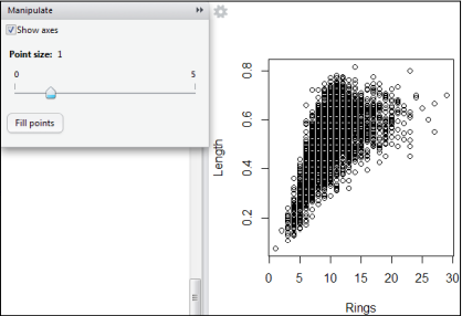
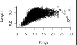
In this example, we are going to create a report of a simple analysis on the Abalone dataset that we’ve used throughout the book. We assume that by now you have an RStudio project directory with a subdirectory data that holds the abalone. cav file. See Chapter 1, Getting Started, to see how to obtain the file (it is also included in the github repository mentioned in the preceding section).

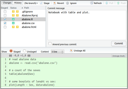
To start, create a new directory named Rmd and a file called density. Rmd. In the example, we are going to estimate the “density” (weight per volume) of abalones, by modeling them as rectangular boxes. We start with a title, author name, and date as follows:

Here, the double-underlining tells Markdown that the text above it should be treated as the document title (in HTML it will be put between the $<\mathrm{H} 1>$ tag as well as between $<$ titles</titles). Under the title, we add the author names, and between brackets, the current date as returned by $R$. This is the first example of inline code. In Markdown, text between single backticks is interpreted and printed as code. By adding an $r$ behind the first backtick, we tell knitr to replace the R code between backticks with its result.
Next, an introducing section is added.

统计代写|R 统计计算作业代写Introduction to Statistical Computing with R代考|R Markdown and Rhtml

统计计算代写

统计代写|R 统计计算作业代写Introduction to Statistical Computing with R代考|Publishing a notebook

Markdown(由 John Gruber 和 Aaron Swartz 创建)是一种易于阅读和易于编写的标记语言,旨在简化 HTML 文档(网页)的准备工作。Markdown 语法的灵感来自人们编写纯文本电子邮件的方式。例如,为了强调电子邮件中的一个词,经常使用*强调词*或_强调词_之类的结构。此外,人们倾向于使用星号或破折号以纯文本形式表示 hullet 列表。 Markdown 的想法是通过将这些结构转换为等效的 HTML 语法(网页),将它们视为实际的标记命令。使用 Markdown,您可以通过更改文本的大小、字体等来更改文本的外观。使用 Markdown 不能做的是更改文档属性,例如页面大小、边距大小等。如果您需要控制这些功能,您可以考虑切换到 LaTeX(在下一节中描述)。或者,可以使用 Max Kuhn 的 odfWeave 包(RStudio 不支持)。
使用 RStudio,您可以使用 . rmd 或 . Rhtm1 文件——在这些文件中,您将 R 输出与 Markdown 或 HTML 结合起来。请注意,RStudio 还支持编辑纯 Markdown (.md) 和 HTML (.html) 文件。

统计代写|R 统计计算作业代写Introduction to Statistical Computing with R代考|Workflow for R Markdown

要使用 R Markdown 创建报告,请打开或开始一个新的 . rmd 文件(文件∣新的∣R降价)。请注意,. Rmd 选项卡有特殊的菜单项。

单击 Knit HTML 按钮(Ctrl + Shift+H 或命令+转移+H) 以创建和打开报告。如果报告已经打开,它将被更新。
作为第一个示例,让我们创建一个新的 . Rmd 文件,清空它,然后输入:
Adding_one and one_gives ‘1+1’
现在点击 Knit HTML 按钮。RStudio 生成一个 HTML 文件并在查看器中打开它。重要的是要意识到这个 HTML 文件是自包含的。也就是说,所有文本和图形都包含在一个文件中,而网页通常依赖许多外部引用来包含图片。主要优点是您可以存储 HTML 文件并通过电子邮件将其作为单个单元发送。
当一个新的 . 创建 Rmd 文件后,RStudio 会打开一个带有入门指南的示例文件。如果单击 Knit HTML 按钮左侧的 MD 按钮,将打开一个帮助文件,其中显示了 Markdown 的一些语法。在右侧,有 Run、Rerun 和 Chunks 按钮。由于这些存在于 Rnw/Sweave 以及 Rmd 和 Rhtml 文件中,因此将在代码块和块选项部分单独讨论它们。

统计代写|R 统计计算作业代写Introduction to Statistical Computing with R代考|An extended example

为了演示 R Markdown 的一些最重要的功能,我们将通过一个广泛的示例逐步进行。在此示例中,我们将了解如何创建文档和章节标题、方程式,如何将代码块内联以及在单独的块中,以及如何添加指向其他文档的链接。我们还将看到代码块选项的第一个示例。您可以在空文件中键入示例,也可以通过单击 Project | 从 github 中提取示例。新 | 版本控制 | Git 并输入 https://github.com/ratudiobook/abalone.git。
另请参阅第 4 章,管理 R 项目的版本控制。或者,您可以将前面的 URL 复制到浏览器并在线阅读代码。
在这个例子中,我们将创建一个对我们在整本书中使用的鲍鱼数据集进行简单分析的报告。我们假设现在您有一个 RStudio 项目目录,其中包含一个包含鲍鱼的子目录 data。cav 文件。请参阅第 1 章,入门,了解如何获取文件(它也包含在上一节中提到的 github 存储库中)。

首先,创建一个名为 Rmd 的新目录和一个名为 density. RMD。在示例中,我们将通过将鲍鱼建模为矩形框来估计鲍鱼的“密度”(每体积重量)。我们从标题、作者姓名和日期开始,如下所示:

在这里,双下划线告诉 Markdown,它上面的文本应该被视为文档标题(在 HTML 中,它将放在<H1>标签以及之间<标题</titles)。在标题下,我们添加作者姓名,并在括号中添加当前日期R. 这是内联代码的第一个示例。在 Markdown 中,单个反引号之间的文本被解释并打印为代码。通过添加一个r在第一个反引号之后,我们告诉 knitr 将反引号之间的 R 代码替换为其结果。
接下来,增加了介绍部分。

统计代写|R 统计计算作业代写Introduction to Statistical Computing with R代考 请认准statistics-lab™

统计代写请认准statistics-lab™. statistics-lab™为您的留学生涯保驾护航。统计代写|python代写代考

随机过程代考

在概率论概念中,随机过程随机变量的集合。 若一随机系统的样本点是随机函数,则称此函数为样本函数,这一随机系统全部样本函数的集合是一个随机过程。 实际应用中,样本函数的一般定义在时间域或者空间域。 随机过程的实例如股票和汇率的波动、语音信号、视频信号、体温的变化,随机运动如布朗运动、随机徘徊等等。

贝叶斯方法代考

贝叶斯统计概念及数据分析表示使用概率陈述回答有关未知参数的研究问题以及统计范式。后验分布包括关于参数的先验分布,和基于观测数据提供关于参数的信息似然模型。根据选择的先验分布和似然模型,后验分布可以解析或近似,例如,马尔科夫链蒙特卡罗 (MCMC) 方法之一。贝叶斯统计概念及数据分析使用后验分布来形成模型参数的各种摘要,包括点估计,如后验平均值、中位数、百分位数和称为可信区间的区间估计。此外,所有关于模型参数的统计检验都可以表示为基于估计后验分布的概率报表。

广义线性模型代考

广义线性模型(GLM)归属统计学领域,是一种应用灵活的线性回归模型。该模型允许因变量的偏差分布有除了正态分布之外的其它分布。

statistics-lab作为专业的留学生服务机构,多年来已为美国、英国、加拿大、澳洲等留学热门地的学生提供专业的学术服务,包括但不限于Essay代写,Assignment代写,Dissertation代写,Report代写,小组作业代写,Proposal代写,Paper代写,Presentation代写,计算机作业代写,论文修改和润色,网课代做,exam代考等等。写作范围涵盖高中,本科,研究生等海外留学全阶段,辐射金融,经济学,会计学,审计学,管理学等全球99%专业科目。写作团队既有专业英语母语作者,也有海外名校硕博留学生,每位写作老师都拥有过硬的语言能力,专业的学科背景和学术写作经验。我们承诺100%原创,100%专业,100%准时,100%满意。

机器学习代写

随着AI的大潮到来,Machine Learning逐渐成为一个新的学习热点。同时与传统CS相比,Machine Learning在其他领域也有着广泛的应用,因此这门学科成为不仅折磨CS专业同学的“小恶魔”,也是折磨生物、化学、统计等其他学科留学生的“大魔王”。学习Machine learning的一大绊脚石在于使用语言众多,跨学科范围广,所以学习起来尤其困难。但是不管你在学习Machine Learning时遇到任何难题,StudyGate专业导师团队都能为你轻松解决。

多元统计分析代考


基础数据: $N$ 个样本, $P$ 个变量数的单样本,组成的横列的数据表
变量定性: 分类和顺序;变量定量:数值
数学公式的角度分为: 因变量与自变量

时间序列分析代写

随机过程,是依赖于参数的一组随机变量的全体,参数通常是时间。 随机变量是随机现象的数量表现,其时间序列是一组按照时间发生先后顺序进行排列的数据点序列。通常一组时间序列的时间间隔为一恒定值(如1秒,5分钟,12小时,7天,1年),因此时间序列可以作为离散时间数据进行分析处理。研究时间序列数据的意义在于现实中,往往需要研究某个事物其随时间发展变化的规律。这就需要通过研究该事物过去发展的历史记录,以得到其自身发展的规律。

回归分析代写

多元回归分析渐进(Multiple Regression Analysis Asymptotics)属于计量经济学领域,主要是一种数学上的统计分析方法,可以分析复杂情况下各影响因素的数学关系,在自然科学、社会和经济学等多个领域内应用广泛。

MATLAB代写

MATLAB 是一种用于技术计算的高性能语言。它将计算、可视化和编程集成在一个易于使用的环境中,其中问题和解决方案以熟悉的数学符号表示。典型用途包括:数学和计算算法开发建模、仿真和原型制作数据分析、探索和可视化科学和工程图形应用程序开发,包括图形用户界面构建MATLAB 是一个交互式系统,其基本数据元素是一个不需要维度的数组。这使您可以解决许多技术计算问题,尤其是那些具有矩阵和向量公式的问题,而只需用 C 或 Fortran 等标量非交互式语言编写程序所需的时间的一小部分。MATLAB 名称代表矩阵实验室。MATLAB 最初的编写目的是提供对由 LINPACK 和 EISPACK 项目开发的矩阵软件的轻松访问,这两个项目共同代表了矩阵计算软件的最新技术。MATLAB 经过多年的发展,得到了许多用户的投入。在大学环境中,它是数学、工程和科学入门和高级课程的标准教学工具。在工业领域,MATLAB 是高效研究、开发和分析的首选工具。MATLAB 具有一系列称为工具箱的特定于应用程序的解决方案。对于大多数 MATLAB 用户来说非常重要,工具箱允许您学习应用专业技术。工具箱是 MATLAB 函数(M 文件)的综合集合,可扩展 MATLAB 环境以解决特定类别的问题。可用工具箱的领域包括信号处理、控制系统、神经网络、模糊逻辑、小波、仿真等。

R语言代写问卷设计与分析代写
PYTHON代写回归分析与线性模型代写
MATLAB代写方差分析与试验设计代写
STATA代写机器学习/统计学习代写
SPSS代写计量经济学代写
EVIEWS代写时间序列分析代写
EXCEL代写深度学习代写
SQL代写各种数据建模与可视化代写

统计代写|R 统计计算作业代写Introduction to Statistical Computing with R代考|Generating Reports

如果你也在 怎样代写R 统计计算Introduction to Statistical Computing with R这个学科遇到相关的难题,请随时右上角联系我们的24/7代写客服。

R 统计计算和统计计算是采用计算、图形和数字方法解决统计问题的两个领域,这使得多功能的R语言成为这些领域的理想计算环境。

statistics-lab™ 为您的留学生涯保驾护航 在代写R 统计计算Introduction to Statistical Computing with R方面已经树立了自己的口碑, 保证靠谱, 高质且原创的统计Statistics代写服务。我们的专家在代写R 统计计算方面经验极为丰富,各种代写R 统计计算Introduction to Statistical Computing with R相关的作业也就用不着说。

我们提供的R 统计计算Introduction to Statistical Computing with R代写及其相关学科的代写,服务范围广, 其中包括但不限于:

  • Statistical Inference 统计推断
  • Statistical Computing 统计计算
  • Advanced Probability Theory 高等楖率论
  • Advanced Mathematical Statistics 高等数理统计学
  • (Generalized) Linear Models 广义线性模型
  • Statistical Machine Learning 统计机器学习
  • Longitudinal Data Analysis 纵向数据分析
  • Foundations of Data Science 数据科学基础
统计代写|R 统计计算作业代写Introduction to Statistical Computing with R代考|Generating Reports

统计代写|R 统计计算作业代写Introduction to Statistical Computing with R代考|Generating Reports

In this chapter, we treat three different ways to produce reports that automatically include the results of an analysis.

A very important feature of reproducible science is generating reports. The main idea of automatic report generation is that the results of analyses are not manually copied to the report. Instead, both the $R$ code and the report’s text are combined in one or more plain text files. The report is generated by a tool that executes the chunks of code, captures the results (including figures), and generates the report by weaving the report’s text and results together. To achieve this, you need to learn a few special commands, called markup specifiers, that tell the report generator which part of your text is $\mathrm{R}$ code, and which parts you want in special typesetting such as boldface or italic. There are several markup languages to do this, but the following is a minimal example using the Markdown language:

The left panel shows the plain text file in RStudio’s editor and the right panel shows the web page that is generated by clicking on the Knit HTML button. The markup specifiers used here are the double asterisks for boldface, single underscores for slanted font, and the backticks for code. By adding an $x$ to the first backtick, the report generator executes the code following it.

The Markdown language is one of many markup languages in existence and RStudio supports several of them. RStudio has excellent support for interweaving code with Markdown, HTML, LaTeX, or even in plain comments. We’ve encountered the latter option already in Chapter 1, Getting Started, when we created a notebook straight from R script.

Notebooks are useful to quickly share annotated lines of code or results. There are a few ways to control the layout of a notebook. The Markdown language is easy to learn and has a fair amount of layout options. It also allows you to include equations in the LaTeX format. The HTML option is really only useful if you aim to create a web page. You should know, or be willing to learn HTML to use it. The result of these three methods is always a web page (that is, an HTML file) although this can be exported to PDF.
If you need ultimate control over your document’s layout, and if you need features like automated bibliographies and equation numbering, LaTeX is the way to go. With this last option, it is possible to create papers for scientific journals straight from your analysis.

Depending on the chosen system, a text file with a different extension is used as the source file. The following table gives an overview.

Finally, we note that the interweaving of code and text (often referred to as literate programming) may serve two purposes. The first, described in this chapter, is to gencrate a data analysis report by cxccuting code to produce the result. The second is to document the code itself, for example, by describing the purpose of a function and all its arguments. The latter purpose will be discussed in the next chapter, where we will discuss the Roxygen2 package for code documentation.

统计代写|R 统计计算作业代写Introduction to Statistical Computing with R代考|Prerequisites for report generation

For notebooks, R Markdown, and Rhtml, RStudio relies on Yihui Xie’s knitr package for executing code chunks and merging the results. The knitr package can be installed via RStudio’s Packages tab or with the command install. packages (“knitr”).

For LaTeX/Sweave files, the default is to use R’s native Sweave driver. The knitr package is easier to use and has more options for fine-tuning, so in the rest of this chapter we assume that knitr is always used. To make sure that knitr is also used for Sweave files, go to Tools | Options | Sweave and choose knitr as Weave Rnw files. If you’re working in an RStudio project, you can set this as a project option as well by navigating to Project | Project Options | Sweave. When you work with LaTeX/Sweave, you need to have a working LaTeX distribution installed. Popular distributions are TeXLive for Linux, MikTeX for Windows, and MacTeX for Mac OS X.

统计代写|R 统计计算作业代写Introduction to Statistical Computing with R代考|Notebook options

RStudio offers three ways to generate a notebook from an Rscript – the simplest are Default and knitr:istitch. These only differ a little in layout. The knitr:spin mode allows you to use the Markdown markup language to specify text layout. The markup options are presented after navigating to File | Notebook or after clicking on the Notebook button. Under the hood, the Default and knitr::stitch options use knitr to generate a Markdown file which is then directly converted to a web page (HTML file). The knitr:spin mode allows for using Markdown commands in your comments and will convert your . R file to a .Rmd (R Markdown) file before further processing.

In Default mode, $R$ code and printed results are rendered to code blocks in a fixedwidth font with a different background color. Figures are included in the output and the document is prepended with a title, an optional author name, and the date. The only option to include text in your output is to add it as an R comment (behind the # sign) and it will be rendered as such.
In knitr:stitch mode, instead of prepending the report with an author name and date, the report is appended with a call to Sys . time () and R’s sessionInfo(). The latter is useful since it shows the context in which the code was executed including R’s version, locale settings, and loaded packages. The result of the knitr::stitch mode depends on a template file called knitr-template. Rnw, included with the knitr package. It is stored in a directory that you can find by typing system.
file (‘misc’, package=’ knitr’).

统计代写|R 统计计算作业代写Introduction to Statistical Computing with R代考|Generating Reports

统计计算代写

统计代写|R 统计计算作业代写Introduction to Statistical Computing with R代考|Generating Reports

在本章中,我们将介绍生成自动包含分析结果的报告的三种不同方法。

可重复科学的一个非常重要的特征是生成报告。自动报告生成的主要思想是分析结果不会手动复制到报告中。相反,两者R代码和报告的文本合并在一个或多个纯文本文件中。报告由执行代码块、捕获结果(包括数字)并通过将报告的文本和结果编织在一起来生成报告的工具生成。为此,您需要学习一些称为标记说明符的特殊命令,它们告诉报告生成器您的文本的哪一部分是R代码,以及您想要特殊排版的部分,例如粗体或斜体。有几种标记语言可以做到这一点,但以下是使用 Markdown 语言的最小示例:

左侧面板显示 RStudio 编辑器中的纯文本文件,右侧面板显示通过单击 Knit HTML 按钮生成的网页。这里使用的标记说明符是粗体的双星号、倾斜字体的单下划线和代码的反引号。通过添加一个X对于第一个反引号,报告生成器执行它后面的代码。

Markdown 语言是现有的许多标记语言之一,RStudio 支持其中的几种。RStudio 非常支持将代码与 Markdown、HTML、LaTeX 甚至是纯注释交织在一起。我们已经在第 1 章“入门”中遇到过后一种选择,当时我们直接从 R 脚本创建了一个笔记本。

笔记本对于快速共享带注释的代码行或结果很有用。有几种方法可以控制笔记本的布局。Markdown 语言易于学习,并且有大量的布局选项。它还允许您以 LaTeX 格式包含方程式。只有当您的目标是创建网页时,HTML 选项才真正有用。您应该知道或愿意学习 HTML 以使用它。这三种方法的结果始终是一个网页(即 HTML 文件),尽管可以将其导出为 PDF。
如果您需要对文档的布局进行最终控制,并且需要自动参考书目和方程式编号等功能,那么 LaTeX 就是您的最佳选择。使用最后一个选项,可以直接根据您的分析为科学期刊创建论文。

根据所选系统,将使用具有不同扩展名的文本文件作为源文件。下表给出了概述。

最后,我们注意到代码和文本的交织(通常称为文学编程)可能有两个目的。本章描述的第一个是通过编写代码生成数据分析报告以产生结果。第二个是记录代码本身,例如,通过描述函数的用途及其所有参数。后一个目的将在下一章讨论,我们将在其中讨论用于代码文档的 Roxygen2 包。

统计代写|R 统计计算作业代写Introduction to Statistical Computing with R代考|Prerequisites for report generation

对于 notebook、R Markdown 和 Rhtml,RStudio 依赖于 Yihui Xie 的 knitr 包来执行代码块并合并结果。knitr 包可以通过 RStudio 的 Packages 选项卡或使用命令 install 安装。包(“knitr”)。

对于 LaTeX/Sweave 文件,默认使用 R 的原生 Sweave 驱动程序。knitr 包更容易使用并且有更多的微调选项,所以在本章的其余部分我们假设总是使用 knitr。要确保 knitr 也用于 Sweave 文件,请转到工具 | 选项 | Sweave 并选择 knitr 作为 Weave Rnw 文件。如果您在 RStudio 项目中工作,您也可以通过导航到 Project | 将其设置为项目选项。项目选项 | 编织。当你使用 LaTeX/Sweave 时,你需要安装一个工作的 LaTeX 发行版。流行的发行版是 Linux 的 TeXLive、Windows 的 MikTeX 和 Mac OS X 的 MacTeX。

统计代写|R 统计计算作业代写Introduction to Statistical Computing with R代考|Notebook options

RStudio 提供了三种从 Rscript 生成笔记本的方法——最简单的是 Default 和 knitr:istitch。这些只是布局略有不同。knitr:spin 模式允许您使用 Markdown 标记语言来指定文本布局。导航到 File | 后会显示标记选项。笔记本或单击笔记本按钮后。在后台, Default 和 knitr::stitch 选项使用 knitr 生成 Markdown 文件,然后直接将其转换为网页(HTML 文件)。knitr:spin 模式允许在您的评论中使用 Markdown 命令,并将转换您的 . 在进一步处理之前将 R 文件转换为 .Rmd (R Markdown) 文件。

在默认模式下,R代码和打印结果以具有不同背景颜色的固定宽度字体呈现给代码块。图片包含在输出中,文档前面有标题、可选的作者姓名和日期。在输出中包含文本的唯一选择是将其添加为 R 注释(在 # 符号后面),它将按原样呈现。
在 knitr:stitch 模式下,不是在报告前面加上作者姓名和日期,而是在报告后面附加对 Sys 的调用。time() 和 R 的 sessionInfo()。后者很有用,因为它显示了执行代码的上下文,包括 R 的版本、区域设置和加载的包。knitr::stitch 模式的结果取决于名为 knitr-template 的模板文件。Rnw,包含在 knitr 包中。它存储在一个目录中,您可以通过键入系统找到该目录。
文件(’misc’,package=’knitr’)。

统计代写|R 统计计算作业代写Introduction to Statistical Computing with R代考 请认准statistics-lab™

统计代写请认准statistics-lab™. statistics-lab™为您的留学生涯保驾护航。统计代写|python代写代考

随机过程代考

在概率论概念中,随机过程随机变量的集合。 若一随机系统的样本点是随机函数,则称此函数为样本函数,这一随机系统全部样本函数的集合是一个随机过程。 实际应用中,样本函数的一般定义在时间域或者空间域。 随机过程的实例如股票和汇率的波动、语音信号、视频信号、体温的变化,随机运动如布朗运动、随机徘徊等等。

贝叶斯方法代考

贝叶斯统计概念及数据分析表示使用概率陈述回答有关未知参数的研究问题以及统计范式。后验分布包括关于参数的先验分布,和基于观测数据提供关于参数的信息似然模型。根据选择的先验分布和似然模型,后验分布可以解析或近似,例如,马尔科夫链蒙特卡罗 (MCMC) 方法之一。贝叶斯统计概念及数据分析使用后验分布来形成模型参数的各种摘要,包括点估计,如后验平均值、中位数、百分位数和称为可信区间的区间估计。此外,所有关于模型参数的统计检验都可以表示为基于估计后验分布的概率报表。

广义线性模型代考

广义线性模型(GLM)归属统计学领域,是一种应用灵活的线性回归模型。该模型允许因变量的偏差分布有除了正态分布之外的其它分布。

statistics-lab作为专业的留学生服务机构,多年来已为美国、英国、加拿大、澳洲等留学热门地的学生提供专业的学术服务,包括但不限于Essay代写,Assignment代写,Dissertation代写,Report代写,小组作业代写,Proposal代写,Paper代写,Presentation代写,计算机作业代写,论文修改和润色,网课代做,exam代考等等。写作范围涵盖高中,本科,研究生等海外留学全阶段,辐射金融,经济学,会计学,审计学,管理学等全球99%专业科目。写作团队既有专业英语母语作者,也有海外名校硕博留学生,每位写作老师都拥有过硬的语言能力,专业的学科背景和学术写作经验。我们承诺100%原创,100%专业,100%准时,100%满意。

机器学习代写

随着AI的大潮到来,Machine Learning逐渐成为一个新的学习热点。同时与传统CS相比,Machine Learning在其他领域也有着广泛的应用,因此这门学科成为不仅折磨CS专业同学的“小恶魔”,也是折磨生物、化学、统计等其他学科留学生的“大魔王”。学习Machine learning的一大绊脚石在于使用语言众多,跨学科范围广,所以学习起来尤其困难。但是不管你在学习Machine Learning时遇到任何难题,StudyGate专业导师团队都能为你轻松解决。

多元统计分析代考


基础数据: $N$ 个样本, $P$ 个变量数的单样本,组成的横列的数据表
变量定性: 分类和顺序;变量定量:数值
数学公式的角度分为: 因变量与自变量

时间序列分析代写

随机过程,是依赖于参数的一组随机变量的全体,参数通常是时间。 随机变量是随机现象的数量表现,其时间序列是一组按照时间发生先后顺序进行排列的数据点序列。通常一组时间序列的时间间隔为一恒定值(如1秒,5分钟,12小时,7天,1年),因此时间序列可以作为离散时间数据进行分析处理。研究时间序列数据的意义在于现实中,往往需要研究某个事物其随时间发展变化的规律。这就需要通过研究该事物过去发展的历史记录,以得到其自身发展的规律。

回归分析代写

多元回归分析渐进(Multiple Regression Analysis Asymptotics)属于计量经济学领域,主要是一种数学上的统计分析方法,可以分析复杂情况下各影响因素的数学关系,在自然科学、社会和经济学等多个领域内应用广泛。

MATLAB代写

MATLAB 是一种用于技术计算的高性能语言。它将计算、可视化和编程集成在一个易于使用的环境中,其中问题和解决方案以熟悉的数学符号表示。典型用途包括:数学和计算算法开发建模、仿真和原型制作数据分析、探索和可视化科学和工程图形应用程序开发,包括图形用户界面构建MATLAB 是一个交互式系统,其基本数据元素是一个不需要维度的数组。这使您可以解决许多技术计算问题,尤其是那些具有矩阵和向量公式的问题,而只需用 C 或 Fortran 等标量非交互式语言编写程序所需的时间的一小部分。MATLAB 名称代表矩阵实验室。MATLAB 最初的编写目的是提供对由 LINPACK 和 EISPACK 项目开发的矩阵软件的轻松访问,这两个项目共同代表了矩阵计算软件的最新技术。MATLAB 经过多年的发展,得到了许多用户的投入。在大学环境中,它是数学、工程和科学入门和高级课程的标准教学工具。在工业领域,MATLAB 是高效研究、开发和分析的首选工具。MATLAB 具有一系列称为工具箱的特定于应用程序的解决方案。对于大多数 MATLAB 用户来说非常重要,工具箱允许您学习应用专业技术。工具箱是 MATLAB 函数(M 文件)的综合集合,可扩展 MATLAB 环境以解决特定类别的问题。可用工具箱的领域包括信号处理、控制系统、神经网络、模糊逻辑、小波、仿真等。

R语言代写问卷设计与分析代写
PYTHON代写回归分析与线性模型代写
MATLAB代写方差分析与试验设计代写
STATA代写机器学习/统计学习代写
SPSS代写计量经济学代写
EVIEWS代写时间序列分析代写
EXCEL代写深度学习代写
SQL代写各种数据建模与可视化代写

统计代写|R 统计计算作业代写Introduction to Statistical Computing with R代考|Subversion

如果你也在 怎样代写R 统计计算Introduction to Statistical Computing with R这个学科遇到相关的难题,请随时右上角联系我们的24/7代写客服。

R 统计计算和统计计算是采用计算、图形和数字方法解决统计问题的两个领域,这使得多功能的R语言成为这些领域的理想计算环境。

statistics-lab™ 为您的留学生涯保驾护航 在代写R 统计计算Introduction to Statistical Computing with R方面已经树立了自己的口碑, 保证靠谱, 高质且原创的统计Statistics代写服务。我们的专家在代写R 统计计算方面经验极为丰富,各种代写R 统计计算Introduction to Statistical Computing with R相关的作业也就用不着说。

我们提供的R 统计计算Introduction to Statistical Computing with R代写及其相关学科的代写,服务范围广, 其中包括但不限于:

  • Statistical Inference 统计推断
  • Statistical Computing 统计计算
  • Advanced Probability Theory 高等楖率论
  • Advanced Mathematical Statistics 高等数理统计学
  • (Generalized) Linear Models 广义线性模型
  • Statistical Machine Learning 统计机器学习
  • Longitudinal Data Analysis 纵向数据分析
  • Foundations of Data Science 数据科学基础
统计代写|R 统计计算作业代写Introduction to Statistical Computing with R代考|Subversion

统计代写|R 统计计算作业代写Introduction to Statistical Computing with R代考|Create a new

In Subversion, the location of the repository that stores increments of your project is different from the directory where you actually do your work. To create a project under Subversion version control, perform the following steps:

  1. Create a new svn repository.
    In your operating system’s command-line interface, you can do this by typing svnadmin create epath to projectnames. A new directory will be created with some svn-specific files. You should never alter this directory yourself. It is where Subversion will store incremental versions of your project.
  2. In some directory, for example, in /projects/, do an svn checkout. In your operating system’s command-line interface, you can do this by typing svn checkout file:/// (notice the triple slash after file:).
  3. Open RStudio. Go to Project | Create project… | Existing directory. Choose the directory that you just checked out from the empty Subversion repository.
  4. Or, instead of the last two steps, you can go to Project | Create project | Version Control | Subversion. Type file: $/ / /<$ path to projectname> in Repository Url and RStudio will do the rest for you.
  5. We made a fresh empty repository named abalone, checked it out with Subversion, and created an RStudio project in the checked-out directory. The RStudio panel now contains an extra tab SVN, shown in the following screenshot. We will replay some of the steps of the previous section, but now with Subversion.

The yellow question mark shows that abalone. Rproj is not (yet) in the central repository.
The SVN tab of RStudio has a Status column containing icons that indicate the status of files with respect to their versions in the central repository. At the moment, there is only the abalone. Rproj file, which has not been added to the repository yet, so it is marked with a question mark icon. An overview of SVN status icons is given in the following table.

统计代写|R 统计计算作业代写Introduction to Statistical Computing with R代考|Working with a team

Working with a team on a project is almost unthinkable without a version control system. In principle, with GIT it is possible to work without a central repository. However, it is very common to still work with a central repository where collaborators can pull changes from and push their own. There are several online resources where you can host your open source projects free of charge. Popular ones include github (obviously supporting GTT only), code. google. com, and bitbucket. The latter two support GIT as well as Subversion. At the time of writing, bitbucket is the only of these three hosting non-open repositories for free as well.

To start on a project with an online repository, you need to create an account and create a new project at the hosting site. When you create a project, you usually have to choose the version control system you want to use. Once the online repository is created, start RStudio and click on Project | New project. Choose Check out a project from a version control repository. After choosing the version control system, you will be asked for the URL of your repository and where to store the files on your own computer.

Now, for GIT repositories, the workflow is as follows. To get the updates from your collaborators, pull the latest changes via the Git tab menu More | Pull Branches. Next, you can do the work, stage files, and commit them with a comment. After the commit, the local copy of the GIT repository is updated. However, to send the same changes to your coworkers, you need to push the latest commits to the central repository via More | Push Branch.
For subversion repositories, you need to update your working copy, using More | Update. After the work is done, when you commit the changes, they will be immediately uploaded to the central repository.

统计代写|R 统计计算作业代写Introduction to Statistical Computing with R代考|Further reading

There is much more to be said about version control and we have only covered enough here to get you started with the most common operations. As you grow accustomed with version control, you probably want to start using more features than are currently interfaced through RStudio. The first features to look into are probably branching and merging of development lines and reverting commits. A good online resource for using GIT on the command line is the GIT book (http://git-scm. com/book). For Subversion, the SVN book (http: // avnbook . red-bean . com), which is partly written by some of Subversion’s developers comes highly recommended. Both books can be read for free online or ordered as a hard copy.

统计代写|R 统计计算作业代写Introduction to Statistical Computing with R代考|Subversion

统计计算代写

统计代写|R 统计计算作业代写Introduction to Statistical Computing with R代考|Create a new

在 Subversion 中,存储项目增量的存储库的位置与您实际工作的目录不同。要在 Subversion 版本控制下创建项目,请执行以下步骤:

  1. 创建一个新的 svn 存储库。
    在您的操作系统的命令行界面中,您可以通过键入 svnadmin create epath to projectnames 来执行此操作。将使用一些特定于 svn 的文件创建一个新目录。你不应该自己改变这个目录。Subversion 将在这里存储项目的增量版本。
  2. 在某个目录中,例如,在 /projects/ 中,执行 svn checkout。在您的操作系统的命令行界面中,您可以通过键入 svn checkout file:/// 来执行此操作(注意 file: 后面的三个斜杠)。
  3. 打开 RStudio。前往项目 | 创建项目… | 现有目录。从空的 Subversion 存储库中选择您刚刚签出的目录。
  4. 或者,代替最后两个步骤,您可以转到项目 | 创建项目 | 版本控制 | 颠覆。类型文件:///<存储库 URL 中 projectname> 的路径,RStudio 将为您完成剩下的工作。
  5. 我们新建了一个名为 abalone 的空存储库,使用 Subversion 将其签出,并在签出目录中创建了一个 RStudio 项目。RStudio 面板现在包含一个额外的选项卡 SVN,如以下屏幕截图所示。我们将重播上一节的一些步骤,但现在使用 Subversion。

黄色问号表示鲍鱼。Rproj (尚未)在中央存储库中。
RStudio 的 SVN 选项卡有一个 Status 列,其中包含指示文件相对于中央存储库中的版本的状态的图标。此刻,只有鲍鱼。rproj 文件,该文件尚未添加到存储库中,因此标有问号图标。下表给出了 SVN 状态图标的概述。

统计代写|R 统计计算作业代写Introduction to Statistical Computing with R代考|Working with a team

如果没有版本控制系统,几乎无法想象在一个项目上与团队合作。原则上,使用 GIT 可以在没有中央存储库的情况下工作。但是,仍然使用中央存储库是很常见的,协作者可以从中提取更改并推送自己的更改。您可以通过多种在线资源免费托管您的开源项目。流行的包括github(显然只支持GTT),代码。谷歌。com 和 bitbucket。后两者支持 GIT 和 Subversion。在撰写本文时,bitbucket 也是这三个免费托管的非开放存储库中唯一的一个。

要开始使用在线存储库的项目,您需要创建一个帐户并在托管站点上创建一个新项目。创建项目时,通常必须选择要使用的版本控制系统。创建在线存储库后,启动 RStudio 并单击 Project | 新项目。选择从版本控制存储库中签出项目。选择版本控制系统后,系统会询问您存储库的 URL 以及在您自己的计算机上存储文件的位置。

现在,对于 GIT 存储库,工作流程如下。要从您的协作者那里获取更新,请通过 Git 选项卡菜单获取最新更改 更多 | 拉树枝。接下来,您可以完成工作、暂存文件并使用评论提交它们。提交后,GIT 存储库的本地副本被更新。但是,要将相同的更改发送给您的同事,您需要通过更多 | 将最新提交推送到中央存储库。推送分支。
对于 subversion 存储库,您需要使用更多 | 更新您的工作副本。更新。工作完成后,当您提交更改时,它们将立即上传到中央存储库。

统计代写|R 统计计算作业代写Introduction to Statistical Computing with R代考|Further reading

关于版本控制还有很多话要说,我们在这里只介绍了足够的内容来帮助您开始最常见的操作。随着您逐渐习惯了版本控制,您可能希望开始使用比目前通过 RStudio 接口更多的功能。首先要研究的功能可能是开发线的分支和合并以及恢复提交。在命令行上使用 GIT 的一个很好的在线资源是 GIT book (http://git-scm.com/book)。对于 Subversion,强烈推荐部分由部分 Subversion 开发人员编写的 SVN 书籍 (http://avnbook.red-bean.com)。这两本书都可以在线免费阅读或以硬拷贝的形式订购。

统计代写|R 统计计算作业代写Introduction to Statistical Computing with R代考 请认准statistics-lab™

统计代写请认准statistics-lab™. statistics-lab™为您的留学生涯保驾护航。统计代写|python代写代考

随机过程代考

在概率论概念中,随机过程随机变量的集合。 若一随机系统的样本点是随机函数,则称此函数为样本函数,这一随机系统全部样本函数的集合是一个随机过程。 实际应用中,样本函数的一般定义在时间域或者空间域。 随机过程的实例如股票和汇率的波动、语音信号、视频信号、体温的变化,随机运动如布朗运动、随机徘徊等等。

贝叶斯方法代考

贝叶斯统计概念及数据分析表示使用概率陈述回答有关未知参数的研究问题以及统计范式。后验分布包括关于参数的先验分布,和基于观测数据提供关于参数的信息似然模型。根据选择的先验分布和似然模型,后验分布可以解析或近似,例如,马尔科夫链蒙特卡罗 (MCMC) 方法之一。贝叶斯统计概念及数据分析使用后验分布来形成模型参数的各种摘要,包括点估计,如后验平均值、中位数、百分位数和称为可信区间的区间估计。此外,所有关于模型参数的统计检验都可以表示为基于估计后验分布的概率报表。

广义线性模型代考

广义线性模型(GLM)归属统计学领域,是一种应用灵活的线性回归模型。该模型允许因变量的偏差分布有除了正态分布之外的其它分布。

statistics-lab作为专业的留学生服务机构,多年来已为美国、英国、加拿大、澳洲等留学热门地的学生提供专业的学术服务,包括但不限于Essay代写,Assignment代写,Dissertation代写,Report代写,小组作业代写,Proposal代写,Paper代写,Presentation代写,计算机作业代写,论文修改和润色,网课代做,exam代考等等。写作范围涵盖高中,本科,研究生等海外留学全阶段,辐射金融,经济学,会计学,审计学,管理学等全球99%专业科目。写作团队既有专业英语母语作者,也有海外名校硕博留学生,每位写作老师都拥有过硬的语言能力,专业的学科背景和学术写作经验。我们承诺100%原创,100%专业,100%准时,100%满意。

机器学习代写

随着AI的大潮到来,Machine Learning逐渐成为一个新的学习热点。同时与传统CS相比,Machine Learning在其他领域也有着广泛的应用,因此这门学科成为不仅折磨CS专业同学的“小恶魔”,也是折磨生物、化学、统计等其他学科留学生的“大魔王”。学习Machine learning的一大绊脚石在于使用语言众多,跨学科范围广,所以学习起来尤其困难。但是不管你在学习Machine Learning时遇到任何难题,StudyGate专业导师团队都能为你轻松解决。

多元统计分析代考


基础数据: $N$ 个样本, $P$ 个变量数的单样本,组成的横列的数据表
变量定性: 分类和顺序;变量定量:数值
数学公式的角度分为: 因变量与自变量

时间序列分析代写

随机过程,是依赖于参数的一组随机变量的全体,参数通常是时间。 随机变量是随机现象的数量表现,其时间序列是一组按照时间发生先后顺序进行排列的数据点序列。通常一组时间序列的时间间隔为一恒定值(如1秒,5分钟,12小时,7天,1年),因此时间序列可以作为离散时间数据进行分析处理。研究时间序列数据的意义在于现实中,往往需要研究某个事物其随时间发展变化的规律。这就需要通过研究该事物过去发展的历史记录,以得到其自身发展的规律。

回归分析代写

多元回归分析渐进(Multiple Regression Analysis Asymptotics)属于计量经济学领域,主要是一种数学上的统计分析方法,可以分析复杂情况下各影响因素的数学关系,在自然科学、社会和经济学等多个领域内应用广泛。

MATLAB代写

MATLAB 是一种用于技术计算的高性能语言。它将计算、可视化和编程集成在一个易于使用的环境中,其中问题和解决方案以熟悉的数学符号表示。典型用途包括:数学和计算算法开发建模、仿真和原型制作数据分析、探索和可视化科学和工程图形应用程序开发,包括图形用户界面构建MATLAB 是一个交互式系统,其基本数据元素是一个不需要维度的数组。这使您可以解决许多技术计算问题,尤其是那些具有矩阵和向量公式的问题,而只需用 C 或 Fortran 等标量非交互式语言编写程序所需的时间的一小部分。MATLAB 名称代表矩阵实验室。MATLAB 最初的编写目的是提供对由 LINPACK 和 EISPACK 项目开发的矩阵软件的轻松访问,这两个项目共同代表了矩阵计算软件的最新技术。MATLAB 经过多年的发展,得到了许多用户的投入。在大学环境中,它是数学、工程和科学入门和高级课程的标准教学工具。在工业领域,MATLAB 是高效研究、开发和分析的首选工具。MATLAB 具有一系列称为工具箱的特定于应用程序的解决方案。对于大多数 MATLAB 用户来说非常重要,工具箱允许您学习应用专业技术。工具箱是 MATLAB 函数(M 文件)的综合集合,可扩展 MATLAB 环境以解决特定类别的问题。可用工具箱的领域包括信号处理、控制系统、神经网络、模糊逻辑、小波、仿真等。

R语言代写问卷设计与分析代写
PYTHON代写回归分析与线性模型代写
MATLAB代写方差分析与试验设计代写
STATA代写机器学习/统计学习代写
SPSS代写计量经济学代写
EVIEWS代写时间序列分析代写
EXCEL代写深度学习代写
SQL代写各种数据建模与可视化代写

统计代写|R 统计计算作业代写Introduction to Statistical Computing with R代考|Version control

如果你也在 怎样代写R 统计计算Introduction to Statistical Computing with R这个学科遇到相关的难题,请随时右上角联系我们的24/7代写客服。

R 统计计算和统计计算是采用计算、图形和数字方法解决统计问题的两个领域,这使得多功能的R语言成为这些领域的理想计算环境。

statistics-lab™ 为您的留学生涯保驾护航 在代写R 统计计算Introduction to Statistical Computing with R方面已经树立了自己的口碑, 保证靠谱, 高质且原创的统计Statistics代写服务。我们的专家在代写R 统计计算方面经验极为丰富,各种代写R 统计计算Introduction to Statistical Computing with R相关的作业也就用不着说。

我们提供的R 统计计算Introduction to Statistical Computing with R代写及其相关学科的代写,服务范围广, 其中包括但不限于:

  • Statistical Inference 统计推断
  • Statistical Computing 统计计算
  • Advanced Probability Theory 高等楖率论
  • Advanced Mathematical Statistics 高等数理统计学
  • (Generalized) Linear Models 广义线性模型
  • Statistical Machine Learning 统计机器学习
  • Longitudinal Data Analysis 纵向数据分析
  • Foundations of Data Science 数据科学基础

统计代写|R 统计计算作业代写Introduction to Statistical Computing with R代考|Installing GIT or Subversion

You need to have GIT and/or Subversion installed to be able to use them from RStudio. Both are frec and open source tools. Most Linux distributions include a version of GIT and Subversion in their application repositories. For example, under Debian-based distributions such as Ubuntu, open a terminal and type the following statements to install GIT or Subversion:
sudo apt-get install git-core
sudo apt-get install subversion
Alternatively, use Synaptic or another graphical package manager to install it. For Windows, the authors of RStudio recommend msysGit (ht tp://msysgit. github. com/) as the GIT client and SlikSVN for Subversion. The popular TortoiseSVN (tortoisesvn. net) is not supported by RStudio since it does not offer a command-line interface that RStudio uses to control the version control system. You can use TortoiseSVN alongside RStudio with no problems, however. For OS X, you can use GIT-osx-installer available at http://code . google. $\mathrm{com} / \mathrm{p} / \mathrm{git}$-osx-installer. For OS X version $10.7$ and lower, a Subversion client is already installed. For $10.8$ and higher, you need to install Xcode and download the command-line tools via Xcode Preferences.

统计代写|R 统计计算作业代写Introduction to Statistical Computing with R代考|Version control for single-person projects

Although it may at first not be obvious, using a version control system for your own work has its merits. Once you grow accustomed to managing $R$ projects with source control, you’ll find it hard to believe how you managed without it. In the following sections, we will demonstrate a simple example, first using GIT and next using Subversion as version control system.

To demonstrate how to work with a local version control repository, we will work through some examples of our Abalone project. If you don’t have those files (anymore), you can download or view them at ht tps://github.com/ rstudiobook/abalone. When we left the project in Chapter 1, Getting Started, we had the following files:

If you set the project up with the Create a git repository for the project option checked, there should be a Git tab near your workspace browser. If not, you can still create one now by going to Project | Project options | Version control and choosing Git as the version control system from the drop-down ment

Once a repository has been created, working with GIT has the following basic workflow:

  1. If necessary, get the latest version of the project from the repository (pull). This is only necessary when collaborating with multiple developers.
  2. Do the work – create, delete, move, or alter files.
  3. Stage changes you want to commit to the repository. That is, you need to tell GIT which of the alterations should make it to the repository.
  4. Commit the staged changes to the repository.

统计代写|R 统计计算作业代写Introduction to Statistical Computing with R代考|Existing directory

The staging part of the workflow is an important feature that sets GIT apart from Subversion. Staging gives you the freedom to try quick and dirty stuff that you may not want to end up in the repository. It saves you making the famous <filenames. 1 copy, since none of the changes will be submitted as long as you don’t stage them. Reverting work that has been staged, but not committed, can be done with the click of a button in RStudio and will be discussed next.

Thus far in our Abalone example, we have only created a repository for GIT. Nothing has been committed to that repository yet, and we first need to decide which files we want to bring under version control. The only files that are directly created by us are abalone. cav and abalone. R. The abalone. htmi file was generated automatically from our R script when we compiled the notebook. Since this is the output of our script, we do not need to put it under version control. It can be recreated any time we want. The files . gitignore and . Rhistory are for GIT and RStudio’s internal use and do not need to be put under version control right now. In some cases, for example, when working with multiple people on a project, it can still be convenient to bring the . gitignore file under version control.

To add files to the version control system, open the Git tab, near the Workspace panel, and mark abalone.R and abalone.csv as shown in the following screenshot:By marking these files, we tell GIT that the files are staged for submission to the repository. This is indicated by the status icons between the checkmarks and the filenames The Status column has two columns of icons The right column is used to indicate that GIT has noticed that a file has been changed since its last commit. A question mark means that the file has not been added to version control yet. When you stage a file, the left icon indicates what the committing action will be. In the preceding screenshot, the A stands for adding. The following table lists the icon combinations used in GIT’s Status column.

统计计算代写

统计代写|R 统计计算作业代写Introduction to Statistical Computing with R代考|Installing GIT or Subversion

您需要安装 GIT 和/或 Subversion 才能从 RStudio 使用它们。两者都是 frec 和开源工具。大多数 Linux 发行版在其应用程序存储库中都包含一个 GIT 和 Subversion 版本。例如,在 Ubuntu 等基于 Debian 的发行版下,打开终端并键入以下语句以安装 GIT 或 Subversion:
sudo apt-get install git-core
sudo apt-get install subversion
或者,使用 Synaptic 或其他图形包管理器来安装它。对于 Windows,RStudio 的作者推荐 msysGit (ht tp://msysgit.github.com/) 作为 GIT 客户端,SlikSVN 作为 Subversion。RStudio 不支持流行的 TortoiseSVN (tortoisesvn.net),因为它不提供 RStudio 用来控制版本控制系统的命令行界面。但是,您可以毫无问题地将 TortoiseSVN 与 RStudio 一起使用。对于 OS X,您可以使用 http://code 上提供的 GIT-osx-installer。谷歌。C这米/p/G一世吨-osx 安装程序。对于 OS X 版本10.7及更低版本,已经安装了 Subversion 客户端。为了10.8及更高版本,您需要安装 Xcode 并通过 Xcode Preferences 下载命令行工具。

统计代写|R 统计计算作业代写Introduction to Statistical Computing with R代考|Version control for single-person projects

虽然一开始可能并不明显,但为自己的工作使用版本控制系统有其优点。一旦你习惯了管理R带有源代码控制的项目,你会很难相信没有它你是如何管理的。在接下来的部分中,我们将演示一个简单的示例,首先使用 GIT,然后使用 Subversion 作为版本控制系统。

为了演示如何使用本地版本控制存储库,我们将通过我们 Aba​​lone 项目的一些示例进行操作。如果您没有这些文件(不再有),您可以在 ht tps://github.com/rstudiobook/abalone 下载或查看它们。当我们在第 1 章“入门”中离开项目时,我们有以下文件:

如果您在选中为项目创建 git 存储库选项设置项目时,您的工作区浏览器附近应该有一个 Git 选项卡。如果没有,您现在仍然可以通过转到 Project | 创建一个。项目选项 | 版本控制并从下拉菜单中选择 Git 作为版本控制系统

创建存储库后,使用 GIT 具有以下基本工作流程:

  1. 如有必要,从存储库中获取最新版本的项目(拉取)。仅在与多个开发人员协作时才需要这样做。
  2. 做这项工作——创建、删除、移动或更改文件。
  3. 您要提交到存储库的阶段更改。也就是说,您需要告诉 GIT 哪些更改应该进入存储库。
  4. 将分阶段的更改提交到存储库。

统计代写|R 统计计算作业代写Introduction to Statistical Computing with R代考|Existing directory

工作流的暂存部分是将 GIT 与 Subversion 区分开来的一项重要功能。暂存使您可以自由地尝试您可能不希望最终出现在存储库中的快速而肮脏的东西。它可以节省您制作著名的 <filenames. 1 个副本,因为只要您不暂存它们,就不会提交任何更改。可以通过在 RStudio 中单击一个按钮来恢复已暂存但未提交的工作,接下来将进行讨论。

到目前为止,在我们的鲍鱼示例中,我们只为 GIT 创建了一个存储库。尚未向该存储库提交任何内容,我们首先需要确定我们希望将哪些文件置于版本控制之下。唯一由我们直接创建的文件是鲍鱼。豚鼠和鲍鱼。R. 鲍鱼。htmi 文件是在我们编译 notebook 时从我们的 R 脚本自动生成的。由于这是我们脚本的输出,我们不需要将其置于版本控制之下。我们可以随时重新创建它。文件 。.gitignore 和 . Rhistory 供 GIT 和 RStudio 内部使用,现在不需要置于版本控制之下。在某些情况下,例如,在一个项目中与多人一起工作时,携带 . 版本控制下的 .gitignore 文件。

要将文件添加到版本控制系统,请打开工作区面板附近的 Git 选项卡,并标记 abalone.R 和 abalone.csv,如下面的屏幕截图所示:通过标记这些文件,我们告诉 GIT 文件已准备提交到存储库。这由复选标记和文件名之间的状态图标指示。状态列有两列图标。右列用于指示 GIT 注意到自上次提交以来文件已更改。问号表示该文件尚未添加到版本控制中。当您暂存文件时,左侧图标指示提交操作将是什么。在前面的屏幕截图中,A 代表添加。下表列出了 GIT 的 Status 列中使用的图标组合。

统计代写|R 统计计算作业代写Introduction to Statistical Computing with R代考 请认准statistics-lab™

统计代写请认准statistics-lab™. statistics-lab™为您的留学生涯保驾护航。统计代写|python代写代考

随机过程代考

在概率论概念中,随机过程随机变量的集合。 若一随机系统的样本点是随机函数,则称此函数为样本函数,这一随机系统全部样本函数的集合是一个随机过程。 实际应用中,样本函数的一般定义在时间域或者空间域。 随机过程的实例如股票和汇率的波动、语音信号、视频信号、体温的变化,随机运动如布朗运动、随机徘徊等等。

贝叶斯方法代考

贝叶斯统计概念及数据分析表示使用概率陈述回答有关未知参数的研究问题以及统计范式。后验分布包括关于参数的先验分布,和基于观测数据提供关于参数的信息似然模型。根据选择的先验分布和似然模型,后验分布可以解析或近似,例如,马尔科夫链蒙特卡罗 (MCMC) 方法之一。贝叶斯统计概念及数据分析使用后验分布来形成模型参数的各种摘要,包括点估计,如后验平均值、中位数、百分位数和称为可信区间的区间估计。此外,所有关于模型参数的统计检验都可以表示为基于估计后验分布的概率报表。

广义线性模型代考

广义线性模型(GLM)归属统计学领域,是一种应用灵活的线性回归模型。该模型允许因变量的偏差分布有除了正态分布之外的其它分布。

statistics-lab作为专业的留学生服务机构,多年来已为美国、英国、加拿大、澳洲等留学热门地的学生提供专业的学术服务,包括但不限于Essay代写,Assignment代写,Dissertation代写,Report代写,小组作业代写,Proposal代写,Paper代写,Presentation代写,计算机作业代写,论文修改和润色,网课代做,exam代考等等。写作范围涵盖高中,本科,研究生等海外留学全阶段,辐射金融,经济学,会计学,审计学,管理学等全球99%专业科目。写作团队既有专业英语母语作者,也有海外名校硕博留学生,每位写作老师都拥有过硬的语言能力,专业的学科背景和学术写作经验。我们承诺100%原创,100%专业,100%准时,100%满意。

机器学习代写

随着AI的大潮到来,Machine Learning逐渐成为一个新的学习热点。同时与传统CS相比,Machine Learning在其他领域也有着广泛的应用,因此这门学科成为不仅折磨CS专业同学的“小恶魔”,也是折磨生物、化学、统计等其他学科留学生的“大魔王”。学习Machine learning的一大绊脚石在于使用语言众多,跨学科范围广,所以学习起来尤其困难。但是不管你在学习Machine Learning时遇到任何难题,StudyGate专业导师团队都能为你轻松解决。

多元统计分析代考


基础数据: $N$ 个样本, $P$ 个变量数的单样本,组成的横列的数据表
变量定性: 分类和顺序;变量定量:数值
数学公式的角度分为: 因变量与自变量

时间序列分析代写

随机过程,是依赖于参数的一组随机变量的全体,参数通常是时间。 随机变量是随机现象的数量表现,其时间序列是一组按照时间发生先后顺序进行排列的数据点序列。通常一组时间序列的时间间隔为一恒定值(如1秒,5分钟,12小时,7天,1年),因此时间序列可以作为离散时间数据进行分析处理。研究时间序列数据的意义在于现实中,往往需要研究某个事物其随时间发展变化的规律。这就需要通过研究该事物过去发展的历史记录,以得到其自身发展的规律。

回归分析代写

多元回归分析渐进(Multiple Regression Analysis Asymptotics)属于计量经济学领域,主要是一种数学上的统计分析方法,可以分析复杂情况下各影响因素的数学关系,在自然科学、社会和经济学等多个领域内应用广泛。

MATLAB代写

MATLAB 是一种用于技术计算的高性能语言。它将计算、可视化和编程集成在一个易于使用的环境中,其中问题和解决方案以熟悉的数学符号表示。典型用途包括:数学和计算算法开发建模、仿真和原型制作数据分析、探索和可视化科学和工程图形应用程序开发,包括图形用户界面构建MATLAB 是一个交互式系统,其基本数据元素是一个不需要维度的数组。这使您可以解决许多技术计算问题,尤其是那些具有矩阵和向量公式的问题,而只需用 C 或 Fortran 等标量非交互式语言编写程序所需的时间的一小部分。MATLAB 名称代表矩阵实验室。MATLAB 最初的编写目的是提供对由 LINPACK 和 EISPACK 项目开发的矩阵软件的轻松访问,这两个项目共同代表了矩阵计算软件的最新技术。MATLAB 经过多年的发展,得到了许多用户的投入。在大学环境中,它是数学、工程和科学入门和高级课程的标准教学工具。在工业领域,MATLAB 是高效研究、开发和分析的首选工具。MATLAB 具有一系列称为工具箱的特定于应用程序的解决方案。对于大多数 MATLAB 用户来说非常重要,工具箱允许您学习应用专业技术。工具箱是 MATLAB 函数(M 文件)的综合集合,可扩展 MATLAB 环境以解决特定类别的问题。可用工具箱的领域包括信号处理、控制系统、神经网络、模糊逻辑、小波、仿真等。

R语言代写问卷设计与分析代写
PYTHON代写回归分析与线性模型代写
MATLAB代写方差分析与试验设计代写
STATA代写机器学习/统计学习代写
SPSS代写计量经济学代写
EVIEWS代写时间序列分析代写
EXCEL代写深度学习代写
SQL代写各种数据建模与可视化代写

统计代写|R 统计计算作业代写Introduction to Statistical Computing with R代考|Managing R Projects

如果你也在 怎样代写R 统计计算Introduction to Statistical Computing with R这个学科遇到相关的难题,请随时右上角联系我们的24/7代写客服。

R 统计计算和统计计算是采用计算、图形和数字方法解决统计问题的两个领域,这使得多功能的R语言成为这些领域的理想计算环境。

statistics-lab™ 为您的留学生涯保驾护航 在代写R 统计计算Introduction to Statistical Computing with R方面已经树立了自己的口碑, 保证靠谱, 高质且原创的统计Statistics代写服务。我们的专家在代写R 统计计算方面经验极为丰富,各种代写R 统计计算Introduction to Statistical Computing with R相关的作业也就用不着说。

我们提供的R 统计计算Introduction to Statistical Computing with R代写及其相关学科的代写,服务范围广, 其中包括但不限于:

  • Statistical Inference 统计推断
  • Statistical Computing 统计计算
  • Advanced Probability Theory 高等楖率论
  • Advanced Mathematical Statistics 高等数理统计学
  • (Generalized) Linear Models 广义线性模型
  • Statistical Machine Learning 统计机器学习
  • Longitudinal Data Analysis 纵向数据分析
  • Foundations of Data Science 数据科学基础
统计代写|R 统计计算作业代写Introduction to Statistical Computing with R代考|Managing R Projects

统计代写|R 统计计算作业代写Introduction to Statistical Computing with R代考|R projects

In Chapter 1, Getting Started, we introduced the concept of a compendium – the set of scripts and data files that reproduce a statistical analyses as well as the report that is based on it. Managing growing sets of interdependent files, especially when multiple people are working on the same analyses, can be a hassle. RStudio’s project management features make things a lot more manageable.

Technically, an RStudio project is just a directory with the name of the project and a few files and folders created by RStudio for internal purposes. It typically holds your scripts, data, and reports, which you may manage through RStudio’s file manager tab or through your operating system’s file manager. The project directory can also contain subdirectories.

When a project is reopened, RStudio opens every file and data view that was open when the project was closed the last time. Moreover, a new R session is started in the project directory, its working directory is set to the project directory, and the history and workspace data are reloaded (if they were saved the last time). This means that when you reopen a project, R will be in (nearly) the exact same state as when you closed it the last time, so you can continue where you left off. A possible exception is when you’re using a package that creates objects outside of R’s memory space; such objects are obviously not stored in a . Rdata file when $R$ is closed. One example of such a package is 1 psolve, which creates a linear program definition for GNU Ipsolve outside of R’s memory space while the corresponding R object is just a reference to that external object.

统计代写|R 统计计算作业代写Introduction to Statistical Computing with R代考|Creating an R project

When creating a project, you have the option to start from scratch (New Directory), to turn an existing directory into a project managed with RStudio (Existing Directory), or to hook up to an existing project and download a project from a repository (version contrul). We will save the latler uption for the section un version contrul.

When a project is created, RStudio creates a text file called . Rproj, which is used to store the project-specific options such as which I aTeX compiler to use. Although it is a simple text file, you should neither alter its contents by direct editing nor remove it, or RStudio may not recognize the folder as a project anymore. Besides the <projectnames. Rproj file, RStudio creates a hidden directory called . Rproj . user. This folder is used to store some information between sessions, so your RStudio session looks exactly the way you left it when switching between projects or leaving and restarting RStudio. It is also used to make sure that two different users do not open the same $\mathrm{R}$ project at the same time. This wouldn’t make sense since each user may have personal pane layout options set and that are not to be shared between collaborators. To collaborate on a project, one usually sets up a (central) repository. That way, each user gets a copy with their own . Rproj – user directory. Using version control tools (to be discussed at the end of the chapter), contributions from collaborators can be merged.

统计代写|R 统计计算作业代写Introduction to Statistical Computing with R代考|Directory structure and file manipulations

For simple projects, a single script file and one data file can be sufficient. But as analyses grow and become more complex, organizing the work in a well-chosen directory structure becomes almost inevitable. A commonly-used subdivision is to put all files of a certain type in the same directory, for example:

  • R: The directory that holds scripts or files with custom functions
  • data: All data needed for the analysis
  • doc: Articles or other documents related to the analyses
  • reports/html/latex: A directory with generated reports from the analysisNavigating directories is done by clicking on a directory name in the file list or on the path shown at the top of the list. The green, angled arrow takes you one step up in the directory tree. To alter a file’s name, or to move or delete it, you need to select it first using the checkbox in front of it, before choosing one of the menu items:

To import files into your project, just copy the file to the project directory or a subdirectory thereof, using your operating system’s file browser. RStudio’s file browser tab does not support dragging-and-dropping files into its file browser. Instead, the button with three dots at the right of the menu opens a file or folder browser of your operating system.
Data does not necessarily have to be stored in the project directory since $R$ can read data from almost anywhere, including the databases and the web. If your data is not stored under the project directory, it is a good idea to save the references to where the data is stored (paths, filenames, database connection strings) in a single $R$ file that is to be sourced before running the actual analysis.

统计代写|R 统计计算作业代写Introduction to Statistical Computing with R代考|Managing R Projects

统计计算代写

统计代写|R 统计计算作业代写Introduction to Statistical Computing with R代考|R projects

在第 1 章“入门”中,我们介绍了纲要的概念——一组脚本和数据文件,用于重现统计分析以及基于它的报告。管理不断增长的相互依赖的文件集,尤其是当多人在进行相同的分析时,可能会很麻烦。RStudio 的项目管理功能使事情变得更易于管理。

从技术上讲,RStudio 项目只是一个带有项目名称的目录以及 RStudio 为内部目的创建的一些文件和文件夹。它通常保存您的脚本、数据和报告,您可以通过 RStudio 的文件管理器选项卡或操作系统的文件管理器来管理它们。项目目录还可以包含子目录。

重新打开项目时,RStudio 会打开上次关闭项目时打开的每个文件和数据视图。此外,在项目目录中启动了一个新的 R 会话,其工作目录设置为项目目录,并重新加载历史记录和工作区数据(如果上次保存的话)。这意味着当您重新打开一个项目时,R 将处于(几乎)与您上次关闭它时完全相同的状态,因此您可以从中断的地方继续。一个可能的例外是,当您使用在 R 的内存空间之外创建对象的包时;这样的对象显然不存储在 a 中。Rdata 文件时R已经关闭。这种包的一个例子是 1 psolve,它在 R 的内存空间之外为 GNU Ipsolve 创建一个线性程序定义,而相应的 R 对象只是对该外部对象的引用。

统计代写|R 统计计算作业代写Introduction to Statistical Computing with R代考|Creating an R project

创建项目时,您可以选择从头开始(新目录),将现有目录转变为使用 RStudio 管理的项目(现有目录),或者连接到现有项目并从存储库下载项目(版本控制)。我们将为 un version contrul 部分保存后面的 uption。

创建项目时,RStudio 会创建一个名为 . Rproj,用于存储项目特定的选项,例如我要使用的 aTeX 编译器。尽管它是一个简单的文本文件,但您不应通过直接编辑来更改其内容或将其删除,否则 RStudio 可能无法再将该文件夹识别为项目。除了 <projectnames. Rproj 文件,RStudio 创建一个名为 . 项目。用户。此文件夹用于存储会话之间的一些信息,因此您的 RStudio 会话看起来与您在项目之间切换或离开并重新启动 RStudio 时离开它的方式完全相同。它还用于确保两个不同的用户不会打开相同的R同时项目。这没有任何意义,因为每个用户都可能设置了个人窗格布局选项,并且不会在协作者之间共享。为了在一个项目上进行协作,通常会建立一个(中央)存储库。这样,每个用户都会获得一份带有自己的 . Rproj——用户目录。使用版本控制工具(将在本章末尾讨论),可以合并来自协作者的贡献。

统计代写|R 统计计算作业代写Introduction to Statistical Computing with R代考|Directory structure and file manipulations

对于简单的项目,一个脚本文件和一个数据文件就足够了。但是随着分析的增长和变得越来越复杂,在精心挑选的目录结构中组织工作几乎是不可避免的。一个常用的细分是将某种类型的所有文件放在同一个目录下,例如:

  • R:包含自定义函数的脚本或文件的目录
  • 数据:分析所需的所有数据
  • doc:与分析相关的文章或其他文件
  • 报告/html/latex:通过单击文件列表中的目录名称或列表顶部显示的路径来完成从分析中生成报告的目录导航目录。绿色的有角度的箭头会带您在目录树中上一层楼。要更改文件名,或者移动或删除它,您需要先使用它前面的复选框来选择它,然后再选择其中一个菜单项:

要将文件导入项目,只需使用操作系统的文件浏览器将文件复制到项目目录或其子目录即可。RStudio 的文件浏览器选项卡不支持将文件拖放到其文件浏览器中。相反,菜单右侧带有三个点的按钮会打开操作系统的文件或文件夹浏览器。
数据不一定必须存储在项目目录中,因为R几乎可以从任何地方读取数据,包括数据库和网络。如果您的数据未存储在项目目录下,最好将对数据存储位置(路径、文件名、数据库连接字符串)的引用保存在单个文件中R在运行实际分析之前要获取的文件。

统计代写|R 统计计算作业代写Introduction to Statistical Computing with R代考 请认准statistics-lab™

统计代写请认准statistics-lab™. statistics-lab™为您的留学生涯保驾护航。统计代写|python代写代考

随机过程代考

在概率论概念中,随机过程随机变量的集合。 若一随机系统的样本点是随机函数,则称此函数为样本函数,这一随机系统全部样本函数的集合是一个随机过程。 实际应用中,样本函数的一般定义在时间域或者空间域。 随机过程的实例如股票和汇率的波动、语音信号、视频信号、体温的变化,随机运动如布朗运动、随机徘徊等等。

贝叶斯方法代考

贝叶斯统计概念及数据分析表示使用概率陈述回答有关未知参数的研究问题以及统计范式。后验分布包括关于参数的先验分布,和基于观测数据提供关于参数的信息似然模型。根据选择的先验分布和似然模型,后验分布可以解析或近似,例如,马尔科夫链蒙特卡罗 (MCMC) 方法之一。贝叶斯统计概念及数据分析使用后验分布来形成模型参数的各种摘要,包括点估计,如后验平均值、中位数、百分位数和称为可信区间的区间估计。此外,所有关于模型参数的统计检验都可以表示为基于估计后验分布的概率报表。

广义线性模型代考

广义线性模型(GLM)归属统计学领域,是一种应用灵活的线性回归模型。该模型允许因变量的偏差分布有除了正态分布之外的其它分布。

statistics-lab作为专业的留学生服务机构,多年来已为美国、英国、加拿大、澳洲等留学热门地的学生提供专业的学术服务,包括但不限于Essay代写,Assignment代写,Dissertation代写,Report代写,小组作业代写,Proposal代写,Paper代写,Presentation代写,计算机作业代写,论文修改和润色,网课代做,exam代考等等。写作范围涵盖高中,本科,研究生等海外留学全阶段,辐射金融,经济学,会计学,审计学,管理学等全球99%专业科目。写作团队既有专业英语母语作者,也有海外名校硕博留学生,每位写作老师都拥有过硬的语言能力,专业的学科背景和学术写作经验。我们承诺100%原创,100%专业,100%准时,100%满意。

机器学习代写

随着AI的大潮到来,Machine Learning逐渐成为一个新的学习热点。同时与传统CS相比,Machine Learning在其他领域也有着广泛的应用,因此这门学科成为不仅折磨CS专业同学的“小恶魔”,也是折磨生物、化学、统计等其他学科留学生的“大魔王”。学习Machine learning的一大绊脚石在于使用语言众多,跨学科范围广,所以学习起来尤其困难。但是不管你在学习Machine Learning时遇到任何难题,StudyGate专业导师团队都能为你轻松解决。

多元统计分析代考


基础数据: $N$ 个样本, $P$ 个变量数的单样本,组成的横列的数据表
变量定性: 分类和顺序;变量定量:数值
数学公式的角度分为: 因变量与自变量

时间序列分析代写

随机过程,是依赖于参数的一组随机变量的全体,参数通常是时间。 随机变量是随机现象的数量表现,其时间序列是一组按照时间发生先后顺序进行排列的数据点序列。通常一组时间序列的时间间隔为一恒定值(如1秒,5分钟,12小时,7天,1年),因此时间序列可以作为离散时间数据进行分析处理。研究时间序列数据的意义在于现实中,往往需要研究某个事物其随时间发展变化的规律。这就需要通过研究该事物过去发展的历史记录,以得到其自身发展的规律。

回归分析代写

多元回归分析渐进(Multiple Regression Analysis Asymptotics)属于计量经济学领域,主要是一种数学上的统计分析方法,可以分析复杂情况下各影响因素的数学关系,在自然科学、社会和经济学等多个领域内应用广泛。

MATLAB代写

MATLAB 是一种用于技术计算的高性能语言。它将计算、可视化和编程集成在一个易于使用的环境中,其中问题和解决方案以熟悉的数学符号表示。典型用途包括:数学和计算算法开发建模、仿真和原型制作数据分析、探索和可视化科学和工程图形应用程序开发,包括图形用户界面构建MATLAB 是一个交互式系统,其基本数据元素是一个不需要维度的数组。这使您可以解决许多技术计算问题,尤其是那些具有矩阵和向量公式的问题,而只需用 C 或 Fortran 等标量非交互式语言编写程序所需的时间的一小部分。MATLAB 名称代表矩阵实验室。MATLAB 最初的编写目的是提供对由 LINPACK 和 EISPACK 项目开发的矩阵软件的轻松访问,这两个项目共同代表了矩阵计算软件的最新技术。MATLAB 经过多年的发展,得到了许多用户的投入。在大学环境中,它是数学、工程和科学入门和高级课程的标准教学工具。在工业领域,MATLAB 是高效研究、开发和分析的首选工具。MATLAB 具有一系列称为工具箱的特定于应用程序的解决方案。对于大多数 MATLAB 用户来说非常重要,工具箱允许您学习应用专业技术。工具箱是 MATLAB 函数(M 文件)的综合集合,可扩展 MATLAB 环境以解决特定类别的问题。可用工具箱的领域包括信号处理、控制系统、神经网络、模糊逻辑、小波、仿真等。

R语言代写问卷设计与分析代写
PYTHON代写回归分析与线性模型代写
MATLAB代写方差分析与试验设计代写
STATA代写机器学习/统计学习代写
SPSS代写计量经济学代写
EVIEWS代写时间序列分析代写
EXCEL代写深度学习代写
SQL代写各种数据建模与可视化代写

统计代写|R 统计计算作业代写Introduction to Statistical Computing with R代考|Interactive plotting

如果你也在 怎样代写R 统计计算Introduction to Statistical Computing with R这个学科遇到相关的难题,请随时右上角联系我们的24/7代写客服。

R 统计计算和统计计算是采用计算、图形和数字方法解决统计问题的两个领域,这使得多功能的R语言成为这些领域的理想计算环境。

statistics-lab™ 为您的留学生涯保驾护航 在代写R 统计计算Introduction to Statistical Computing with R方面已经树立了自己的口碑, 保证靠谱, 高质且原创的统计Statistics代写服务。我们的专家在代写R 统计计算方面经验极为丰富,各种代写R 统计计算Introduction to Statistical Computing with R相关的作业也就用不着说。

我们提供的R 统计计算Introduction to Statistical Computing with R代写及其相关学科的代写,服务范围广, 其中包括但不限于:

  • Statistical Inference 统计推断
  • Statistical Computing 统计计算
  • Advanced Probability Theory 高等楖率论
  • Advanced Mathematical Statistics 高等数理统计学
  • (Generalized) Linear Models 广义线性模型
  • Statistical Machine Learning 统计机器学习
  • Longitudinal Data Analysis 纵向数据分析
  • Foundations of Data Science 数据科学基础
统计代写|R 统计计算作业代写Introduction to Statistical Computing with R代考|Interactive plotting

统计代写|R 统计计算作业代写Introduction to Statistical Computing with R代考|The manipulate function

The most important tunction of the manipulale package is manipulale. The value of the first argument of the manipulate function must be an expression or function that generates a plot. Various arguments can be added to define custom sliders, buttons, checkboxes, or pickers (drop-down menus) that are to be used in a small user interface (a manipulator) to manipulate a graphic. The following is an example of a manipulator:If these statements are executed, a plot is created with a gearbox icon at the top left-hand side. Clicking on the icon opens a small menu box with a checkbox, a slider, and a button. Each time you move the slider or click on a button or checkbox, the variables (pch, cex, and axes) are set to the value chosen in the menu, and the plot is recreated.

统计代写|R 统计计算作业代写Introduction to Statistical Computing with R代考|Using more options of manipulate

After a manipulator is launched it creates the plot with initial values and waits for an action of the user. When one of the controls is altered, the following actions are performed:

  • The values returned by the controls are substituted in the corresponding variables
  • The expression in the first argument is re-evaluated, causing a new plot
    The expression in the first argument need not be a single expression. In fact, the firs argument can be a sequence of complex expressions enclosed by curly braces {} . Inside those braces you may use any $\mathrm{R}$ command, either plotting or otherwise.

If executing one of the commands takes a long time, for example because it involves computing a complex model, you may store the results for retrieval on reruns after the user controls using manipulatorsetstate and manipulatorGetstate.

In the if statement of the first line, we check whether the variable model was stored before. If it wasn’t, manipulatorGet State returns NULL. If the variable was not stored before, it is computed with $1 \mathrm{~m}$ and stored using manipulatorsetstate, here under the name model. This branch is executed only the first time the expression is evaluated. We’ve added a print command, so the difference between calls will be clearly noticed. If the variable has been stored before (after the first evaluation), it is retrieved using manipulatorGetState in the else branch. Finally, a plot of original versus predicted values is made. The manipulator allows for choosing the color of points.

There is one more function specific to manipulate, which can be used in the set of expressions passed to manipulate, namely manipulatorMouseclick. This function returns NULL when a plot was made because a menu item was changed, otherwise it returns a list of plotting coordinates in several coordinate systems.
Here is an example where we plot Length against the number of Rings in the abalone dataset and use the mouse to plot an extra cross:
manipulate ( {
plot (Length Rings, data=abalone)
xy <- manipulatorMouseclick()
if $(1$ is.null $(x y))$ points (xy\$user $x$, xy\$usery, pch = 4)
})
In the first line of the expression, the scatterplot is created. Next, manipulatorMouseclick () is called to retrieve the coordinates. The user $\mathrm{X}$ and userY coordinates are the ones that can be used directly with the points command.

统计代写|R 统计计算作业代写Introduction to Statistical Computing with R代考|Advanced topic

In this example we will write an interactive plotting function for exploring bivariate pluts of any data. frame. We will use man1pulate for interactivity bul we alsu want to be able to rctricve the paramcters that were sct intcractively. To achicve this we need some fairly advanced features of $R$. In particular, we will discuss do. call, sys. ca11, formula objects, and environment objects. We assume that you are somewhat familiar with $\mathrm{R}$ list objects and that you know how to write $\mathrm{R}$ functions.

A formula object is R’s way to express relations between variables. If you ever worked with functions such as table or $1 \mathrm{~m}$, you have probably encountered formula before. A formula always looks something like the following:
$<$ dependent variable $(s)>-\langle$ independent $\operatorname{var} i a b l e(s)\rangle$
A tilde $(\sim)$ separates the dependent from the independent variables. Functions that take a formula as input usually also take a data argument as input. For example, to plot the variable Length against Whole . wheight of the abalone dataset, you can use the following command:
plot(Length – Whole.weight, data=abalone)
A formula can also be constructed from a character object, so the following commands have the same result as the plot command mentioned previously:
form <- as. formula (paste (“Length”, “Whole.weight”, sep=” ” ))
plot ( $x=$ form, data=abalone)
Here, we used the paste command to paste the variable names together to a single string representing the formula.

You are probably used to calling functions in the form shown previously. That is, you provide a function name, followed by the arguments between brackets. However, $\mathrm{R}$ has another smart way to pass arguments to a function – do. call. The function do. call takes two arguments – a function, and a ist of (named) arguments that should be passed to the function. For example, to plot Length against Whole. weight like in the previous example, we may also use the following statement:
do. call (plot, list ( $x=$ form, data=abalone) )
The nice thing about do . call is that it allows you to have a function process lists of arguments that are generated automatically.

An $\mathrm{R}$ environment is very much like a list, in the sense that you can store $\mathrm{R}$ objects in it. There is one very important difference that we will use here, which is the fact that environment objects are reference objects. Usually when you pass a variable to a function, the function may internally overwrite or change that variable without your noticing it, as variables are copied to within the function’s workspace. For environments, however, this is not true. Once you create an environment every function that adds, changes, or deletes an object from that environment, changes the original environment. A new environment can be made with new. env, and the dollar operator can be used to add or adapt objects.

统计代写|R 统计计算作业代写Introduction to Statistical Computing with R代考|Interactive plotting

统计计算代写

统计代写|R 统计计算作业代写Introduction to Statistical Computing with R代考|The manipulate function

manipulale 包最重要的功能是 manipulale。操作函数的第一个参数的值必须是生成绘图的表达式或函数。可以添加各种参数来定义自定义滑块、按钮、复选框或选择器(下拉菜单),它们将在小型用户界面(操纵器)中用于操作图形。以下是一个操纵器示例:如果执行这些语句,则会在左上角创建一个带有变速箱图标的绘图。单击该图标会打开一个带有复选框、滑块和按钮的小菜单框。每次移动滑块或单击按钮或复选框时,变量(pch、cex 和轴)都会设置为菜单中选择的值,并重新创建绘图。

统计代写|R 统计计算作业代写Introduction to Statistical Computing with R代考|Using more options of manipulate

启动操纵器后,它会使用初始值创建绘图并等待用户的操作。当其中一个控件发生更改时,将执行以下操作:

  • 控件返回的值被替换到相应的变量中
  • 第一个参数中的表达式被重新计算,产生一个新的绘图
    第一个参数中的表达式不必是单个表达式。事实上,第一个参数可以是花括号 {} 括起来的一系列复杂表达式。在这些大括号内,您可以使用任何R命令,无论是绘图还是其他。

如果执行其中一个命令需要很长时间,例如因为它涉及计算复杂的模型,您可以存储结果以在用户使用 manipulatorsetstate 和 manipulatorGetstate 控制后重新运行时检索。

在第一行的 if 语句中,我们检查之前是否存储了变量模型。如果不是,manipulatorGet State 返回 NULL。如果变量之前未存储,则使用1 米并使用 manipulatorsetstate 存储,此处为模型名称。此分支仅在第一次计算表达式时执行。我们添加了一个打印命令,因此调用之间的差异会很明显。如果变量之前(在第一次评估之后)已存储,则使用 else 分支中的 manipulatorGetState 检索它。最后,绘制原始值与预测值的图。操纵器允许选择点的颜色。

还有一个专门用于操作的函数,可以在传递给操作的一组表达式中使用,即 manipulatorMouseclick。当由于菜单项更改而进行绘图时,此函数返回 NULL,否则返回多个坐标系中的绘图坐标列表。这是一个示例,我们根据鲍鱼数据集中的环数绘制长度,并使用
鼠标绘制一个额外的十字:(1一片空白(X是))点数(xy $用户X, xy $ usery, pch = 4)
})
在表达式的第一行,创建了散点图。接下来,调用 manipulatorMouseclick() 来检索坐标。用户X和 userY 坐标是可以直接与 points 命令一起使用的坐标。

统计代写|R 统计计算作业代写Introduction to Statistical Computing with R代考|Advanced topic

在这个例子中,我们将编写一个交互式绘图函数来探索任何数据的双变量 plut。框架。我们将使用 man1pulate 进行交互,但我们还希望能够修改 sct intcractively 的参数。为了实现这一点,我们需要一些相当高级的功能R. 特别是,我们将讨论做。打电话,系统。ca11、公式对象和环境对象。我们假设您对R列出对象并且您知道如何编写R职能。

公式对象是 R 表达变量之间关系的方式。如果您曾经使用过诸如 table 或1 米,您可能以前遇到过公式。公式总是如下所示:
<因变量(s)>−⟨独立的在哪里⁡一世一种b一世和(s)⟩
一个波浪号(∼)将因变量与自变量分开。将公式作为输入的函数通常也将数据参数作为输入。例如,绘制变量 Length 对 Whole 。鲍鱼数据集的重量,可以使用以下命令:
plot(Length – Whole.weight, data=abalone)
也可以从字符对象构造公式,因此以下命令与前面提到的绘图命令的结果相同:
形式 <- 作为。公式(粘贴(“长度”,“Whole.weight”,sep =“”))
图(X=form, data=abalone)
在这里,我们使用 paste 命令将变量名称一起粘贴到表示公式的单个字符串中。

您可能习惯于以前面显示的形式调用函数。也就是说,您提供一个函数名,后跟括号之间的参数。然而,R还有另一种将参数传递给函数的聪明方法 – do. 称呼。功能做。call 有两个参数——一个函数,以及一个应该传递给函数的(命名的)参数。例如,针对整体绘制长度。和前面的例子一样,我们也可以使用如下语句:
do. 调用(情节,列表(X=form, data=abalone) )
do 的好处。call 是它允许您拥有一个函数处理自动生成的参数列表。

一个R环境很像一个列表,在某种意义上你可以存储R里面的物体。我们将在这里使用一个非常重要的区别,那就是环境对象是引用对象这一事实。通常,当您将变量传递给函数时,函数可能会在您不注意的情况下在内部覆盖或更改该变量,因为变量被复制到函数的工作空间内。然而,对于环境,这不是真的。创建环境后,从该环境中添加、更改或删除对象的每个函数都会更改原始环境。新环境可以创造新环境。env 和美元运算符可用于添加或调整对象。

统计代写|R 统计计算作业代写Introduction to Statistical Computing with R代考 请认准statistics-lab™

统计代写请认准statistics-lab™. statistics-lab™为您的留学生涯保驾护航。统计代写|python代写代考

随机过程代考

在概率论概念中,随机过程随机变量的集合。 若一随机系统的样本点是随机函数,则称此函数为样本函数,这一随机系统全部样本函数的集合是一个随机过程。 实际应用中,样本函数的一般定义在时间域或者空间域。 随机过程的实例如股票和汇率的波动、语音信号、视频信号、体温的变化,随机运动如布朗运动、随机徘徊等等。

贝叶斯方法代考

贝叶斯统计概念及数据分析表示使用概率陈述回答有关未知参数的研究问题以及统计范式。后验分布包括关于参数的先验分布,和基于观测数据提供关于参数的信息似然模型。根据选择的先验分布和似然模型,后验分布可以解析或近似,例如,马尔科夫链蒙特卡罗 (MCMC) 方法之一。贝叶斯统计概念及数据分析使用后验分布来形成模型参数的各种摘要,包括点估计,如后验平均值、中位数、百分位数和称为可信区间的区间估计。此外,所有关于模型参数的统计检验都可以表示为基于估计后验分布的概率报表。

广义线性模型代考

广义线性模型(GLM)归属统计学领域,是一种应用灵活的线性回归模型。该模型允许因变量的偏差分布有除了正态分布之外的其它分布。

statistics-lab作为专业的留学生服务机构,多年来已为美国、英国、加拿大、澳洲等留学热门地的学生提供专业的学术服务,包括但不限于Essay代写,Assignment代写,Dissertation代写,Report代写,小组作业代写,Proposal代写,Paper代写,Presentation代写,计算机作业代写,论文修改和润色,网课代做,exam代考等等。写作范围涵盖高中,本科,研究生等海外留学全阶段,辐射金融,经济学,会计学,审计学,管理学等全球99%专业科目。写作团队既有专业英语母语作者,也有海外名校硕博留学生,每位写作老师都拥有过硬的语言能力,专业的学科背景和学术写作经验。我们承诺100%原创,100%专业,100%准时,100%满意。

机器学习代写

随着AI的大潮到来,Machine Learning逐渐成为一个新的学习热点。同时与传统CS相比,Machine Learning在其他领域也有着广泛的应用,因此这门学科成为不仅折磨CS专业同学的“小恶魔”,也是折磨生物、化学、统计等其他学科留学生的“大魔王”。学习Machine learning的一大绊脚石在于使用语言众多,跨学科范围广,所以学习起来尤其困难。但是不管你在学习Machine Learning时遇到任何难题,StudyGate专业导师团队都能为你轻松解决。

多元统计分析代考


基础数据: $N$ 个样本, $P$ 个变量数的单样本,组成的横列的数据表
变量定性: 分类和顺序;变量定量:数值
数学公式的角度分为: 因变量与自变量

时间序列分析代写

随机过程,是依赖于参数的一组随机变量的全体,参数通常是时间。 随机变量是随机现象的数量表现,其时间序列是一组按照时间发生先后顺序进行排列的数据点序列。通常一组时间序列的时间间隔为一恒定值(如1秒,5分钟,12小时,7天,1年),因此时间序列可以作为离散时间数据进行分析处理。研究时间序列数据的意义在于现实中,往往需要研究某个事物其随时间发展变化的规律。这就需要通过研究该事物过去发展的历史记录,以得到其自身发展的规律。

回归分析代写

多元回归分析渐进(Multiple Regression Analysis Asymptotics)属于计量经济学领域,主要是一种数学上的统计分析方法,可以分析复杂情况下各影响因素的数学关系,在自然科学、社会和经济学等多个领域内应用广泛。

MATLAB代写

MATLAB 是一种用于技术计算的高性能语言。它将计算、可视化和编程集成在一个易于使用的环境中,其中问题和解决方案以熟悉的数学符号表示。典型用途包括:数学和计算算法开发建模、仿真和原型制作数据分析、探索和可视化科学和工程图形应用程序开发,包括图形用户界面构建MATLAB 是一个交互式系统,其基本数据元素是一个不需要维度的数组。这使您可以解决许多技术计算问题,尤其是那些具有矩阵和向量公式的问题,而只需用 C 或 Fortran 等标量非交互式语言编写程序所需的时间的一小部分。MATLAB 名称代表矩阵实验室。MATLAB 最初的编写目的是提供对由 LINPACK 和 EISPACK 项目开发的矩阵软件的轻松访问,这两个项目共同代表了矩阵计算软件的最新技术。MATLAB 经过多年的发展,得到了许多用户的投入。在大学环境中,它是数学、工程和科学入门和高级课程的标准教学工具。在工业领域,MATLAB 是高效研究、开发和分析的首选工具。MATLAB 具有一系列称为工具箱的特定于应用程序的解决方案。对于大多数 MATLAB 用户来说非常重要,工具箱允许您学习应用专业技术。工具箱是 MATLAB 函数(M 文件)的综合集合,可扩展 MATLAB 环境以解决特定类别的问题。可用工具箱的领域包括信号处理、控制系统、神经网络、模糊逻辑、小波、仿真等。

R语言代写问卷设计与分析代写
PYTHON代写回归分析与线性模型代写
MATLAB代写方差分析与试验设计代写
STATA代写机器学习/统计学习代写
SPSS代写计量经济学代写
EVIEWS代写时间序列分析代写
EXCEL代写深度学习代写
SQL代写各种数据建模与可视化代写

统计代写|R 统计计算作业代写Introduction to Statistical Computing with R代考|Viewing and Plotting Data

如果你也在 怎样代写R 统计计算Introduction to Statistical Computing with R这个学科遇到相关的难题,请随时右上角联系我们的24/7代写客服。

R 统计计算和统计计算是采用计算、图形和数字方法解决统计问题的两个领域,这使得多功能的R语言成为这些领域的理想计算环境。

statistics-lab™ 为您的留学生涯保驾护航 在代写R 统计计算Introduction to Statistical Computing with R方面已经树立了自己的口碑, 保证靠谱, 高质且原创的统计Statistics代写服务。我们的专家在代写R 统计计算方面经验极为丰富,各种代写R 统计计算Introduction to Statistical Computing with R相关的作业也就用不着说。

我们提供的R 统计计算Introduction to Statistical Computing with R代写及其相关学科的代写,服务范围广, 其中包括但不限于:

  • Statistical Inference 统计推断
  • Statistical Computing 统计计算
  • Advanced Probability Theory 高等楖率论
  • Advanced Mathematical Statistics 高等数理统计学
  • (Generalized) Linear Models 广义线性模型
  • Statistical Machine Learning 统计机器学习
  • Longitudinal Data Analysis 纵向数据分析
  • Foundations of Data Science 数据科学基础
统计代写|R 统计计算作业代写Introduction to Statistical Computing with R代考|Viewing and Plotting Data

统计代写|R 统计计算作业代写Introduction to Statistical Computing with R代考|Viewing data and the object browser

Reviewing your data and other R objects as you develop your analyses is an excellent way to monitor the progress of your work. We will now discuss RStudio’s features that allow for the inspection of objects and data.

The panel on the top right-hand side holds the Workspace tab. This tab has menu items to load and save workspaces from or to a . RData file (R’s native format to store data). There is an Import Dataset button for convenient loading of AscII files, as discussed in Chapter 1, Getting Started. The Clear all button removes all the variables from the current workspace. Finally, the Refresh button re-examines the workspace and refreshes the workspace browser.

To show some of the data viewing features, we will use the Abalone project from Chapter 1, Getting Started. To open Abalone, navigate to Projects | Abalone. If you followed the instructions in Chapter 1 , Getting Started precisely, there is only the abalone variable. Let’s create some extra variables to see how RStudio presents them in the browser.The function cv computes the coefficient of the variation. Right now, your workspace browser should look something like the following screenshot:

The workspace browser neatly separates all the objects defined in the workspace in Data, Values (variables, or objects), and Functions. For Values, some extra information is shown in the second column, depending on the type of object. For vectors of length one, the value is shown. For all the other objects, the class is shown. The size is indicated between the square brackets. That is, for vectors (and multidimensional arrays) the length is shown. For more complex objects, such as the $1 \mathrm{~m}$ object in the example, the number of attributes is shown.

Matrix-like objects are gathered under the Data scction. This includes objects of the class data. frame, matrix, and two-dimensional array objects. The dimension of those objects is shown in the second column. Clicking on the object opens the Data viewer tab in the panel on the top left-hand side.

统计代写|R 统计计算作业代写Introduction to Statistical Computing with R代考|Plotting

Plotting is an essential need when analyzing data. One of the major reasons for developing $\mathrm{R}$ was to enable users to create graphics and charts easily and interactively.
Graphs are also useful as the result of the data analysis. Graphics can be an excellent way of communicating your result. R makes it possible to create high resolution graphics that can be used in scientific publications. RStudio includes several utilities that make both uses a bit easier. It has a specific plots panel that can be found at the bottom right-hand side of your RStudio window.
In a normal $R$ session, all the graphics are rendered in a new graphics device (window). In RStudio, on the contrary, all graphics are by default rendered in the plots panel. This is an improvement upon normal $R$ where a plot command opens up a new window and the command window loses its focus. In RStudio the plot generation does not interrupt the flow of analysis. If needed it is possible to enlarge the plot window and zoom in, but RStudio does not enforce it.

It is helpful to know that the plots panel in RStudio does not store the generated plots, but the actual R command that generates them. This makes it possible to generate the plot at different resolutions (aka zooming) or to export the plot to different formats. Let’s illustrate the plots panel with the following example. We will use the data example from Chapter 1, Getting Started.
Type the following command to generate a scatter plot in the plots panel $(C t r l+6)$ :
11 brary (ggplot2)
qplot ( $x=$ Rings, $y=$ Length, data=abalone)

统计代写|R 统计计算作业代写Introduction to Statistical Computing with R代考|Export

The plot panel allows you to export the current plot to different formats, which can be very helpful. Note that the current export facility is a manual action. Unfortunately in RStudio version $0.97$, it is not possible to see the resulting $R$ command that generates the export, which makes using the export button not reproducible. However, the export functionality can help in determining the right parameters for a scripted export version. We strongly advise you to always script your graphics and use the export facility for finding the right parameters.

The export menu has three options – Save Plot as Image…, Save Plot as PDF…, or Copy Plot to Clipboard…. Choosing Save Plot as Image yields the following popup:

The export to image allows exporting to the PNG, JPG, SVG, TIFF, BMP, Postscript, and Windows Metafile (WMF) formats. Notice that the screen can be resized by dragging the bottom right-hand side corner. The Width and Height parameters are automatically adjusted. Copying to the clipboard is similar to exporting to image.
Exporting to PDF generates a one page PDF file with the current plot in landscape or portrait format.

统计代写|R 统计计算作业代写Introduction to Statistical Computing with R代考|Viewing and Plotting Data

统计计算代写

统计代写|R 统计计算作业代写Introduction to Statistical Computing with R代考|Viewing data and the object browser

在开发分析时查看数据和其他 R 对象是监控工作进度的绝佳方式。我们现在将讨论 RStudio 允许检查对象和数据的功能。

右上角的面板包含“工作区”选项卡。此选项卡具有用于从 . RData 文件(R 存储数据的本机格式)。如第 1 章“入门”中所述,有一个 Import Dataset 按钮可以方便地加载 AscII 文件。Clear all 按钮从当前工作区中删除所有变量。最后,刷新按钮重新检查工作区并刷新工作区浏览器。

为了展示一些数据查看功能,我们将使用第 1 章“入门”中的鲍鱼项目。要打开鲍鱼,请导航至项目 | 鲍鱼。如果您按照第 1 章中的说明进行操作,准确地说,只有鲍鱼变量。让我们创建一些额外的变量,看看 RStudio 如何在浏览器中呈现它们。函数 cv 计算变异系数。现在,您的工作区浏览器应该类似于以下屏幕截图:

工作区浏览器将工作区中定义的所有对象整齐地分隔在数据、值(变量或对象)和函数中。对于值,一些额外信息显示在第二列中,具体取决于对象的类型。对于长度为 1 的向量,将显示该值。对于所有其他对象,显示类。大小在方括号之间表示。也就是说,对于向量(和多维数组),会显示长度。对于更复杂的对象,例如1 米示例中的对象,显示了属性的数量。

类似矩阵的对象被收集在 Data scction 下。这包括类数据的对象。框架、矩阵和二维数组对象。这些对象的尺寸显示在第二列中。单击对象会在左上角的面板中打开数据查看器选项卡。

统计代写|R 统计计算作业代写Introduction to Statistical Computing with R代考|Plotting

在分析数据时,绘图是必不可少的需求。发展的重要原因之一R是为了使用户能够轻松和交互地创建图形和图表。
图表也可用作数据分析的结果。图形是传达结果的绝佳方式。R 使得创建可用于科学出版物的高分辨率图形成为可能。RStudio 包含几个实用程序,使两者的使用更容易一些。它有一个特定的绘图面板,可以在 RStudio 窗口的右下方找到。
在一个正常的R会话中,所有图形都呈现在一个新的图形设备(窗口)中。相反,在 RStudio 中,默认情况下,所有图形都在绘图面板中呈现。这是对正常情况的改进R绘图命令打开一个新窗口并且命令窗口失去焦点。在 RStudio 中,绘图生成不会中断分析流程。如果需要,可以放大绘图窗口并放大,但​​ RStudio 不强制执行它。

知道 RStudio 中的绘图面板不存储生成的绘图,而是生成它们的实际 R 命令,这很有帮助。这使得可以生成不同分辨率的图(也称为缩放)或将图导出为不同的格式。让我们用下面的例子来说明绘图面板。我们将使用第 1 章“入门”中的数据示例。
键入以下命令以在绘图面板中生成散点图(C吨r一世+6):
11 brary (ggplot2)
qplot (X=戒指,是=长度,数据=鲍鱼)

统计代写|R 统计计算作业代写Introduction to Statistical Computing with R代考|Export

绘图面板允许您将当前绘图导出为不同的格式,这非常有用。请注意,当前的导出工具是手动操作。不幸的是在 RStudio 版本中0.97, 看不到结果R生成导出的命令,这使得使用导出按钮无法重现。但是,导出功能可以帮助确定脚本导出版本的正确参数。我们强烈建议您始终编写图形脚本并使用导出工具查找正确的参数。

导出菜单有三个选项——将绘图另存为图像…、将绘图另存为 PDF…、或将绘图复制到剪贴板…。选择 Save Plot as Image 会产生以下弹出窗口:

导出到图像允许导出为 PNG、JPG、SVG、TIFF、BMP、Postscript 和 Windows 图元文件 (WMF) 格式。请注意,可以通过拖动右下角来调整屏幕大小。宽度和高度参数会自动调整。复制到剪贴板类似于导出到图像。
导出为 PDF 会生成一个单页 PDF 文件,其中当前绘图为横向或纵向格式。

统计代写|R 统计计算作业代写Introduction to Statistical Computing with R代考 请认准statistics-lab™

统计代写请认准statistics-lab™. statistics-lab™为您的留学生涯保驾护航。统计代写|python代写代考

随机过程代考

在概率论概念中,随机过程随机变量的集合。 若一随机系统的样本点是随机函数,则称此函数为样本函数,这一随机系统全部样本函数的集合是一个随机过程。 实际应用中,样本函数的一般定义在时间域或者空间域。 随机过程的实例如股票和汇率的波动、语音信号、视频信号、体温的变化,随机运动如布朗运动、随机徘徊等等。

贝叶斯方法代考

贝叶斯统计概念及数据分析表示使用概率陈述回答有关未知参数的研究问题以及统计范式。后验分布包括关于参数的先验分布,和基于观测数据提供关于参数的信息似然模型。根据选择的先验分布和似然模型,后验分布可以解析或近似,例如,马尔科夫链蒙特卡罗 (MCMC) 方法之一。贝叶斯统计概念及数据分析使用后验分布来形成模型参数的各种摘要,包括点估计,如后验平均值、中位数、百分位数和称为可信区间的区间估计。此外,所有关于模型参数的统计检验都可以表示为基于估计后验分布的概率报表。

广义线性模型代考

广义线性模型(GLM)归属统计学领域,是一种应用灵活的线性回归模型。该模型允许因变量的偏差分布有除了正态分布之外的其它分布。

statistics-lab作为专业的留学生服务机构,多年来已为美国、英国、加拿大、澳洲等留学热门地的学生提供专业的学术服务,包括但不限于Essay代写,Assignment代写,Dissertation代写,Report代写,小组作业代写,Proposal代写,Paper代写,Presentation代写,计算机作业代写,论文修改和润色,网课代做,exam代考等等。写作范围涵盖高中,本科,研究生等海外留学全阶段,辐射金融,经济学,会计学,审计学,管理学等全球99%专业科目。写作团队既有专业英语母语作者,也有海外名校硕博留学生,每位写作老师都拥有过硬的语言能力,专业的学科背景和学术写作经验。我们承诺100%原创,100%专业,100%准时,100%满意。

机器学习代写

随着AI的大潮到来,Machine Learning逐渐成为一个新的学习热点。同时与传统CS相比,Machine Learning在其他领域也有着广泛的应用,因此这门学科成为不仅折磨CS专业同学的“小恶魔”,也是折磨生物、化学、统计等其他学科留学生的“大魔王”。学习Machine learning的一大绊脚石在于使用语言众多,跨学科范围广,所以学习起来尤其困难。但是不管你在学习Machine Learning时遇到任何难题,StudyGate专业导师团队都能为你轻松解决。

多元统计分析代考


基础数据: $N$ 个样本, $P$ 个变量数的单样本,组成的横列的数据表
变量定性: 分类和顺序;变量定量:数值
数学公式的角度分为: 因变量与自变量

时间序列分析代写

随机过程,是依赖于参数的一组随机变量的全体,参数通常是时间。 随机变量是随机现象的数量表现,其时间序列是一组按照时间发生先后顺序进行排列的数据点序列。通常一组时间序列的时间间隔为一恒定值(如1秒,5分钟,12小时,7天,1年),因此时间序列可以作为离散时间数据进行分析处理。研究时间序列数据的意义在于现实中,往往需要研究某个事物其随时间发展变化的规律。这就需要通过研究该事物过去发展的历史记录,以得到其自身发展的规律。

回归分析代写

多元回归分析渐进(Multiple Regression Analysis Asymptotics)属于计量经济学领域,主要是一种数学上的统计分析方法,可以分析复杂情况下各影响因素的数学关系,在自然科学、社会和经济学等多个领域内应用广泛。

MATLAB代写

MATLAB 是一种用于技术计算的高性能语言。它将计算、可视化和编程集成在一个易于使用的环境中,其中问题和解决方案以熟悉的数学符号表示。典型用途包括:数学和计算算法开发建模、仿真和原型制作数据分析、探索和可视化科学和工程图形应用程序开发,包括图形用户界面构建MATLAB 是一个交互式系统,其基本数据元素是一个不需要维度的数组。这使您可以解决许多技术计算问题,尤其是那些具有矩阵和向量公式的问题,而只需用 C 或 Fortran 等标量非交互式语言编写程序所需的时间的一小部分。MATLAB 名称代表矩阵实验室。MATLAB 最初的编写目的是提供对由 LINPACK 和 EISPACK 项目开发的矩阵软件的轻松访问,这两个项目共同代表了矩阵计算软件的最新技术。MATLAB 经过多年的发展,得到了许多用户的投入。在大学环境中,它是数学、工程和科学入门和高级课程的标准教学工具。在工业领域,MATLAB 是高效研究、开发和分析的首选工具。MATLAB 具有一系列称为工具箱的特定于应用程序的解决方案。对于大多数 MATLAB 用户来说非常重要,工具箱允许您学习应用专业技术。工具箱是 MATLAB 函数(M 文件)的综合集合,可扩展 MATLAB 环境以解决特定类别的问题。可用工具箱的领域包括信号处理、控制系统、神经网络、模糊逻辑、小波、仿真等。

R语言代写问卷设计与分析代写
PYTHON代写回归分析与线性模型代写
MATLAB代写方差分析与试验设计代写
STATA代写机器学习/统计学习代写
SPSS代写计量经济学代写
EVIEWS代写时间序列分析代写
EXCEL代写深度学习代写
SQL代写各种数据建模与可视化代写

统计代写|R 统计计算作业代写Introduction to Statistical Computing with R代考|Command completion

如果你也在 怎样代写R 统计计算Introduction to Statistical Computing with R这个学科遇到相关的难题,请随时右上角联系我们的24/7代写客服。

R 统计计算和统计计算是采用计算、图形和数字方法解决统计问题的两个领域,这使得多功能的R语言成为这些领域的理想计算环境。

statistics-lab™ 为您的留学生涯保驾护航 在代写R 统计计算Introduction to Statistical Computing with R方面已经树立了自己的口碑, 保证靠谱, 高质且原创的统计Statistics代写服务。我们的专家在代写R 统计计算方面经验极为丰富,各种代写R 统计计算Introduction to Statistical Computing with R相关的作业也就用不着说。

我们提供的R 统计计算Introduction to Statistical Computing with R代写及其相关学科的代写,服务范围广, 其中包括但不限于:

  • Statistical Inference 统计推断
  • Statistical Computing 统计计算
  • Advanced Probability Theory 高等楖率论
  • Advanced Mathematical Statistics 高等数理统计学
  • (Generalized) Linear Models 广义线性模型
  • Statistical Machine Learning 统计机器学习
  • Longitudinal Data Analysis 纵向数据分析
  • Foundations of Data Science 数据科学基础
统计代写|R 统计计算作业代写Introduction to Statistical Computing with R代考|Command completion

统计代写|R 统计计算作业代写Introduction to Statistical Computing with R代考|Completion of functions and arguments

It is easy to mistype a function name or argument. Tab completion allows you to forget most of a function’s name, and most of its arguments. Let’s get started right away with an example.
Type s in the console and hit Tab. After pressing Tab, a pop-up menu shows completion options.

  1. RStudio shows a pop-up menu with possible completion options that may include variables from the workspace or names of (possibly self-defined) functions. You can scroll through the options using the up and down arrow keys. Pressing Tab again (or Enter or Right) completes the command and closes the pop-up screen.
  2. Behind the function name in the pop-up menu, the name of the package containing the function is displayed. Alongside the list is the Description and Usage portion of the R help file that comes along with the function. Pressing $F 1$ opens the whole help file for that function in RStudio’s help browser.
  3. Once a function name is completed, type an opening bracket “(” and hit Tab. RStudio opens a popup with the function arguments and their descriptions from the function’s help file. Pressing Tab (or Enter or right arrow key) copies the selected argument and equals symbol to the command line and closes the popup.

统计代写|R 统计计算作业代写Introduction to Statistical Computing with R代考|A few words on code quality

A development process, either for a software project or when authoring a statistical analysis, is unavoidably comprised of writing, running, and debugging code. This means that you should try to make your code as readable and maintainable as possible. Here we discuss a few of the most well-known ideas that by now are clichés in software engineering but which should definitely be copied by statistical analysts.
A basic rule of thumb is Don’t Repeat Yourself (DRY). As soon as you have to write a line of code two or three times, write a loop or a function.
“Premature optimization is the root of all evil.”
This quote by famous computer scientist Donald Knuth tells you that at least in the beginning of your project, the most important feature is that your code works the way it should, and that you can read and understand it exactly. If you DRY and write functions, it is simple to replace a slow and simple function with a fancy fast one.

The shape of your code should reflect its function. Use indentation to separate blocks such as for-loops and if-then-else statements. RStudio will do this automatically for you, and it is bad practice to ignore or undo the automatic indentation. Use meaningful variable and function names. The name of a variable should reflect the meaning of its content (for example speed, length). For functions, imperatives describing the action a function carries out are often a good choice (for example downloadAbalone ()).
In the ideal case, code is understandable without adding comments. However, some complicated pieces of code may need some clarifying remarks. In that case describe what the code is aimed to do, not how it does it. Realize that just like code, comments have to be maintained. So writing code that is readable without comments can save you a lot of time when fixing bugs or updating your compendium. It is better to have no comments than comments that are wrong.

统计代写|R 统计计算作业代写Introduction to Statistical Computing with R代考|Editing R scripts

To start a new R script file, click on the new file button (right under the File menu, with the green $+$ sign) and select R Script.

To open an existing file, use the Open file button next to the new file button to open the file selection dialog of your operating system. The arrow next to the open file button unfolds a list of recently opened files.
RStudio can open many source files of different programming languages simultaneously. Each file will be opened in a different tab. Filenames appear at the top of the tab. Tabs containing new and unsaved content display the filename in red with an appended asterisk. As different languages require different support features, the menu items of tabs may differ for files. Menus of the editor change depending on the type of file being edited. Here, the menus for $\mathrm{R}$ scripts (top) and for $\mathrm{Rhtml}$ (bottom) files are shown.

The actions under these buttons can also be found in the Code menu. At the bottom left-hand side is the Jump To option (showing Top Level in the figure) that allows for easy navigation. The bottom right (R Script) allows you to set the type of a file and syntax coloring explicitly.

统计代写|R 统计计算作业代写Introduction to Statistical Computing with R代考|Command completion

统计计算代写

统计代写|R 统计计算作业代写Introduction to Statistical Computing with R代考|Completion of functions and arguments

很容易打错函数名或参数。制表符补全使您可以忘记函数的大部分名称及其参数。让我们从一个例子开始。
在控制台中输入 s 并点击 Tab。按 T​​ab 后,弹出菜单会显示完成选项。

  1. RStudio 显示一个弹出菜单,其中可能包含来自工作区的变量或(可能是自定义的)函数的名称。您可以使用向上和向下箭头键滚动选项。再次按 Tab(或 Enter 或 Right)完成命令并关闭弹出屏幕。
  2. 在弹出菜单中的函数名称后面,会显示包含该函数的包的名称。列表旁边是函数随附的 R 帮助文件的描述和使用部分。紧迫F1在 RStudio 的帮助浏览器中打开该函数的整个帮助文件。
  3. 完成函数名称后,键入左括号“(”并按 Tab。RStudio 会打开一个弹出窗口,其中包含函数帮助文件中的函数参数及其描述。按 Tab(或 Enter 或右箭头键)复制所选参数并等于命令行的符号并关闭弹出窗口。

统计代写|R 统计计算作业代写Introduction to Statistical Computing with R代考|A few words on code quality

开发过程,无论是针对软件项目还是在编写统计分析时,都不可避免地包括编写、运行和调试代码。这意味着您应该尽量使您的代码具有可读性和可维护性。在这里,我们讨论一些最著名的想法,这些想法现在在软件工程中已经是陈词滥调,但绝对应该被统计分析师复制。
一个基本的经验法则是不要重复自己(DRY)。一行代码一写两三遍,就写一个循环或者函数。
“过早的优化是万恶之源。”
著名计算机科学家 Donald Knuth 的这句话告诉您,至少在您的项目开始时,最重要的特征是您的代码按应有的方式运行,并且您可以准确地阅读和理解它。如果你 DRY 并编写函数,用一个花哨的快速函数替换一个缓慢而简单的函数很简单。

代码的形状应反映其功能。使用缩进分隔块,例如 for 循环和 if-then-else 语句。RStudio 会自动为您执行此操作,忽略或撤消自动缩进是不好的做法。使用有意义的变量和函数名称。变量的名称应反映其内容的含义(例如速度、长度)。对于函数,描述函数执行的动作的命令式通常是一个不错的选择(例如 downloadAbalone ())。
在理想情况下,无需添加注释即可理解代码。但是,一些复杂的代码段可能需要一些澄清说明。在这种情况下,描述代码的目的是什么,而不是它是如何做的。意识到就像代码一样,必须维护注释。因此,编写无需注释即可阅读的代码可以在修复错误或更新纲要时为您节省大量时间。没有评论总比有错误的评论好。

统计代写|R 统计计算作业代写Introduction to Statistical Computing with R代考|Editing R scripts

要启动一个新的 R 脚本文件,请单击新文件按钮(文件菜单正下方,绿色+符号)并选择 R 脚本。

要打开现有文件,请使用新文件按钮旁边的打开文件按钮打开操作系统的文件选择对话框。打开文件按钮旁边的箭头展开最近打开的文件列表。
RStudio 可以同时打开多个不同编程语言的源文件。每个文件将在不同的选项卡中打开。文件名出现在选项卡的顶部。包含新内容和未保存内容的选项卡以红色显示文件名并附加一个星号。由于不同的语言需要不同的支持功能,因此选项卡的菜单项可能因文件而异。编辑器的菜单根据正在编辑的文件类型而变化。在这里,菜单R脚本(顶部)和RH吨米一世(底部)文件显示。

这些按钮下的操作也可以在代码菜单中找到。左下角是跳转到选项(在图中显示顶级),可以轻松导航。右下角(R 脚本)允许您明确设置文件类型和语法着色。

统计代写|R 统计计算作业代写Introduction to Statistical Computing with R代考 请认准statistics-lab™

统计代写请认准statistics-lab™. statistics-lab™为您的留学生涯保驾护航。统计代写|python代写代考

随机过程代考

在概率论概念中,随机过程随机变量的集合。 若一随机系统的样本点是随机函数,则称此函数为样本函数,这一随机系统全部样本函数的集合是一个随机过程。 实际应用中,样本函数的一般定义在时间域或者空间域。 随机过程的实例如股票和汇率的波动、语音信号、视频信号、体温的变化,随机运动如布朗运动、随机徘徊等等。

贝叶斯方法代考

贝叶斯统计概念及数据分析表示使用概率陈述回答有关未知参数的研究问题以及统计范式。后验分布包括关于参数的先验分布,和基于观测数据提供关于参数的信息似然模型。根据选择的先验分布和似然模型,后验分布可以解析或近似,例如,马尔科夫链蒙特卡罗 (MCMC) 方法之一。贝叶斯统计概念及数据分析使用后验分布来形成模型参数的各种摘要,包括点估计,如后验平均值、中位数、百分位数和称为可信区间的区间估计。此外,所有关于模型参数的统计检验都可以表示为基于估计后验分布的概率报表。

广义线性模型代考

广义线性模型(GLM)归属统计学领域,是一种应用灵活的线性回归模型。该模型允许因变量的偏差分布有除了正态分布之外的其它分布。

statistics-lab作为专业的留学生服务机构,多年来已为美国、英国、加拿大、澳洲等留学热门地的学生提供专业的学术服务,包括但不限于Essay代写,Assignment代写,Dissertation代写,Report代写,小组作业代写,Proposal代写,Paper代写,Presentation代写,计算机作业代写,论文修改和润色,网课代做,exam代考等等。写作范围涵盖高中,本科,研究生等海外留学全阶段,辐射金融,经济学,会计学,审计学,管理学等全球99%专业科目。写作团队既有专业英语母语作者,也有海外名校硕博留学生,每位写作老师都拥有过硬的语言能力,专业的学科背景和学术写作经验。我们承诺100%原创,100%专业,100%准时,100%满意。

机器学习代写

随着AI的大潮到来,Machine Learning逐渐成为一个新的学习热点。同时与传统CS相比,Machine Learning在其他领域也有着广泛的应用,因此这门学科成为不仅折磨CS专业同学的“小恶魔”,也是折磨生物、化学、统计等其他学科留学生的“大魔王”。学习Machine learning的一大绊脚石在于使用语言众多,跨学科范围广,所以学习起来尤其困难。但是不管你在学习Machine Learning时遇到任何难题,StudyGate专业导师团队都能为你轻松解决。

多元统计分析代考


基础数据: $N$ 个样本, $P$ 个变量数的单样本,组成的横列的数据表
变量定性: 分类和顺序;变量定量:数值
数学公式的角度分为: 因变量与自变量

时间序列分析代写

随机过程,是依赖于参数的一组随机变量的全体,参数通常是时间。 随机变量是随机现象的数量表现,其时间序列是一组按照时间发生先后顺序进行排列的数据点序列。通常一组时间序列的时间间隔为一恒定值(如1秒,5分钟,12小时,7天,1年),因此时间序列可以作为离散时间数据进行分析处理。研究时间序列数据的意义在于现实中,往往需要研究某个事物其随时间发展变化的规律。这就需要通过研究该事物过去发展的历史记录,以得到其自身发展的规律。

回归分析代写

多元回归分析渐进(Multiple Regression Analysis Asymptotics)属于计量经济学领域,主要是一种数学上的统计分析方法,可以分析复杂情况下各影响因素的数学关系,在自然科学、社会和经济学等多个领域内应用广泛。

MATLAB代写

MATLAB 是一种用于技术计算的高性能语言。它将计算、可视化和编程集成在一个易于使用的环境中,其中问题和解决方案以熟悉的数学符号表示。典型用途包括:数学和计算算法开发建模、仿真和原型制作数据分析、探索和可视化科学和工程图形应用程序开发,包括图形用户界面构建MATLAB 是一个交互式系统,其基本数据元素是一个不需要维度的数组。这使您可以解决许多技术计算问题,尤其是那些具有矩阵和向量公式的问题,而只需用 C 或 Fortran 等标量非交互式语言编写程序所需的时间的一小部分。MATLAB 名称代表矩阵实验室。MATLAB 最初的编写目的是提供对由 LINPACK 和 EISPACK 项目开发的矩阵软件的轻松访问,这两个项目共同代表了矩阵计算软件的最新技术。MATLAB 经过多年的发展,得到了许多用户的投入。在大学环境中,它是数学、工程和科学入门和高级课程的标准教学工具。在工业领域,MATLAB 是高效研究、开发和分析的首选工具。MATLAB 具有一系列称为工具箱的特定于应用程序的解决方案。对于大多数 MATLAB 用户来说非常重要,工具箱允许您学习应用专业技术。工具箱是 MATLAB 函数(M 文件)的综合集合,可扩展 MATLAB 环境以解决特定类别的问题。可用工具箱的领域包括信号处理、控制系统、神经网络、模糊逻辑、小波、仿真等。

R语言代写问卷设计与分析代写
PYTHON代写回归分析与线性模型代写
MATLAB代写方差分析与试验设计代写
STATA代写机器学习/统计学习代写
SPSS代写计量经济学代写
EVIEWS代写时间序列分析代写
EXCEL代写深度学习代写
SQL代写各种数据建模与可视化代写

统计代写|R 统计计算作业代写Introduction to Statistical Computing with R代考|Writing R Scripts and the R Console

如果你也在 怎样代写R 统计计算Introduction to Statistical Computing with R这个学科遇到相关的难题,请随时右上角联系我们的24/7代写客服。

R 统计计算和统计计算是采用计算、图形和数字方法解决统计问题的两个领域,这使得多功能的R语言成为这些领域的理想计算环境。

statistics-lab™ 为您的留学生涯保驾护航 在代写R 统计计算Introduction to Statistical Computing with R方面已经树立了自己的口碑, 保证靠谱, 高质且原创的统计Statistics代写服务。我们的专家在代写R 统计计算方面经验极为丰富,各种代写R 统计计算Introduction to Statistical Computing with R相关的作业也就用不着说。

我们提供的R 统计计算Introduction to Statistical Computing with R代写及其相关学科的代写,服务范围广, 其中包括但不限于:

  • Statistical Inference 统计推断
  • Statistical Computing 统计计算
  • Advanced Probability Theory 高等楖率论
  • Advanced Mathematical Statistics 高等数理统计学
  • (Generalized) Linear Models 广义线性模型
  • Statistical Machine Learning 统计机器学习
  • Longitudinal Data Analysis 纵向数据分析
  • Foundations of Data Science 数据科学基础
统计代写|R 统计计算作业代写Introduction to Statistical Computing with R代考|Writing R Scripts and the R Console

统计代写|R 统计计算作业代写Introduction to Statistical Computing with R代考|Moving around RStudio

The features that we will discuss in this chapter are spread across the four main panels of RStudio. Most panels harbor multiple tabs with different functionalities. The main panels shown in the following figure (in clockwise order) are as follows:

  • The source editor and data viewer panel: This panel can harbor a variable number of tabs, each containing an open (source) file or a view of a data . frame
  • The command history and workspace browser: When working with RStudio projects, a tab for version control features can be added
  • The R console: This panel helps in working directly with R. It has no separate tabs
  • The file, help, package, and plots panel: This panel is used for browsing files, viewing help, searching, and package (un)loading and installation
    Each tab in each panel has its own set of menu items, relevant for the content of that tab.
  • Every panel has a maximize/minimize button at the top right-hand side. When maximized or minimized, the respective button changes into a restore icon that allows you to restore the panel to its previous size. Panels can be resized horizontally or vertically with the mouse. At the time of writing, diagonal resizing is not possible. The order and content of panels in RStudio can be customized. Go to Tools Options / Pane I.ayout to alter the content of each quadrant.
  • Besides the usual point-and-click way to activate the various panels, there are handy keyboard shortcuts that allow you to move around without taking your hands from the keyboard. Each shortcut is a Ctrl+ combination and works independently of the current focus. The shortcuts are the same for Linux, Mac, and Windows.

统计代写|R 统计计算作业代写Introduction to Statistical Computing with R代考|Executing commands

The most direct way to work with $R$ is by entering commands straight in the console. When RStudio is started for the first time, its interface to the R console is on the left-hand side. The console window has three buttons on its top bar. On the right-hand side, there are two buttons that minimize or maximize the command window. On the left-hand side, just after the word Console, the current working directory is shown. On the right-hand side is an arrow that, when clicked, opens the file browser on the right-hand side to view RStudio’s current working directory.

To execute a command from the console, type it after the prompt (the > symbol) and press Enter. The command is sent to the R engine, executed, and printed back to the screen in a different color. This is the first example of what is called syntax highlighting to which we will return extensively in the next subsection. Note that the result is preceded by a [1]. Recall that in $R$ the basic data type is a vector of values of the same type. In the previous screenshot, the [1] indicates that the answer 2 is the first element of the result vector. If the result is a longer vector, each printed line of results starts with a number between brackets, indicating the position of the next value. As a demonstration, generate a vector $v$ by entering the following command:
v $-\operatorname{seq}(1,100, b y=2)$
This shows the result type v. Press Enter. Depending on the width of your window, the resulting vector of 50 elements is shown over one or more lines. In the following example, the window is just wide enough to show 25 elements on one line, so element number 26 starts on the second line.

In some cases it is convenient to break a command over multiple lines; for example, when typing a vector explicitly. The R console is able to recognize when a command is not finished and precedes a continuing command with $a+$ sign.

When you happen to get stuck in an unfinished command, you can always press Esc to exit.

统计代写|R 统计计算作业代写Introduction to Statistical Computing with R代考|Command history

Analyzing data by typing commands at the console is not really a reproducible research. However, RStudio offers three ways to retrieve and restore all the commands that you entered.

The first is by scrolling through your commands by hitting the up or down arrow keys, when in the console. Previous commands are shown on the command line one by one. Press Enter to execute the current command or Esc to return to an empty line.
The second way to scroll through your command history is to press Ctrl+up. This opens a popup screen showing previously given commands. You can select a command with the up and down keys or by clicking on them with the mouse. Press Enter to copy the selected command to the console, and hit Enter again to execute it.

The third and the most extensive way to inspect or alter the command history is by using the command history panel. The command history panel is situated in the top right-hand side panel, under the second tab. You can activate it by pressing Ctrl+4.

The panel allows you to scroll through all the commands that you issued at the command line, including the ones that were given by executing them from the source editor (to be discussed in the next section). After pointing focus to the command history panel, commands can be selected by clicking on them, or scrolling through them with the up and down arrow keys. Multiple lines can be selected by holding Shift while clicking on the lines or by holding the Shift key while pressing the up and down arrow keys. The search box on the right-hand side allows for searching through the commands. The search encompasses commands given in the current session as well as the commands from past sessions or from other projects.

Commands can be re-executed by selecting them and pressing Enter, or by clicking the To Console button at the top of the panel. The commands will be copied to the console, executed, and then focus is set to the console.

Commands can be deleted from the history by pressing the Delete button (with the white cross in the red circle) at the top of the panel. Alternatively, the entire history may be deleted by pressing the broom button next to it.

The entire command history can be saved by clicking on the Save button (with the image of the blue floppy disk) at the top of the panel. The commands are stored with the extension. Rhistory. In the spirit of openness, this file is a simple text file with R commands. So even if you uninstall RStudio, your command history is available to be edited with any text editor, or to be sourced by R. Previously saved command histories can be loaded using the load history button (with the folder icon) on the left-hand side.
Loading and saving command histories is not the recommended way to make your analyses reproducible. When working in the console, one typically repeats or alters commands on-the-fly, making a command line history difficult to read. If you performed an analysis that you want to reproduce, there is a better way to do so: by saving it as a source file.
Selected commands can be copied to a source file by clicking on the To Source button at the top of the history panel. If no source file was open yet, a new one will be opened for you. This way you may edit the commands into a real script and store them as a.R file, which is usual for analyses automation.

统计代写|R 统计计算作业代写Introduction to Statistical Computing with R代考|Writing R Scripts and the R Console

统计计算代写

统计代写|R 统计计算作业代写Introduction to Statistical Computing with R代考|Moving around RStudio

我们将在本章中讨论的功能分布在 RStudio 的四个主要面板中。大多数面板都包含具有不同功能的多个选项卡。下图中的主要面板(顺时针顺序)如下:

  • 源编辑器和数据查看器面板:该面板可以包含可变数量的选项卡,每个选项卡都包含一个打开(源)文件或数据视图。框架
  • 命令历史和工作区浏览器:使用 RStudio 项目时,可以添加版本控制功能的选项卡
  • R 控制台:此面板有助于直接使用 R。它没有单独的选项卡
  • 文件、帮助、包和绘图面板:此面板用于浏览文件、查看帮助、搜索以及包(卸载)加载和安装
    每个面板中的每个选项卡都有自己的一组菜单项,与那个标签。
  • 每个面板的右上角都有一个最大化/最小化按钮。当最大化或最小化时,相应的按钮会变成一个恢复图标,允许您将面板恢复到以前的大小。面板可以用鼠标水平或垂直调整大小。在撰写本文时,无法调整对角线大小。RStudio 中面板的顺序和内容可以自定义。转到工具选项/窗格 I.ayout 以更改每个象限的内容。
  • 除了通常的点击方式来激活各种面板外,还有方便的键盘快捷键让您可以在不将手从键盘上移开的情况下四处移动。每个快捷键都是 Ctrl+ 组合,并且独立于当前焦点工作。Linux、Mac 和 Windows 的快捷方式相同。

统计代写|R 统计计算作业代写Introduction to Statistical Computing with R代考|Executing commands

最直接的合作方式R是通过直接在控制台中输入命令。首次启动 RStudio 时,其与 R 控制台的界面位于左侧。控制台窗口的顶部栏上有三个按钮。在右侧,有两个按钮可以最小化或最大化命令窗口。在左侧,就在 Console 之后,显示了当前工作目录。右侧是一个箭头,单击该箭头可打开右侧的文件浏览器以查看 RStudio 的当前工作目录。

要从控制台执行命令,请在提示符(> 符号)后键入命令,然后按 Enter。该命令被发送到 R 引擎,执行并以不同的颜色打印回屏幕。这是所谓的语法高亮的第一个示例,我们将在下一小节中详细介绍。请注意,结果前面有 [1]。回想一下,在R基本数据类型是相同类型值的向量。在上一个屏幕截图中,[1] 表示答案 2 是结果向量的第一个元素。如果结果是一个较长的向量,则每行打印的结果都以括号之间的数字开头,指示下一个值的位置。作为演示,生成一个向量v通过输入以下命令:
v−序列⁡(1,100,b是=2)
这显示了结果类型 v. 按 Enter。根据窗口的宽度,生成的 50 个元素的矢量显示在一行或多行上。在以下示例中,窗口的宽度刚好足以在一行显示 25 个元素,因此元素编号 26 从第二行开始。

在某些情况下,将命令拆分为多行是很方便的;例如,当显式键入向量时。R 控制台能够识别命令何时未完成并在继续命令之前使用一种+符号。

当您碰巧卡在未完成的命令中时,您可以随时按 Esc 退出。

统计代写|R 统计计算作业代写Introduction to Statistical Computing with R代考|Command history

通过在控制台输入命令来分析数据并不是真正可重复的研究。但是,RStudio 提供了三种方法来检索和恢复您输入的所有命令。

第一种是在控制台中通过按向上或向下箭头键滚动命令。以前的命令在命令行上一一显示。按 Enter 执行当前命令或按 Esc 返回空行。
滚动查看命令历史记录的第二种方法是按 Ctrl+up。这将打开一个弹出屏幕,显示先前给出的命令。您可以使用向上和向下键或用鼠标单击它们来选择命令。按 Enter 将选定的命令复制到控制台,然后再次按 Enter 执行它。

检查或更改命令历史记录的第三种也是最广泛的方法是使用命令历史记录面板。命令历史面板位于右上角的第二个选项卡下。您可以通过按 Ctrl+4 来激活它。

该面板允许您滚动浏览您在命令行发出的所有命令,包括从源代码编辑器执行它们给出的命令(将在下一节中讨论)。将焦点指向命令历史面板后,可以通过单击命令或使用向上和向下箭头键滚动命令来选择命令。多行可以通过按住 Shift 并单击行或按住 Shift 键同时按向上和向下箭头键来选择。右侧的搜索框允许搜索命令。搜索包括当前会话中给出的命令以及来自过去会话或其他项目的命令。

可以通过选择命令并按 Enter 或单击面板顶部的 To Console 按钮重新执行命令。命令将被复制到控制台,执行,然后将焦点设置到控制台。

可以通过按面板顶部的删除按钮(红色圆圈中的白色十字)从历史记录中删除命令。或者,可以通过按下旁边的扫帚按钮来删除整个历史记录。

单击面板顶部的“保存”按钮(带有蓝色软盘的图像)可以保存整个命令历史记录。命令与扩展名一起存储。历史。本着开放的精神,这个文件是一个带有 R 命令的简单文本文件。因此,即使您卸载了 RStudio,您的命令历史记录也可以使用任何文本编辑器进行编辑,或者由 R 获取。以前保存的命令历史记录可以使用左侧的加载历史记录按钮(带有文件夹图标)加载边。
加载和保存命令历史不是使您的分析可重现的推荐方法。在控制台中工作时,通常会即时重复或更改命令,从而使命令行历史难以阅读。如果您执行了要重现的分析,则有更好的方法:将其保存为源文件。
通过单击历史面板顶部的 To Source 按钮,可以将选定的命令复制到源文件中。如果还没有打开源文件,则会为您打开一个新文件。通过这种方式,您可以将命令编辑为真实脚本并将它们存储为 aR 文件,这通常用于分析自动化。

统计代写|R 统计计算作业代写Introduction to Statistical Computing with R代考 请认准statistics-lab™

统计代写请认准statistics-lab™. statistics-lab™为您的留学生涯保驾护航。统计代写|python代写代考

随机过程代考

在概率论概念中,随机过程随机变量的集合。 若一随机系统的样本点是随机函数,则称此函数为样本函数,这一随机系统全部样本函数的集合是一个随机过程。 实际应用中,样本函数的一般定义在时间域或者空间域。 随机过程的实例如股票和汇率的波动、语音信号、视频信号、体温的变化,随机运动如布朗运动、随机徘徊等等。

贝叶斯方法代考

贝叶斯统计概念及数据分析表示使用概率陈述回答有关未知参数的研究问题以及统计范式。后验分布包括关于参数的先验分布,和基于观测数据提供关于参数的信息似然模型。根据选择的先验分布和似然模型,后验分布可以解析或近似,例如,马尔科夫链蒙特卡罗 (MCMC) 方法之一。贝叶斯统计概念及数据分析使用后验分布来形成模型参数的各种摘要,包括点估计,如后验平均值、中位数、百分位数和称为可信区间的区间估计。此外,所有关于模型参数的统计检验都可以表示为基于估计后验分布的概率报表。

广义线性模型代考

广义线性模型(GLM)归属统计学领域,是一种应用灵活的线性回归模型。该模型允许因变量的偏差分布有除了正态分布之外的其它分布。

statistics-lab作为专业的留学生服务机构,多年来已为美国、英国、加拿大、澳洲等留学热门地的学生提供专业的学术服务,包括但不限于Essay代写,Assignment代写,Dissertation代写,Report代写,小组作业代写,Proposal代写,Paper代写,Presentation代写,计算机作业代写,论文修改和润色,网课代做,exam代考等等。写作范围涵盖高中,本科,研究生等海外留学全阶段,辐射金融,经济学,会计学,审计学,管理学等全球99%专业科目。写作团队既有专业英语母语作者,也有海外名校硕博留学生,每位写作老师都拥有过硬的语言能力,专业的学科背景和学术写作经验。我们承诺100%原创,100%专业,100%准时,100%满意。

机器学习代写

随着AI的大潮到来,Machine Learning逐渐成为一个新的学习热点。同时与传统CS相比,Machine Learning在其他领域也有着广泛的应用,因此这门学科成为不仅折磨CS专业同学的“小恶魔”,也是折磨生物、化学、统计等其他学科留学生的“大魔王”。学习Machine learning的一大绊脚石在于使用语言众多,跨学科范围广,所以学习起来尤其困难。但是不管你在学习Machine Learning时遇到任何难题,StudyGate专业导师团队都能为你轻松解决。

多元统计分析代考


基础数据: $N$ 个样本, $P$ 个变量数的单样本,组成的横列的数据表
变量定性: 分类和顺序;变量定量:数值
数学公式的角度分为: 因变量与自变量

时间序列分析代写

随机过程,是依赖于参数的一组随机变量的全体,参数通常是时间。 随机变量是随机现象的数量表现,其时间序列是一组按照时间发生先后顺序进行排列的数据点序列。通常一组时间序列的时间间隔为一恒定值(如1秒,5分钟,12小时,7天,1年),因此时间序列可以作为离散时间数据进行分析处理。研究时间序列数据的意义在于现实中,往往需要研究某个事物其随时间发展变化的规律。这就需要通过研究该事物过去发展的历史记录,以得到其自身发展的规律。

回归分析代写

多元回归分析渐进(Multiple Regression Analysis Asymptotics)属于计量经济学领域,主要是一种数学上的统计分析方法,可以分析复杂情况下各影响因素的数学关系,在自然科学、社会和经济学等多个领域内应用广泛。

MATLAB代写

MATLAB 是一种用于技术计算的高性能语言。它将计算、可视化和编程集成在一个易于使用的环境中,其中问题和解决方案以熟悉的数学符号表示。典型用途包括:数学和计算算法开发建模、仿真和原型制作数据分析、探索和可视化科学和工程图形应用程序开发,包括图形用户界面构建MATLAB 是一个交互式系统,其基本数据元素是一个不需要维度的数组。这使您可以解决许多技术计算问题,尤其是那些具有矩阵和向量公式的问题,而只需用 C 或 Fortran 等标量非交互式语言编写程序所需的时间的一小部分。MATLAB 名称代表矩阵实验室。MATLAB 最初的编写目的是提供对由 LINPACK 和 EISPACK 项目开发的矩阵软件的轻松访问,这两个项目共同代表了矩阵计算软件的最新技术。MATLAB 经过多年的发展,得到了许多用户的投入。在大学环境中,它是数学、工程和科学入门和高级课程的标准教学工具。在工业领域,MATLAB 是高效研究、开发和分析的首选工具。MATLAB 具有一系列称为工具箱的特定于应用程序的解决方案。对于大多数 MATLAB 用户来说非常重要,工具箱允许您学习应用专业技术。工具箱是 MATLAB 函数(M 文件)的综合集合,可扩展 MATLAB 环境以解决特定类别的问题。可用工具箱的领域包括信号处理、控制系统、神经网络、模糊逻辑、小波、仿真等。

R语言代写问卷设计与分析代写
PYTHON代写回归分析与线性模型代写
MATLAB代写方差分析与试验设计代写
STATA代写机器学习/统计学习代写
SPSS代写计量经济学代写
EVIEWS代写时间序列分析代写
EXCEL代写深度学习代写
SQL代写各种数据建模与可视化代写

统计代写|R 统计计算作业代写Introduction to Statistical Computing with R代考|Getting Started

如果你也在 怎样代写R 统计计算Introduction to Statistical Computing with R这个学科遇到相关的难题,请随时右上角联系我们的24/7代写客服。

R 统计计算和统计计算是采用计算、图形和数字方法解决统计问题的两个领域,这使得多功能的R语言成为这些领域的理想计算环境。

statistics-lab™ 为您的留学生涯保驾护航 在代写R 统计计算Introduction to Statistical Computing with R方面已经树立了自己的口碑, 保证靠谱, 高质且原创的统计Statistics代写服务。我们的专家在代写R 统计计算方面经验极为丰富,各种代写R 统计计算Introduction to Statistical Computing with R相关的作业也就用不着说。

我们提供的R 统计计算Introduction to Statistical Computing with R代写及其相关学科的代写,服务范围广, 其中包括但不限于:

  • Statistical Inference 统计推断
  • Statistical Computing 统计计算
  • Advanced Probability Theory 高等楖率论
  • Advanced Mathematical Statistics 高等数理统计学
  • (Generalized) Linear Models 广义线性模型
  • Statistical Machine Learning 统计机器学习
  • Longitudinal Data Analysis 纵向数据分析
  • Foundations of Data Science 数据科学基础
统计代写|R 统计计算作业代写Introduction to Statistical Computing with R代考|Getting Started

统计代写|R 统计计算作业代写Introduction to Statistical Computing with R代考|Integrated Development Environment

Like $\mathrm{R}$, RStudio is a free and open source project. Founded by JJ Allaire, RStudio is also a company that sells services related to their open source product, such as consulting and training.

RStudio is an Integrated Development Environment (IDE) for R. The term IDE comes from the software industry and refers to a tool that makes it easy to develop applications in one or more programming languages. Typical IDEs offer tools to easily write and document code, compile and perform tests, and offer integration with a version control tool.

RStudio integrates the $\mathrm{R}$ environment, a highly advanced text editor, R’s help system, version control, and much more into a single application. RStudio does not perform any statistical operations; it only makes it easier for you to perform such operations with $\mathrm{R}$. Most importantly, $\mathrm{RS}$ tudio offers many facilities that make working reproducibly a lot easier.

Readers with some programming experience might wonder why a feature such as debugging support is not in the list. The answer is that it is just not there yet. RStudio is continuously being improved and updated, and according to the forums at RStudio’s web pages, support for debugging is certainly on the to-do list of the makers.

统计代写|R 统计计算作业代写Introduction to Statistical Computing with R代考|

The first question you might ask about the upcoming dataset is if the data is structured or not. Let’s show you the difference between structured, semistructured, and unstructured data.

  • Structured data: is easily organized and generally stored in databases or flat files like CSV and EXCEL. Structured data generally consists of numerical information and is objective.

Some types of structured data can be machine generated, such as data that comes from medical devices (heart rate, blood pressure), manufacturing sensors (rotation per minute, temperature), or web server logs (number of times a page is visited).
Structured data can also be human-generated: data such as age, zip code, and gender.

  • Unstructured data: continues to grow in influence in the enterprise as organizations try to leverage new and emerging data sources. These new data sources are largely made up of streaming data coming from social media platforms, mobile applications, location services, and Internet of Things technologies.
    Most data that exists in text form, including server logs and Facebook posts and its comments, is unstructured. Also, a genetic sequence of chemical nucleotides (for example, ACGTATTGCA) is unstructured even if the order of the nucleotides matters, as we cannot form descriptors of the sequence using a row/column format.
  • Semistructured data: is a form of structured data that does not conform with the formal structure of data models associated with relational databases or other forms of data tables, but nonetheless contains tags or other markers to separate semantic elements and enforce hierarchies of records and fields within the data. Therefore, it is also known as self-describing structure. Semistructured data might be found in file types of JSON and XML formats.
    As a data engineer or deep learning engineer, you will always prefer to work with structured data, although sometimes semistructured too. Most of us, as data scientist/machine learning engineers, build statistical and machine learning models on structured datasets that consist of columns and rows that make the model easy to follow its pattern, but they cannot work on unstructured data because unstructured data has no specific pattern or interpretation. Hence, we cannot expect our model to work with these types of data without a proper cleaning.

统计代写|R 统计计算作业代写Introduction to Statistical Computing with R代考|Installing R packages

One of the most attractive features of $R$ is the abundance of freely available extension packages. The installation of R comes bundled with many important packages, but newly developed statistical methods come readily avallable in packages. These packages are published on the Comprehensive $\mathbf{R}$ Archive Network (CRAN) and can be easily installed in RStudio. To get started, we will install the knitr package, which we’ll need in our first session.

One of the tabs in the bottom right-hand side of RStudio is a package panel that allows you to browse the currently installed packages. These packages can be updated by clicking on Check for Updates. RStudio will check what packages have newer versions and will give you the option to select which of these packages should be updated. Alternatively you can use the General menu’s Tools | Check for Package Updates.

To install the packages click on the Packages tab in the bottom right-hand side panel. Each tab has its own menu items at the top of the panel. Click on the Install button to start the installation. The pop-up menu that appears allows you to choose either a CRAN server or a local repository. If you have Internet access, choose a mirror somewhere near you. Next, type the first letters of the package you wish to install. Here, we will install the knitr package. When typing, RStudio will show suggestions of packages with similar names. Choose knitr and hit Enter. RStudio generates the command that installs the package, copies it to the console, and executes it.

统计代写|R 统计计算作业代写Introduction to Statistical Computing with R代考|Getting Started

统计计算代写

统计代写|R 统计计算作业代写Introduction to Statistical Computing with R代考|Integrated Development Environment

像R, RStudio 是一个免费的开源项目。RStudio 由 JJ Allaire 创立,也是一家销售与其开源产品相关的服务的公司,例如咨询和培训。

RStudio 是用于 R 的集成开发环境 (IDE)。IDE 一词来自软件行业,指的是一种工具,可以轻松地以一种或多种编程语言开发应用程序。典型的 IDE 提供工具来轻松编写和记录代码、编译和执行测试,并提供与版本控制工具的集成。

RStudio 集成了R环境、高度先进的文本编辑器、R 的帮助系统、版本控制以及更多功能集成到单个应用程序中。RStudio 不执行任何统计操作;它只会让您更轻松地执行此类操作R. 最重要的是,R小号tudio 提供了许多使重复性工作变得更加容易的设施。

有一定编程经验的读者可能想知道为什么调试支持等功能不在列表中。答案是它还不存在。RStudio 不断改进和更新,根据 RStudio 网页上的论坛,对调试的支持肯定在制造商的待办事项清单上。

统计代写|R 统计计算作业代写Introduction to Statistical Computing with R代考|

关于即将到来的数据集,您可能会问的第一个问题是数据是否是结构化的。让我们向您展示结构化、半结构化和非结构化数据之间的区别。

  • 结构化数据:易于组织,通常存储在数据库或 CSV 和 EXCEL 等平面文件中。结构化数据通常由数字信息组成,并且是客观的。

某些类型的结构化数据可以由机器生成,例如来自医疗设备(心率、血压)、制造传感器(每分钟转数、温度)或 Web 服务器日志(访问页面的次数)的数据。
结构化数据也可以是人工生成的:年龄、邮政编码和性别等数据。

  • 非结构化数据:随着组织尝试利用新兴数据源,其在企业中的影响力持续增长。这些新数据源主要由来自社交媒体平台、移动应用程序、定位服务和物联网技术的流数据组成。
    大多数以文本形式存在的数据,包括服务器日志和 Facebook 帖子及其评论,都是非结构化的。此外,即使核苷酸的顺序很重要,化学核苷酸的基因序列(例如 ACGTATTGCA)也是非结构化的,因为我们无法使用行/列格式形成序列的描述符。
  • 半结构化数据:是一种结构化数据形式,它不符合与关系数据库或其他形式的数据表相关的数据模型的正式结构,但仍然包含标签或其他标记以分隔语义元素并强制执行内部记录和字段的层次结构数据。因此,它也被称为自描述结构。半结构化数据可能存在于 JSON 和 XML 格式的文件类型中。
    作为数据工程师或深度学习工程师,您总是更喜欢使用结构化数据,尽管有时也是半结构化的。我们大多数人,作为数据科学家/机器学习工程师,在结构化数据集上构建统计和机器学习模型,这些数据集由列和行组成,使模型易于遵循其模式,但它们不能处理非结构化数据,因为非结构化数据没有特定的模式或解释。因此,我们不能指望我们的模型在没有适当清理的情况下处理这些类型的数据。

统计代写|R 统计计算作业代写Introduction to Statistical Computing with R代考|Installing R packages

最吸引人的特点之一R是大量免费提供的扩展包。R 的安装与许多重要的软件包捆绑在一起,但新开发的统计方法很容易在软件包中提供。这些包发布在综合R存档网络(CRAN),可以很容易地安装在 RStudio 中。首先,我们将安装 knitr 包,我们将在第一次会话中需要它。

RStudio 右下角的选项卡之一是包面板,可让您浏览当前安装的包。这些包可以通过单击检查更新来更新。RStudio 将检查哪些包有较新的版本,并为您提供选择应该更新哪些包的选项。或者,您可以使用常规菜单的工具 | 检查包更新。

要安装软件包,请单击右下方面板中的 Packages 选项卡。每个选项卡在面板顶部都有自己的菜单项。单击安装按钮开始安装。出现的弹出菜单允许您选择 CRAN 服务器或本地存储库。如果您可以上网,请选择您附近的镜子。接下来,输入您要安装的软件包的首字母。在这里,我们将安装 knitr 包。键入时,RStudio 将显示具有相似名称的包的建议。选择 knitr 并按 Enter。RStudio 生成安装包的命令,将其复制到控制台并执行它。

统计代写|R 统计计算作业代写Introduction to Statistical Computing with R代考 请认准statistics-lab™

统计代写请认准statistics-lab™. statistics-lab™为您的留学生涯保驾护航。统计代写|python代写代考

随机过程代考

在概率论概念中,随机过程随机变量的集合。 若一随机系统的样本点是随机函数,则称此函数为样本函数,这一随机系统全部样本函数的集合是一个随机过程。 实际应用中,样本函数的一般定义在时间域或者空间域。 随机过程的实例如股票和汇率的波动、语音信号、视频信号、体温的变化,随机运动如布朗运动、随机徘徊等等。

贝叶斯方法代考

贝叶斯统计概念及数据分析表示使用概率陈述回答有关未知参数的研究问题以及统计范式。后验分布包括关于参数的先验分布,和基于观测数据提供关于参数的信息似然模型。根据选择的先验分布和似然模型,后验分布可以解析或近似,例如,马尔科夫链蒙特卡罗 (MCMC) 方法之一。贝叶斯统计概念及数据分析使用后验分布来形成模型参数的各种摘要,包括点估计,如后验平均值、中位数、百分位数和称为可信区间的区间估计。此外,所有关于模型参数的统计检验都可以表示为基于估计后验分布的概率报表。

广义线性模型代考

广义线性模型(GLM)归属统计学领域,是一种应用灵活的线性回归模型。该模型允许因变量的偏差分布有除了正态分布之外的其它分布。

statistics-lab作为专业的留学生服务机构,多年来已为美国、英国、加拿大、澳洲等留学热门地的学生提供专业的学术服务,包括但不限于Essay代写,Assignment代写,Dissertation代写,Report代写,小组作业代写,Proposal代写,Paper代写,Presentation代写,计算机作业代写,论文修改和润色,网课代做,exam代考等等。写作范围涵盖高中,本科,研究生等海外留学全阶段,辐射金融,经济学,会计学,审计学,管理学等全球99%专业科目。写作团队既有专业英语母语作者,也有海外名校硕博留学生,每位写作老师都拥有过硬的语言能力,专业的学科背景和学术写作经验。我们承诺100%原创,100%专业,100%准时,100%满意。

机器学习代写

随着AI的大潮到来,Machine Learning逐渐成为一个新的学习热点。同时与传统CS相比,Machine Learning在其他领域也有着广泛的应用,因此这门学科成为不仅折磨CS专业同学的“小恶魔”,也是折磨生物、化学、统计等其他学科留学生的“大魔王”。学习Machine learning的一大绊脚石在于使用语言众多,跨学科范围广,所以学习起来尤其困难。但是不管你在学习Machine Learning时遇到任何难题,StudyGate专业导师团队都能为你轻松解决。

多元统计分析代考


基础数据: $N$ 个样本, $P$ 个变量数的单样本,组成的横列的数据表
变量定性: 分类和顺序;变量定量:数值
数学公式的角度分为: 因变量与自变量

时间序列分析代写

随机过程,是依赖于参数的一组随机变量的全体,参数通常是时间。 随机变量是随机现象的数量表现,其时间序列是一组按照时间发生先后顺序进行排列的数据点序列。通常一组时间序列的时间间隔为一恒定值(如1秒,5分钟,12小时,7天,1年),因此时间序列可以作为离散时间数据进行分析处理。研究时间序列数据的意义在于现实中,往往需要研究某个事物其随时间发展变化的规律。这就需要通过研究该事物过去发展的历史记录,以得到其自身发展的规律。

回归分析代写

多元回归分析渐进(Multiple Regression Analysis Asymptotics)属于计量经济学领域,主要是一种数学上的统计分析方法,可以分析复杂情况下各影响因素的数学关系,在自然科学、社会和经济学等多个领域内应用广泛。

MATLAB代写

MATLAB 是一种用于技术计算的高性能语言。它将计算、可视化和编程集成在一个易于使用的环境中,其中问题和解决方案以熟悉的数学符号表示。典型用途包括:数学和计算算法开发建模、仿真和原型制作数据分析、探索和可视化科学和工程图形应用程序开发,包括图形用户界面构建MATLAB 是一个交互式系统,其基本数据元素是一个不需要维度的数组。这使您可以解决许多技术计算问题,尤其是那些具有矩阵和向量公式的问题,而只需用 C 或 Fortran 等标量非交互式语言编写程序所需的时间的一小部分。MATLAB 名称代表矩阵实验室。MATLAB 最初的编写目的是提供对由 LINPACK 和 EISPACK 项目开发的矩阵软件的轻松访问,这两个项目共同代表了矩阵计算软件的最新技术。MATLAB 经过多年的发展,得到了许多用户的投入。在大学环境中,它是数学、工程和科学入门和高级课程的标准教学工具。在工业领域,MATLAB 是高效研究、开发和分析的首选工具。MATLAB 具有一系列称为工具箱的特定于应用程序的解决方案。对于大多数 MATLAB 用户来说非常重要,工具箱允许您学习应用专业技术。工具箱是 MATLAB 函数(M 文件)的综合集合,可扩展 MATLAB 环境以解决特定类别的问题。可用工具箱的领域包括信号处理、控制系统、神经网络、模糊逻辑、小波、仿真等。

R语言代写问卷设计与分析代写
PYTHON代写回归分析与线性模型代写
MATLAB代写方差分析与试验设计代写
STATA代写机器学习/统计学习代写
SPSS代写计量经济学代写
EVIEWS代写时间序列分析代写
EXCEL代写深度学习代写
SQL代写各种数据建模与可视化代写