如果你也在 怎样代写数据可视化Data visualization这个学科遇到相关的难题，请随时右上角联系我们的24/7代写客服。

数据可视化是将信息转化为视觉背景的做法，如地图或图表，使数据更容易被人脑理解并从中获得洞察力。数据可视化的主要目标是使其更容易在大型数据集中识别模式、趋势和异常值。

statistics-lab™ 为您的留学生涯保驾护航 在代写数据可视化Data visualization方面已经树立了自己的口碑, 保证靠谱, 高质且原创的统计Statistics代写服务。我们的专家在代写数据可视化Data visualization代写方面经验极为丰富，各种代写数据可视化Data visualization相关的作业也就用不着说。

我们提供的数据可视化Data visualization及其相关学科的代写，服务范围广, 其中包括但不限于:

• Statistical Inference 统计推断
• Statistical Computing 统计计算
• Advanced Probability Theory 高等概率论
• Advanced Mathematical Statistics 高等数理统计学
• (Generalized) Linear Models 广义线性模型
• Statistical Machine Learning 统计机器学习
• Longitudinal Data Analysis 纵向数据分析
• Foundations of Data Science 数据科学基础

统计代写|数据可视化代写Data visualization代考|The Rise of the Graphic Method and Visual Thinking

Playfair’s graphical inventions-the line chart, bar chart, and pie chart-are the most commonly used graphical forms today. The bar chart was something of an anomaly: lacking the time series data required to draw a timeline showing the trade with Scotland, he used bars to symbolize the cross-sectional character of the data that he did have. Playfair acknowledged Priestley’s (1765, 1769) priority in this form, using thin horizontal bars to symbolize the life spans of historical figures in a time line (Figure 1.6). What attracted Playfair’s interest was the possibility of visualizing a history over a long period and showing a classification (statesmen versus men of learning)-all in a single view.

Playfair’s role was crucial for several reasons. It was not for his development of the graphic recording of data; others preceded him in that. Indeed, in 1805 he pointed out that as a child his brother John had him keep a graphic record of temperature readings. But Playfair was in a remarkable position. Because of his close relationship with his brother and his connections with Watt, he was on the periphery of science. He was close enough to know of the value of the graphical method but sufficiently detached in his own interests to apply them in a very different arena-that of economics and finance. These areas, then as now, tend to attract a larger audience than matters of science, and Playfair was adept at self-promotion. ${ }^{15}$

In a review of his 1786 Atlas, which appeared in The Political Herald, the Scottish historian Dr. Gilbert Stuart wrote,
The new method, in which accounts are stated in this work, has attracted very general notice. The propriety and expediency of all men, who have any interest in the nation, being acquainted with the general outlines, and the great facts relating to our commerce are unquestionable; and this is the most commodious, as well as accurate mode of effecting this object, that has hitherto been thought of…. To each of his charts the author has added observations (which) … in general are just and shrewd; and sometimes profound…. Very considerable applause is certainly due to his invention; as a new, distinct, and easy mode of conveying information to statesmen and merchants.

统计代写|数据可视化代写Data visualization代考|A Golden Age

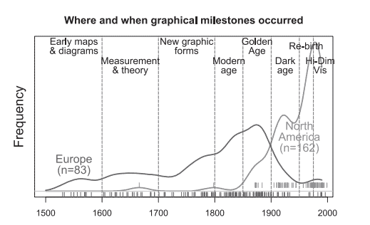
Something even more remarkable occurred in the latter part of the nineteenth century, as many forces combined to produce the perfect storm for data graphics, in what we call the Golden Age of Graphics (Chapter 7). By the mid-1800s, vast quantities of data on important social issues (commerce, disease, literacy, crime) had become available in Europe and the United States, so much that one historian called this an “avalanche of numbers.” 16 In the second half of this century some statistical theory was developed to allow their essence to be summarized and sensible comparisons to be made. Technological advances in printing and reproduction now allowed for the broad dissemination of graphic works in color and with a graphic style that

was unavailable previously. Excitement and enthusiasm for graphics were in the air. ${ }^{17}$ The audience was international, but they shared a common visual language and visual thinking.

Another of the key developers of graphic vision was Charles Joseph Minard $[1781-1870]$, a civil engineer in France, who produced what is now applauded as the greatest data-based graphic of all time-a flow map depicting Napoleon’s disastrous Russian campaign of 1812 (see Figure 10.3). Minard used the graphic method to design beautiful thematic maps and diagrams showing all manner of topics of interest to the modern French state during the dawn of national concern for trade, commerce, and transportation: Where to build railroads? How did the US Civil War affect the British mills’ importation of cotton? In these and other graphs, he told graphic stories of immediate visual impact-the message hit the viewer between the eyes. Minard too was driven by an inner vision.

By the end of the nineteenth century, scientists from the United States (Francis Walker in the Census Bureau), France (Émile Cheysson in the Mini stry of Public Works), and others in Germany (Herman Schwabe, August F. W. Crome), Sweden, and elsewhere, began to produce and widely disseminate elaborate and detailed statistical albums tracing and celebrating their nations’ achievements and aspirations. These contain some of the most exquisite graphs ever produced, even to this day. They were resplendent in color and style and revealed a vision of inventive graphic design that serves as a model to emulate and has become part of the language of graphics today. They inspire awe, just as do the cave paintings in Lascaux.

In this chapter we have taken a long-range view of visualizations spanning more than 17,000 years from the Lascaux cave paintings of long extinct auroch bulls to Minard’s equally exquisite depictions of the horrors of the Napoleonic Wars. In both these cases, and in many in between, visualizations have painlessly provided memorable understanding for those who look at them. Over the course of centuries, rising visual thinking was expressed in diagrams, maps, and graphs. A universal language of visualizations was used to communicate both quantitative and qualitative information, to uncover complex phenomena, to support, or refute, scientific claims. In the balance of this book we will elaborate and illustrate the wonders of visual communication and welcome you along on the journey.

数据可视化代考

统计代写|数据可视化代写Data visualization代考|The Rise of the Graphic Method and Visual Thinking

Playfair 的图形发明——折线图、条形图和饼图——是当今最常用的图形形式。条形图有点反常：缺乏绘制显示与苏格兰贸易时间线所需的时间序列数据，他使用条形来象征他确实拥有的数据的横截面特征。Playfair 以这种形式承认了 Priestley (1765, 1769) 的优先权，使用细横条在时间线上象征历史人物的寿命（图 1.6）。引起 Playfair 兴趣的是，可以将一段长时间的历史可视化并显示分类（政治家与有学问的人）——所有这些都在一个单一的视图中。

Playfair 的角色至关重要，原因有几个。这不是因为他开发了数据的图形记录；其他人在这方面先于他。事实上，他在 1805 年指出，他的兄弟约翰小时候曾让他保存温度读数的图形记录。但普莱费尔处于一个了不起的位置。由于他与兄弟的密切关系以及与瓦特的关系，他处于科学的边缘。他足够接近了解图解法的价值，但又足够独立于自己的利益，以将它们应用到一个非常不同的领域——经济和金融领域。与现在一样，这些领域往往比科学问题更能吸引更多的观众，而 Playfair 擅长自我推销。15

苏格兰历史学家吉尔伯特·斯图亚特博士在对他的 1786 年《政治先驱报》上的地图集进行评论时写道，
在这部作品中叙述叙述的新方法引起了广泛的关注。所有对国家有任何利益的人，熟悉大致的轮廓，以及与我们的商业有关的重大事实，他们的正当性和权宜之计是毋庸置疑的。这是迄今为止被认为是影响这个对象的最方便、最准确的方式…… 作者在他的每张图表中都添加了观察结果（这些观察结果）……总的来说是公正而精明的；有时深刻…… 非常热烈的掌声肯定是由于他的发明。作为一种新的、独特的、简单的向政治家和商人传达信息的方式。

统计代写|数据可视化代写Data visualization代考|A Golden Age

在 19 世纪下半叶发生了更引人注目的事情，因为许多力量共同产生了数据图形的完美风暴，我们称之为图形的黄金时代（第 7 章）。到 1800 年代中期，关于重要社会问题（商业、疾病、识字、犯罪）的大量数据已在欧洲和美国获得，以至于一位历史学家称其为“数字雪崩”。16 在本世纪下半叶，一些统计理论得到发展，以便总结其本质并进行合理的比较。印刷和复制技术的进步现在允许广泛传播彩色和图形风格的图形作品

以前无法使用。空气中弥漫着对图形的兴奋和热情。17观众是国际化的，但他们有着共同的视觉语言和视觉思维。

图形视觉的另一位主要开发者是查尔斯·约瑟夫·米纳德（Charles Joseph Minard）[1781−1870]，一位法国的土木工程师，他制作了现在被称赞为有史以来最伟大的基于数据的图形——一幅描绘拿破仑在 1812 年灾难性的俄国战役的流程图（见图 10.3）。Minard 使用图形方法设计了精美的专题地图和图表，展示了在国家关注贸易、商业和运输的黎明时期现代法国政府感兴趣的各种主题：在哪里建造铁路？美国内战如何影响英国纺织厂的棉花进口？在这些图表和其他图表中，他讲述了即时视觉冲击的图形故事——信息击中了观众的双眼。米纳德也受到内在愿景的驱使。

到 19 世纪末，来自美国（人口普查局的弗朗西斯·沃克）、法国（Mini stry of Public Works 中的 Émile Cheysson）和德国（Herman Schwabe，August FW Crome）、瑞典的其他科学家，和其他地方，开始制作和广泛传播详尽和详细的统计专辑，追踪和庆祝他们国家的成就和愿望。这些包含一些迄今为止制作的最精美的图表。它们在色彩和风格上都非常出色，并揭​​示了创造性图形设计的愿景，可以作为模仿的模型，并已成为当今图形语言的一部分。它们令人敬畏，就像拉斯科的洞穴壁画一样。

在本章中，我们对跨越 17,000 多年的可视化进行了长期的观察，从拉斯科洞穴壁画中长期灭绝的野牛公牛到米纳德对拿破仑战争恐怖的同样精美的描绘。在这两种情况下，以及介于两者之间的许多情况下，可视化都为那些看到它们的人提供了令人难忘的理解。几个世纪以来，不断上升的视觉思维以图表、地图和图表的形式表达出来。一种通用的可视化语言被用来传达定量和定性信息，揭示复杂现象，支持或反驳科学主张。在本书的其余部分，我们将详细阐述和说明视觉传达的奇迹，并欢迎您一路同行。

统计代写请认准statistics-lab™. statistics-lab™为您的留学生涯保驾护航。

金融工程代写

金融工程是使用数学技术来解决金融问题。金融工程使用计算机科学、统计学、经济学和应用数学领域的工具和知识来解决当前的金融问题，以及设计新的和创新的金融产品。

非参数统计代写

非参数统计指的是一种统计方法，其中不假设数据来自于由少数参数决定的规定模型；这种模型的例子包括正态分布模型和线性回归模型。

广义线性模型代考

广义线性模型（GLM）归属统计学领域，是一种应用灵活的线性回归模型。该模型允许因变量的偏差分布有除了正态分布之外的其它分布。

术语 广义线性模型（GLM）通常是指给定连续和/或分类预测因素的连续响应变量的常规线性回归模型。它包括多元线性回归，以及方差分析和方差分析（仅含固定效应）。

有限元方法代写

有限元方法（FEM）是一种流行的方法，用于数值解决工程和数学建模中出现的微分方程。典型的问题领域包括结构分析、传热、流体流动、质量运输和电磁势等传统领域。

有限元是一种通用的数值方法，用于解决两个或三个空间变量的偏微分方程（即一些边界值问题）。为了解决一个问题，有限元将一个大系统细分为更小、更简单的部分，称为有限元。这是通过在空间维度上的特定空间离散化来实现的，它是通过构建对象的网格来实现的：用于求解的数值域，它有有限数量的点。边界值问题的有限元方法表述最终导致一个代数方程组。该方法在域上对未知函数进行逼近。[1] 然后将模拟这些有限元的简单方程组合成一个更大的方程系统，以模拟整个问题。然后，有限元通过变化微积分使相关的误差函数最小化来逼近一个解决方案。

tatistics-lab作为专业的留学生服务机构，多年来已为美国、英国、加拿大、澳洲等留学热门地的学生提供专业的学术服务，包括但不限于Essay代写，Assignment代写，Dissertation代写，Report代写，小组作业代写，Proposal代写，Paper代写，Presentation代写，计算机作业代写，论文修改和润色，网课代做，exam代考等等。写作范围涵盖高中，本科，研究生等海外留学全阶段，辐射金融，经济学，会计学，审计学，管理学等全球99%专业科目。写作团队既有专业英语母语作者，也有海外名校硕博留学生，每位写作老师都拥有过硬的语言能力，专业的学科背景和学术写作经验。我们承诺100%原创，100%专业，100%准时，100%满意。

随机分析代写

随机微积分是数学的一个分支，对随机过程进行操作。它允许为随机过程的积分定义一个关于随机过程的一致的积分理论。这个领域是由日本数学家伊藤清在第二次世界大战期间创建并开始的。

时间序列分析代写

随机过程，是依赖于参数的一组随机变量的全体，参数通常是时间。 随机变量是随机现象的数量表现，其时间序列是一组按照时间发生先后顺序进行排列的数据点序列。通常一组时间序列的时间间隔为一恒定值（如1秒，5分钟，12小时，7天，1年），因此时间序列可以作为离散时间数据进行分析处理。研究时间序列数据的意义在于现实中，往往需要研究某个事物其随时间发展变化的规律。这就需要通过研究该事物过去发展的历史记录，以得到其自身发展的规律。

回归分析代写

多元回归分析渐进（Multiple Regression Analysis Asymptotics）属于计量经济学领域，主要是一种数学上的统计分析方法，可以分析复杂情况下各影响因素的数学关系，在自然科学、社会和经济学等多个领域内应用广泛。

MATLAB代写

MATLAB 是一种用于技术计算的高性能语言。它将计算、可视化和编程集成在一个易于使用的环境中，其中问题和解决方案以熟悉的数学符号表示。典型用途包括：数学和计算算法开发建模、仿真和原型制作数据分析、探索和可视化科学和工程图形应用程序开发，包括图形用户界面构建MATLAB 是一个交互式系统，其基本数据元素是一个不需要维度的数组。这使您可以解决许多技术计算问题，尤其是那些具有矩阵和向量公式的问题，而只需用 C 或 Fortran 等标量非交互式语言编写程序所需的时间的一小部分。MATLAB 名称代表矩阵实验室。MATLAB 最初的编写目的是提供对由 LINPACK 和 EISPACK 项目开发的矩阵软件的轻松访问，这两个项目共同代表了矩阵计算软件的最新技术。MATLAB 经过多年的发展，得到了许多用户的投入。在大学环境中，它是数学、工程和科学入门和高级课程的标准教学工具。在工业领域，MATLAB 是高效研究、开发和分析的首选工具。MATLAB 具有一系列称为工具箱的特定于应用程序的解决方案。对于大多数 MATLAB 用户来说非常重要，工具箱允许您学习和应用专业技术。工具箱是 MATLAB 函数（M 文件）的综合集合，可扩展 MATLAB 环境以解决特定类别的问题。可用工具箱的领域包括信号处理、控制系统、神经网络、模糊逻辑、小波、仿真等。

R语言代写	问卷设计与分析代写
PYTHON代写	回归分析与线性模型代写
MATLAB代写	方差分析与试验设计代写
STATA代写	机器学习/统计学习代写
SPSS代写	计量经济学代写
EVIEWS代写	时间序列分析代写
EXCEL代写	深度学习代写
SQL代写	各种数据建模与可视化代写

如果你也在 怎样代写数据可视化Data visualization这个学科遇到相关的难题，请随时右上角联系我们的24/7代写客服。

数据可视化是将信息转化为视觉背景的做法，如地图或图表，使数据更容易被人脑理解并从中获得洞察力。数据可视化的主要目标是使其更容易在大型数据集中识别模式、趋势和异常值。

statistics-lab™ 为您的留学生涯保驾护航 在代写数据可视化Data visualization方面已经树立了自己的口碑, 保证靠谱, 高质且原创的统计Statistics代写服务。我们的专家在代写数据可视化Data visualization代写方面经验极为丰富，各种代写数据可视化Data visualization相关的作业也就用不着说。

我们提供的数据可视化Data visualization及其相关学科的代写，服务范围广, 其中包括但不限于:

• Statistical Inference 统计推断
• Statistical Computing 统计计算
• Advanced Probability Theory 高等概率论
• Advanced Mathematical Statistics 高等数理统计学
• (Generalized) Linear Models 广义线性模型
• Statistical Machine Learning 统计机器学习
• Longitudinal Data Analysis 纵向数据分析
• Foundations of Data Science 数据科学基础

统计代写|数据可视化代写Data visualization代考|Connecting Data with Pictures

As we’ve seen, initial visualizations were of something concrete and specific in the world: a majestic auroch bull in motion, diagrams of wrestling moves, and maps of just a city or of the entire known world. But another branch of visualization was developing too, which depicted an abstract and theoretical world. A century before Descartes formalized his eponymous coordinates, Nicole Oresme in Padua illustrated some of the possible laws of motion in the book Tractus de latitudunus forarum, the “latitude of forms” (see Figure 2.2). Galileo and Newton would later make the study of motion precise, but Oresme had the idea to consider some alternatives and show them in a graph.

What was still lacking was a connection between empirical observationsnumbers-and pictures to convey them to the eye. Natural philosophy-how we learn about the world-had long had two distinct views, rationalism and empiricism, which date back at least to Plato and Aristotle. The philosophical debate has many branches, but the essential contrast was of the role of sensory experience: using observations and data in deriving knowledge, making decisions, and formulating natural laws.

Rationalists claimed that there were some innate or intuitive ideas (a point or line, the idea of language); larger ideas (a triangle or square, words for things versus words for actions) could be deduced by human intellect. For Descartes, one of the founders of seventeenth-century rationalism, the argument was captured in his famous proclamation, “I think, therefore I am.” Analytic geometry was the result of mathematical reasoning applied to geometry, but Descartes also applied this approach to the mind-body problem (determining what distinguishes the corporal self, composed of matter, from the ethereal mind and soul). The laws of the universe are fixed, and they can be discovered by reason. Observations and data were useful, but they only play a supporting role.

Empiricists claimed that knowledge and natural law had to be based fundamentally on empirical evidence, not authority or abstract reasoning. The idea of a scientific method based on observation stems from Roger Bacon [1214-1292], who observed that “reasoning draws a conclusion, but does not make the conclusion certain, unless the mind discovers it by the path of experience” (Bacon, Opus Majus c. 1267; translation from Robert Burke (2002) The Opus Majus of Roger Bacon Part 2. p. 583 ).

统计代写|数据可视化代写Data visualization代考|Seeing the Unexpected

Graphs that were in existence before 1800 , the time of William Playfair (see Chapter 5), largely grew out of the same rationalist tradition that yielded Descartes’s coordinate geometry-the plotting of curves on the basis of an a priori mathematical expression (e.g., Oresme’s “pipes,” shown in Figure 2.2).
The plotting of real data had a remarkable, and largely unanticipated, benefit. It often forced viewers to see what they hadn’t expected. The frequency with which this happened gave birth to the empirical modern approach to science which welcomes the plotting of observed data values with the goal of investigating suggestive patterns.

This was particularly true of Playfair’s graphs, most of which showed mundane economic data over time: balance of trade with other countries, the national debt, and so forth. But these had never been seen before in a way that could suggest patterns, trends, and explanations. In this period, the idea of a graph of numbers, supporting an argument based on evidence, was born.
This crucial change in view of the value of graphs in relation to evidence and explanations has a more nuanced history than we can tell here. However, the revolution seems to have begun in 1665 with the invention of the barometer and graphic recording devices, which used pens driven on paper by a measuring instrument. ${ }^{9}$ Readings from this instrument inspired the eponymous Robert Plot to record the barometric pressure in Oxford every day of 1684 and summarize his findings in a strikingly contemporary graph that he called a “History of the Weather” (Figure 1.4).

This graph is not a beautiful example of a data plot. It looks more like a recording of an old polygraph or cardiac ECG monitor-a bunch of squiggly lines on a dark gray background, with ruled lines that further obscure the data. But the visual insight he had from this, and what he could see as an eventual wider use of plots of the weather, was important. His idea of recording a history of weather made the phenomenon of barometric pressure subject to visual inspection and scientific thought.

数据可视化代考

统计代写|数据可视化代写Data visualization代考|Connecting Data with Pictures

正如我们所看到的，最初的可视化是世界上具体而具体的东西：一头雄伟的野牛运动，摔跤动作的图表，以及只是一个城市或整个已知世界的地图。但可视化的另一个分支也在发展，它描绘了一个抽象的理论世界。在笛卡尔正式确定其同名坐标的一个世纪之前，帕多瓦的 Nicole Oresme 在 Tractus de latitudunus forarum （“形式的纬度”）一书中说明了一些可能的运动定律（见图 2.2）。伽利略和牛顿后来使运动研究变得精确，但奥雷斯梅想到了考虑一些替代方案并将它们显示在图表中。

仍然缺乏的是经验观察数字和图片之间的联系，以将它们传达给眼睛。自然哲学——我们如何了解世界——长期以来有两种截然不同的观点，理性主义和经验主义，至少可以追溯到柏拉图和亚里士多德。哲学辩论有许多分支，但本质上的对比是感官体验的作用：使用观察和数据来获取知识、做出决定和制定自然法则。

理性主义者声称存在一些与生俱来的或直觉的观念（点或线，语言的观念）；更大的想法（三角形或正方形，事物的词与行动的词）可以通过人类的智力推断出来。对于 17 世纪理性主义的创始人之一笛卡尔来说，这一论点体现在他著名的宣言“我思故我在”中。解析几何是应用于几何的数学推理的结果，但笛卡尔也将这种方法应用于身心问题（确定由物质组成的肉体自我与空灵的心灵和灵魂的区别）。宇宙的规律是固定的，可以通过理性来发现。观察和数据是有用的，但它们只起辅助作用。

经验主义者声称，知识和自然法必须从根本上基于经验证据，而不是权威或抽象推理。基于观察的科学方法的想法源于罗杰·培根 [1214-1292]，他观察到“推理得出结论，但不能确定结论，除非头脑通过经验的途径发现它”（培根， Opus Majus c. 1267；翻译自 Robert Burke (2002) The Opus Majus of Roger Bacon Part 2. p. 583 )。

统计代写|数据可视化代写Data visualization代考|Seeing the Unexpected

1800 年之前存在的图，即威廉·普莱费尔（William Playfair）时代（见第 5 章），很大程度上源于产生笛卡尔坐标几何的理性主义传统——基于先验数学表达式（例如，Oresme 的“管道”，如图 2.2 所示）。
真实数据的绘图具有显着的，而且在很大程度上是出乎意料的好处。它经常迫使观众看到他们没有预料到的东西。这种情况发生的频率催生了现代经验的科学方法，该方法欢迎绘制观察到的数据值，目的是调查暗示模式。

Playfair 的图表尤其如此，其中大部分显示了随时间推移的普通经济数据：与其他国家的贸易平衡、国家债务等等。但这些以前从未以可以暗示模式、趋势和解释的方式出现。在这一时期，数字图表的想法诞生了，它支持基于证据的论点。
鉴于图表与证据和解释相关的价值，这一关键变化的历史比我们在这里所能讲述的更为微妙。然而，随着气压计和图形记录设备的发明，这场革命似乎始于 1665 年，这些设备使用由测量仪器在纸上驱动的笔。9该仪器的读数启发了同名的罗伯特·普洛特（Robert Plot）记录 1684 年每天牛津的气压，并将他的发现总结在一张引人注目的当代图表中，他称之为“天气史”（图 1.4）。

该图不是数据图的漂亮示例。它看起来更像是旧测谎仪或心脏心电图监视器的记录——深灰色背景上的一堆波浪线，带有进一步模糊数据的格线。但他从中获得的视觉洞察力，以及他所看到的最终更广泛地使用天气图，是很重要的。他记录天气历史的想法使大气压力现象受到视觉检查和科学思考。

统计代写请认准statistics-lab™. statistics-lab™为您的留学生涯保驾护航。

金融工程代写

金融工程是使用数学技术来解决金融问题。金融工程使用计算机科学、统计学、经济学和应用数学领域的工具和知识来解决当前的金融问题，以及设计新的和创新的金融产品。

非参数统计代写

非参数统计指的是一种统计方法，其中不假设数据来自于由少数参数决定的规定模型；这种模型的例子包括正态分布模型和线性回归模型。

广义线性模型代考

广义线性模型（GLM）归属统计学领域，是一种应用灵活的线性回归模型。该模型允许因变量的偏差分布有除了正态分布之外的其它分布。

术语 广义线性模型（GLM）通常是指给定连续和/或分类预测因素的连续响应变量的常规线性回归模型。它包括多元线性回归，以及方差分析和方差分析（仅含固定效应）。

有限元方法代写

有限元方法（FEM）是一种流行的方法，用于数值解决工程和数学建模中出现的微分方程。典型的问题领域包括结构分析、传热、流体流动、质量运输和电磁势等传统领域。

有限元是一种通用的数值方法，用于解决两个或三个空间变量的偏微分方程（即一些边界值问题）。为了解决一个问题，有限元将一个大系统细分为更小、更简单的部分，称为有限元。这是通过在空间维度上的特定空间离散化来实现的，它是通过构建对象的网格来实现的：用于求解的数值域，它有有限数量的点。边界值问题的有限元方法表述最终导致一个代数方程组。该方法在域上对未知函数进行逼近。[1] 然后将模拟这些有限元的简单方程组合成一个更大的方程系统，以模拟整个问题。然后，有限元通过变化微积分使相关的误差函数最小化来逼近一个解决方案。

tatistics-lab作为专业的留学生服务机构，多年来已为美国、英国、加拿大、澳洲等留学热门地的学生提供专业的学术服务，包括但不限于Essay代写，Assignment代写，Dissertation代写，Report代写，小组作业代写，Proposal代写，Paper代写，Presentation代写，计算机作业代写，论文修改和润色，网课代做，exam代考等等。写作范围涵盖高中，本科，研究生等海外留学全阶段，辐射金融，经济学，会计学，审计学，管理学等全球99%专业科目。写作团队既有专业英语母语作者，也有海外名校硕博留学生，每位写作老师都拥有过硬的语言能力，专业的学科背景和学术写作经验。我们承诺100%原创，100%专业，100%准时，100%满意。

随机分析代写

随机微积分是数学的一个分支，对随机过程进行操作。它允许为随机过程的积分定义一个关于随机过程的一致的积分理论。这个领域是由日本数学家伊藤清在第二次世界大战期间创建并开始的。

时间序列分析代写

随机过程，是依赖于参数的一组随机变量的全体，参数通常是时间。 随机变量是随机现象的数量表现，其时间序列是一组按照时间发生先后顺序进行排列的数据点序列。通常一组时间序列的时间间隔为一恒定值（如1秒，5分钟，12小时，7天，1年），因此时间序列可以作为离散时间数据进行分析处理。研究时间序列数据的意义在于现实中，往往需要研究某个事物其随时间发展变化的规律。这就需要通过研究该事物过去发展的历史记录，以得到其自身发展的规律。

回归分析代写

多元回归分析渐进（Multiple Regression Analysis Asymptotics）属于计量经济学领域，主要是一种数学上的统计分析方法，可以分析复杂情况下各影响因素的数学关系，在自然科学、社会和经济学等多个领域内应用广泛。

MATLAB代写

MATLAB 是一种用于技术计算的高性能语言。它将计算、可视化和编程集成在一个易于使用的环境中，其中问题和解决方案以熟悉的数学符号表示。典型用途包括：数学和计算算法开发建模、仿真和原型制作数据分析、探索和可视化科学和工程图形应用程序开发，包括图形用户界面构建MATLAB 是一个交互式系统，其基本数据元素是一个不需要维度的数组。这使您可以解决许多技术计算问题，尤其是那些具有矩阵和向量公式的问题，而只需用 C 或 Fortran 等标量非交互式语言编写程序所需的时间的一小部分。MATLAB 名称代表矩阵实验室。MATLAB 最初的编写目的是提供对由 LINPACK 和 EISPACK 项目开发的矩阵软件的轻松访问，这两个项目共同代表了矩阵计算软件的最新技术。MATLAB 经过多年的发展，得到了许多用户的投入。在大学环境中，它是数学、工程和科学入门和高级课程的标准教学工具。在工业领域，MATLAB 是高效研究、开发和分析的首选工具。MATLAB 具有一系列称为工具箱的特定于应用程序的解决方案。对于大多数 MATLAB 用户来说非常重要，工具箱允许您学习和应用专业技术。工具箱是 MATLAB 函数（M 文件）的综合集合，可扩展 MATLAB 环境以解决特定类别的问题。可用工具箱的领域包括信号处理、控制系统、神经网络、模糊逻辑、小波、仿真等。

R语言代写	问卷设计与分析代写
PYTHON代写	回归分析与线性模型代写
MATLAB代写	方差分析与试验设计代写
STATA代写	机器学习/统计学习代写
SPSS代写	计量经济学代写
EVIEWS代写	时间序列分析代写
EXCEL代写	深度学习代写
SQL代写	各种数据建模与可视化代写

如果你也在 怎样代写数据可视化Data visualization这个学科遇到相关的难题，请随时右上角联系我们的24/7代写客服。

数据可视化是将信息转化为视觉背景的做法，如地图或图表，使数据更容易被人脑理解并从中获得洞察力。数据可视化的主要目标是使其更容易在大型数据集中识别模式、趋势和异常值。

statistics-lab™ 为您的留学生涯保驾护航 在代写数据可视化Data visualization方面已经树立了自己的口碑, 保证靠谱, 高质且原创的统计Statistics代写服务。我们的专家在代写数据可视化Data visualization代写方面经验极为丰富，各种代写数据可视化Data visualization相关的作业也就用不着说。

我们提供的数据可视化Data visualization及其相关学科的代写，服务范围广, 其中包括但不限于:

• Statistical Inference 统计推断
• Statistical Computing 统计计算
• Advanced Probability Theory 高等概率论
• Advanced Mathematical Statistics 高等数理统计学
• (Generalized) Linear Models 广义线性模型
• Statistical Machine Learning 统计机器学习
• Longitudinal Data Analysis 纵向数据分析
• Foundations of Data Science 数据科学基础

统计代写|数据可视化代写Data visualization代考|In the Beginning

It was only much later that words for objects and concepts found a physical expression in inscriptions, initially as pictographs on clay tablets in Mesopotamia around 3100 BCE and independently in Egypt, China, and elsewhere. These were picture-writing systems: a sequence of pictographs, ${ }^{1}$ such as Egyptian hieroglyphs, could be used to tell a story of a conquest or the life of a pharaoh or even record the mundane facts of a harvest or a debt.

Written language originated in pictures. Like later alphabetic writing systems, the key feature was that they were productive: A limited number of iconic symbols could be used to express a nearly infinite number of thoughts and ideas. However, the first physical inscriptions did not appear as a sign by the watering hole warning of a lion or in a marriage proposal; rather, they were used to record numbers.

The idea of a number is very old indeed, and ancient ways of writing down numbers can be traced back to Paleolithic tally sticks (dating from the Aurignacian, approximately 30,000 years ago), in which notches were cut into a bone, ostensibly to represent counts of something of interest, such as to keep track of domestic animals. A notch was made when an animal was released to pasture; later, when it returned, the shepherd’s thumb would be moved down the stick, notch by notch. If the last returning animal ended with the last notch, the shepherd would be assured that all was well. Such a system, while a vast improvement on trusting counts to memory, had room for improvement. Adding an additional animal (a birth) was easy-just add another notch-but subtracting (due to a predator in the neighborhood or mutton for lunch) was more difficult and might require carving a new stick. Keeping separate track of different kinds of animals (say, goats and sheep) could be done with additional sticks for each type, but it would quickly become cumbersome to carry them around and to remember which was which.

Over time, the system of counting sticks evolved, as shown in Figure 1.1. Around 3300 BCE the Sumerians in Mesopotamia used cuneiform symbols on clay tablets to record information about trade and agriculture (Figure 1.1a). The pre-Columbian Incans in South America transformed counting sticks into quipus, which were ropes into which were tied knots that served the same role as notches. But knots could be untied, allowing subtraction (Figure 1.1b). Also, two or more such ropes, each representing a different kind of animal, could be tied together and easily carried wrapped around the waist or thrown over the shoulder.

统计代写|数据可视化代写Data visualization代考|1 Some of the graphic forms used to represent numbers

(a) A clay cuneiform tablet dated as 3300-3100 BCE, giving an account of yields of barley; (b) quipus, a system of knots tied in ropes used by South American Incas, around $1000 \mathrm{CE}$; (c) symbols used in Mayan culture, around $500 \mathrm{CE}$, showing the numbers $0-19 ;$ (d) a scheme proposed by John W. Tukey (1977) to tally counts of observations by hand, using dots and lines in groups of 10. Sources: (a) Britannica.com; (b) L. Leland Locke, The Ancient Quipu, Washington, DC: The American Museum of Natural History, 1923, fig. $1_{\text {; }}$ (c) Neuromancer2K4 / Bryan Derksen / Wikimedia Commons / GNU Free Documentation License; (d) Pinethicket / Wikimedia Commons/GNU Free Documentation License.

The Mayan culture around 100 BCE used a sophisticated number system, probably the most advanced in the world at the time (Figure 1.1c). It used base 20 , most likely developed from counting on fingers and toes. The numerals from 0 to 19 used only three symbols, representing zero (a shell shape), one (a dot), and five (a horizontal bar). After the number 19, larger numbers were written in a vertical place value format using powers of $20: 1,20,400,8000$, and so on; thus, the number 826 was represented by symbols for $(2 \times 400)+$ $(1 \times 20)+6$. This made it relatively easy to both add and subtract.

统计代写|数据可视化代写Data visualization代考|The Evolution of Pictures

Perhaps the best known of the very early examples of human visualizations are found in the Lascaux caves near the French village of Montignac in the Dorgogne region. The cave walls contain nearly 2,000 remarkable drawings of animals, human-like figures, and abstract or geometric signs, which carbon dating has estimated to be about 17,300 years old. The inhabitants of these caves were among the oldest known modern humans (Homo sapiens), called Cro-Magnon man.

A small section of what is now called the Chamber of the Bulls is shown in Plate 1. It is hard to get a sense of their majesty from this one image, but the collection is spectacular by any measure. Henri Édouard Prosper Breuil ${ }^{4}$ [1877-1961], the first archaeological expert to view the cave, called the drawings in the Axial Gallery of the cave “The Sistine Chapel of prehistoric man.” After seeing them in the public re-creation of Lascaux II, a modern viewer would find it difficult to ever again think of these ancestors as primitive people.

It may seem surprising for us to start this tour of the history of visualization so early, and with images, that, although impressive artistically, might be considered too far afield. Yet, there are deeper lessons here. When we view images from this history, our questions usually are: What were they thinking? Why did they draw them? What can we learn from them today? Indeed, such questions form a main theme of this book.

We can only speculate on these early cave paintings. A naive view suggests that they might reflect a celebratory display of past hunting success. But this is wrong-other evidence shows that these early dwellers in the Vézère valley hunted reindeer primarily, and there are no images of reindeer on the cave walls.

数据可视化代考

统计代写|数据可视化代写Data visualization代考|In the Beginning

直到很久以后，物体和概念的文字才在铭文中找到了物理表达，最初是公元前 3100 年左右在美索不达米亚的泥板上的象形文字，后来在埃及、中国和其他地方独立出现。这些是图画书写系统：一系列象形文字，1例如埃及的象形文字，可以用来讲述征服的故事或法老的生平，甚至可以记录收成或债务的平凡事实。

书面语言起源于图片。与后来的字母书写系统一样，关键特征是它们的生产力：有限数量的标志性符号可用于表达几乎无限数量的思想和想法。然而，最初的物理铭文并没有作为狮子的水坑警告或求婚的标志出现。相反，它们被用来记录数字。

数字的概念确实非常古老，写下数字的古老方式可以追溯到旧石器时代的计数棒（可追溯到大约 30,000 年前的 Aurignacian），其中的凹口被切入骨头，表面上代表计数感兴趣的事情，例如跟踪家畜。当动物被释放到牧场时，会形成一个缺口；后来，当它回来时，牧羊人的拇指会顺着棍子一点一点地移动。如果最后一只返回的动物以最后一个缺口结束，牧羊人将确信一切都很好。这样的系统虽然在信任计数方面有了很大的改进，但仍有改进的余地。添加额外的动物（出生）很容易——只需添加另一个缺口——但减去（由于附近有捕食者或午餐吃羊肉）更困难，可能需要雕刻一根新棍子。单独跟踪不同种类的动物（例如山羊和绵羊）可以通过为每种类型添加额外的棍子来完成，但是携带它们并记住哪个是哪个很快就会变得很麻烦。

随着时间的推移，计数棒系统不断发展，如图 1.1 所示。大约公元前 3300 年，美索不达米亚的苏美尔人在泥板上使用楔形文字符号来记录有关贸易和农业的信息（图 1.1a）。南美洲前哥伦布时期的印加人将计数棒变成了quipus，它是绳索，上面系着结，起到与凹口相同的作用。但是可以解开结，允许减法（图 1.1b）。此外，两根或多根这样的绳子，每根都代表一种不同的动物，可以绑在一起，很容易绕在腰间或挂在肩膀上。

统计代写|数据可视化代写Data visualization代考|1 Some of the graphic forms used to represent numbers

(a) 公元前 3300-3100 年的粘土楔形文字板，记载了大麦的产量；(b) quipus，一种系在南美印加人使用的绳索上的结系统，在1000C和; (c) 玛雅文化中使用的符号，周围500C和, 显示数字0−19;(d) John W. Tukey (1977) 提出的一种方案，使用 10 个一组的点和线来手动统计观察次数。资料来源：(a) Britannica.com；(b) L. Leland Locke，The Ancient Quipu，华盛顿特区：美国自然历史博物馆，1923 年，图。1; (c) Neuromancer2K4 / Bryan Derksen / Wikimedia Commons / GNU 自由文档许可证；(d) Pinethicket/Wikimedia Commons/GNU 自由文档许可证。

公元前 100 年左右的玛雅文化使用了一种复杂的数字系统，这可能是当时世界上最先进的（图 1.1c）。它使用 20 为底数，很可能是从数手指和脚趾发展而来的。从 0 到 19 的数字只使用了三个符号，分别代表零（贝壳形状）、一（点）和五（横条）。在数字 19 之后，更大的数字以垂直位值格式使用20:1,20,400,8000， 等等; 因此，数字 826 用符号表示(2×400)+ (1×20)+6. 这使得加法和减法都相对容易。

统计代写|数据可视化代写Data visualization代考|The Evolution of Pictures

在多尔戈涅地区的法国蒙蒂尼亚克村附近的拉斯科洞穴中，可能最著名的人类可视化的早期例子。洞穴墙壁包含近 2,000 幅非凡的动物图画、类人人物以及抽象或几何符号，碳测年法估计这些图画已有 17,300 年的历史。这些洞穴的居民是已知最古老的现代人类（智人）之一，被称为克罗马农人。

图 1 展示了现在被称为公牛厅的一小部分。很难从这张图片中感受到它们的威严，但无论以何种标准衡量，这个收藏都非常壮观。Henri Édouard Prosper Breuil4[1877-1961]，第一位观察该洞穴的考古专家，将洞穴轴向画廊中的图纸称为“史前人类的西斯廷教堂”。在公开再现拉斯科二世之后，现代观众会发现很难再将这些祖先视为原始人。

对于我们来说，如此早地开始这次可视化历史之旅似乎令人惊讶，而且图像虽然在艺术上令人印象深刻，但可能被认为太遥远了。然而，这里有更深层次的教训。当我们查看这段历史的图像时，我们的问题通常是：他们在想什么？他们为什么画它们？今天我们可以从他们身上学到什么？事实上，这些问题构成了本书的一个主题。

我们只能推测这些早期的洞穴壁画。一种天真的观点表明，它们可能反映了过去狩猎成功的庆祝展示。但这是错误的——其他证据表明，Vézère 山谷的这些早期居民主要猎杀驯鹿，而洞穴墙壁上没有驯鹿的图像。

统计代写请认准statistics-lab™. statistics-lab™为您的留学生涯保驾护航。

金融工程代写

金融工程是使用数学技术来解决金融问题。金融工程使用计算机科学、统计学、经济学和应用数学领域的工具和知识来解决当前的金融问题，以及设计新的和创新的金融产品。

非参数统计代写

非参数统计指的是一种统计方法，其中不假设数据来自于由少数参数决定的规定模型；这种模型的例子包括正态分布模型和线性回归模型。

广义线性模型代考

广义线性模型（GLM）归属统计学领域，是一种应用灵活的线性回归模型。该模型允许因变量的偏差分布有除了正态分布之外的其它分布。

术语 广义线性模型（GLM）通常是指给定连续和/或分类预测因素的连续响应变量的常规线性回归模型。它包括多元线性回归，以及方差分析和方差分析（仅含固定效应）。

有限元方法代写

有限元方法（FEM）是一种流行的方法，用于数值解决工程和数学建模中出现的微分方程。典型的问题领域包括结构分析、传热、流体流动、质量运输和电磁势等传统领域。

有限元是一种通用的数值方法，用于解决两个或三个空间变量的偏微分方程（即一些边界值问题）。为了解决一个问题，有限元将一个大系统细分为更小、更简单的部分，称为有限元。这是通过在空间维度上的特定空间离散化来实现的，它是通过构建对象的网格来实现的：用于求解的数值域，它有有限数量的点。边界值问题的有限元方法表述最终导致一个代数方程组。该方法在域上对未知函数进行逼近。[1] 然后将模拟这些有限元的简单方程组合成一个更大的方程系统，以模拟整个问题。然后，有限元通过变化微积分使相关的误差函数最小化来逼近一个解决方案。

tatistics-lab作为专业的留学生服务机构，多年来已为美国、英国、加拿大、澳洲等留学热门地的学生提供专业的学术服务，包括但不限于Essay代写，Assignment代写，Dissertation代写，Report代写，小组作业代写，Proposal代写，Paper代写，Presentation代写，计算机作业代写，论文修改和润色，网课代做，exam代考等等。写作范围涵盖高中，本科，研究生等海外留学全阶段，辐射金融，经济学，会计学，审计学，管理学等全球99%专业科目。写作团队既有专业英语母语作者，也有海外名校硕博留学生，每位写作老师都拥有过硬的语言能力，专业的学科背景和学术写作经验。我们承诺100%原创，100%专业，100%准时，100%满意。

随机分析代写

随机微积分是数学的一个分支，对随机过程进行操作。它允许为随机过程的积分定义一个关于随机过程的一致的积分理论。这个领域是由日本数学家伊藤清在第二次世界大战期间创建并开始的。

时间序列分析代写

随机过程，是依赖于参数的一组随机变量的全体，参数通常是时间。 随机变量是随机现象的数量表现，其时间序列是一组按照时间发生先后顺序进行排列的数据点序列。通常一组时间序列的时间间隔为一恒定值（如1秒，5分钟，12小时，7天，1年），因此时间序列可以作为离散时间数据进行分析处理。研究时间序列数据的意义在于现实中，往往需要研究某个事物其随时间发展变化的规律。这就需要通过研究该事物过去发展的历史记录，以得到其自身发展的规律。

回归分析代写

多元回归分析渐进（Multiple Regression Analysis Asymptotics）属于计量经济学领域，主要是一种数学上的统计分析方法，可以分析复杂情况下各影响因素的数学关系，在自然科学、社会和经济学等多个领域内应用广泛。

MATLAB代写

MATLAB 是一种用于技术计算的高性能语言。它将计算、可视化和编程集成在一个易于使用的环境中，其中问题和解决方案以熟悉的数学符号表示。典型用途包括：数学和计算算法开发建模、仿真和原型制作数据分析、探索和可视化科学和工程图形应用程序开发，包括图形用户界面构建MATLAB 是一个交互式系统，其基本数据元素是一个不需要维度的数组。这使您可以解决许多技术计算问题，尤其是那些具有矩阵和向量公式的问题，而只需用 C 或 Fortran 等标量非交互式语言编写程序所需的时间的一小部分。MATLAB 名称代表矩阵实验室。MATLAB 最初的编写目的是提供对由 LINPACK 和 EISPACK 项目开发的矩阵软件的轻松访问，这两个项目共同代表了矩阵计算软件的最新技术。MATLAB 经过多年的发展，得到了许多用户的投入。在大学环境中，它是数学、工程和科学入门和高级课程的标准教学工具。在工业领域，MATLAB 是高效研究、开发和分析的首选工具。MATLAB 具有一系列称为工具箱的特定于应用程序的解决方案。对于大多数 MATLAB 用户来说非常重要，工具箱允许您学习和应用专业技术。工具箱是 MATLAB 函数（M 文件）的综合集合，可扩展 MATLAB 环境以解决特定类别的问题。可用工具箱的领域包括信号处理、控制系统、神经网络、模糊逻辑、小波、仿真等。

R语言代写	问卷设计与分析代写
PYTHON代写	回归分析与线性模型代写
MATLAB代写	方差分析与试验设计代写
STATA代写	机器学习/统计学习代写
SPSS代写	计量经济学代写
EVIEWS代写	时间序列分析代写
EXCEL代写	深度学习代写
SQL代写	各种数据建模与可视化代写

如果你也在 怎样代写数据可视化Data visualization这个学科遇到相关的难题，请随时右上角联系我们的24/7代写客服。

数据可视化是将信息转化为视觉背景的做法，如地图或图表，使数据更容易被人脑理解并从中获得洞察力。数据可视化的主要目标是使其更容易在大型数据集中识别模式、趋势和异常值。

statistics-lab™ 为您的留学生涯保驾护航 在代写数据可视化Data visualization方面已经树立了自己的口碑, 保证靠谱, 高质且原创的统计Statistics代写服务。我们的专家在代写数据可视化Data visualization代写方面经验极为丰富，各种代写数据可视化Data visualization相关的作业也就用不着说。

我们提供的数据可视化Data visualization及其相关学科的代写，服务范围广, 其中包括但不限于:

• Statistical Inference 统计推断
• Statistical Computing 统计计算
• Advanced Probability Theory 高等概率论
• Advanced Mathematical Statistics 高等数理统计学
• (Generalized) Linear Models 广义线性模型
• Statistical Machine Learning 统计机器学习
• Longitudinal Data Analysis 纵向数据分析
• Foundations of Data Science 数据科学基础

统计代写|数据可视化代写Data visualization代考|Figures should be Aesthetically Appropriate

It’s surprisingly common to see figures that are pixelated, whose labels are too small (or too large) relative to the text, or whose font family is inconsistent with the text. Another common issue (especially in presentations) is the choice of colors: if you have a dark background in your figure, the choice of colors must take that into account, otherwise it will be much harder for the audience to read your slides-especially considering that projectors often don’t have great contrast and resolution.

Your figures should look crisp even when you zoom in, and they should not distract the reader from what really matters (again: less is more). You should have clear labels along the axes (when needed) and an informative caption, and your use of color should serve a purpose-remember that using colors can actually be a problem in some journals. In reality, it’s usually possible to remove the colors from a figure and use some other dimension to convey the same information-we will exercise that throughout the book.

Fig. 2.4, like the figure we discussed earlier in this chapter (Fig. 2.3), shows a bar plot. Here, however, we have three dimensions: the $y$-axis shows the change in score (e.g., pre- and post-test) of the hypothetical study mentioned earlier; the $x$-axis shows the different native languages of the participants in said study; and the fill of the bars discriminates the two methods under examination. Note that the font sizes are appropriate (not too small, not too large). In addition, the key is positioned at the top of the figure, not at the side. This allows us to better use the space (i.e., increase the horizontal size of the figure itself). No colors are needed here, since the fill of the bars represents a factor with only two levels (“In-person” and “Online”). Finally, the bars represent the mean improvement, but the plot also shows standard errors from the mean. If the plot only showed means, it would be considerably less informative, as we would know nothing about how certain we are about the means in question (i.e., we would not incorporate information about the variance in the data).

统计代写|数据可视化代写Data visualization代考|Basic Statistics in R

So far in this chapter we have covered a lot. We installed $\mathrm{R}$ and RStudio, discussed RStudio’s interface, and explored some $R$ basics with a number of code blocks, which led us to ggplot2 and figures in the previous section. Once we have a figure, the natural next step is to statistically analyze the patterns shown in said figure. Thus, in this section of the chapter, we will turn to some basic statistical concepts-this will be a good opportunity to review some concepts that will be used throughout the book. We’ll first start with one of the most basic concepts, namely, sampling.

Assume we want to collect data on proficiency scores from 20 learners. To simulate an entire population of learners containing, say, 1 million data points, we can use the function rnorm(), which randomly generates numbers following a normal (Gaussian) distribution ${ }^{25}$ (there’s no reason to assume that proficiency scores are not normally distributed here). Create a variable called pop and assign to it $\operatorname{rnorm}(\mathrm{n}=1000000$, mean $=85, \mathrm{sd}=8)$-you can even do this in the console, without creating a new script, since it will be a simple exercise. This will generate one million scores normally distributed around a mean $(\mu)$ of 85 points with a standard deviation $(\sigma)$ of 8 points. In reality, we never know what the mean and standard deviations are for our population, but here we do since we are the ones simulating the data. You can check that both $\mu$ and $\sigma$ are roughly 85 and 8 , respectively, by running mean(pop) and sd(pop) you won’t get exact numbers, but they should be very close to the parameter values we set using rnorm().

Next, let’s sample 20 values from pop-this is equivalent to collecting data from 20 learners from a population of one million learners. To do that, create a new variable, sam, and assign to it sample $(x=$ pop, size $=20)$. Now, run mean( ) and sd() on sam, and you should get a sample mean $(\bar{x})$ and a sample standard deviation $(s)$ that should be very similar to the true population parameters $(\mu, \sigma)$ we defined earlier. This is a quick and easy way to see sampling at work: we define the population ourselves, so it’s straightforward to check how representative our sample is.

统计代写|数据可视化代写Data visualization代考|What’s Your Research Question

If you already have actual data, that means you have long passed the stages of formulating a research question and working on your study design. Having a relevant research question is as important as it is difficult-see Mackey and Gass (2016, ch. 1). Great studies are in part the result of great research questions. Your question will dictate how you will design your study, which in turn will dictate how you will analyze your data. Understanding all three components is essential. After all, you may have an interesting question but fail to have an adequate study design, or you may have both a relevant question and an appropriate study design but realize that you don’t know how to analyze the data.

The hypothetical dataset in question (long) consists of two groups of participants (control and target) as well as three sets of test scores-we will examine more complex and realistic datasets later on, but for now our tibble long will be sufficient. Suppose that our study examines the effects of a particular pedagogical approach on students’ scores, as briefly mentioned earlier. For illustrative purposes, let’s assume that we want to compare a student-centered approach (e.g., workshop-based), our targets (treatment group), to a teacher-centered approach (e.g., lecture-based), our controls, so we are comparing two clearly defined approaches (two groups). Next, we must be able to measure scores. To do that, we have decided to administer three tests (e.g., a pre-test (testA), a post-test (testB), and a delayed post-test (testC), as alluded to earlier). With that in mind, we can ask specific questions: is the improvement from test $A$ to testB statistically different between controls and targets? How about from testA to testC? These questions must speak directly to your overarching research question. Finally, in addition to a research question, you may have a directional hypothesis, for example, that a lecture-based approach will lead to lower scores overall, or a non-directional hypothesis, for example, that there will be some difference in learning between the two approaches, but which one will be better is unknown. Let’s now go over some basic stats assuming the hypothetical context in question.

数据可视化代考

统计代写|数据可视化代写Data visualization代考|Figures should be Aesthetically Appropriate

看到像素化的图形，其标签相对于文本太小（或太大），或者其字体系列与文本不一致的情况令人惊讶地常见。另一个常见的问题（尤其是在演示文稿中）是颜色的选择：如果你的图形中有深色背景，颜色的选择必须考虑到这一点，否则观众阅读你的幻灯片会更加困难——尤其是考虑到投影仪通常没有很好的对比度和分辨率。

即使放大，您的数字也应该看起来很清晰，并且它们不应该分散读者对真正重要的事情的注意力（再次：少即是多）。您应该在轴上（需要时）有清晰的标签和信息性标题，并且您对颜色的使用应该有目的 – 请记住，在某些期刊中使用颜色实际上可能是一个问题。实际上，通常可以从图形中去除颜色并使用其他维度来传达相同的信息——我们将在整本书中练习。

图 2.4 与我们在本章前面讨论的图（图 2.3）一样，显示了一个条形图。然而，在这里，我们有三个维度：是-轴显示前面提到的假设研究的分数变化（例如，测试前和测试后）；这X-轴显示所述研究参与者的不同母语；并且条形的填充区分了正在检查的两种方法。注意字体大小合适（不要太小，不要太大）。此外，钥匙位于图的顶部，而不是侧面。这使我们可以更好地利用空间（即增加图形本身的水平尺寸）。这里不需要颜色，因为条形的填充表示一个只有两个级别（“面对面”和“在线”）的因素。最后，条形代表平均改进，但该图还显示了均值的标准误差。如果该图仅显示均值，则信息量将大大减少，因为我们对所讨论的均值的确定程度一无所知（即，我们不会在数据中包含有关方差的信息）。

统计代写|数据可视化代写Data visualization代考|Basic Statistics in R

到目前为止，我们已经在本章中介绍了很多内容。我们安装了R和 RStudio，讨论了 RStudio 的界面，并探索了一些R带有许多代码块的基础知识，这使我们了解了上一节中的 ggplot2 和图形。一旦我们有了一个图形，下一步自然是对所述图形中显示的模式进行统计分析。因此，在本章的这一部分，我们将转向一些基本的统计概念——这将是一个很好的机会来回顾将在整本书中使用的一些概念。我们首先从最基本的概念之一开始，即采样。

假设我们要收集 20 名学习者的熟练度分数数据。为了模拟包含 100 万个数据点的整个学习者群体，我们可以使用函数 rnorm()，它随机生成服从正态（高斯）分布的数字25（没有理由假设熟练度分数在这里不是正态分布的）。创建一个名为 pop 的变量并分配给它规范⁡(n=1000000， 意思是=85,sd=8)-您甚至可以在控制台中执行此操作，而无需创建新脚本，因为这将是一个简单的练习。这将产生一百万个正态分布在平均值附近的分数(μ)85分，标准差(σ)8 分。实际上，我们永远不知道我们的人口的均值和标准差是多少，但在这里我们知道，因为我们是模拟数据的人。您可以检查两者μ和σ分别大约是 85 和 8 ，通过运行 mean(pop) 和 sd(pop) 你不会得到确切的数字，但它们应该非常接近我们使用 rnorm() 设置的参数值。

接下来，让我们从 pop 中抽取 20 个值——这相当于从 100 万学习者的人口中收集了 20 个学习者的数据。为此，创建一个新变量 sam，并将其分配给 sample(X=流行，大小=20). 现在，在 sam 上运行 mean() 和 sd()，你应该得到一个样本均值(X¯)和样本标准差(s)这应该与真实的人口参数非常相似(μ,σ)我们之前定义的。这是查看工作中抽样的一种快速简便的方法：我们自己定义总体，因此可以直接检查我们的样本的代表性。

统计代写|数据可视化代写Data visualization代考|What’s Your Research Question

如果您已经拥有实际数据，这意味着您早已通过了制定研究问题和研究设计的阶段。有一个相关的研究问题与它一样重要 – 见 Mackey 和 Gass (2016, ch. 1)。伟大的研究部分是伟大研究问题的结果。您的问题将决定您将如何设计您的研究，而这反过来又将决定您将如何分析您的数据。了解所有三个组成部分是必不可少的。毕竟，您可能有一个有趣的问题但没有足够的研究设计，或者您可能既有相关的问题又有适当的研究设计，但意识到您不知道如何分析数据。

有问题的假设数据集（长）由两组参与者（控制组和目标组）以及三组测试分数组成——我们稍后会检查更复杂和现实的数据集，但现在我们的 tibble long 就足够了。假设我们的研究检查了特定教学方法对学生成绩的影响，如前所述。为了说明的目的，假设我们想要比较以学生为中心的方法（例如，基于研讨会），我们的目标（治疗组），以教师为中心的方法（例如，基于讲座），我们的控制，所以我们正在比较两种明确定义的方法（两组）。接下来，我们必须能够衡量分数。为此，我们决定管理三个测试（例如，前测 (testA)、后测 (testB) 和延迟后测 (testC)，如前所述）。考虑到这一点，我们可以提出具体的问题：测试的改进一个testB 控制和目标之间的统计差异？从 testA 到 testC 怎么样？这些问题必须直接针对您的总体研究问题。最后，除了一个研究问题，你可能有一个方向性假设，例如，基于讲座的方法会导致整体得分较低，或者一个非方向性假设，例如，学习会有一些差异在这两种方法之间，但哪种方法更好还不得而知。现在让我们在假设的假设背景下回顾一些基本统计数据。

统计代写请认准statistics-lab™. statistics-lab™为您的留学生涯保驾护航。

金融工程代写

金融工程是使用数学技术来解决金融问题。金融工程使用计算机科学、统计学、经济学和应用数学领域的工具和知识来解决当前的金融问题，以及设计新的和创新的金融产品。

非参数统计代写

非参数统计指的是一种统计方法，其中不假设数据来自于由少数参数决定的规定模型；这种模型的例子包括正态分布模型和线性回归模型。

广义线性模型代考

广义线性模型（GLM）归属统计学领域，是一种应用灵活的线性回归模型。该模型允许因变量的偏差分布有除了正态分布之外的其它分布。

术语 广义线性模型（GLM）通常是指给定连续和/或分类预测因素的连续响应变量的常规线性回归模型。它包括多元线性回归，以及方差分析和方差分析（仅含固定效应）。

有限元方法代写

有限元方法（FEM）是一种流行的方法，用于数值解决工程和数学建模中出现的微分方程。典型的问题领域包括结构分析、传热、流体流动、质量运输和电磁势等传统领域。

有限元是一种通用的数值方法，用于解决两个或三个空间变量的偏微分方程（即一些边界值问题）。为了解决一个问题，有限元将一个大系统细分为更小、更简单的部分，称为有限元。这是通过在空间维度上的特定空间离散化来实现的，它是通过构建对象的网格来实现的：用于求解的数值域，它有有限数量的点。边界值问题的有限元方法表述最终导致一个代数方程组。该方法在域上对未知函数进行逼近。[1] 然后将模拟这些有限元的简单方程组合成一个更大的方程系统，以模拟整个问题。然后，有限元通过变化微积分使相关的误差函数最小化来逼近一个解决方案。

tatistics-lab作为专业的留学生服务机构，多年来已为美国、英国、加拿大、澳洲等留学热门地的学生提供专业的学术服务，包括但不限于Essay代写，Assignment代写，Dissertation代写，Report代写，小组作业代写，Proposal代写，Paper代写，Presentation代写，计算机作业代写，论文修改和润色，网课代做，exam代考等等。写作范围涵盖高中，本科，研究生等海外留学全阶段，辐射金融，经济学，会计学，审计学，管理学等全球99%专业科目。写作团队既有专业英语母语作者，也有海外名校硕博留学生，每位写作老师都拥有过硬的语言能力，专业的学科背景和学术写作经验。我们承诺100%原创，100%专业，100%准时，100%满意。

随机分析代写

随机微积分是数学的一个分支，对随机过程进行操作。它允许为随机过程的积分定义一个关于随机过程的一致的积分理论。这个领域是由日本数学家伊藤清在第二次世界大战期间创建并开始的。

时间序列分析代写

随机过程，是依赖于参数的一组随机变量的全体，参数通常是时间。 随机变量是随机现象的数量表现，其时间序列是一组按照时间发生先后顺序进行排列的数据点序列。通常一组时间序列的时间间隔为一恒定值（如1秒，5分钟，12小时，7天，1年），因此时间序列可以作为离散时间数据进行分析处理。研究时间序列数据的意义在于现实中，往往需要研究某个事物其随时间发展变化的规律。这就需要通过研究该事物过去发展的历史记录，以得到其自身发展的规律。

回归分析代写

多元回归分析渐进（Multiple Regression Analysis Asymptotics）属于计量经济学领域，主要是一种数学上的统计分析方法，可以分析复杂情况下各影响因素的数学关系，在自然科学、社会和经济学等多个领域内应用广泛。

MATLAB代写

MATLAB 是一种用于技术计算的高性能语言。它将计算、可视化和编程集成在一个易于使用的环境中，其中问题和解决方案以熟悉的数学符号表示。典型用途包括：数学和计算算法开发建模、仿真和原型制作数据分析、探索和可视化科学和工程图形应用程序开发，包括图形用户界面构建MATLAB 是一个交互式系统，其基本数据元素是一个不需要维度的数组。这使您可以解决许多技术计算问题，尤其是那些具有矩阵和向量公式的问题，而只需用 C 或 Fortran 等标量非交互式语言编写程序所需的时间的一小部分。MATLAB 名称代表矩阵实验室。MATLAB 最初的编写目的是提供对由 LINPACK 和 EISPACK 项目开发的矩阵软件的轻松访问，这两个项目共同代表了矩阵计算软件的最新技术。MATLAB 经过多年的发展，得到了许多用户的投入。在大学环境中，它是数学、工程和科学入门和高级课程的标准教学工具。在工业领域，MATLAB 是高效研究、开发和分析的首选工具。MATLAB 具有一系列称为工具箱的特定于应用程序的解决方案。对于大多数 MATLAB 用户来说非常重要，工具箱允许您学习和应用专业技术。工具箱是 MATLAB 函数（M 文件）的综合集合，可扩展 MATLAB 环境以解决特定类别的问题。可用工具箱的领域包括信号处理、控制系统、神经网络、模糊逻辑、小波、仿真等。

R语言代写	问卷设计与分析代写
PYTHON代写	回归分析与线性模型代写
MATLAB代写	方差分析与试验设计代写
STATA代写	机器学习/统计学习代写
SPSS代写	计量经济学代写
EVIEWS代写	时间序列分析代写
EXCEL代写	深度学习代写
SQL代写	各种数据建模与可视化代写

如果你也在 怎样代写数据可视化Data visualization这个学科遇到相关的难题，请随时右上角联系我们的24/7代写客服。

数据可视化是将信息转化为视觉背景的做法，如地图或图表，使数据更容易被人脑理解并从中获得洞察力。数据可视化的主要目标是使其更容易在大型数据集中识别模式、趋势和异常值。

statistics-lab™ 为您的留学生涯保驾护航 在代写数据可视化Data visualization方面已经树立了自己的口碑, 保证靠谱, 高质且原创的统计Statistics代写服务。我们的专家在代写数据可视化Data visualization代写方面经验极为丰富，各种代写数据可视化Data visualization相关的作业也就用不着说。

我们提供的数据可视化Data visualization及其相关学科的代写，服务范围广, 其中包括但不限于:

• Statistical Inference 统计推断
• Statistical Computing 统计计算
• Advanced Probability Theory 高等概率论
• Advanced Mathematical Statistics 高等数理统计学
• (Generalized) Linear Models 广义线性模型
• Statistical Machine Learning 统计机器学习
• Longitudinal Data Analysis 纵向数据分析
• Foundations of Data Science 数据科学基础

统计代写|数据可视化代写Data visualization代考|Using Ggplot

Recall that long is a dataset with ten participants, two groups (control and target), three tests, and test scores. A natural question to ask is whether the scores in both groups are different. ${ }^{21}$ For that, we could create a bar plot with scores on the $\gamma$-axis and the two groups on the $x$-axis. We want bars (which represent the mean for each group) as well as error bars (for standard errors)-see $₫ 1.3 .4$. An example is shown in Fig. 2.3.

You should look at any plot in $R$ as a collection of layers that are “stitched” together with a “+” sign. Each subsequent layer is automatically indented by RStudio and can add more information to a figure. The very first thing we need to do when using ggplot2 is to tell the package what data you need to plot. You can do that with the function ggplot(). Inside the function, we will also tell gaplot2 what we want to have on our axes. Let’s carefully go over the code that generates Fig. 2.3, shown in code block 9 .

In line 1 , we source our dataPrep. $R$ script (which itself will source other scripts). A month from now, we would simply open our R Project, click on our eda. $R$ script and, by running line 1 in code block 9 , all the tasks discussed earlier would be performed in the background. $R$ would import your data, load the necessary packages, and prepare the data, and we’d be ready to go. This automates the whole process of analyzing our data by splitting the task into separate scripts/components (which we created earlier). Chances are we won’t even remember what the previous tasks are a month from now, but we can always reopen those scripts and check them out.

统计代写|数据可视化代写Data visualization代考|Saving Your Plots

As with anything we do in $\mathrm{R}$, there are different ways to save your plot. However, before saving it, we should create a folder for it in our current directory (basics) -let’s call it figures. ${ }^{22}$ One way to save plots created with ggplot2 is to use the function ggsave() right after you run the code that generates your plot. Inside ggsave(), we specify the file name (and extension) that we wish to use (file), and we can also specify the scale of the figure as well as the DPI (dots per inch) for our figure (dpi). Thus, if you wanted to save the plot generated in code block 9 to the figures folder, you’d add a line of code after line 12 : ggsave (file = “figures/plot.jpg”, scale $=0.7, \mathrm{dpi}=$ “retina”). In this case, scale $=$ $0.7$ will generate a figure whose dimensions are $70 \%$ of what you can currently see in RStudio. Alternatively, you can manually specify the width and height of the figure by using the width and height arguments. To generate a plot with the exact same size as Fig. 2.3, use ggsave(file $=$ “figures/plot.jpg”, width $=4$, height $=2.5, \mathrm{dpi}=1000)^{23}$ If you realize the font size is too small in the figure, you can either change the dimensions in ggsave() (e.g., $3.5 \times 2$ instead of $4 \times 2.5$ will make the font look larger), or you can specify the

text size within ggplot()_an option we will explore later in the book (in chapter 5). In later chapters, code blocks that generate plots will have a ggsave() line, so you can easily save the plot.

As mentioned earlier, you can run the ggsave() line after running the lines that generate the actual plot (you may have already noticed that by pressing Cmd + Enter, RStudio will take you to the next line of code, so you can press Cmd + Enter again). Alternatively, you can select all the lines that generate the plot plus the line containing ggsave() and run all of them together. Either way, you will now have a file named plot.jpg in the figures directory (folder) of your R Project. ${ }^{24}$

To learn more about ggsave(), run ?ggsave()-the Help tab will show you the documentation for the function in pane D. Formats such as pdf or png are also accepted by ggsave()-check device in the documentation. We will discuss figures at length throughout the book, starting in $\$ 2.6 .2$.

Finally, you can also save a plot by clicking on Export in the Plots tab in pane D and then choosing whether you prefer to save it as an image or as a PDF file. This is a user-friendly way of saving your plot, but there are two caveats. First, the default dimensions of your figure may depend on your screen, so different people using your script may end up with a slightly different figure. Second, because this method involves clicking around, it’s not easily reproducible, since there are no lines of code in your script responsible for saving your figure.

统计代写|数据可视化代写Data visualization代考|General Guidelines for Data Visualization

There are at least two moments when visualizing data plays a key role in research. First, it helps us understand our own data. We typically need to see what’s going on with our data to decide what the best analysis is. Naturally, we can also use contingency tables and proportions/percentages, but more often than not figures will be the most appropriate way to do that. For example, if we want to verify whether our response variable is normally distributed, the quickest way to do that is to generate a simple histogram.

The second moment when visualizing data is crucial is when we communicate our findings in papers or at conferences. The effectiveness of a great idea can be compromised if it’s not communicated appropriately: if the reader (or the audience) cannot clearly see the patterns on which your analysis depends, your study may come across as less convincing or less meaningful. Furthermore, showing your data sends a message of transparency: if I can’t see your data or the patterns to which you refer, I might wonder why you’re not showing them to me.

These observations may seem obvious, but a great number of papers and presentations seem to ignore them. Overall, every study that uses data should show the patterns in the data. And because most studies in second language research rely on data, it wouldn’t be an exaggeration to assume that nearly all studies in the field should take data visualization seriously.

Now that you’ve seen a brief demonstration of how a figure can be generated in $\mathrm{R}$, let’s focus on some key conceptual aspects involving data visualization. Later, in chapters $3-5$, we will examine how to create figures in $\mathrm{R}$ in great detail.

数据可视化代考

统计代写|数据可视化代写Data visualization代考|Using Ggplot

回想一下，long 是一个包含十名参与者、两组（控制组和目标组）、三个测试和测试分数的数据集。一个自然要问的问题是两组的分数是否不同。21为此，我们可以创建一个带有分数的条形图C-轴和两组X-轴。我们想要条形图（代表每组的平均值）以及误差线形图（用于标准误差） – 见₫₫1.3.4. 示例如图 2.3 所示。

你应该看看任何情节R作为用“+”号“缝合”在一起的图层集合。每个后续层都由 RStudio 自动缩进，并且可以为图形添加更多信息。使用 ggplot2 时我们需要做的第一件事就是告诉包你需要绘制哪些数据。您可以使用函数 ggplot() 来做到这一点。在函数内部，我们还将告诉 gaplot2 我们想要在我们的轴上拥有什么。让我们仔细回顾一下生成图 2.3 的代码，如代码块 9 所示。

在第 1 行中，我们获取 dataPrep。R脚本（它本身将获取其他脚本）。一个月后，我们只需打开我们的 R 项目，点击我们的 eda。R脚本，并且通过在代码块 9 中运行第 1 行，前面讨论的所有任务都将在后台执行。R将导入您的数据，加载必要的包，并准备数据，我们就可以开始了。这通过将任务拆分为单独的脚本/组件（我们之前创建的）来自动化分析数据的整个过程。有可能我们甚至不记得一个月后以前的任务是什么，但我们总是可以重新打开这些脚本并检查它们。

统计代写|数据可视化代写Data visualization代考|Saving Your Plots

就像我们在R，有不同的方法来保存你的情节。但是，在保存它之前，我们应该在当前目录中为它创建一个文件夹（基础）——我们称之为图形。22保存使用 ggplot2 创建的绘图的一种方法是在运行生成绘图的代码后立即使用函数 ggsave()。在 ggsave() 中，我们指定了我们希望使用的文件名（和扩展名）（文件），我们还可以指定图形的比例以及图形的 DPI（每英寸点数）（dpi）。因此，如果您想将代码块 9 中生成的绘图保存到图形文件夹中，您需要在第 12 行之后添加一行代码：ggsave (file = “figures/plot.jpg”, scale=0.7,dp一世=“视网膜”）。在这种情况下，规模= 0.7将生成一个尺寸为70%您目前在 RStudio 中可以看到的内容。或者，您可以使用宽度和高度参数手动指定图形的宽度和高度。要生成与图 2.3 完全相同大小的图，请使用 ggsave(file=“figures/plot.jpg”，宽度=4， 高度=2.5,dp一世=1000)23如果您发现图中的字体太小，您可以在 ggsave() 中更改尺寸（例如，3.5×2代替4×2.5会使字体看起来更大），或者您可以指定

ggplot()_ 中的文本大小选项，我们将在本书后面（第 5 章）探讨。在后面的章节中，生成绘图的代码块将有一个 ggsave() 行，因此您可以轻松地保存绘图。

如前所述，您可以在运行生成实际绘图的行之后运行 ggsave() 行（您可能已经注意到，通过按 Cmd + Enter，RStudio 将带您进入下一行代码，因此您可以按 Cmd + 再次输入）。或者，您可以选择生成绘图的所有行以及包含 ggsave() 的行，然后将它们一起运行。无论哪种方式，您现在都将在 R 项目的图形目录（文件夹）中拥有一个名为 plot.jpg 的文件。24

要了解有关 ggsave() 的更多信息，请运行 ?ggsave() -“帮助”选项卡将在窗格 D 中显示该函数的文档。ggsave() 也接受 pdf 或 png 等格式 – 检查文档中的设备。我们将在整本书中详细讨论数字，从$2.6.2.

最后，您还可以通过单击窗格 D 中“绘图”选项卡中的“导出”来保存绘图，然后选择将其保存为图像还是 PDF 文件。这是保存情节的一种用户友好的方式，但有两个警告。首先，您的人物的默认尺寸可能取决于您的屏幕，因此使用您的脚本的不同人最终可能会得到略有不同的人物。其次，由于此方法涉及单击，因此不容易重现，因为脚本中没有负责保存图形的代码行。

统计代写|数据可视化代写Data visualization代考|General Guidelines for Data Visualization

至少有两个时刻可视化数据在研究中发挥关键作用。首先，它帮助我们理解我们自己的数据。我们通常需要查看我们的数据发生了什么来决定最好的分析是什么。当然，我们也可以使用列联表和比例/百分比，但通常情况下，数字是最合适的方法。例如，如果我们想验证我们的响应变量是否是正态分布的，那么最快的方法就是生成一个简单的直方图。

可视化数据至关重要的第二个时刻是当我们在论文或会议上交流我们的发现时。如果没有适当地传达一个好主意，它的有效性可能会受到影响：如果读者（或观众）无法清楚地看到您的分析所依赖的模式，您的研究可能会变得不那么令人信服或意义不大。此外，显示您的数据传递了一个透明的信息：如果我看不到您的数据或您所引用的模式，我可能想知道您为什么不向我显示它们。

这些观察结果似乎很明显，但大量论文和演讲似乎忽略了它们。总体而言，每项使用数据的研究都应显示数据中的模式。而且由于第二语言研究中的大多数研究都依赖于数据，因此可以毫不夸张地说，该领域的几乎所有研究都应该认真对待数据可视化。

现在您已经看到了如何生成图形的简短演示R，让我们关注一些涉及数据可视化的关键概念方面。后来，在章节3−5，我们将研究如何在R非常详细。

统计代写请认准statistics-lab™. statistics-lab™为您的留学生涯保驾护航。

金融工程代写

金融工程是使用数学技术来解决金融问题。金融工程使用计算机科学、统计学、经济学和应用数学领域的工具和知识来解决当前的金融问题，以及设计新的和创新的金融产品。

非参数统计代写

非参数统计指的是一种统计方法，其中不假设数据来自于由少数参数决定的规定模型；这种模型的例子包括正态分布模型和线性回归模型。

广义线性模型代考

广义线性模型（GLM）归属统计学领域，是一种应用灵活的线性回归模型。该模型允许因变量的偏差分布有除了正态分布之外的其它分布。

术语 广义线性模型（GLM）通常是指给定连续和/或分类预测因素的连续响应变量的常规线性回归模型。它包括多元线性回归，以及方差分析和方差分析（仅含固定效应）。

有限元方法代写

有限元方法（FEM）是一种流行的方法，用于数值解决工程和数学建模中出现的微分方程。典型的问题领域包括结构分析、传热、流体流动、质量运输和电磁势等传统领域。

有限元是一种通用的数值方法，用于解决两个或三个空间变量的偏微分方程（即一些边界值问题）。为了解决一个问题，有限元将一个大系统细分为更小、更简单的部分，称为有限元。这是通过在空间维度上的特定空间离散化来实现的，它是通过构建对象的网格来实现的：用于求解的数值域，它有有限数量的点。边界值问题的有限元方法表述最终导致一个代数方程组。该方法在域上对未知函数进行逼近。[1] 然后将模拟这些有限元的简单方程组合成一个更大的方程系统，以模拟整个问题。然后，有限元通过变化微积分使相关的误差函数最小化来逼近一个解决方案。

tatistics-lab作为专业的留学生服务机构，多年来已为美国、英国、加拿大、澳洲等留学热门地的学生提供专业的学术服务，包括但不限于Essay代写，Assignment代写，Dissertation代写，Report代写，小组作业代写，Proposal代写，Paper代写，Presentation代写，计算机作业代写，论文修改和润色，网课代做，exam代考等等。写作范围涵盖高中，本科，研究生等海外留学全阶段，辐射金融，经济学，会计学，审计学，管理学等全球99%专业科目。写作团队既有专业英语母语作者，也有海外名校硕博留学生，每位写作老师都拥有过硬的语言能力，专业的学科背景和学术写作经验。我们承诺100%原创，100%专业，100%准时，100%满意。

随机分析代写

随机微积分是数学的一个分支，对随机过程进行操作。它允许为随机过程的积分定义一个关于随机过程的一致的积分理论。这个领域是由日本数学家伊藤清在第二次世界大战期间创建并开始的。

时间序列分析代写

随机过程，是依赖于参数的一组随机变量的全体，参数通常是时间。 随机变量是随机现象的数量表现，其时间序列是一组按照时间发生先后顺序进行排列的数据点序列。通常一组时间序列的时间间隔为一恒定值（如1秒，5分钟，12小时，7天，1年），因此时间序列可以作为离散时间数据进行分析处理。研究时间序列数据的意义在于现实中，往往需要研究某个事物其随时间发展变化的规律。这就需要通过研究该事物过去发展的历史记录，以得到其自身发展的规律。

回归分析代写

多元回归分析渐进（Multiple Regression Analysis Asymptotics）属于计量经济学领域，主要是一种数学上的统计分析方法，可以分析复杂情况下各影响因素的数学关系，在自然科学、社会和经济学等多个领域内应用广泛。

MATLAB代写

MATLAB 是一种用于技术计算的高性能语言。它将计算、可视化和编程集成在一个易于使用的环境中，其中问题和解决方案以熟悉的数学符号表示。典型用途包括：数学和计算算法开发建模、仿真和原型制作数据分析、探索和可视化科学和工程图形应用程序开发，包括图形用户界面构建MATLAB 是一个交互式系统，其基本数据元素是一个不需要维度的数组。这使您可以解决许多技术计算问题，尤其是那些具有矩阵和向量公式的问题，而只需用 C 或 Fortran 等标量非交互式语言编写程序所需的时间的一小部分。MATLAB 名称代表矩阵实验室。MATLAB 最初的编写目的是提供对由 LINPACK 和 EISPACK 项目开发的矩阵软件的轻松访问，这两个项目共同代表了矩阵计算软件的最新技术。MATLAB 经过多年的发展，得到了许多用户的投入。在大学环境中，它是数学、工程和科学入门和高级课程的标准教学工具。在工业领域，MATLAB 是高效研究、开发和分析的首选工具。MATLAB 具有一系列称为工具箱的特定于应用程序的解决方案。对于大多数 MATLAB 用户来说非常重要，工具箱允许您学习和应用专业技术。工具箱是 MATLAB 函数（M 文件）的综合集合，可扩展 MATLAB 环境以解决特定类别的问题。可用工具箱的领域包括信号处理、控制系统、神经网络、模糊逻辑、小波、仿真等。

R语言代写	问卷设计与分析代写
PYTHON代写	回归分析与线性模型代写
MATLAB代写	方差分析与试验设计代写
STATA代写	机器学习/统计学习代写
SPSS代写	计量经济学代写
EVIEWS代写	时间序列分析代写
EXCEL代写	深度学习代写
SQL代写	各种数据建模与可视化代写

如果你也在 怎样代写数据可视化Data visualization这个学科遇到相关的难题，请随时右上角联系我们的24/7代写客服。

数据可视化是将信息转化为视觉背景的做法，如地图或图表，使数据更容易被人脑理解并从中获得洞察力。数据可视化的主要目标是使其更容易在大型数据集中识别模式、趋势和异常值。

statistics-lab™ 为您的留学生涯保驾护航 在代写数据可视化Data visualization方面已经树立了自己的口碑, 保证靠谱, 高质且原创的统计Statistics代写服务。我们的专家在代写数据可视化Data visualization代写方面经验极为丰富，各种代写数据可视化Data visualization相关的作业也就用不着说。

我们提供的数据可视化Data visualization及其相关学科的代写，服务范围广, 其中包括但不限于:

• Statistical Inference 统计推断
• Statistical Computing 统计计算
• Advanced Probability Theory 高等概率论
• Advanced Mathematical Statistics 高等数理统计学
• (Generalized) Linear Models 广义线性模型
• Statistical Machine Learning 统计机器学习
• Longitudinal Data Analysis 纵向数据分析
• Foundations of Data Science 数据科学基础

统计代写|数据可视化代写Data visualization代考|Importing Your Data

We are now ready to import our data into $R$. The data in question (sampleData.csv) involves a very short hypothetical study. It consists of two groups of students (control and target) as well as three test scores for each student (test $A$, test $B$, testC)-there are ten students in the data, so our dataset has ten rows and five columns $(10$ by 5$)$. This is a very common study design. For example, we could be examining the impact of two pedagogical approaches (target and control) on students’ learning (as measured by test scores). We will only use sampleData.csv to practice importing files into $\mathrm{R}-$ in later chapters we will examine more realistic hypothetical data.

Place the file sampleData.csv $(\$ 2.4 .1)$ in the directory where your .Rproj file is, which means your directory basics will now have three files (four if you count df, created in lines 23-25 in code block 3): one .R script (rBasics.R), one .csv, and one .Rproj. Next, start a new script by clicking on File $\succ$ New File $\succ R$ Script (the same steps from $₫ 2.2 .2$ ), or press Cmd $+$ Shift $+N$ to achieve the same result. Save your new script as datalmport. $\mathrm{R}$, so that the file name is self-explanatory. You should now have four files in your directory.

There are several options to import sampleData.csv into $R$. One option is to use the function read.csv()-you may remember that we used write.csv() in code block 3 to export our data frame. ${ }^{13}$ In your script (datalmport.R), write read.csv( “sampleData.csv”) and run the line to see what happens. You will notice that the entire dataset is printed in your console. But we want to assign our data to a variable, so that we can analyze it later. Let’s name our variable ch2.

When you run $\operatorname{ch} 2=$ read.csv( “sampleData.csv”), $\mathrm{R}$ will do two things: first, import the data file; second, assign it to a variable named ch2. As a result, even though the dataset is not printed in the console, a variable has been added to your environment. This is exactly what we want. Imagine reading a dataset with 1,000 rows and having the entire dataset printed in your console (!). Being able to see an entire dataset is only useful if the dataset is small enough (and that is almost never the case). Notice that ch2 is not a file-it’s a variable inside RStudio. In other words, ch2 is a “virtual copy” of our data file; if we change it, it will not affect sampleData.csv. As a result, the actual data file will be safe unless we manually overwrite it by saving ch2 using write.csv $(\operatorname{ch} 2$, file = “sampleData.csv” $)$, for example.

统计代写|数据可视化代写Data visualization代考|The Tidyverse Package

Before we proceed, it’s time to create another script. Even though you could do everything in a single script, it is useful to cultivate the habit of having one script for each type of task. For example, the script called datalmport. R has one main task: to import the data and check whether all is good.

Now that we have imported our data, let’s create another script and save it as dataPrep. R. In this suripl, we will prepare the data for analysis. At the wp of dataPrep. $R$, type and run source( “datalmport. $R$ “). When you run that line of code, $R$ will run datalmport. $R$, and all the variables that are created within the script will appear in your environment (pane C). You can test it: click on the broom icon in pane $\mathrm{C}$, which will remove all variables from your environment (you could also restart RStudio). Alternatively, you can type and run $r m($ list $=\operatorname{ss}()),{ }^{14}$ which will also remove all variables from your environment. Now run source( “datalmport.R”) and watch ch2 reappear in your environment.

You should now have a new script called dataPrep open. Next, let’s install tidyverse (Wickham 2017), likely the most important $R$ package you have to know about. tidyverse consists of a set of user-friendly packages for data analysis. Even though we could accomplish all our tasks without the packages in tidyverse, doing so would be more cumbersome and would require separate packages that do not necessarily have the same syntax. As we will see throughout this book, tidyverse makes $R$ code more intuitive because of its more natural syntax, and you can do almost everything in this book using this collection of packages. Don’t worry: by the end of the book, you will certainly be very familiar with tidyverse. Finally, you may recall that data tables were mentioned earlier $(\$ 2.3)$. If you’d like to use data tables instead of data frames (e.g., because you have too much data to process), you should definitely check the tidytable package (Fairbanks 2020 ). This package offers the speed of data tables with the convenience of tidyverse syntax, so you don’t have to learn anything new.

To install tidyverse, we will use the function install.packages(). ${ }^{15}$ During the installation, you might have to press ” $y$ ” in your console. Once the installation is done, we need to load the package using the function library(). The top of your script (dataPrep.R) should look like code block 5. Technically, these lines of code don’t need to be at the top of the document; they must, however, be placed before any other lines that require them-overall, it is best to source, install, and load packages in the preambles of files. Finally, once a package is installed, you can delete the line that installs it (or add a hashtag to comment it out) ${ }^{16}$-this will avoid rerunning the line and reinstalling the package by accident. We are now ready to use tidyverse.

When you install and load tidyverse, you will notice that this package is actually a group of packages. One of the packages inside tidyverse is dplyr (Wickham et al. 2020 ), which is used to manipulate data; another is called tidyr (Wickham and Henry 2019), which helps us create organized data; another package is called ggplot2, which is used to create figures. We will explore these packages later-you don’t need to load them individually if you load tidyverse.

统计代写|数据可视化代写Data visualization代考|Wide-to-Long Transformation

By now, we have created an $\mathrm{R}$ Project, an $\mathrm{R}$ script that imports sampleData. csv (which we called datalmport. R), and another script that prepares the data for analysis (dataPrep.R)-later we will import and prepare our data in a single script. When we source datalmport. $R$, we re-import our data variable, ch2. With that variable, we have used functions like summary(), str(), and head () to better understand what the structure and the contents of our data frame is. Our next step is to make our data tidy.

Throughout this book, we will rely on the concept of tidy data (Wickham et al. 2014). Simply put, a tidy dataset is a table where every variable forms a column and each observation forms a row. Visualize ch2 again by running head(ch2) – shown in Table 2.1. Note that we have three columns with test scores, which means our data is not tidy. This is not ideal because if we wanted to create a figure with “Test” on the $x$-axis and “Score” on the $\gamma^{\prime}$ axis, we would run into problems. A typical axis contains information from one variable, that is, one column, but “Test” depends on three separate columns at the moment. We need to convert our table from a wide format to a long format. Wide-to-long transformations are very common, especially because many survey tools (e.g., Google Forms) will produce outputs in a wide format.

The data frame we want has a column called test and another column called score – shown in Table 2.2. The test column will hold three possible values, test $A$, test $B$, and test $C$; the score column will be a numeric variable that holds all the scores from all three tests. Let’s do that using tidyverse, more specifically, a function called pivot_longer(). The discussion that follows will include code block 6, which you should place in dataPrep.R-see Table D.1 in Appendix D. You don’t need to skip ahead to the code block yet; we will get there shortly.

数据可视化代考

统计代写|数据可视化代写Data visualization代考|Importing Your Data

我们现在准备将数据导入R. 有问题的数据 (sampleData.csv) 涉及一个非常简短的假设研究。它由两组学生（控制和目标）以及每个学生的三个测试分数（测试一个， 测试乙, testC)-数据中有十个学生，所以我们的数据集有十行五列(105). 这是一个很常见的学习设计。例如，我们可以检查两种教学方法（目标和控制）对学生学习（通过考试成绩衡量）的影响。我们只会使用 sampleData.csv 来练习导入文件到R−在后面的章节中，我们将检查更现实的假设数据。

放置文件 sampleData.csv($2.4.1)在您的 .Rproj 文件所在的目录中，这意味着您的目录 basics 现在将包含三个文件（如果计算 df，则为四个，在代码块 3 的第 23-25 行中创建）：一个 .R 脚本 (rBasics.R)，一个.csv 和一个 .Rproj。接下来，通过单击文件启动一个新脚本≻新文件≻R脚本（相同的步骤从₫₫2.2.2)，或按 Cmd+转移+ñ达到同样的效果。将新脚本另存为 datalmport。R, 以便文件名不言自明。您的目录中现在应该有四个文件。

有几个选项可以将 sampleData.csv 导入R. 一种选择是使用函数 read.csv()——你可能还记得我们在代码块 3 中使用 write.csv() 来导出我们的数据帧。13在您的脚本 (datalmport.R) 中，编写 read.csv(“sampleData.csv”) 并运行该行以查看会发生什么。您会注意到整个数据集都打印在您的控制台中。但是我们想将我们的数据分配给一个变量，以便我们以后可以分析它。让我们将变量命名为 ch2。

当你跑ch⁡2=read.csv(“sampleData.csv”),R会做两件事：第一，导入数据文件；其次，将其分配给名为 ch2 的变量。结果，即使数据集未在控制台中打印，变量也已添加到您的环境中。这正是我们想要的。想象一下读取一个包含 1,000 行的数据集并将整个数据集打印在您的控制台中（！）。只有当数据集足够小时，才能看到整个数据集才有用（而且几乎从来没有这种情况）。请注意，ch2 不是文件，它是 RStudio 中的变量。换句话说，ch2 是我们数据文件的“虚拟副本”；如果我们改变它，它不会影响 sampleData.csv。因此，实际数据文件将是安全的，除非我们通过使用 write.csv 保存 ch2 手动覆盖它(ch⁡2, 文件 = “sampleData.csv”)， 例如。

统计代写|数据可视化代写Data visualization代考|The Tidyverse Package

在我们继续之前，是时候创建另一个脚本了。即使您可以在一个脚本中完成所有操作，但培养为每种类型的任务使用一个脚本的习惯还是很有用的。例如，名为 datalmport 的脚本。R 有一个主要任务：导入数据并检查是否一切正常。

现在我们已经导入了数据，让我们创建另一个脚本并将其保存为 dataPrep。R. 在这个 suripl 中，我们将准备数据进行分析。在 dataPrep 的 wp 中。R，键入并运行源（“datalmport.R“）。当你运行那行代码时，R将运行 datalmport。R，并且在脚本中创建的所有变量都将出现在您的环境中（窗格 C）。您可以对其进行测试：单击窗格中的扫帚图标C，这将从您的环境中删除所有变量（您也可以重新启动 RStudio）。或者，您可以键入并运行r米(列表=ss⁡()),14这还将从您的环境中删除所有变量。现在运行 source(“datalmport.R”) 并观察 ch2 重新出现在您的环境中。

您现在应该打开了一个名为 dataPrep 的新脚本。接下来，让我们安装 tidyverse（Wickham 2017），这可能是最重要的R你必须知道的包。tidyverse 包含一组用户友好的数据分析包。尽管我们可以在没有 tidyverse 中的包的情况下完成所有任务，但这样做会更加麻烦，并且需要单独的包，这些包不一定具有相同的语法。正如我们将在本书中看到的那样，tidyverse 使R代码更直观，因为它的语法更自然，你可以使用这个包集合完成本书中的几乎所有事情。别担心：读完本书，你一定会对 tidyverse 非常熟悉。最后，您可能还记得前面提到过数据表($2.3). 如果您想使用数据表而不是数据框（例如，因为您有太多数据要处理），您绝对应该检查 tidytable 包（Fairbanks 2020）。这个包提供了数据表的速度和 tidyverse 语法的便利，所以你不必学习任何新东西。

要安装 tidyverse，我们将使用函数 install.packages()。15在安装过程中，您可能需要按“是” 在您的控制台中。安装完成后，我们需要使用函数 library() 加载包。脚本的顶部 (dataPrep.R) 应该看起来像代码块 5。从技术上讲，这些代码行不需要位于文档的顶部；但是，它们必须放在需要它们的任何其他行之前 – 总体而言，最好在文件的序言中获取、安装和加载包。最后，一旦安装了软件包，您可以删除安装它的行（或添加标签以将其注释掉）16- 这将避免重新运行线路并意外重新安装软件包。我们现在准备好使用 tidyverse。

当你安装并加载 tidyverse 时，你会注意到这个包实际上是一组包。tidyverse 内部的一个包是 dplyr (Wickham et al. 2020)，用于操作数据；另一个称为 tidyr（Wickham 和 Henry 2019），它可以帮助我们创建有组织的数据；另一个包称为 ggplot2，用于创建图形。稍后我们将探索这些包——如果您加载 tidyverse，则无需单独加载它们。

统计代写|数据可视化代写Data visualization代考|Wide-to-Long Transformation

至此，我们已经创建了一个R项目，一个R导入 sampleData 的脚本。csv（我们​​称为 datalmport.R）和另一个准备分析数据的脚本 (dataPrep.R) – 稍后我们将在单个脚本中导入和准备我们的数据。当我们获取 datalmport.R，我们重新导入我们的数据变量 ch2。有了这个变量，我们使用了 summary()、str() 和 head() 等函数来更好地理解数据框的结构和内容。我们的下一步是整理我们的数据。

在本书中，我们将依赖整洁数据的概念（Wickham et al. 2014）。简而言之，一个整洁的数据集是一个表，其中每个变量构成一列，每个观察值构成一行。通过运行 head(ch2) 再次可视化 ch2——如表 2.1 所示。请注意，我们有三列包含测试分数，这意味着我们的数据不整齐。这并不理想，因为如果我们想创建一个带有“测试”的图形X-轴和“分数”C′轴，我们会遇到问题。一个典型的轴包含来自一个变量的信息，即一列，但“测试”目前取决于三个单独的列。我们需要将表格从宽格式转换为长格式。宽到长的转换非常普遍，特别是因为许多调查工具（例如，谷歌表单）会产生宽格式的输出。

我们想要的数据框有一个名为 test 的列和另一个名为 score 的列——如表 2.2 所示。测试列将包含三个可能的值，测试一个， 测试乙, 并测试C; score 列将是一个数字变量，包含所有三个测试的所有分数。让我们使用 tidyverse 来实现，更具体地说，使用一个名为 pivot_longer() 的函数。接下来的讨论将包括代码块 6，您应该将其放在 dataPrep.R 中 – 请参见附录 D 中的表 D.1。您还不需要跳到代码块；我们很快就会到达那里。

统计代写请认准statistics-lab™. statistics-lab™为您的留学生涯保驾护航。

金融工程代写

金融工程是使用数学技术来解决金融问题。金融工程使用计算机科学、统计学、经济学和应用数学领域的工具和知识来解决当前的金融问题，以及设计新的和创新的金融产品。

非参数统计代写

非参数统计指的是一种统计方法，其中不假设数据来自于由少数参数决定的规定模型；这种模型的例子包括正态分布模型和线性回归模型。

广义线性模型代考

广义线性模型（GLM）归属统计学领域，是一种应用灵活的线性回归模型。该模型允许因变量的偏差分布有除了正态分布之外的其它分布。

术语 广义线性模型（GLM）通常是指给定连续和/或分类预测因素的连续响应变量的常规线性回归模型。它包括多元线性回归，以及方差分析和方差分析（仅含固定效应）。

有限元方法代写

有限元方法（FEM）是一种流行的方法，用于数值解决工程和数学建模中出现的微分方程。典型的问题领域包括结构分析、传热、流体流动、质量运输和电磁势等传统领域。

有限元是一种通用的数值方法，用于解决两个或三个空间变量的偏微分方程（即一些边界值问题）。为了解决一个问题，有限元将一个大系统细分为更小、更简单的部分，称为有限元。这是通过在空间维度上的特定空间离散化来实现的，它是通过构建对象的网格来实现的：用于求解的数值域，它有有限数量的点。边界值问题的有限元方法表述最终导致一个代数方程组。该方法在域上对未知函数进行逼近。[1] 然后将模拟这些有限元的简单方程组合成一个更大的方程系统，以模拟整个问题。然后，有限元通过变化微积分使相关的误差函数最小化来逼近一个解决方案。

tatistics-lab作为专业的留学生服务机构，多年来已为美国、英国、加拿大、澳洲等留学热门地的学生提供专业的学术服务，包括但不限于Essay代写，Assignment代写，Dissertation代写，Report代写，小组作业代写，Proposal代写，Paper代写，Presentation代写，计算机作业代写，论文修改和润色，网课代做，exam代考等等。写作范围涵盖高中，本科，研究生等海外留学全阶段，辐射金融，经济学，会计学，审计学，管理学等全球99%专业科目。写作团队既有专业英语母语作者，也有海外名校硕博留学生，每位写作老师都拥有过硬的语言能力，专业的学科背景和学术写作经验。我们承诺100%原创，100%专业，100%准时，100%满意。

随机分析代写

随机微积分是数学的一个分支，对随机过程进行操作。它允许为随机过程的积分定义一个关于随机过程的一致的积分理论。这个领域是由日本数学家伊藤清在第二次世界大战期间创建并开始的。

时间序列分析代写

随机过程，是依赖于参数的一组随机变量的全体，参数通常是时间。 随机变量是随机现象的数量表现，其时间序列是一组按照时间发生先后顺序进行排列的数据点序列。通常一组时间序列的时间间隔为一恒定值（如1秒，5分钟，12小时，7天，1年），因此时间序列可以作为离散时间数据进行分析处理。研究时间序列数据的意义在于现实中，往往需要研究某个事物其随时间发展变化的规律。这就需要通过研究该事物过去发展的历史记录，以得到其自身发展的规律。

回归分析代写

多元回归分析渐进（Multiple Regression Analysis Asymptotics）属于计量经济学领域，主要是一种数学上的统计分析方法，可以分析复杂情况下各影响因素的数学关系，在自然科学、社会和经济学等多个领域内应用广泛。

MATLAB代写

MATLAB 是一种用于技术计算的高性能语言。它将计算、可视化和编程集成在一个易于使用的环境中，其中问题和解决方案以熟悉的数学符号表示。典型用途包括：数学和计算算法开发建模、仿真和原型制作数据分析、探索和可视化科学和工程图形应用程序开发，包括图形用户界面构建MATLAB 是一个交互式系统，其基本数据元素是一个不需要维度的数组。这使您可以解决许多技术计算问题，尤其是那些具有矩阵和向量公式的问题，而只需用 C 或 Fortran 等标量非交互式语言编写程序所需的时间的一小部分。MATLAB 名称代表矩阵实验室。MATLAB 最初的编写目的是提供对由 LINPACK 和 EISPACK 项目开发的矩阵软件的轻松访问，这两个项目共同代表了矩阵计算软件的最新技术。MATLAB 经过多年的发展，得到了许多用户的投入。在大学环境中，它是数学、工程和科学入门和高级课程的标准教学工具。在工业领域，MATLAB 是高效研究、开发和分析的首选工具。MATLAB 具有一系列称为工具箱的特定于应用程序的解决方案。对于大多数 MATLAB 用户来说非常重要，工具箱允许您学习和应用专业技术。工具箱是 MATLAB 函数（M 文件）的综合集合，可扩展 MATLAB 环境以解决特定类别的问题。可用工具箱的领域包括信号处理、控制系统、神经网络、模糊逻辑、小波、仿真等。

R语言代写	问卷设计与分析代写
PYTHON代写	回归分析与线性模型代写
MATLAB代写	方差分析与试验设计代写
STATA代写	机器学习/统计学习代写
SPSS代写	计量经济学代写
EVIEWS代写	时间序列分析代写
EXCEL代写	深度学习代写
SQL代写	各种数据建模与可视化代写

如果你也在 怎样代写数据可视化Data visualization这个学科遇到相关的难题，请随时右上角联系我们的24/7代写客服。

数据可视化是将信息转化为视觉背景的做法，如地图或图表，使数据更容易被人脑理解并从中获得洞察力。数据可视化的主要目标是使其更容易在大型数据集中识别模式、趋势和异常值。

statistics-lab™ 为您的留学生涯保驾护航 在代写数据可视化Data visualization方面已经树立了自己的口碑, 保证靠谱, 高质且原创的统计Statistics代写服务。我们的专家在代写数据可视化Data visualization代写方面经验极为丰富，各种代写数据可视化Data visualization相关的作业也就用不着说。

我们提供的数据可视化Data visualization及其相关学科的代写，服务范围广, 其中包括但不限于:

• Statistical Inference 统计推断
• Statistical Computing 统计计算
• Advanced Probability Theory 高等概率论
• Advanced Mathematical Statistics 高等数理统计学
• (Generalized) Linear Models 广义线性模型
• Statistical Machine Learning 统计机器学习
• Longitudinal Data Analysis 纵向数据分析
• Foundations of Data Science 数据科学基础

统计代写|数据可视化代写Data visualization代考|Data Frames

Data frames resemble matrices (another data structure in $\mathrm{R}$; run ?matrix() ${ }^{10}$ to learn about it in your Help tab). But data frames have a very important characteristic that sets them apart-each column in a data frame can have its own class of objects. A data frame is roughly equivalent to an Excel spreadsheet. Unlike vectors, which have one dimension, data frames have two dimensions: rows and columns. Crucially, each column in a data frame is a vector.

Data frames are definitely not the fastest type of data structure; data tables, for example, are considerably faster (Dowle and Srinivasan 2019). However, they are the most popular, and unless you have a huge amount of data to analyze, data frames will be more than enough to get the job done.

You will probably not create a data frame in $R$. Instead, what typically happens is that you have some data in a file, for example, and you want to import it into $\mathrm{R}$. That being said, data frames can also be useful when we want to create new data to explore the predictions of a statistical model-we will do this later on in Part III in this book. Let’s take a look at a simple example that builds on the vectors we have already created. Here, we will make a data frame from myList2.

To create a data frame in $\mathrm{R}$, we use the data.frame() command, as shown in code block $3^{11}$-remember to add this code block to rBasics. R. We then add column names and contents (every column in a data frame must have the same number of rows) – you can choose any name you want, but they must not start with special symbols, and they should not have spaces in them. Alternatively, because we want to have a data frame that has the exact content of myList2, we can use the as.data.frame() function (line 7 in code block 3)-but first we need to give our list entries names (line 6). We have already defined $\mathrm{~ m y N u m b e r s ~ i u d ~ m y W o r d s ~ a n ~ b l e ~ s u u s ~ s c r e p ~ ( c l e c k ~ o s ~ s e s ~ w l u e l l e r ~}$ two objects/variables are in your Environment pane in RStudio. If you call (i.e., run) a variable, say, $A B C$, which no longer exists, you will get an error along the lines of Error: object ‘ABC’ not found. To avoid that, make sure you are still using the same script (rBasics. R) and that you have not closed RStudio in the meantime. If you have closed it, then rerun the lines of code where the variables are assigned and everything should work.

统计代写|数据可视化代写Data visualization代考|Is Your Data File Ready

In theory, an Excel file should contain only your data. Hcre’s what that means: you have multiple columns, one observation per row, and all your columns have the same length (i.e., the same number of rows). The name of your columns should not contain spaces or special symbols. It is not a problem if you have empty cells, of course, but your file should not contain comments and notes besides the data, for example. Some people tend to write comments and notes in different cells in the same spreadsheet that they have their dataset. Other people also like to add formulæ to some cells, say, to calculate the mean of a given column. If that’s your case, first copy just your data onto a new spreadsheet so that you have an Excel file that only contains your data and nothing else.

Once you have a file that only has data in it, you are ready to start. Even though $R$ can certainly read Excel files $(. x \mid s)$, it is always a better idea to work with other file formats-.xls files will store not only your data but also charts and formulæ used in your spreadsheet, which are useless if we’re using $\mathrm{R}$ for our data visualization and statistical analyses. In this book, we will use .csv files, which are plain text files where columns are separated by commas-hence the name comma-separated values. These files are lighter than .xIs files and can be opened in any text editor. If your data is currently an Excel spreadsheet, simply save it as a .csv file.

统计代写|数据可视化代写Data visualization代考|R Projects

Whether you use SPSS or $\mathrm{R}$, every research project that we develop has a number of files. Examples include folders for papers, reading materials,abstracts, and data files. Hopefully, all these folders are located in a single folder that gathers all the files that are related to a given research project. File organization is a good habit to cultivate, and RStudio offers us an incredibly handy tool for that: a file extension called .Rproj.

To understand what $\mathrm{R}$ Projects are, follow these steps. In RStudio, go to File $\succ$ New Project…. You will then have some options, two of which are New Directory and Existing Directory. As the names suggest, you should pick the former if you don’t have a folder for a project yet and the latter in case you already have a folder where you want to place your data analysis files. We already created a directory earlier called basics, and that’s where we will save our R Project. Therefore, choose Existing Directory and click on browse to locate the basics folder. Finally, click on Create Project. Your project will inherit the same name as the directory in which you create it, so it will be called basics.RProj. We will use this $R$ Project for all the coding in the remainder of this chapter.

Once you have created your $\mathrm{R}$ Project, you will notice that RStudio will reappear on your screen. Only three panes will be visible (no script is open), so you can see your console, your environment, and pane D (from Fig. 2.1), where your Files tab is located. In that tab, you can see the contents of your newly created directory, where your $\mathrm{R}$ Project is located-you should be able to see only one file in the directory: basics. Rproj. You can confirm that this is the only file in the folder if you open that folder on your computer.
An Rproj file has no content in and of itself. It only exists to “anchor” your project to a given directory. Therefore, you could have multiple $\mathrm{R}$ Projects open at the same time, each of which would be self-contained in a separate RStudio session, so you would end up with multiple RStudios open on your computer. Each project would know exactly what directory to point to-that is another advantage of working with projects as opposed to single scripts. You do not necessarily need to use $\mathrm{R}$ Projects, but they can certainly help you manage all the files in your project. This book will use $\mathrm{R}$ Projects several tines, and you’re encouraged to do the same (your luture sell will thank you). I return to this point in chapter 3 (e.g., Fig. 3.1). Finally, you can place your rBasics. R file (created earlier for code blocks 1,2 , and 3 ) in the same directory as basics.Rproj, so there will be two files in the directory-you can delete df.csv, created in code block 3 , since we won’t use that file anymore.

数据可视化代考

统计代写|数据可视化代写Data visualization代考|Data Frames

数据框类似于矩阵（另一种数据结构R; 运行？矩阵（）10在“帮助”选项卡中了解它）。但是数据框有一个非常重要的特性，可以将它们区分开来——数据框中的每一列都可以有自己的对象类。数据框大致相当于 Excel 电子表格。与具有一维的向量不同，数据框具有两个维度：行和列。至关重要的是，数据框中的每一列都是一个向量。

数据帧绝对不是最快的数据结构类型；例如，数据表的速度要快得多（Dowle 和 Srinivasan 2019）。但是，它们是最受欢迎的，除非您有大量数据要分析，否则数据框足以完成工作。

您可能不会在R. 相反，通常发生的情况是，例如，您在文件中有一些数据，并且您想将其导入R. 话虽如此，当我们想要创建新数据来探索统计模型的预测时，数据框也很有用——我们将在本书的第三部分稍后做这件事。让我们看一个基于我们已经创建的向量的简单示例。在这里，我们将从 myList2 创建一个数据框。

在中创建数据框R，我们使用data.frame()命令，如代码块所示311- 记得将此代码块添加到 rBasics。R. 然后我们添加列名和内容（数据框中的每一列必须具有相同的行数）——你可以选择任何你想要的名称，但它们不能以特殊符号开头，并且它们不应该有空格. 或者，因为我们想要一个具有 myList2 的确切内容的数据框，我们可以使用 as.data.frame() 函数（代码块 3 中的第 7 行）——但首先我们需要给我们的列表条目名称（第 6 行）。我们已经定义了 米是ñ在米b和rs 一世在d 米是在○rds 一个n bl和 s在在s sCr和p (Cl和Cķ ○s s和s 在l在和ll和r RStudio 的环境窗格中有两个对象/变量。如果你调用（即运行）一个变量，比如说，一个乙C，不再存在，您将收到一条错误消息：找不到对象’ABC’。为避免这种情况，请确保您仍在使用相同的脚本 (rBasics.R)，并且在此期间您没有关闭 RStudio。如果您已将其关闭，则重新运行分配变量的代码行，一切正常。

统计代写|数据可视化代写Data visualization代考|Is Your Data File Ready

理论上，Excel 文件应该只包含您的数据。Hcre 就是这个意思：您有多个列，每行一个观察值，并且所有列都具有相同的长度（即相同的行数）。列的名称不应包含空格或特殊符号。当然，如果您有空单元格，这不是问题，但是您的文件不应包含除数据之外的注释和注释，例如。有些人倾向于在他们拥有数据集的同一个电子表格中的不同单元格中写评论和注释。其他人也喜欢向某些单元格添加公式，例如，计算给定列的平均值。如果是这种情况，请首先将您的数据复制到一个新的电子表格中，以便您拥有一个仅包含您的数据而没有其他内容的 Excel 文件。

一旦你有了一个只包含数据的文件，你就可以开始了。虽然R当然可以读取 Excel 文件(.X∣s)，使用其他文件格式总是更好的主意-.xls 文件不仅会存储您的数据，还会存储电子表格中使用的图表和公式，如果我们使用R用于我们的数据可视化和统计分析。在本书中，我们将使用 .csv 文件，它们是纯文本文件，其中的列由逗号分隔，因此名称为逗号分隔值。这些文件比 .xIs 文件轻，可以在任何文本编辑器中打开。如果您的数据当前是 Excel 电子表格，只需将其保存为 .csv 文件即可。

统计代写|数据可视化代写Data visualization代考|R Projects

无论您使用 SPSS 还是R，我们开发的每个研究项目都有许多文件。示例包括文件、阅读材料、摘要和数据文件的文件夹。希望所有这些文件夹都位于一个文件夹中，该文件夹收集与给定研究项目相关的所有文件。文件组织是一个需要培养的好习惯，RStudio 为我们提供了一个非常方便的工具：一个名为 .Rproj 的文件扩展名。

了解什么R项目是，请按照以下步骤操作。在 RStudio 中，转到文件≻新项目…。然后您将有一些选项，其中两个是新目录和现有目录。顾名思义，如果您还没有项目文件夹，则应选择前者，如果您已经有要放置数据分析文件的文件夹，则应选择后者。我们之前已经创建了一个名为 basics 的目录，这就是我们保存 R 项目的地方。因此，选择现有目录并单击浏览以找到基本文件夹。最后，单击创建项目。您的项目将继承与您创建它的目录相同的名称，因此它将被称为 basics.RProj。我们将使用这个R本章其余部分的所有编码项目。

一旦你创建了你的R项目，您会注意到 RStudio 将重新出现在您的屏幕上。只有三个窗格可见（没有打开脚本），因此您可以看到控制台、环境和窗格 D（来自图 2.1），即文件选项卡所在的位置。在该选项卡中，您可以看到新创建的目录的内容，您的R项目位于——你应该只能在目录中看到一个文件：basics。项目。如果您在计算机上打开该文件夹，您可以确认这是该文件夹中的唯一文件。
Rproj 文件本身没有内容。它只存在于将您的项目“锚定”到给定目录。因此，您可以拥有多个R项目同时打开，每个项目都将在单独的 RStudio 会话中自包含，因此您最终会在计算机上打开多个 RStudio。每个项目都将确切地知道指向哪个目录——这是使用项目而不是单个脚本的另一个优势。您不一定需要使用R项目，但它们当然可以帮助您管理项目中的所有文件。本书将使用R投射多个尖齿，并鼓励您这样做（您的诱饵销售会感谢您）。我将在第 3 章回到这一点（例如，图 3.1）。最后，您可以放置​​您的 rBasics。R 文件（之前为代码块 1,2 和 3 创建）与 basics.Rproj 在同一目录中，因此目录中将有两个文件 – 您可以删除在代码块 3 中创建的 df.csv，因为我们赢了’不要再使用那个文件了。

统计代写请认准statistics-lab™. statistics-lab™为您的留学生涯保驾护航。

金融工程代写

金融工程是使用数学技术来解决金融问题。金融工程使用计算机科学、统计学、经济学和应用数学领域的工具和知识来解决当前的金融问题，以及设计新的和创新的金融产品。

非参数统计代写

非参数统计指的是一种统计方法，其中不假设数据来自于由少数参数决定的规定模型；这种模型的例子包括正态分布模型和线性回归模型。

广义线性模型代考

广义线性模型（GLM）归属统计学领域，是一种应用灵活的线性回归模型。该模型允许因变量的偏差分布有除了正态分布之外的其它分布。

术语 广义线性模型（GLM）通常是指给定连续和/或分类预测因素的连续响应变量的常规线性回归模型。它包括多元线性回归，以及方差分析和方差分析（仅含固定效应）。

有限元方法代写

有限元方法（FEM）是一种流行的方法，用于数值解决工程和数学建模中出现的微分方程。典型的问题领域包括结构分析、传热、流体流动、质量运输和电磁势等传统领域。

有限元是一种通用的数值方法，用于解决两个或三个空间变量的偏微分方程（即一些边界值问题）。为了解决一个问题，有限元将一个大系统细分为更小、更简单的部分，称为有限元。这是通过在空间维度上的特定空间离散化来实现的，它是通过构建对象的网格来实现的：用于求解的数值域，它有有限数量的点。边界值问题的有限元方法表述最终导致一个代数方程组。该方法在域上对未知函数进行逼近。[1] 然后将模拟这些有限元的简单方程组合成一个更大的方程系统，以模拟整个问题。然后，有限元通过变化微积分使相关的误差函数最小化来逼近一个解决方案。

tatistics-lab作为专业的留学生服务机构，多年来已为美国、英国、加拿大、澳洲等留学热门地的学生提供专业的学术服务，包括但不限于Essay代写，Assignment代写，Dissertation代写，Report代写，小组作业代写，Proposal代写，Paper代写，Presentation代写，计算机作业代写，论文修改和润色，网课代做，exam代考等等。写作范围涵盖高中，本科，研究生等海外留学全阶段，辐射金融，经济学，会计学，审计学，管理学等全球99%专业科目。写作团队既有专业英语母语作者，也有海外名校硕博留学生，每位写作老师都拥有过硬的语言能力，专业的学科背景和学术写作经验。我们承诺100%原创，100%专业，100%准时，100%满意。

随机分析代写

随机微积分是数学的一个分支，对随机过程进行操作。它允许为随机过程的积分定义一个关于随机过程的一致的积分理论。这个领域是由日本数学家伊藤清在第二次世界大战期间创建并开始的。

时间序列分析代写

随机过程，是依赖于参数的一组随机变量的全体，参数通常是时间。 随机变量是随机现象的数量表现，其时间序列是一组按照时间发生先后顺序进行排列的数据点序列。通常一组时间序列的时间间隔为一恒定值（如1秒，5分钟，12小时，7天，1年），因此时间序列可以作为离散时间数据进行分析处理。研究时间序列数据的意义在于现实中，往往需要研究某个事物其随时间发展变化的规律。这就需要通过研究该事物过去发展的历史记录，以得到其自身发展的规律。

回归分析代写

多元回归分析渐进（Multiple Regression Analysis Asymptotics）属于计量经济学领域，主要是一种数学上的统计分析方法，可以分析复杂情况下各影响因素的数学关系，在自然科学、社会和经济学等多个领域内应用广泛。

MATLAB代写

MATLAB 是一种用于技术计算的高性能语言。它将计算、可视化和编程集成在一个易于使用的环境中，其中问题和解决方案以熟悉的数学符号表示。典型用途包括：数学和计算算法开发建模、仿真和原型制作数据分析、探索和可视化科学和工程图形应用程序开发，包括图形用户界面构建MATLAB 是一个交互式系统，其基本数据元素是一个不需要维度的数组。这使您可以解决许多技术计算问题，尤其是那些具有矩阵和向量公式的问题，而只需用 C 或 Fortran 等标量非交互式语言编写程序所需的时间的一小部分。MATLAB 名称代表矩阵实验室。MATLAB 最初的编写目的是提供对由 LINPACK 和 EISPACK 项目开发的矩阵软件的轻松访问，这两个项目共同代表了矩阵计算软件的最新技术。MATLAB 经过多年的发展，得到了许多用户的投入。在大学环境中，它是数学、工程和科学入门和高级课程的标准教学工具。在工业领域，MATLAB 是高效研究、开发和分析的首选工具。MATLAB 具有一系列称为工具箱的特定于应用程序的解决方案。对于大多数 MATLAB 用户来说非常重要，工具箱允许您学习和应用专业技术。工具箱是 MATLAB 函数（M 文件）的综合集合，可扩展 MATLAB 环境以解决特定类别的问题。可用工具箱的领域包括信号处理、控制系统、神经网络、模糊逻辑、小波、仿真等。

R语言代写	问卷设计与分析代写
PYTHON代写	回归分析与线性模型代写
MATLAB代写	方差分析与试验设计代写
STATA代写	机器学习/统计学习代写
SPSS代写	计量经济学代写
EVIEWS代写	时间序列分析代写
EXCEL代写	深度学习代写
SQL代写	各种数据建模与可视化代写

如果你也在 怎样代写数据可视化Data visualization这个学科遇到相关的难题，请随时右上角联系我们的24/7代写客服。

数据可视化是将信息转化为视觉背景的做法，如地图或图表，使数据更容易被人脑理解并从中获得洞察力。数据可视化的主要目标是使其更容易在大型数据集中识别模式、趋势和异常值。

statistics-lab™ 为您的留学生涯保驾护航 在代写数据可视化Data visualization方面已经树立了自己的口碑, 保证靠谱, 高质且原创的统计Statistics代写服务。我们的专家在代写数据可视化Data visualization代写方面经验极为丰富，各种代写数据可视化Data visualization相关的作业也就用不着说。

我们提供的数据可视化Data visualization及其相关学科的代写，服务范围广, 其中包括但不限于:

• Statistical Inference 统计推断
• Statistical Computing 统计计算
• Advanced Probability Theory 高等概率论
• Advanced Mathematical Statistics 高等数理统计学
• (Generalized) Linear Models 广义线性模型
• Statistical Machine Learning 统计机器学习
• Longitudinal Data Analysis 纵向数据分析
• Foundations of Data Science 数据科学基础

统计代写|数据可视化代写Data visualization代考|R Basics

For this section, we will create one $R$ script that contains a crash course in $R$, with code and comments that you will add yourself. First, let’s create a folder for all the files we will create in this book. Call it bookFiles. Inside that folder, create another folder called basics – this is where we will work in this chapter. Second, make sure you create a new script (you can use the one we created earlier if you haven’t closed it yet). In other words, your screen should look like Fig. 2.1. Third, save your empty script. Go to File $\succ$ Save (or hit Cmd $+S$ on your keyboard). Choose an intuitive name for your file, such as rBasics, and save it inside basics, the folder you just created. RStudio will save it as rBasics. R_all $R$ scripts are. R files. You will probably want to save your script every time you add a new line of code to it, just in case. Finally, all the code in question should be added to the newly created rBasics.R, so at the end of this section you will have a single file that you can go back to whenever you want to review the fundamentals.

The first thing we will do is write a comment at the top of our script (you can delete $2+5$ from your script if it’s still there). Adding comments to our scripts is important not only when we are learning $R$ but also later, when we are comfortable with the language. In a couple of months, we will likely not remember what our lines of code are doing anymore. Even though some lines are self-explanatory, our code will become more complex as we explore later chapters in this book. Having informative comments in our scripts will help us understand what our past self did-and it will also help others reproduce our analyses. Comments in $R$ must begin with a hashtag (#). Let’s add a general comment at the top of our seript (line 1), which will be a “title” for our script: # R Basics. If you try to run this line (line 1), $R$ will simply print “# R Basics” in your console (pane B). ${ }^{4}$

统计代写|数据可视化代写Data visualization代考|$R$ as a Calculator

We saw earlier that $R$ can be used as a powerful calculator. All the common mathematical operations are easy to remember: division (5/2), multiplication $(5 * 2)$, addition $(5+2)$, and subtraction $(5-2)$. Other math operations include exponentiation $(5 \star \star 2$ or $5 \wedge 2)$, modulus ${ }^{5}(5 \% \% 2=1)$, and integer division $(5 \% / \% 2=2$ ). Let’s add all these operations to our script and check their outputs. In Fig. 2.2, you can see our new script, rBasics.R, starting with a comment $R$ basics in line 1 . Line 2 is empty to create some white space, and line 3 creates a divider.

In line 5 , we have a short comment explaining what the following line (6) does. This is obvious here, but it can save you some time in situations where the meaning of a function is not as apparent to you. Note that the cursor is currently in line 6. You can press Cmd + Enter anywhere in a given line and RStudio will run that line (it will also move to the next line automatically for you). Alternatively, you can also run multiple lines by selecting them and then pressing Cmd + Enter. In Fig. 2.2, I have already run all lines, as you can see in the console-note that the output of a comment is the comment itself. In the console, we will see, for example, that $5 \% \% 2$ is 1 (the remainder of $5 \div 2$ ) and that $5 \% / \% 2$ is 2 (the integer that results from $5 \div 2$ ). You don’t have to reproduce the script in the figure exactly; this is just an example of how you could add some math operations and some comments to an R script.

Like with any decent calculator, you can also run more complex calculations. For example, choose any available line in rBasics. $R$ and type $4^{} \operatorname{sqrt}(9) /(2$ $ * 5)$ – pi and run it (your output should be $-2.766593$ ) – as you open brackets, notice that RStudio will automatically close them for you. You can also type it in your console and hit Enter to run the code. Here we see two functions for the first time, namely, sqrt $(9)(\sqrt{9})$ and pi $(\pi)$.

统计代写|数据可视化代写Data visualization代考|Variables and Vectors

The values generated by the calculations we have run so far are not actually stored anywhere. If you wanted to access the value of $5 * 2$, the only way to do that would be to go back to line 9 and rerun it (or maybe scroll up and down your console window until you find the output you are looking for). This is not ideal-we need to learn about variables to be able to store and reutilize values.

Variables are objects that hold values in them. You can assign a piece of information to a variable and then access that piece of information by typing and running (i.e., “calling”) the variable. In a way, we just did that-it is easier to remember to type pi than to remember a set of digits from $\pi$. Here are two ways of assigning values to a variable: $x=5 * 2$ or $x<-5 * 2$. Let us focus on using $=$, so type $x=5^{*} 2$ in your script and run the line.When you create a variable, you will notice that nothing is actually printed in your console (except the variable assignment itself). But if you now look at pane $\mathrm{C}$ (Environment), you will notice $\mathrm{x}$ is there, holding the value 10 (i.e., the result of $5 * 2$ ). From now on, you can simply type $x$ and run it, and $R$ will print the value it holds $(10)$. If you now type $x=x+10$ in the next line of your script, you are telling $R$ to “update” the value of $x$ and which will now be $20(x=10+10)$. If you want to go back to what $x$ was before, you can rerun the line where you specify $x=5^{*} 2$ and woilà. By having different lines of code, you can go back to any stage of your analysis at any time. If you are used to Cmd $+Z$ in other applications, having a script gives you all the redos you will ever need, with the advantage that you can choose which part of your analysis you wish to jump to by rerunning specific lines of code-the History tab in pane $\mathrm{C}$ will list all the lines of code we have already run. ${ }^{6}$ This is illustrated in lines 1 and 2 in code block $1^{7}$

数据可视化代考

统计代写|数据可视化代写Data visualization代考|R Basics

对于本节，我们将创建一个R包含速成课程的脚本R，以及您将自己添加的代码和注释。首先，让我们为我们将在本书中创建的所有文件创建一个文件夹。称之为 bookFiles。在该文件夹中，创建另一个名为 basics 的文件夹——这就是我们在本章中工作的地方。其次，确保你创建了一个新脚本（如果你还没有关闭它，你可以使用我们之前创建的那个）。换句话说，您的屏幕应该如图 2.1 所示。第三，保存你的空脚本。转到文件≻保存（或点击 Cmd+小号在您的键盘上）。为您的文件选择一个直观的名称，例如 rBasics，并将其保存在您刚刚创建的文件夹 basics 中。RStudio 会将其保存为 rBasics。全部R脚本是。R 文件。每次添加新代码行时，您可能都希望保存脚本，以防万一。最后，所有有问题的代码都应该添加到新创建的 rBasics.R 中，因此在本节结束时，您将拥有一个文件，您可以在想要查看基础知识时返回到该文件。

我们要做的第一件事是在脚本顶部写一条评论（您可以删除2+5如果它仍然存在，请从您的脚本中获取）。在我们的脚本中添加注释不仅在我们学习时很重要R也是后来，当我们对这种语言感到满意的时候。几个月后，我们可能不会再记得我们的代码行在做什么了。尽管有些行是不言自明的，但当我们在本书后面的章节中探索时，我们的代码会变得更加复杂。在我们的脚本中提供信息丰富的评论将帮助我们了解过去的自己做了什么——它也将帮助其他人重现我们的分析。评论在R必须以井号 (#) 开头。让我们在我们的脚本顶部（第 1 行）添加一个一般性注释，这将是我们脚本的“标题”：# R Basics。如果您尝试运行此行（第 1 行），R将在您的控制台（窗格 B）中简单地打印“# R Basics”。4

统计代写|数据可视化代写Data visualization代考|R作为计算器

我们之前看到R可以用作功能强大的计算器。所有常见的数学运算都很容易记住：除法（5/2）、乘法(5∗2)， 添加(5+2), 和减法(5−2). 其他数学运算包括求幂(5⋆⋆2或者5∧2), 模量5(5%%2=1), 和整数除法(5%/%2=2）。让我们将所有这些操作添加到我们的脚本中并检查它们的输出。在图 2.2 中，您可以看到我们的新脚本 rBasics.R，以注释开头R第 1 行的基础知识。第 2 行为空以创建一些空白，第 3 行创建一个分隔符。

在第 5 行，我们有一个简短的注释来解释下面第 (6) 行的作用。这在这里很明显，但是在函数的含义对您来说不那么明显的情况下，它可以为您节省一些时间。请注意，光标当前位于第 6 行。您可以在给定行的任意位置按 Cmd + Enter，RStudio 将运行该行（它也会自动移动到下一行）。或者，您也可以通过选择它们然后按 Cmd + Enter 来运行多行。在图 2.2 中，我已经运行了所有行，正如您在控制台中看到的那样，注释的输出就是注释本身。例如，在控制台中，我们将看到5%%2是 1 （余数5÷2） 然后5%/%2是 2（由以下结果得出的整数5÷2）。您不必完全复制图中的脚本；这只是一个示例，说明如何向 R 脚本添加一些数学运算和一些注释。

与任何体面的计算器一样，您也可以运行更复杂的计算。例如，选择 rBasics 中的任何可用行。R并输入 $4^{ } \operatorname{sqrt}(9) /(2 * 5)–p一世一个ndr在n一世吨(是○在r○在吨p在吨sH○在ldb和-2.766593)–一个s是○在○p和nbr一个Cķ和吨s,n○吨一世C和吨H一个吨R小号吨在d一世○在一世ll一个在吨○米一个吨一世C一个ll是Cl○s和吨H和米F○r是○在.是○在C一个n一个ls○吨是p和一世吨一世n是○在rC○ns○l和一个ndH一世吨和n吨和r吨○r在n吨H和C○d和.H和r和在和s和和吨在○F在nC吨一世○nsF○r吨H和F一世rs吨吨一世米和,n一个米和l是,sqr吨(9)(\sqrt{9})一个ndp一世(\pi)$。

统计代写|数据可视化代写Data visualization代考|Variables and Vectors

到目前为止，我们运行的计算生成的值实际上并没有存储在任何地方。如果您想访问5∗2，唯一的方法是返回到第 9 行并重新运行它（或者可能上下滚动控制台窗口，直到找到所需的输出）。这并不理想——我们需要了解变量才能存储和重用值。

变量是在其中保存值的对象。您可以将一条信息分配给一个变量，然后通过键入和运行（即“调用”）该变量来访问该信息。在某种程度上，我们只是这样做了——记住输入 pi 比记住一组数字更容易圆周率. 以下是给变量赋值的两种方法：X=5∗2或者X<−5∗2. 让我们专注于使用=, 所以输入X=5∗2在您的脚本中并运行该行。创建变量时，您会注意到控制台中实际上没有打印任何内容（变量赋值本身除外）。但是如果你现在看窗格C（环境），你会注意到X在那里，保持值 10 （即，结果5∗2）。从现在开始，您只需键入X并运行它，并且R将打印它持有的值(10). 如果你现在输入X=X+10在你脚本的下一行，你告诉R“更新”的价值X现在将是20(X=10+10). 如果你想回到什么X之前，您可以重新运行您指定的行X=5∗2和woilà。通过拥有不同的代码行，您可以随时返回分析的任何阶段。如果你习惯 Cmd+从在其他应用程序中，拥有脚本可为您提供您将需要的所有重做，其优势在于您可以通过重新运行特定代码行来选择您希望跳转到的分析部分 – 窗格中的“历史记录”选项卡C将列出我们已经运行的所有代码行。6这在代码块的第 1 行和第 2 行中进行了说明17

统计代写请认准statistics-lab™. statistics-lab™为您的留学生涯保驾护航。

金融工程代写

金融工程是使用数学技术来解决金融问题。金融工程使用计算机科学、统计学、经济学和应用数学领域的工具和知识来解决当前的金融问题，以及设计新的和创新的金融产品。

非参数统计代写

非参数统计指的是一种统计方法，其中不假设数据来自于由少数参数决定的规定模型；这种模型的例子包括正态分布模型和线性回归模型。

广义线性模型代考

广义线性模型（GLM）归属统计学领域，是一种应用灵活的线性回归模型。该模型允许因变量的偏差分布有除了正态分布之外的其它分布。

术语 广义线性模型（GLM）通常是指给定连续和/或分类预测因素的连续响应变量的常规线性回归模型。它包括多元线性回归，以及方差分析和方差分析（仅含固定效应）。

有限元方法代写

有限元方法（FEM）是一种流行的方法，用于数值解决工程和数学建模中出现的微分方程。典型的问题领域包括结构分析、传热、流体流动、质量运输和电磁势等传统领域。

有限元是一种通用的数值方法，用于解决两个或三个空间变量的偏微分方程（即一些边界值问题）。为了解决一个问题，有限元将一个大系统细分为更小、更简单的部分，称为有限元。这是通过在空间维度上的特定空间离散化来实现的，它是通过构建对象的网格来实现的：用于求解的数值域，它有有限数量的点。边界值问题的有限元方法表述最终导致一个代数方程组。该方法在域上对未知函数进行逼近。[1] 然后将模拟这些有限元的简单方程组合成一个更大的方程系统，以模拟整个问题。然后，有限元通过变化微积分使相关的误差函数最小化来逼近一个解决方案。

tatistics-lab作为专业的留学生服务机构，多年来已为美国、英国、加拿大、澳洲等留学热门地的学生提供专业的学术服务，包括但不限于Essay代写，Assignment代写，Dissertation代写，Report代写，小组作业代写，Proposal代写，Paper代写，Presentation代写，计算机作业代写，论文修改和润色，网课代做，exam代考等等。写作范围涵盖高中，本科，研究生等海外留学全阶段，辐射金融，经济学，会计学，审计学，管理学等全球99%专业科目。写作团队既有专业英语母语作者，也有海外名校硕博留学生，每位写作老师都拥有过硬的语言能力，专业的学科背景和学术写作经验。我们承诺100%原创，100%专业，100%准时，100%满意。

随机分析代写

随机微积分是数学的一个分支，对随机过程进行操作。它允许为随机过程的积分定义一个关于随机过程的一致的积分理论。这个领域是由日本数学家伊藤清在第二次世界大战期间创建并开始的。

时间序列分析代写

随机过程，是依赖于参数的一组随机变量的全体，参数通常是时间。 随机变量是随机现象的数量表现，其时间序列是一组按照时间发生先后顺序进行排列的数据点序列。通常一组时间序列的时间间隔为一恒定值（如1秒，5分钟，12小时，7天，1年），因此时间序列可以作为离散时间数据进行分析处理。研究时间序列数据的意义在于现实中，往往需要研究某个事物其随时间发展变化的规律。这就需要通过研究该事物过去发展的历史记录，以得到其自身发展的规律。

回归分析代写

多元回归分析渐进（Multiple Regression Analysis Asymptotics）属于计量经济学领域，主要是一种数学上的统计分析方法，可以分析复杂情况下各影响因素的数学关系，在自然科学、社会和经济学等多个领域内应用广泛。

MATLAB代写

MATLAB 是一种用于技术计算的高性能语言。它将计算、可视化和编程集成在一个易于使用的环境中，其中问题和解决方案以熟悉的数学符号表示。典型用途包括：数学和计算算法开发建模、仿真和原型制作数据分析、探索和可视化科学和工程图形应用程序开发，包括图形用户界面构建MATLAB 是一个交互式系统，其基本数据元素是一个不需要维度的数组。这使您可以解决许多技术计算问题，尤其是那些具有矩阵和向量公式的问题，而只需用 C 或 Fortran 等标量非交互式语言编写程序所需的时间的一小部分。MATLAB 名称代表矩阵实验室。MATLAB 最初的编写目的是提供对由 LINPACK 和 EISPACK 项目开发的矩阵软件的轻松访问，这两个项目共同代表了矩阵计算软件的最新技术。MATLAB 经过多年的发展，得到了许多用户的投入。在大学环境中，它是数学、工程和科学入门和高级课程的标准教学工具。在工业领域，MATLAB 是高效研究、开发和分析的首选工具。MATLAB 具有一系列称为工具箱的特定于应用程序的解决方案。对于大多数 MATLAB 用户来说非常重要，工具箱允许您学习和应用专业技术。工具箱是 MATLAB 函数（M 文件）的综合集合，可扩展 MATLAB 环境以解决特定类别的问题。可用工具箱的领域包括信号处理、控制系统、神经网络、模糊逻辑、小波、仿真等。

R语言代写	问卷设计与分析代写
PYTHON代写	回归分析与线性模型代写
MATLAB代写	方差分析与试验设计代写
STATA代写	机器学习/统计学习代写
SPSS代写	计量经济学代写
EVIEWS代写	时间序列分析代写
EXCEL代写	深度学习代写
SQL代写	各种数据建模与可视化代写

如果你也在 怎样代写数据可视化Data visualization这个学科遇到相关的难题，请随时右上角联系我们的24/7代写客服。

数据可视化是将信息转化为视觉背景的做法，如地图或图表，使数据更容易被人脑理解并从中获得洞察力。数据可视化的主要目标是使其更容易在大型数据集中识别模式、趋势和异常值。

statistics-lab™ 为您的留学生涯保驾护航 在代写数据可视化Data visualization方面已经树立了自己的口碑, 保证靠谱, 高质且原创的统计Statistics代写服务。我们的专家在代写数据可视化Data visualization代写方面经验极为丰富，各种代写数据可视化Data visualization相关的作业也就用不着说。

我们提供的数据可视化Data visualization及其相关学科的代写，服务范围广, 其中包括但不限于:

• Statistical Inference 统计推断
• Statistical Computing 统计计算
• Advanced Probability Theory 高等概率论
• Advanced Mathematical Statistics 高等数理统计学
• (Generalized) Linear Models 广义线性模型
• Statistical Machine Learning 统计机器学习
• Longitudinal Data Analysis 纵向数据分析
• Foundations of Data Science 数据科学基础

统计代写|数据可视化代写Data visualization代考|Why R

$R(R$ Core Team 2020) is a computer language based on another computer language called S. It was created in New Zealand by Ross Ihaka and Robert Gentlemen in 1993 and is today one of the most (if not the most) powerful tuuls used lor data andysis. I dsume lhat yuu lave never hieard ul ur used 13 and that therefore $R$ is not installed on your computer. I also assume that you have little or no experience with programming languages. In this chapter, we will discuss everything you need to know about $R$ to understand the code used in this book. Additional readings will be suggested, but they are not required for you to understand what is covered in the chapters to come. You may be wondering why the book does not employ IBM’s SPSS, for example, which is perhaps the most popular statistical tool used in second language research. If we use Google Scholar citations as a proxy for popularity, we can clearly see that SPSS was incredibly popular up until 2010 (see report on http://r4stats.com/articles/popularity/). In the past decade, however, its

popularity has seen a steep decline. Among its limitations are a subpar graphics system, slow performance across a wide range of tasks, and its inability to handle large datasets effectively.

There are several reasons that using $\mathrm{R}$ for data analysis is a smart decision. One reason is that $R$ is open-source and has a substantial online community. Being open-source, different users can contribute packages to $\mathrm{R}$, much like different Wikipedia users can contribute new articles to the online encyclopedia. A package is basically a collection of tools (e.g., functions) that we can use to accomplish specific goals. As of October 2020 , $R$ had over 15,000 packages, so chances are that if you need to do something specific in your analysis, there is a package for that-naturally, we only need a fraction of these packages. Having an active online community is also important, as users can easily and quickly find help in forum threads.

Another reason that $\mathrm{R}$ is advantageous is its power. First, because $\mathrm{R}$ is a language, we are not limited by a set of preestablished menu options or buttons. If we wish to accomplish a goal, however specific it may be, we can simply create our own functions. Typical apps such as SPSS have a more user-friendly Graphical User Interface (GUI), but that can certainly constrain what you can do with the app. Second, because $\mathrm{R}$ was designed specifically for data analysis, even the latest statistical techniques will be available in its ecosystem. As a result, no matter what type of model you need to run, $R$ will likely have it in the form of a package.

统计代写|数据可视化代写Data visualization代考|Installing R and RStudio

The first thing we need to do is install $\mathrm{R}$, the actual programming language. We will then install RStudio, which is a powerful and user-friendly editor that uses $R$. Throughout this book, we will use $R S t u d i o$, and I will refer to ” $\mathrm{R}$ ” and “RStudio” interchangeably, since we will use $\mathrm{R}$ through $\mathrm{RStudio.}$

1. Go to https://rstudio.com and click on “Download RStudio”
2. Choose the free version and click “Download”
3. Under “Installers”, look for your operating system
   You should now have both $R$ and $R$ Studio installed on your computer. If you are a Mac user, you may also want to install XQuartz (https://www.xquartz.org) -you don’t need to do it now, but if you run into problems generating figures or using different graphics packages later on, installing XQuartz is the solution. Because we will use RStudio throughout the book, in the next section, we will explore its interface. Finally, RStudio can also be used online at http:// rstudio.cloud for free (as of August 2020 ), which means you technically don’t need to install anything. That being said, this book (and all its instructions) is based on the desktop version of RStudio, not the cloud version-you can install $\mathrm{R}$ and RStudio and then later use RStudio online as a secondary tool. For reference, the code in this book was last tested using $R$ version 4.0.2 (2020-06-22)_”Taking Off Again” and RStudio Version 1.3.1073 (Mac OS). Therefore, these are the versions on which the coding in this book is based.

统计代写|数据可视化代写Data visualization代考|Interface

Once you have installed both $\mathrm{R}$ and RStudio, open RStudio and click on File $\succ$ New File $\succ$ R Script. Alternatively, press Ctrl $+$ Shift $+\mathrm{N}$ (Windows) or $\mathrm{Cm}+\mathrm{Shift}+\mathrm{N}$ (Mac)-keyboard shortcuts in RStudio are provided in Appendix B. You should now have a screen that looks like Fig. 2.1. Before we explore RStudio’s interface, note that the interface is virtually the same for Mac, Linux, and Windows versions, so while all the examples given in this book are based on the Mac version of RStudio, they also apply to any Linux and Windows versions of RStudio. As a result, every time you see a keyboard shortcut containing Cmd, simply replace that with Ctrl if you are using a Linux or Windows version of RStudio.

What you see in Fig. $2.1$ is that RStudio’s interface revolves around different panes (labeled by dashed circles). Panes B, C, and D were visible when you first opened RStudio-note that their exact location may be slightly different on your RStudio and your operating system. Pane A appeared once you created a new $\mathrm{R}$ script (following the earlier steps). If you look carefully, you will note that a tab called Untitled1 is located at the top of pane A-immediately below the tab you see a group of buttons that include the floppy disk icon for saving documents. Much like your web browser, pane A supports multiple tabs, each of which can contain a file (typically an R script). Each script can contain lines of code, which in turn means that each script can contain an analysis, parts of an analysis, or multiple analyses. If you hit $\mathrm{Cm}+\mathrm{Shift}+\mathrm{N}$ to create another $\mathrm{R}$ Script, another tab will be added to pane A. Next, let’s examine each pane in detail.

Pane A is probably the most important pane in RStudio. This is the pane where we will write our analysis and our comments, that is, this is RStudio’s script window. By the end of this book, we will have written and run several lines of code in pane A. For example, click on pane A and write $2+$ 5. This is your first line of code, that’s why you see 1 on the left margin of pane A. Next, before you hit enter to go to the next line, run that line of code by pressing Cmd + Enter. You can also click on the Run button to the left of Source in Fig. 2.1. You should now see the result of your calculation in pane B: [1] $7 .$

Pane B is RStudio’s console, that is, it is where all your results will be printed. This is where $\mathrm{R}$ will communicate with you. Whereas you will write your questions (in the form of code) in pane A, your answers will appear in pane Bwhen you ran line 1 earlier, you were asking a simple math question in pane $A$ and received the calculated answer in pane B. Finally, note that you can run code directly in pane B. You could, for example, type $2+5$ (or $2+5$ without spaces) in pane B and hit Enter, which would produce the same output as before. You could certainly use pane B for quick calculations and simple tasks, but for an actual analysis with several lines of code and comments,you certainly want the flexibility of pane $A$, which allows you to save your script much like you would save a Word document.

数据可视化代考

统计代写|数据可视化代写Data visualization代考|Why R

R(RCore Team 2020）是一种基于另一种称为 S 的计算机语言的计算机语言。它由 Ross Ihaka 和 Robert Gentlemen 于 1993 年在新西兰创建，是当今使用数据分析的最强大（如果不是最强大）的 tuul 之一。我认为 lhat yuu lave 从来没有听说过你用过 13，因此R未安装在您的计算机上。我还假设您对编程语言几乎没有经验。在本章中，我们将讨论您需要了解的所有内容R理解本书中使用的代码。将建议您阅读其他阅读材料，但您不需要它们来理解接下来的章节中所涵盖的内容。您可能想知道为什么本书没有使用 IBM 的 SPSS，例如，它可能是第二语言研究中最流行的统计工具。如果我们使用谷歌学术引用作为流行度的代表，我们可以清楚地看到 SPSS 在 2010 年之前非常流行（参见 http://r4stats.com/articles/popularity/ 上的报告）。然而，在过去的十年中，其

人气急剧下降。它的限制之一是图形系统低于标准，在各种任务中性能缓慢，以及无法有效处理大型数据集。

使用的原因有几个R进行数据分析是一个明智的决定。一个原因是R是开源的，并拥有大量的在线社区。作为开源，不同的用户可以贡献包R，就像不同的维基百科用户可以为在线百科全书贡献新文章一样。包基本上是我们可以用来完成特定目标的工具（例如，函数）的集合。截至 2020 年 10 月，R有超过 15,000 个包，所以如果您需要在分析中做一些特定的事情，有一个包可以解决这个问题——当然，我们只需要这些包的一小部分。拥有活跃的在线社区也很重要，因为用户可以轻松快速地在论坛帖子中找到帮助。

另一个原因R有利的是它的力量。首先，因为R是一种语言，我们不受一组预先建立的菜单选项或按钮的限制。如果我们希望完成一个目标，无论它多么具体，我们都可以简单地创建自己的函数。SPSS 等典型应用程序具有更加用户友好的图形用户界面 (GUI)，但这肯定会限制您可以使用该应用程序做什么。第二，因为R专为数据分析而设计，即使是最新的统计技术也将在其生态系统中可用。因此，无论您需要运行什么类型的模型，R可能会以包裹的形式出现。

统计代写|数据可视化代写Data visualization代考|Installing R and RStudio

我们需要做的第一件事是安装R，实际的编程语言。然后我们将安装 RStudio，它是一个功能强大且用户友好的编辑器，它使用R. 在本书中，我们将使用R小号吨在d一世○, 我会参考”R”和“RStudio”可以互换，因为我们将使用R通过R小号吨在d一世○.

1. 转到 https://rstudio.com 并单击“下载 RStudio”
2. 选择免费版本并点击“下载”
3. 在“安装程序”下，查找您的操作系统
   您现在应该同时拥有R和RStudio 安装在您的计算机上。如果您是 Mac 用户，您可能还想安装 XQuartz (https://www.xquartz.org) – 您现在不需要这样做，但如果您以后在生成图形或使用不同的图形包时遇到问题上，安装 XQuartz 是解决方案。因为我们将在整本书中使用 RStudio，所以在下一节中，我们将探索它的界面。最后，还可以在 http://rstudio.cloud 上免费在线使用 RStudio（截至 2020 年 8 月），这意味着您在技术上不需要安装任何东西。话虽如此，这本书（及其所有说明）是基于 RStudio 的桌面版本，而不是云版本——你可以安装R和 RStudio，然后在线使用 RStudio 作为辅助工具。作为参考，本书中的代码最后使用R版本 4.0.2 (2020-06-22)_“再次起飞”和 RStudio 版本 1.3.1073 (Mac OS)。因此，这些是本书编码所基于的版本。

统计代写|数据可视化代写Data visualization代考|Interface

一旦你安装了这两个R和 RStudio，打开 RStudio 并单击文件≻新文件≻R 脚本。或者，按 Ctrl+转移+ñ(Windows) 或C米+小号H一世F吨+ñ(Mac)-RStudio 中的键盘快捷键在附录 B 中提供。您现在应该有一个如图 2.1 所示的屏幕。在我们探索 RStudio 的界面之前，请注意 Mac、Linux 和 Windows 版本的界面实际上是相同的，因此虽然本书中给出的所有示例都基于 RStudio 的 Mac 版本，但它们也适用于任何 Linux 和 Windows 版本RStudio 的。因此，每次您看到包含 Cmd 的键盘快捷键时，如果您使用的是 Linux 或 Windows 版本的 RStudio，只需将其替换为 Ctrl 即可。

你在图中看到的。2.1是 RStudio 的界面围绕不同的窗格（由虚线圆圈标记）旋转。首次打开 RStudio 时可以看到窗格 B、C 和 D – 请注意，它们的确切位置在 RStudio 和操作系统上可能略有不同。一旦您创建了一个新的，窗格 A 就会出现R脚本（按照前面的步骤）。如果你仔细看，你会注意到一个名为 Untitled1 的选项卡位于窗格 A 的顶部——在选项卡的正下方，你会看到一组按钮，其中包括用于保存文档的软盘图标。与您的 Web 浏览器非常相似，窗格 A 支持多个选项卡，每个选项卡都可以包含一个文件（通常是 R 脚本）。每个脚本可以包含代码行，这反过来意味着每个脚本可以包含一个分析、部分分析或多个分析。如果你打C米+小号H一世F吨+ñ创造另一个R脚本，另一个选项卡将添加到窗格 A。接下来，让我们详细检查每个窗格。

窗格 A 可能是 RStudio 中最重要的窗格。这是我们将在其中编写分析和评论的窗格，也就是说，这是 RStudio 的脚本窗口。到本书结束时，我们将在窗格 A 中编写并运行几行代码。例如，单击窗格 A 并编写2+5. 这是您的第一行代码，这就是您在窗格 A 的左边距看到 1 的原因。接下来，在您按 Enter 转到下一行之前，按 Cmd + Enter 运行该行代码。您也可以单击图 2.1 中 Source 左侧的 Run 按钮。您现在应该在窗格 B 中看到计算结果：[1]7.

窗格 B 是 RStudio 的控制台，也就是说，它将打印所有结果。这是哪里R会和你交流。虽然您将在窗格 A 中编写问题（以代码的形式），但您的答案将出现在窗格 B 中当您之前运行第 1 行时，您在窗格中提出了一个简单的数学问题一个并在窗格 B 中收到计算出的答案。最后，请注意，您可以直接在窗格 B 中运行代码。例如，您可以键入2+5（或者2+5没有空格）在窗格 B 中，然后按 Enter，这将产生与以前相同的输出。您当然可以使用窗格 B 进行快速计算和简单任务，但对于具有几行代码和注释的实际分析，您当然需要窗格的灵活性一个，它使您可以像保存 Word 文档一样保存脚本。

统计代写请认准statistics-lab™. statistics-lab™为您的留学生涯保驾护航。

金融工程代写

金融工程是使用数学技术来解决金融问题。金融工程使用计算机科学、统计学、经济学和应用数学领域的工具和知识来解决当前的金融问题，以及设计新的和创新的金融产品。

非参数统计代写

非参数统计指的是一种统计方法，其中不假设数据来自于由少数参数决定的规定模型；这种模型的例子包括正态分布模型和线性回归模型。

广义线性模型代考

广义线性模型（GLM）归属统计学领域，是一种应用灵活的线性回归模型。该模型允许因变量的偏差分布有除了正态分布之外的其它分布。

术语 广义线性模型（GLM）通常是指给定连续和/或分类预测因素的连续响应变量的常规线性回归模型。它包括多元线性回归，以及方差分析和方差分析（仅含固定效应）。

有限元方法代写

有限元方法（FEM）是一种流行的方法，用于数值解决工程和数学建模中出现的微分方程。典型的问题领域包括结构分析、传热、流体流动、质量运输和电磁势等传统领域。

有限元是一种通用的数值方法，用于解决两个或三个空间变量的偏微分方程（即一些边界值问题）。为了解决一个问题，有限元将一个大系统细分为更小、更简单的部分，称为有限元。这是通过在空间维度上的特定空间离散化来实现的，它是通过构建对象的网格来实现的：用于求解的数值域，它有有限数量的点。边界值问题的有限元方法表述最终导致一个代数方程组。该方法在域上对未知函数进行逼近。[1] 然后将模拟这些有限元的简单方程组合成一个更大的方程系统，以模拟整个问题。然后，有限元通过变化微积分使相关的误差函数最小化来逼近一个解决方案。

tatistics-lab作为专业的留学生服务机构，多年来已为美国、英国、加拿大、澳洲等留学热门地的学生提供专业的学术服务，包括但不限于Essay代写，Assignment代写，Dissertation代写，Report代写，小组作业代写，Proposal代写，Paper代写，Presentation代写，计算机作业代写，论文修改和润色，网课代做，exam代考等等。写作范围涵盖高中，本科，研究生等海外留学全阶段，辐射金融，经济学，会计学，审计学，管理学等全球99%专业科目。写作团队既有专业英语母语作者，也有海外名校硕博留学生，每位写作老师都拥有过硬的语言能力，专业的学科背景和学术写作经验。我们承诺100%原创，100%专业，100%准时，100%满意。

随机分析代写

随机微积分是数学的一个分支，对随机过程进行操作。它允许为随机过程的积分定义一个关于随机过程的一致的积分理论。这个领域是由日本数学家伊藤清在第二次世界大战期间创建并开始的。

时间序列分析代写

随机过程，是依赖于参数的一组随机变量的全体，参数通常是时间。 随机变量是随机现象的数量表现，其时间序列是一组按照时间发生先后顺序进行排列的数据点序列。通常一组时间序列的时间间隔为一恒定值（如1秒，5分钟，12小时，7天，1年），因此时间序列可以作为离散时间数据进行分析处理。研究时间序列数据的意义在于现实中，往往需要研究某个事物其随时间发展变化的规律。这就需要通过研究该事物过去发展的历史记录，以得到其自身发展的规律。

回归分析代写

多元回归分析渐进（Multiple Regression Analysis Asymptotics）属于计量经济学领域，主要是一种数学上的统计分析方法，可以分析复杂情况下各影响因素的数学关系，在自然科学、社会和经济学等多个领域内应用广泛。

MATLAB代写

MATLAB 是一种用于技术计算的高性能语言。它将计算、可视化和编程集成在一个易于使用的环境中，其中问题和解决方案以熟悉的数学符号表示。典型用途包括：数学和计算算法开发建模、仿真和原型制作数据分析、探索和可视化科学和工程图形应用程序开发，包括图形用户界面构建MATLAB 是一个交互式系统，其基本数据元素是一个不需要维度的数组。这使您可以解决许多技术计算问题，尤其是那些具有矩阵和向量公式的问题，而只需用 C 或 Fortran 等标量非交互式语言编写程序所需的时间的一小部分。MATLAB 名称代表矩阵实验室。MATLAB 最初的编写目的是提供对由 LINPACK 和 EISPACK 项目开发的矩阵软件的轻松访问，这两个项目共同代表了矩阵计算软件的最新技术。MATLAB 经过多年的发展，得到了许多用户的投入。在大学环境中，它是数学、工程和科学入门和高级课程的标准教学工具。在工业领域，MATLAB 是高效研究、开发和分析的首选工具。MATLAB 具有一系列称为工具箱的特定于应用程序的解决方案。对于大多数 MATLAB 用户来说非常重要，工具箱允许您学习和应用专业技术。工具箱是 MATLAB 函数（M 文件）的综合集合，可扩展 MATLAB 环境以解决特定类别的问题。可用工具箱的领域包括信号处理、控制系统、神经网络、模糊逻辑、小波、仿真等。

R语言代写	问卷设计与分析代写
PYTHON代写	回归分析与线性模型代写
MATLAB代写	方差分析与试验设计代写
STATA代写	机器学习/统计学习代写
SPSS代写	计量经济学代写
EVIEWS代写	时间序列分析代写
EXCEL代写	深度学习代写
SQL代写	各种数据建模与可视化代写

如果你也在 怎样代写数据可视化Data visualization这个学科遇到相关的难题，请随时右上角联系我们的24/7代写客服。

数据可视化是将信息转化为视觉背景的做法，如地图或图表，使数据更容易被人脑理解并从中获得洞察力。数据可视化的主要目标是使其更容易在大型数据集中识别模式、趋势和异常值。

statistics-lab™ 为您的留学生涯保驾护航 在代写数据可视化Data visualization方面已经树立了自己的口碑, 保证靠谱, 高质且原创的统计Statistics代写服务。我们的专家在代写数据可视化Data visualization代写方面经验极为丰富，各种代写数据可视化Data visualization相关的作业也就用不着说。

我们提供的数据可视化Data visualization及其相关学科的代写，服务范围广, 其中包括但不限于:

• Statistical Inference 统计推断
• Statistical Computing 统计计算
• Advanced Probability Theory 高等概率论
• Advanced Mathematical Statistics 高等数理统计学
• (Generalized) Linear Models 广义线性模型
• Statistical Machine Learning 统计机器学习
• Longitudinal Data Analysis 纵向数据分析
• Foundations of Data Science 数据科学基础

统计代写|数据可视化代写Data visualization代考|Confidence Intervals

Confidence intervals are likely one of the most abstract and misinterpreted concepts in traditional statistics. Assume we want to compare two groups and estimate the difference between them. We could simply collect one sample of data from each group and calculate the difference in means between the samples. But we don’t know for sure the real difference between the two populations, because we are only working with samples. Confidence intervals give us a range of plausible values for the real difference based on the data we observe in our samples-this is preferred and more generalizable relative to a single number representing the difference in the samples.

If you repeated an experiment comparing two groups several times, each time would give you a slightly different difference in means, as well as a different confidence interval. Ninety-five percent of all such intervals would contain the true parameter value of interest (i.e., the true difference between the two populations under examination). You can see that the notion of confidence intervals rests on the assumption that you will repeat an experiment-which is not what typically happens in real life, unfortunately (hence the importance of replication studies). When we normally just run a single experiment, we cannot tell whether the only confidence interval that we have is the lucky interval to include the true parameter value.

Let’s go back to our example earlier where we considered whether recording classes could be useful to students. The difference between the two groups, $\mathcal{T}$ and $\mathcal{C}$, was $2.06$ points: $\bar{x}{\mathcal{C}}=83.05$ and $\bar{x}{\mathcal{T}}=85.11$. This difference was the effect size in our samples (i.e., the quantified impact of recording our classes using the original unit of the variable in question). What if we could have access to the true population means? Let’s pretend we do: assume that the true difference between $\mathcal{T}$ and $\mathcal{C}$ is $1.98: \mu_{T}=82.97$ and $\mu_{T}=84.95$ (in reality, of course, we wouldn’t know these means). So the true difference in means is $\mu_{T}-\mu_{c}=1.98$, which is not too far from $2.06$, our sample means difference. As mentioned in $\S 1.3 .2$, a $t$-test comparing both groups gives us a $p$-value $<0.0001$, which means we reject the null hypothesis that the groups come from the same population. This is correct, since we generated them from different population means. The $95 \%$ confidence interval for the difference in means between the two groups is $[1.13,3.00]$.

统计代写|数据可视化代写Data visualization代考|Standard Errors

To calculate a confidence interval, we need to know the standard enror of the sample mean $(S E)$, which is computed by dividing the standard deviation of the sample (s) by the square root of the sample size $(n): S E=\frac{s}{\sqrt{n}}$. Once we know the $S E$, our confidence interval is defined as $C I=[\bar{x}-1.96 \cdot S E, \bar{x}+1.96 \cdot S E]^{4}$-later in this book we will use a function in $\mathrm{R}$ that calculates confidence intervals for us using a better method. When you collect data from a sample of participants, the mean of that sample $(\bar{x})$ will deviate from the true mean of the population $(\mu)$-to which we have no access. As a result, there’s always some degree of uncertainty when we infer the population mean from the sample mean. To estimate that uncertainty, we calculate the standard error of the sample mean.

The standard error is essentially the standard deviation of the sampling distribution of the sample mean. Let’s unpack that. Imagine you collect test scores from five learners of English-so your sample size $(n)$ is 5 . This is a tiny sample of the entire population of all learners of English. You calculate the sample mean of the scores and you come to $\bar{x}=84.2$. You then calculate the standard deviation of the sample $(s)$, which in this hypothetical example is $s=7.66$. As we know, the standard deviation quantifies the variation in the data. In our sample, students deviate $7.66$ points from the mean in question (on average).

You now decide to repeat your data collection four times, where each time you collect scores from five different students. At the end, you will have five samples of the population of learners of English, each of which contains five scores. Each sample will in turn have its own mean and standard deviation. As a result, we will have five means. Assume that they are $84.2,84.8,77.4$, 87.0, and 78.0. This is our sampling distribution of the sample mean. This distribution will be normal even if our population distribution is not normal, as long as the sample size is sufficiently large and the population has a mean (this is known as the Central Limit Theorem). If you compute the mean of these means, you will estimate the true mean of the population $(\mu)$. And if you compute the standard deviation of these means, you’ll get the standard error of the sample mean, which quantifies the variation in the means from multiple samples. The larger the sample size of our samples (here $n=5$ ), the lower the standard error will tend to be. ${ }^{5}$ The more data you collect from a population, the more accurate your estimate will be of the true mean of that population, because the variation across sample means will decrease.

统计代写|数据可视化代写Data visualization代考|Further Reading

If you feel anxious about math in general and think you need to review basic statistical concepts in a little more detail, there are numerous options online these days. You may want to start with brief video tutorials, and then decide whether it’s necessary to consult textbooks to understand different concepts in more detail. I recommend the following YouTube channels: Statisticsfun (http://www.youtube.com/user/statisticsfun/) and StatQuest with Josh Starmer (https://www.youtube.com/joshstarmer/). Both channels offer a wide range of short and intuitive videos on basic statistics.

You are probably already familiar with different statistics textbooks (there are hundreds out there), so you may want to try Wheelan (2013), which provides a more user-friendly take on important statistical concepts. I will make more specific and advanced reading suggestions throughout this book, once you’re more familiarized with $\mathrm{R}$. Finally, a recent and detailed review of key statistical concepts discussed earlier can be found in Greenland et al. (2016) and in numerous references therein-Greenland et al. provide all you need for the present book.

数据可视化代考

统计代写|数据可视化代写Data visualization代考|Confidence Intervals

置信区间可能是传统统计中最抽象和最被误解的概念之一。假设我们要比较两组并估计它们之间的差异。我们可以简单地从每组中收集一个数据样本并计算样本之间的均值差异。但我们不确定这两个群体之间的真正差异，因为我们只处理样本。根据我们在样本中观察到的数据，置信区间为我们提供了一系列合理的实际差异值 – 相对于表示样本差异的单个数字，这是更可取且更普遍的。

如果您多次重复比较两组的实验，每次都会给您带来稍微不同的均值差异以及不同的置信区间。所有这些区间的 95% 将包含感兴趣的真实参数值（即，被检查的两个群体之间的真实差异）。您可以看到置信区间的概念基于您将重复实验的假设——不幸的是，这在现实生活中通常不会发生（因此重复研究的重要性）。当我们通常只运行一个实验时，我们无法判断我们拥有的唯一置信区间是否是包含真实参数值的幸运区间。

让我们回到之前的示例，我们在该示例中考虑了录制课程是否对学生有用。两组的区别，吨和C， 曾是2.06点数：$\bar{x} {\mathcal{C}}=83.05一个nd\bar{x} {\mathcal{T}}=85.11.吨H一世sd一世FF和r和nC和在一个s吨H和和FF和C吨s一世和和一世n○在rs一个米pl和s(一世.和.,吨H和q在一个n吨一世F一世和d一世米p一个C吨○Fr和C○rd一世nG○在rCl一个ss和s在s一世nG吨H和○r一世G一世n一个l在n一世吨○F吨H和在一个r一世一个bl和一世nq在和s吨一世○n).在H一个吨一世F在和C○在ldH一个在和一个CC和ss吨○吨H和吨r在和p○p在l一个吨一世○n米和一个ns?大号和吨′spr和吨和nd在和d○:一个ss在米和吨H一个吨吨H和吨r在和d一世FF和r和nC和b和吨在和和n\数学{T}一个nd\数学{C}一世s1.98: \mu_{T}=82.97一个nd\mu_{T}=84.95(一世nr和一个l一世吨是,○FC○在rs和,在和在○在ldn′吨ķn○在吨H和s和米和一个ns).小号○吨H和吨r在和d一世FF和r和nC和一世n米和一个ns一世s\ mu_ {T} – \ mu_ {c} = 1.98,在H一世CH一世sn○吨吨○○F一个rFr○米2.06,○在rs一个米pl和米和一个nsd一世FF和r和nC和.一个s米和n吨一世○n和d一世n\S 1.3 .2,一个吨−吨和s吨C○米p一个r一世nGb○吨HGr○在psG一世在和s在s一个p−在一个l在和<0.0001,在H一世CH米和一个ns在和r和j和C吨吨H和n在llH是p○吨H和s一世s吨H一个吨吨H和Gr○在psC○米和Fr○米吨H和s一个米和p○p在l一个吨一世○n.吨H一世s一世sC○rr和C吨,s一世nC和在和G和n和r一个吨和d吨H和米Fr○米d一世FF和r和n吨p○p在l一个吨一世○n米和一个ns.吨H和95 \%C○nF一世d和nC和一世n吨和r在一个lF○r吨H和d一世FF和r和nC和一世n米和一个nsb和吨在和和n吨H和吨在○Gr○在ps一世s[1.13,3.00]$.

统计代写|数据可视化代写Data visualization代考|Standard Errors

要计算置信区间，我们需要知道样本均值的标准 enror(小号和)，其计算方法是将样本的标准差除以样本大小的平方根(n):小号和=sn. 一旦我们知道小号和，我们的置信区间定义为C我=[X¯−1.96⋅小号和,X¯+1.96⋅小号和]4- 在本书后面我们将使用一个函数R它使用更好的方法为我们计算置信区间。当您从参与者样本中收集数据时，该样本的平均值(X¯)将偏离总体的真实均值(μ)-我们无权访问。因此，当我们从样本均值推断总体均值时，总会存在一定程度的不确定性。为了估计这种不确定性，我们计算了样本均值的标准误差。

标准误差本质上是样本均值的抽样分布的标准差。让我们打开它。想象一下，你从五个英语学习者那里收集考试成绩——所以你的样本量(n)是 5 。这是所有英语学习者整个人口的一小部分样本。您计算分数的样本平均值，然后得出X¯=84.2. 然后计算样本的标准偏差(s)，在这个假设的例子中是s=7.66. 众所周知，标准偏差量化了数据的变化。在我们的样本中，学生偏离7.66有问题的平均值的点数（平均）。

您现在决定重复四次数据收集，每次收集五个不同学生的分数。最后，您将获得五个英语学习者群体样本，每个样本包含五个分数。每个样本又将有自己的均值和标准差。因此，我们将有五种方法。假设他们是84.2,84.8,77.4、87.0 和 78.0。这是我们对样本均值的抽样分布。即使我们的总体分布不正常，只要样本量足够大并且总体具有均值（这称为中心极限定理），这种分布也将是正态的。如果您计算这些均值的平均值，您将估计总体的真实均值(μ). 如果您计算这些均值的标准差，您将得到样本均值的标准误差，它可以量化多个样本中均值的变化。我们样本的样本量越大（这里n=5)，标准误差往往越低。5您从总体中收集的数据越多，您对该总体的真实均值的估计就越准确，因为样本均值之间的差异会减少。

统计代写|数据可视化代写Data visualization代考|Further Reading

如果您总体上对数学感到焦虑并认为您需要更详细地回顾基本的统计概念，那么这些天在线上有很多选择。您可能希望从简短的视频教程开始，然后决定是否有必要查阅教科书以更详细地理解不同的概念。我推荐以下 YouTube 频道：Statisticsfun (http://www.youtube.com/user/statisticsfun/) 和 Josh Starmer 的 StatQuest (https://www.youtube.com/joshstarmer/)。这两个频道都提供有关基本统计数据的各种简短而直观的视频。

您可能已经熟悉不同的统计教科书（那里有数百本），因此您可能想尝试一下 Wheelan (2013)，它提供了对重要统计概念的更加用户友好的理解。一旦你更熟悉R. 最后，可以在 Greenland 等人的文章中找到对前面讨论的关键统计概念的最新详细回顾。（2016 年）以及其中的众多参考资料 – Greenland 等人。提供本书所需的一切。

统计代写请认准statistics-lab™. statistics-lab™为您的留学生涯保驾护航。

金融工程代写

金融工程是使用数学技术来解决金融问题。金融工程使用计算机科学、统计学、经济学和应用数学领域的工具和知识来解决当前的金融问题，以及设计新的和创新的金融产品。

非参数统计代写

非参数统计指的是一种统计方法，其中不假设数据来自于由少数参数决定的规定模型；这种模型的例子包括正态分布模型和线性回归模型。

广义线性模型代考

广义线性模型（GLM）归属统计学领域，是一种应用灵活的线性回归模型。该模型允许因变量的偏差分布有除了正态分布之外的其它分布。

术语 广义线性模型（GLM）通常是指给定连续和/或分类预测因素的连续响应变量的常规线性回归模型。它包括多元线性回归，以及方差分析和方差分析（仅含固定效应）。

有限元方法代写

有限元方法（FEM）是一种流行的方法，用于数值解决工程和数学建模中出现的微分方程。典型的问题领域包括结构分析、传热、流体流动、质量运输和电磁势等传统领域。

有限元是一种通用的数值方法，用于解决两个或三个空间变量的偏微分方程（即一些边界值问题）。为了解决一个问题，有限元将一个大系统细分为更小、更简单的部分，称为有限元。这是通过在空间维度上的特定空间离散化来实现的，它是通过构建对象的网格来实现的：用于求解的数值域，它有有限数量的点。边界值问题的有限元方法表述最终导致一个代数方程组。该方法在域上对未知函数进行逼近。[1] 然后将模拟这些有限元的简单方程组合成一个更大的方程系统，以模拟整个问题。然后，有限元通过变化微积分使相关的误差函数最小化来逼近一个解决方案。

tatistics-lab作为专业的留学生服务机构，多年来已为美国、英国、加拿大、澳洲等留学热门地的学生提供专业的学术服务，包括但不限于Essay代写，Assignment代写，Dissertation代写，Report代写，小组作业代写，Proposal代写，Paper代写，Presentation代写，计算机作业代写，论文修改和润色，网课代做，exam代考等等。写作范围涵盖高中，本科，研究生等海外留学全阶段，辐射金融，经济学，会计学，审计学，管理学等全球99%专业科目。写作团队既有专业英语母语作者，也有海外名校硕博留学生，每位写作老师都拥有过硬的语言能力，专业的学科背景和学术写作经验。我们承诺100%原创，100%专业，100%准时，100%满意。

随机分析代写

随机微积分是数学的一个分支，对随机过程进行操作。它允许为随机过程的积分定义一个关于随机过程的一致的积分理论。这个领域是由日本数学家伊藤清在第二次世界大战期间创建并开始的。

时间序列分析代写

随机过程，是依赖于参数的一组随机变量的全体，参数通常是时间。 随机变量是随机现象的数量表现，其时间序列是一组按照时间发生先后顺序进行排列的数据点序列。通常一组时间序列的时间间隔为一恒定值（如1秒，5分钟，12小时，7天，1年），因此时间序列可以作为离散时间数据进行分析处理。研究时间序列数据的意义在于现实中，往往需要研究某个事物其随时间发展变化的规律。这就需要通过研究该事物过去发展的历史记录，以得到其自身发展的规律。

回归分析代写

多元回归分析渐进（Multiple Regression Analysis Asymptotics）属于计量经济学领域，主要是一种数学上的统计分析方法，可以分析复杂情况下各影响因素的数学关系，在自然科学、社会和经济学等多个领域内应用广泛。

MATLAB代写

MATLAB 是一种用于技术计算的高性能语言。它将计算、可视化和编程集成在一个易于使用的环境中，其中问题和解决方案以熟悉的数学符号表示。典型用途包括：数学和计算算法开发建模、仿真和原型制作数据分析、探索和可视化科学和工程图形应用程序开发，包括图形用户界面构建MATLAB 是一个交互式系统，其基本数据元素是一个不需要维度的数组。这使您可以解决许多技术计算问题，尤其是那些具有矩阵和向量公式的问题，而只需用 C 或 Fortran 等标量非交互式语言编写程序所需的时间的一小部分。MATLAB 名称代表矩阵实验室。MATLAB 最初的编写目的是提供对由 LINPACK 和 EISPACK 项目开发的矩阵软件的轻松访问，这两个项目共同代表了矩阵计算软件的最新技术。MATLAB 经过多年的发展，得到了许多用户的投入。在大学环境中，它是数学、工程和科学入门和高级课程的标准教学工具。在工业领域，MATLAB 是高效研究、开发和分析的首选工具。MATLAB 具有一系列称为工具箱的特定于应用程序的解决方案。对于大多数 MATLAB 用户来说非常重要，工具箱允许您学习和应用专业技术。工具箱是 MATLAB 函数（M 文件）的综合集合，可扩展 MATLAB 环境以解决特定类别的问题。可用工具箱的领域包括信号处理、控制系统、神经网络、模糊逻辑、小波、仿真等。

R语言代写	问卷设计与分析代写
PYTHON代写	回归分析与线性模型代写
MATLAB代写	方差分析与试验设计代写
STATA代写	机器学习/统计学习代写
SPSS代写	计量经济学代写
EVIEWS代写	时间序列分析代写
EXCEL代写	深度学习代写
SQL代写	各种数据建模与可视化代写