如果你也在 怎样代写宏观经济学Macroeconomics 这个学科遇到相关的难题，请随时右上角联系我们的24/7代写客服。宏观经济学Macroeconomics对国家或地区经济整体行为的研究。它关注的是对整个经济事件的理解，如商品和服务的生产总量、失业水平和价格的一般行为。宏观经济学关注的是经济体的表现–经济产出、通货膨胀、利率和外汇兑换率以及国际收支的变化。减贫、社会公平和可持续增长只有在健全的货币和财政政策下才能实现。

宏观经济学Macroeconomics（来自希腊语前缀makro-，意思是 “大 “+经济学）是经济学的一个分支，处理整个经济体的表现、结构、行为和决策。例如，使用利率、税收和政府支出来调节经济的增长和稳定。这包括区域、国家和全球经济。根据经济学家Emi Nakamura和Jón Steinsson在2018年的评估，经济 “关于不同宏观经济政策的后果的证据仍然非常不完善，并受到严重批评。宏观经济学家研究的主题包括GDP（国内生产总值）、失业（包括失业率）、国民收入、价格指数、产出、消费、通货膨胀、储蓄、投资、能源、国际贸易和国际金融。

statistics-lab™ 为您的留学生涯保驾护航 在代写宏观经济学Macroeconomics方面已经树立了自己的口碑, 保证靠谱, 高质且原创的统计Statistics代写服务。我们的专家在代写宏观经济学Macroeconomics代写方面经验极为丰富，各种代写宏观经济学Macroeconomics相关的作业也就用不着说。

经济代写|宏观经济学代写Macroeconomics代考|Scarcity Forces Us to Choose

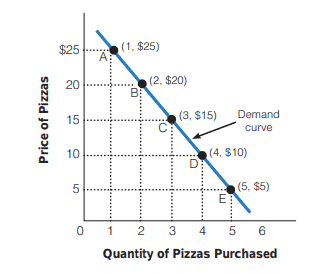
ThEach of us might want a nice home, two luxury cars, wholesome and good-tasting food, a personal trainer, and a therapist, all enjoyed in a pristine environment with zero pollution. If we had unlimited resources, and thus an ability to produce all the goods and services everyone wants, we would not have to choose among those desires. However, we all face scarcity, and as a consequence, we must make choices. If we did not have to make meaningful economic choices, the study of economics would not be necessary. The essence of economics is to understand fully the implications that scarcity has for wise decision making.

In a world of scarcity, we all face trade-offs. If you spend more time at work you might give up an opportunity to go shopping at the mall or watch your favorite television show. Time spent exercising means giving up something else that is valuable-perhaps relaxing with friends or studying for an upcoming exam. Or when you decide how to spend your income, buying a new car may mean you have to forgo a summer vacation. Businesses have tradeoffs, too. If a farmer chooses to plant his land in cotton this year, he gives up the opportunity to plant his land in wheat. If a firm decides to produce only cars, it gives up the opportunity to use those resources to produce refrigerators or something else that people value. Society, too, must make trade-offs. For example, the federal government faces trade-offs when it comes to spending tax revenues; additional resources used to enhance the environment may come at the expense of additional resources to provide health care, education, or national defense.

经济代写|宏观经济学代写Macroeconomics代考|To Choose Is to Lose

Every choice involves a cost. Anytime you are doing something, you could be doing something else. The next highest or best forgone opportunity resulting from a decision is called the opportunity cost. Another way to put it is that “to choose is to lose,” or, “An opportunity cost is the highest valued opportunity lost.” It is important to remember that the opportunity cost involves the next highest valued alternative, not all alternatives not chosen. For example, what would you have been doing with your time if you were not reading this book? Or what if you were planning on going to the gym to work out, and then your best friend calls and invites you to sit in his courtside seats at the Los Angeles Lakers game (your favorite team). What just happened to the cost of going to the gym? The next best alternative is what you give up, not all the things you could have been doing. To get more of anything that is desirable, you must accept less of something else that you also value. The higher the opportunity cost of doing something, the less likely it will be done. So if the opportunity cost of going to class increases relative to its benefit, you will be less likely to go to class.

Every choice you make has a cost, an opportunity cost. All productive resources have alternative uses regardless of who owns them-individuals, firms, or government. For example, if a city uses land for a new school, the cost is the next-best alternative use of that landperhaps, a park. To have a meaningful understanding of cost, you must be able to compare the alternative opportunities that are sacrificed in that choice.

Bill Gates, Tiger Woods, and Oprah Winfrey all quit college to pursue their dreams. Tiger Woods dropped out of Stanford (an economics major) to join the PGA golf tour. Bill Gates dropped out of Harvard to start a software company. Oprah Winfrey dropped out of Tennessee State to pursue a career in broadcasting. At the early age of 19 , she became the co-anchor of the evening news. LeBron James (Cleveland Cavaliers), Kobe Bryant (LA Lakers), and Alex Rodriguez (New York Yankees) understood opportunity cost; they didn’t even start college, and it worked out well for them. Staying in, or starting, college would have cost each of them millions of dollars. We cannot say it would have been the wrong decision to stay in or never start college, but it would have been costly. Their opportunity cost of staying in or going to or starting college was high.

宏观经济学代考

经济代写|宏观经济学代写Macroeconomics代考|Scarcity Forces Us to Choose

我们每个人可能都想要一个漂亮的家，两辆豪车，健康美味的食物，一个私人教练和一个治疗师，在一个零污染的原始环境中享受这一切。如果我们拥有无限的资源，从而有能力生产每个人想要的所有商品和服务，我们就不必在这些欲望中做出选择。然而，我们都面临着匮乏，因此，我们必须做出选择。如果我们不必做出有意义的经济选择，那么经济学的研究就没有必要了。经济学的本质是充分理解稀缺对明智决策的影响。

在一个资源匮乏的世界里，我们都面临着取舍。如果你花更多的时间在工作上，你可能会放弃去商场购物或看你最喜欢的电视节目的机会。花在锻炼上的时间意味着放弃其他有价值的事情——也许是和朋友一起放松，或者是为即将到来的考试学习。或者当你决定如何花费你的收入时，买一辆新车可能意味着你不得不放弃一个暑假。企业也有取舍。如果一个农民今年选择在他的土地上种棉花，他就放弃了在他的土地上种小麦的机会。如果一家公司决定只生产汽车，它就放弃了利用这些资源生产冰箱或其他人们看重的东西的机会。社会也必须做出取舍。例如，联邦政府在支出税收收入时面临权衡;用于改善环境的额外资源可能以牺牲用于提供卫生保健、教育或国防的额外资源为代价。

经济代写|宏观经济学代写Macroeconomics代考|To Choose Is to Lose

每一个选择都有代价。当你在做某件事的时候，你也可能在做别的事。由于决策而放弃的次高或最佳机会称为机会成本。另一种说法是“选择就是失去”，或者“机会成本是失去的最有价值的机会”。重要的是要记住，机会成本涉及下一个价值最高的选择，而不是所有没有选择的选择。例如，如果你没有读这本书，你会怎么打发时间呢?或者，如果你打算去健身房锻炼，然后你最好的朋友打来电话，邀请你坐在他的场边座位上看洛杉矶湖人队(你最喜欢的球队)的比赛。去健身房的费用怎么了?次佳选择是你放弃的东西，而不是你本来可以做的所有事情。为了得到更多你想要的东西，你必须少接受一些你同样看重的东西。做某件事的机会成本越高，就越不可能被完成。因此，如果上课的机会成本相对于收益增加，你就不太可能去上课。

你做的每一个选择都有成本，机会成本。所有的生产资源都有不同的用途，无论是个人、公司还是政府。例如，如果一个城市用土地建一所新学校，其成本是土地的次优用途——也许是公园。为了对成本有一个有意义的理解，你必须能够比较在这个选择中牺牲的其他机会。

比尔·盖茨、老虎·伍兹和奥普拉·温弗瑞都放弃了大学学业去追求自己的梦想。老虎伍兹从斯坦福大学(经济学专业)退学，参加了美国职业高尔夫球协会(PGA)巡回赛。比尔·盖茨从哈佛辍学，创办了一家软件公司。奥普拉·温弗瑞从田纳西州辍学，从事广播事业。19岁时，她就成为了晚间新闻的联合主播。勒布朗·詹姆斯(克利夫兰骑士)、科比·布莱恩特(洛杉矶湖人)和亚历克斯·罗德里格斯(纽约洋基)了解机会成本;他们甚至没有开始上大学，但这对他们来说很好。留在大学或开始上大学将花费他们每个人数百万美元。我们不能说留在大学或不上大学是错误的决定，但它会付出高昂的代价。他们上大学的机会成本很高。

统计代写请认准statistics-lab™. statistics-lab™为您的留学生涯保驾护航。

金融工程代写

金融工程是使用数学技术来解决金融问题。金融工程使用计算机科学、统计学、经济学和应用数学领域的工具和知识来解决当前的金融问题，以及设计新的和创新的金融产品。

非参数统计代写

非参数统计指的是一种统计方法，其中不假设数据来自于由少数参数决定的规定模型；这种模型的例子包括正态分布模型和线性回归模型。

广义线性模型代考

广义线性模型（GLM）归属统计学领域，是一种应用灵活的线性回归模型。该模型允许因变量的偏差分布有除了正态分布之外的其它分布。

术语 广义线性模型（GLM）通常是指给定连续和/或分类预测因素的连续响应变量的常规线性回归模型。它包括多元线性回归，以及方差分析和方差分析（仅含固定效应）。

有限元方法代写

有限元方法（FEM）是一种流行的方法，用于数值解决工程和数学建模中出现的微分方程。典型的问题领域包括结构分析、传热、流体流动、质量运输和电磁势等传统领域。

有限元是一种通用的数值方法，用于解决两个或三个空间变量的偏微分方程（即一些边界值问题）。为了解决一个问题，有限元将一个大系统细分为更小、更简单的部分，称为有限元。这是通过在空间维度上的特定空间离散化来实现的，它是通过构建对象的网格来实现的：用于求解的数值域，它有有限数量的点。边界值问题的有限元方法表述最终导致一个代数方程组。该方法在域上对未知函数进行逼近。[1] 然后将模拟这些有限元的简单方程组合成一个更大的方程系统，以模拟整个问题。然后，有限元通过变化微积分使相关的误差函数最小化来逼近一个解决方案。

tatistics-lab作为专业的留学生服务机构，多年来已为美国、英国、加拿大、澳洲等留学热门地的学生提供专业的学术服务，包括但不限于Essay代写，Assignment代写，Dissertation代写，Report代写，小组作业代写，Proposal代写，Paper代写，Presentation代写，计算机作业代写，论文修改和润色，网课代做，exam代考等等。写作范围涵盖高中，本科，研究生等海外留学全阶段，辐射金融，经济学，会计学，审计学，管理学等全球99%专业科目。写作团队既有专业英语母语作者，也有海外名校硕博留学生，每位写作老师都拥有过硬的语言能力，专业的学科背景和学术写作经验。我们承诺100%原创，100%专业，100%准时，100%满意。

随机分析代写

随机微积分是数学的一个分支，对随机过程进行操作。它允许为随机过程的积分定义一个关于随机过程的一致的积分理论。这个领域是由日本数学家伊藤清在第二次世界大战期间创建并开始的。

时间序列分析代写

随机过程，是依赖于参数的一组随机变量的全体，参数通常是时间。 随机变量是随机现象的数量表现，其时间序列是一组按照时间发生先后顺序进行排列的数据点序列。通常一组时间序列的时间间隔为一恒定值（如1秒，5分钟，12小时，7天，1年），因此时间序列可以作为离散时间数据进行分析处理。研究时间序列数据的意义在于现实中，往往需要研究某个事物其随时间发展变化的规律。这就需要通过研究该事物过去发展的历史记录，以得到其自身发展的规律。

回归分析代写

多元回归分析渐进（Multiple Regression Analysis Asymptotics）属于计量经济学领域，主要是一种数学上的统计分析方法，可以分析复杂情况下各影响因素的数学关系，在自然科学、社会和经济学等多个领域内应用广泛。

MATLAB代写

MATLAB 是一种用于技术计算的高性能语言。它将计算、可视化和编程集成在一个易于使用的环境中，其中问题和解决方案以熟悉的数学符号表示。典型用途包括：数学和计算算法开发建模、仿真和原型制作数据分析、探索和可视化科学和工程图形应用程序开发，包括图形用户界面构建MATLAB 是一个交互式系统，其基本数据元素是一个不需要维度的数组。这使您可以解决许多技术计算问题，尤其是那些具有矩阵和向量公式的问题，而只需用 C 或 Fortran 等标量非交互式语言编写程序所需的时间的一小部分。MATLAB 名称代表矩阵实验室。MATLAB 最初的编写目的是提供对由 LINPACK 和 EISPACK 项目开发的矩阵软件的轻松访问，这两个项目共同代表了矩阵计算软件的最新技术。MATLAB 经过多年的发展，得到了许多用户的投入。在大学环境中，它是数学、工程和科学入门和高级课程的标准教学工具。在工业领域，MATLAB 是高效研究、开发和分析的首选工具。MATLAB 具有一系列称为工具箱的特定于应用程序的解决方案。对于大多数 MATLAB 用户来说非常重要，工具箱允许您学习和应用专业技术。工具箱是 MATLAB 函数（M 文件）的综合集合，可扩展 MATLAB 环境以解决特定类别的问题。可用工具箱的领域包括信号处理、控制系统、神经网络、模糊逻辑、小波、仿真等。

R语言代写	问卷设计与分析代写
PYTHON代写	回归分析与线性模型代写
MATLAB代写	方差分析与试验设计代写
STATA代写	机器学习/统计学习代写
SPSS代写	计量经济学代写
EVIEWS代写	时间序列分析代写
EXCEL代写	深度学习代写
SQL代写	各种数据建模与可视化代写

如果你也在 怎样代写宏观经济学Macroeconomics 这个学科遇到相关的难题，请随时右上角联系我们的24/7代写客服。宏观经济学Macroeconomics对国家或地区经济整体行为的研究。它关注的是对整个经济事件的理解，如商品和服务的生产总量、失业水平和价格的一般行为。宏观经济学关注的是经济体的表现–经济产出、通货膨胀、利率和外汇兑换率以及国际收支的变化。减贫、社会公平和可持续增长只有在健全的货币和财政政策下才能实现。

宏观经济学Macroeconomics（来自希腊语前缀makro-，意思是 “大 “+经济学）是经济学的一个分支，处理整个经济体的表现、结构、行为和决策。例如，使用利率、税收和政府支出来调节经济的增长和稳定。这包括区域、国家和全球经济。根据经济学家Emi Nakamura和Jón Steinsson在2018年的评估，经济 “关于不同宏观经济政策的后果的证据仍然非常不完善，并受到严重批评。宏观经济学家研究的主题包括GDP（国内生产总值）、失业（包括失业率）、国民收入、价格指数、产出、消费、通货膨胀、储蓄、投资、能源、国际贸易和国际金融。

statistics-lab™ 为您的留学生涯保驾护航 在代写宏观经济学Macroeconomics方面已经树立了自己的口碑, 保证靠谱, 高质且原创的统计Statistics代写服务。我们的专家在代写宏观经济学Macroeconomics代写方面经验极为丰富，各种代写宏观经济学Macroeconomics相关的作业也就用不着说。

经济代写|宏观经济学代写Macroeconomics代考|Positive versus Normative Analysis

The distinction between positive and normative analysis is important. It is one thing to say that everyone should have universal health care, an untestable normative statement, and quite another to say that universal health care would lead to greater worker productivity, a testable positive statement. It is important to distinguish between positive and normative analysis because many controversies in economics revolve around policy considerations that contain both. For example, what impact would a 3 percent reduction in income taxes across the board have on the economy? This question requires positive analysis. Whether we should have a 3 percent reduction in income taxes requires normative analysis as well. When economists are trying to explain the way the world works, they are scientists. When economists start talking about how the economy should work rather than how it does work, they have entered the normative world of the policy maker. Anytime you see the word should, that is a sign you are in the realm of normative economics. Positive statements are about what is, normative statements are about what ought to or should be. In short, positive statements are attempts to describe what happens and why it happens, while normative statements are attempts to prescribe what should be done. But sometimes the two are intertwined. For example, there are two different types of policies that are used to help low-income housing residents: rent controls, which control how much rent a landlord can charge, and rent subsidies, which provide low-income families with money to pay rent. While both are policies that engage normative analysis, most economists would favor the subsidy because it is more efficient – a conclusion derived from positive analysis.

经济代写|宏观经济学代写Macroeconomics代考|Disagreement Is Common in Most Disciplines

Although economists do frequently have opposing views on economic policy questions, they probably disagree less than the media would have you believe. Disagreement is common in most disciplines: Seismologists differ over predictions of earthquakes or volcanic eruption; historians can be at odds over the interpretation of historical events; psychologists disagree on proper ways to raise children; and nutritionists debate the efficacy of particular vitamins and the quantities that should be taken.

The majority of disagreements in economics stem from normative issues; differences in values or policy beliefs result in conflict. For example, a policy might increase efficiency at the expense of a sense of fairness or equity, or it might help a current generation at the expense of a future generation. Because policy decisions involve trade-offs, they will always involve the potential for conflict.

Some economists are concerned about individual freedom and liberty, thinking that any encroachment on individual decision making is bad, other things being equal. People with this philosophic bent are inclined to be skeptical of any increased government involvement in the economy.

On the other hand, some economists are concerned with what they consider an unequal, “unfair,” or unfortunate distribution of income, wealth, or power, and view governmental intervention as desirable in righting injustices that they believe exist in a market economy. To these persons, the threat to individual liberty alone is not sufficient to reject governmental intervention in the face of perceived economic injustice.

宏观经济学代考

经济代写|宏观经济学代写Macroeconomics代考|Positive versus Normative Analysis

实证分析和规范分析之间的区别很重要。说每个人都应该享有全民医疗保健是一回事，这是一个无法检验的规范性陈述;说全民医疗保健将导致更高的工人生产率是另一回事，这是一个可检验的积极陈述。区分积极分析和规范分析是很重要的，因为经济学中的许多争议都围绕着包含这两种分析的政策考虑。例如，全面减少3%的所得税会对经济产生什么影响?这个问题需要积极的分析。我们是否应该减少3%的所得税也需要规范分析。当经济学家试图解释世界运行的方式时，他们是科学家。当经济学家开始谈论经济应该如何运行，而不是经济如何运行时，他们就进入了政策制定者的规范世界。只要你看到“应该”这个词，那就表明你已经进入了规范经济学的领域。肯定陈述是关于“是什么”，规范陈述是关于“应该是什么”。简而言之，肯定陈述句试图描述发生了什么以及为什么会发生，而规范性陈述句试图规定应该做什么。但有时这两者是交织在一起的。例如，有两种不同类型的政策用于帮助低收入住房居民:租金管制，控制房东可以收取多少租金，以及租金补贴，为低收入家庭提供支付租金的资金。虽然这两种政策都需要进行规范分析，但大多数经济学家会支持补贴，因为它更有效——这是一个来自实证分析的结论。

经济代写|宏观经济学代写Macroeconomics代考|Disagreement Is Common in Most Disciplines

尽管经济学家确实经常在经济政策问题上持相反的观点，但他们的分歧可能比媒体让你相信的要少。分歧在大多数学科中都很常见:地震学家对地震或火山爆发的预测存在分歧;历史学家对历史事件的解释可能存在分歧;心理学家对养育孩子的正确方法意见不一;营养学家对某些维生素的功效和应该服用的量争论不休。

经济学中的大多数分歧源于规范问题;价值观或政策信仰的差异会导致冲突。例如，一项政策可能会以牺牲公平或公平感为代价来提高效率，或者以牺牲后代为代价来帮助当代人。因为政策决策涉及权衡，它们总是会涉及潜在的冲突。

一些经济学家担心个人自由和自由，认为在其他条件相同的情况下，任何对个人决策的侵犯都是不好的。有这种哲学倾向的人倾向于怀疑政府对经济的任何进一步干预。

另一方面，一些经济学家关注他们所认为的不平等、“不公平”或不幸的收入、财富或权力分配，并认为政府干预是纠正他们认为存在于市场经济中的不公正的可取之处。对这些人来说，对个人自由的威胁本身并不足以使他们在面对经济不公正时拒绝政府的干预。

统计代写请认准statistics-lab™. statistics-lab™为您的留学生涯保驾护航。

金融工程代写

金融工程是使用数学技术来解决金融问题。金融工程使用计算机科学、统计学、经济学和应用数学领域的工具和知识来解决当前的金融问题，以及设计新的和创新的金融产品。

非参数统计代写

非参数统计指的是一种统计方法，其中不假设数据来自于由少数参数决定的规定模型；这种模型的例子包括正态分布模型和线性回归模型。

广义线性模型代考

广义线性模型（GLM）归属统计学领域，是一种应用灵活的线性回归模型。该模型允许因变量的偏差分布有除了正态分布之外的其它分布。

术语 广义线性模型（GLM）通常是指给定连续和/或分类预测因素的连续响应变量的常规线性回归模型。它包括多元线性回归，以及方差分析和方差分析（仅含固定效应）。

有限元方法代写

有限元方法（FEM）是一种流行的方法，用于数值解决工程和数学建模中出现的微分方程。典型的问题领域包括结构分析、传热、流体流动、质量运输和电磁势等传统领域。

有限元是一种通用的数值方法，用于解决两个或三个空间变量的偏微分方程（即一些边界值问题）。为了解决一个问题，有限元将一个大系统细分为更小、更简单的部分，称为有限元。这是通过在空间维度上的特定空间离散化来实现的，它是通过构建对象的网格来实现的：用于求解的数值域，它有有限数量的点。边界值问题的有限元方法表述最终导致一个代数方程组。该方法在域上对未知函数进行逼近。[1] 然后将模拟这些有限元的简单方程组合成一个更大的方程系统，以模拟整个问题。然后，有限元通过变化微积分使相关的误差函数最小化来逼近一个解决方案。

tatistics-lab作为专业的留学生服务机构，多年来已为美国、英国、加拿大、澳洲等留学热门地的学生提供专业的学术服务，包括但不限于Essay代写，Assignment代写，Dissertation代写，Report代写，小组作业代写，Proposal代写，Paper代写，Presentation代写，计算机作业代写，论文修改和润色，网课代做，exam代考等等。写作范围涵盖高中，本科，研究生等海外留学全阶段，辐射金融，经济学，会计学，审计学，管理学等全球99%专业科目。写作团队既有专业英语母语作者，也有海外名校硕博留学生，每位写作老师都拥有过硬的语言能力，专业的学科背景和学术写作经验。我们承诺100%原创，100%专业，100%准时，100%满意。

随机分析代写

随机微积分是数学的一个分支，对随机过程进行操作。它允许为随机过程的积分定义一个关于随机过程的一致的积分理论。这个领域是由日本数学家伊藤清在第二次世界大战期间创建并开始的。

时间序列分析代写

随机过程，是依赖于参数的一组随机变量的全体，参数通常是时间。 随机变量是随机现象的数量表现，其时间序列是一组按照时间发生先后顺序进行排列的数据点序列。通常一组时间序列的时间间隔为一恒定值（如1秒，5分钟，12小时，7天，1年），因此时间序列可以作为离散时间数据进行分析处理。研究时间序列数据的意义在于现实中，往往需要研究某个事物其随时间发展变化的规律。这就需要通过研究该事物过去发展的历史记录，以得到其自身发展的规律。

回归分析代写

多元回归分析渐进（Multiple Regression Analysis Asymptotics）属于计量经济学领域，主要是一种数学上的统计分析方法，可以分析复杂情况下各影响因素的数学关系，在自然科学、社会和经济学等多个领域内应用广泛。

MATLAB代写

MATLAB 是一种用于技术计算的高性能语言。它将计算、可视化和编程集成在一个易于使用的环境中，其中问题和解决方案以熟悉的数学符号表示。典型用途包括：数学和计算算法开发建模、仿真和原型制作数据分析、探索和可视化科学和工程图形应用程序开发，包括图形用户界面构建MATLAB 是一个交互式系统，其基本数据元素是一个不需要维度的数组。这使您可以解决许多技术计算问题，尤其是那些具有矩阵和向量公式的问题，而只需用 C 或 Fortran 等标量非交互式语言编写程序所需的时间的一小部分。MATLAB 名称代表矩阵实验室。MATLAB 最初的编写目的是提供对由 LINPACK 和 EISPACK 项目开发的矩阵软件的轻松访问，这两个项目共同代表了矩阵计算软件的最新技术。MATLAB 经过多年的发展，得到了许多用户的投入。在大学环境中，它是数学、工程和科学入门和高级课程的标准教学工具。在工业领域，MATLAB 是高效研究、开发和分析的首选工具。MATLAB 具有一系列称为工具箱的特定于应用程序的解决方案。对于大多数 MATLAB 用户来说非常重要，工具箱允许您学习和应用专业技术。工具箱是 MATLAB 函数（M 文件）的综合集合，可扩展 MATLAB 环境以解决特定类别的问题。可用工具箱的领域包括信号处理、控制系统、神经网络、模糊逻辑、小波、仿真等。

R语言代写	问卷设计与分析代写
PYTHON代写	回归分析与线性模型代写
MATLAB代写	方差分析与试验设计代写
STATA代写	机器学习/统计学习代写
SPSS代写	计量经济学代写
EVIEWS代写	时间序列分析代写
EXCEL代写	深度学习代写
SQL代写	各种数据建模与可视化代写

如果你也在 怎样代写宏观经济学Macroeconomics 这个学科遇到相关的难题，请随时右上角联系我们的24/7代写客服。宏观经济学Macroeconomics对国家或地区经济整体行为的研究。它关注的是对整个经济事件的理解，如商品和服务的生产总量、失业水平和价格的一般行为。宏观经济学关注的是经济体的表现–经济产出、通货膨胀、利率和外汇兑换率以及国际收支的变化。减贫、社会公平和可持续增长只有在健全的货币和财政政策下才能实现。

宏观经济学Macroeconomics（来自希腊语前缀makro-，意思是 “大 “+经济学）是经济学的一个分支，处理整个经济体的表现、结构、行为和决策。例如，使用利率、税收和政府支出来调节经济的增长和稳定。这包括区域、国家和全球经济。根据经济学家Emi Nakamura和Jón Steinsson在2018年的评估，经济 “关于不同宏观经济政策的后果的证据仍然非常不完善，并受到严重批评。宏观经济学家研究的主题包括GDP（国内生产总值）、失业（包括失业率）、国民收入、价格指数、产出、消费、通货膨胀、储蓄、投资、能源、国际贸易和国际金融。

statistics-lab™ 为您的留学生涯保驾护航 在代写宏观经济学Macroeconomics方面已经树立了自己的口碑, 保证靠谱, 高质且原创的统计Statistics代写服务。我们的专家在代写宏观经济学Macroeconomics代写方面经验极为丰富，各种代写宏观经济学Macroeconomics相关的作业也就用不着说。

经济代写|宏观经济学代写Macroeconomics代考|Science and Stories

Much of scientific discovery is expressed in terms of stories, not unlike the stories told by novelists. This similarity is not accidental. The novelist tries to persuade us that a story could almost be true; the scientist tries to persuade us that certain events fall into a certain meaningful pattern. The scientist does not (or is not supposed to) invent the underlying “facts” of the story, whereas the novelist is not so constrained. However, a scientist does select certain facts from among many facts that could have been chosen, just as the novelist chooses from an infinite number of possible characters and situations to make the story most persuasive. In both cases, the author “invents” the story. Therefore, we should not be surprised to find order in economic theory any more than we are surprised to find order in a good novel. Scientists would not bother to write about “life” if they were not convinced that they had stories worth telling.
What makes a story “worth telling”? When we look for order in nature, we cannot suppose that the “facts” are a sufficient basis for understanding observed events. The basic problem is that the facts of a complex world simply do not organize themselves. Understanding requires that a conceptual order be imposed on these “facts” to counteract the confusion that would otherwise result. For example, objects of different weights falling freely in the air do not travel at precisely the same rate (largely because of the different effects of air resistance). Yet this piece of information is generally much less significant than the fact that falling bodies do travel at almost the same rate (which presumably would be identical in a vacuum). By focusing on the most significant fact-the similarity, not the difference-Galileo was able to impose order on the story of gravity.

In the same way, to interpret the impact of rising housing prices on the amount of housing desired, economists must separate out the impact of increasing wealth, population, and other contributing factors. Failing to do so would obscure the central insight that people tend to buy less housing at higher prices. Without a story – a theory of causation-scientists could not sort out and understand the complex reality that surrounds us.

经济代写|宏观经济学代写Macroeconomics代考|The Ceteris Paribus Assumption

Virtually all economic theories share a condition usually expressed by the Latin phrase ceteris paribus. A rough translation of the phrase is “letting everything else be equal” or “holding everything else constant.” When economists try to assess the effect of one variable on another, they must keep the relationship between the two variables isolated from other events that might also influence the situation that the theory tries to explain or predict. In other words, everything else freezes so we can see how one thing affects another. For example, if the price of tomatoes falls, we would expect to see more people buy tomatoes. But if the government recently recommended not buying tomatoes because they have been infected by a bug that causes intestinal problems, people would buy fewer, not more, at lower prices. Does that mean you throw out your theory that people buy more at lower prices? No, we just did not freeze the effects of news from the government, which had a greater impact on purchases than lower prices did. Let’s return to the gravity example. Suppose you drop a feather and a brick off the Eiffel Tower on a windy day. We would expect the brick to win the race. But if we could hold everything constant in a vacuum, then we would expect them to hit the ground at the same time. The law of gravity needs the ceteris paribus assumption, too.

宏观经济学代考

经济代写|宏观经济学代写Macroeconomics代考|Science and Stories

许多科学发现都是用故事来表达的，就像小说家讲的故事一样。这种相似性并非偶然。小说家试图让我们相信，一个故事可能几乎是真的;科学家试图说服我们，某些事件符合某种有意义的模式。科学家不会(或不应该)发明故事的潜在“事实”，而小说家则不受此限制。然而，科学家确实从许多可以选择的事实中选择了某些事实，就像小说家从无数可能的人物和情景中选择一样，使故事最具说服力。在这两种情况下，作者都“虚构”了故事。因此，我们不应该惊讶于在经济理论中发现秩序，正如我们不应该惊讶于在一本好小说中发现秩序一样。如果科学家们不相信他们有值得讲述的故事，他们是不会费心去写“生命”的。
是什么让一个故事“值得讲述”?当我们寻找自然界的秩序时，我们不能假设“事实”是理解观察到的事件的充分基础。基本的问题是，一个复杂世界的事实本身并没有组织起来。理解需要对这些“事实”施加一个概念上的秩序，以抵消否则可能导致的混乱。例如，在空气中自由下落的不同重量的物体并不以完全相同的速度运动(主要是因为空气阻力的不同影响)。然而，与落体以几乎相同的速度运动(这在真空中可能是相同的)这一事实相比，这条信息的重要性要小得多。通过关注最重要的事实——相似性，而不是差异——伽利略能够给引力的故事强加秩序。

同样，为了解释房价上涨对住房需求数量的影响，经济学家必须分离出财富增长、人口增长和其他因素的影响。如果不这样做，人们往往会在更高的价格下购买更少的住房，这一核心观点就会变得模糊。没有故事——没有因果关系理论——科学家就无法理清和理解我们周围复杂的现实。

经济代写|宏观经济学代写Macroeconomics代考|The Ceteris Paribus Assumption

实际上，所有的经济理论都有一个共同的条件，这个条件通常用拉丁短语“其他条件相同”来表达。这个短语的粗略翻译是“让其他一切都平等”或“保持其他一切不变”。当经济学家试图评估一个变量对另一个变量的影响时，他们必须将两个变量之间的关系与其他事件隔离开来，这些事件也可能影响该理论试图解释或预测的情况。换句话说，其他一切都冻结了，这样我们就可以看到一件事是如何影响另一件事的。例如，如果西红柿的价格下跌，我们预计会看到更多的人购买西红柿。但是，如果政府最近建议不要购买西红柿，因为它们感染了一种会导致肠道问题的细菌，人们就会以更低的价格购买更少而不是更多的西红柿。这是否意味着你要抛弃人们在更低价格下买得更多的理论?不，我们只是没有冻结来自政府的消息的影响，这对购买的影响比低价格的影响更大。让我们回到重力的例子。假设你在一个刮风的日子从埃菲尔铁塔上掉下一根羽毛和一块砖头。我们认为砖头会赢得比赛。但如果我们能在真空中保持所有东西不变，那么我们就能预期它们同时落地。万有引力定律也需要“地中心”的假设。

统计代写请认准statistics-lab™. statistics-lab™为您的留学生涯保驾护航。

金融工程代写

金融工程是使用数学技术来解决金融问题。金融工程使用计算机科学、统计学、经济学和应用数学领域的工具和知识来解决当前的金融问题，以及设计新的和创新的金融产品。

非参数统计代写

非参数统计指的是一种统计方法，其中不假设数据来自于由少数参数决定的规定模型；这种模型的例子包括正态分布模型和线性回归模型。

广义线性模型代考

广义线性模型（GLM）归属统计学领域，是一种应用灵活的线性回归模型。该模型允许因变量的偏差分布有除了正态分布之外的其它分布。

术语 广义线性模型（GLM）通常是指给定连续和/或分类预测因素的连续响应变量的常规线性回归模型。它包括多元线性回归，以及方差分析和方差分析（仅含固定效应）。

有限元方法代写

有限元方法（FEM）是一种流行的方法，用于数值解决工程和数学建模中出现的微分方程。典型的问题领域包括结构分析、传热、流体流动、质量运输和电磁势等传统领域。

有限元是一种通用的数值方法，用于解决两个或三个空间变量的偏微分方程（即一些边界值问题）。为了解决一个问题，有限元将一个大系统细分为更小、更简单的部分，称为有限元。这是通过在空间维度上的特定空间离散化来实现的，它是通过构建对象的网格来实现的：用于求解的数值域，它有有限数量的点。边界值问题的有限元方法表述最终导致一个代数方程组。该方法在域上对未知函数进行逼近。[1] 然后将模拟这些有限元的简单方程组合成一个更大的方程系统，以模拟整个问题。然后，有限元通过变化微积分使相关的误差函数最小化来逼近一个解决方案。

tatistics-lab作为专业的留学生服务机构，多年来已为美国、英国、加拿大、澳洲等留学热门地的学生提供专业的学术服务，包括但不限于Essay代写，Assignment代写，Dissertation代写，Report代写，小组作业代写，Proposal代写，Paper代写，Presentation代写，计算机作业代写，论文修改和润色，网课代做，exam代考等等。写作范围涵盖高中，本科，研究生等海外留学全阶段，辐射金融，经济学，会计学，审计学，管理学等全球99%专业科目。写作团队既有专业英语母语作者，也有海外名校硕博留学生，每位写作老师都拥有过硬的语言能力，专业的学科背景和学术写作经验。我们承诺100%原创，100%专业，100%准时，100%满意。

随机分析代写

随机微积分是数学的一个分支，对随机过程进行操作。它允许为随机过程的积分定义一个关于随机过程的一致的积分理论。这个领域是由日本数学家伊藤清在第二次世界大战期间创建并开始的。

时间序列分析代写

随机过程，是依赖于参数的一组随机变量的全体，参数通常是时间。 随机变量是随机现象的数量表现，其时间序列是一组按照时间发生先后顺序进行排列的数据点序列。通常一组时间序列的时间间隔为一恒定值（如1秒，5分钟，12小时，7天，1年），因此时间序列可以作为离散时间数据进行分析处理。研究时间序列数据的意义在于现实中，往往需要研究某个事物其随时间发展变化的规律。这就需要通过研究该事物过去发展的历史记录，以得到其自身发展的规律。

回归分析代写

多元回归分析渐进（Multiple Regression Analysis Asymptotics）属于计量经济学领域，主要是一种数学上的统计分析方法，可以分析复杂情况下各影响因素的数学关系，在自然科学、社会和经济学等多个领域内应用广泛。

MATLAB代写

MATLAB 是一种用于技术计算的高性能语言。它将计算、可视化和编程集成在一个易于使用的环境中，其中问题和解决方案以熟悉的数学符号表示。典型用途包括：数学和计算算法开发建模、仿真和原型制作数据分析、探索和可视化科学和工程图形应用程序开发，包括图形用户界面构建MATLAB 是一个交互式系统，其基本数据元素是一个不需要维度的数组。这使您可以解决许多技术计算问题，尤其是那些具有矩阵和向量公式的问题，而只需用 C 或 Fortran 等标量非交互式语言编写程序所需的时间的一小部分。MATLAB 名称代表矩阵实验室。MATLAB 最初的编写目的是提供对由 LINPACK 和 EISPACK 项目开发的矩阵软件的轻松访问，这两个项目共同代表了矩阵计算软件的最新技术。MATLAB 经过多年的发展，得到了许多用户的投入。在大学环境中，它是数学、工程和科学入门和高级课程的标准教学工具。在工业领域，MATLAB 是高效研究、开发和分析的首选工具。MATLAB 具有一系列称为工具箱的特定于应用程序的解决方案。对于大多数 MATLAB 用户来说非常重要，工具箱允许您学习和应用专业技术。工具箱是 MATLAB 函数（M 文件）的综合集合，可扩展 MATLAB 环境以解决特定类别的问题。可用工具箱的领域包括信号处理、控制系统、神经网络、模糊逻辑、小波、仿真等。

R语言代写	问卷设计与分析代写
PYTHON代写	回归分析与线性模型代写
MATLAB代写	方差分析与试验设计代写
STATA代写	机器学习/统计学习代写
SPSS代写	计量经济学代写
EVIEWS代写	时间序列分析代写
EXCEL代写	深度学习代写
SQL代写	各种数据建模与可视化代写

如果你也在 怎样代写宏观经济学Macroeconomics这个学科遇到相关的难题，请随时右上角联系我们的24/7代写客服。

宏观经济学，对国家或地区经济整体行为的研究。它关注的是了解整个经济的事件，如商品和服务的生产总量、失业水平和价格的一般行为。

statistics-lab™ 为您的留学生涯保驾护航 在代写宏观经济学Macroeconomics方面已经树立了自己的口碑, 保证靠谱, 高质且原创的统计Statistics代写服务。我们的专家在代写宏观经济学Macroeconomics代写方面经验极为丰富，各种代写宏观经济学Macroeconomics相关的作业也就用不着说。

我们提供的宏观经济学Macroeconomics及其相关学科的代写，服务范围广, 其中包括但不限于:

• Statistical Inference 统计推断
• Statistical Computing 统计计算
• Advanced Probability Theory 高等概率论
• Advanced Mathematical Statistics 高等数理统计学
• (Generalized) Linear Models 广义线性模型
• Statistical Machine Learning 统计机器学习
• Longitudinal Data Analysis 纵向数据分析
• Foundations of Data Science 数据科学基础

经济代写|宏观经济学代写Macroeconomics代考|Supply Lags and Market Movements

Tinbergen proposed a supply lag scheme as early as 1928 , in a paper published in $D e$ Socialistische Gids. The paper was rather long considering that the journal usually published articles of only a dozen pages, and most of it was concerned with problems of exchange related to Cournot’s theories of competition. Incidentally, Tinbergen deplored the fact that Cournot’s work had remained mostly ignored, adding that the mathematical form in which it was published (in 1838) was probably to blame for this (Tinbergen, 1928: 543). ${ }^{14}$

The last part of this paper was concerned with the problem of the temporal element in his analysis, recognizing that this influence was mostly ignored in the previous sections. Tinbergen studied a problem of fluctuations around an equilibrium and based his discussion on a mechanical analogy: solving the “dynamic problem” meant that “as in mechanical dynamics, further data is needed, data which we can denote by inertia and delay, the inertia being related to the effort, the delay to the time of displacement” (Tinbergen, 1928: 544). Tinbergen then proposed to observe the behavior of one market where supply would adjust with a lag, while “demand adapts to supply without delay” (Tinbergen, 1928: 544). Although he did not explicitly present the equations behind his scheme, he did propose a numerical example with a figure of the temporal evolution of the quantities exchanged of a good, which took the form of damped oscillations that were in fact the result of a cobweb mechanism (reproduced in Fig. 2.2).of unstable equilibrium),” but he added that these fluctuations could occur “only occasionally” (Tinbergen, 1928: 547).

At the very end of his article, Tinbergen concluded with a reference to another work: “a very fine example of an isolated fluctuating market (with a period of 3-4 years) is that of the … pigs!”‘ (Tinbergen, 1928: 547). He was referring here to the work of Arthur Hanau on the cycles in the pig market that had just been published in the Vierteljahreshefte zur Konjunkturforschung, the journal of the Berlin Business Cycle Institute where Hanau was working at the time. Tinbergen would refer to this work enthusiastically many times afterward; its empirical conclusions clearly showed the importance of introducing lags and considering the dynamics of supply and demand on a market, and almost sixty years later he still gave credit to Hanau for the discovery of the mechanism of the supply lag (Tinbergen et al., 1987: 120). ${ }^{16}$
Even though the years after must have seen him busy writing his thesis about minimum problems, far from the lag problems studied here, Tinbergen’s work on this problem did not stop there. In fact, other works on the questions were being published simultaneously and independently of European economists. In the USA, Henry Moore had proposed as early as 1925 an analysis of the demand and supply of potatoes in the USA, where he introduced an implicit lag in supply which allowed him to estimate on the same data both his supply and his demand curve (Moore, 1925). This paper was reproduced in his 1929 book, Synthetic Economics, which had a wide circulation and was discussed by many American and European economists. ${ }^{17}$

经济代写|宏观经济学代写Macroeconomics代考|The Shipbuilding Model and Mixed Equations

In the introduction of his 1931 paper “Ein Problem der Dynamik,” when Tinbergen distinguished several lines of research that expanded “the static theory of social economy,” he finished his review by remarking that no one had yet tried to combine time derivatives and lags into a “systematic design of the dynamic theory” (Tinbergen, 1931a: 169). A scheme was proposed in the paper but it was still floundering; nevertheless, that same year, Tinbergen proposed a straightforward combination of time derivatives and lags, through his model of the shipbuilding cycle.

The choice of shipbuilding was not anecdotal; in a paper published in De Nederlandsche Conjunctuur, the journal of the Centraal Bureau voor de Statistiek (CBS) where he was working at the time, Tinbergen explained that “[t]he branch of industry concerned with shipbuilding has a number of peculiarities which make a study of the relationship between the business cycle and this branch of industry of great importance, especially for shipbuilding itself and for shipping companies” (Tinbergen, $1931 \mathrm{c}:$ 14). Shipbuilding was one of the biggest branches of activity in the Netherlands, and Tinbergen saw at least three characteristics that made its study worthwhile: the long production process of building ships, the strong fluctuations in its activity, and the long life of its means of production. This meant that the shipbuilding industry was quite different from the agricultural markets that had spurred the cobweb models of Moore, Schultz, Ricci and Tinbergen. Clearly, trying to explain the fluctuations of a market of durable instead of perishable goods led Tinbergen to important new ideas.

The first study that he published on the question (Tinbergen, 1931c) was very empirical as he tried to determine the lifespan of ships and other characteristics of the cycle. Nevertheless, he was also clearly searching for an explanation of the cycle, for a mechanism that would explain the fluctuations he had found empirically. He argued that a causal mechanism existed in particular between tonnage and its own increase: “[t]here is indeed a clear interaction between tonnage and increase in tonnage, an interaction which will be referred to in the remainder of this article as the ‘own mechanism’ of the development of tonnage” (Tinbergen, 1931c: 17). But he did not try in this paper to give a more mathematical form to this finding, which he reserved for a paper written in German for the Weltwirtschaftliches Archiv, the journal of the Kiel group of economists (Tinbergen 1931b, which was translated in Tinbergen 1959 from which we quote hereafter). ${ }^{24}$

Characteristically, Tinbergen started this second paper on shipbuilding with a nod to Moore and Hanau, hinting that this study was similar in character. But although it was concerned with fluctuations as well, the form he gave to his model was rather different than the simple cobweb, and most of the paper was concerned with the detailed presentation of Tinbergen’s solution of an equation of the type $\dot{f}(t)=-a f(t-\theta)$, which states that the time derivative of tonnage $\dot{f}$ is inversely proportional to the total tonnage a time $\theta$ ago (taken to be two years in his second paper). Although this is the simplest type of mixed differential-difference equations, it still poses some challenges to solve and Tinbergen’s background in theoretical physics served him well to work out an answer. Indeed this class of equations had not yet been studied extensively, and the absence of a road map to solve dynamic systems relying on them hindered the early development of macro-dynamic models, eventually leading to the abandonment of this approach in favor of simpler difference equations models in the late $1930 \mathrm{~s}$.

宏观经济学代考

经济代写|宏观经济学代写Macroeconomics代考|Supply Lags and Market Movements

Tinbergen 早在 1928 年就在一篇发表于丁这是Socialistische Gids。考虑到该杂志通常发表的文章通常只有十几页，而且大部分都是与古诺竞争理论相关的交流问题，所以这篇论文相当长。顺便说一句，Tinbergen 对古诺的工作几乎一直被忽视这一事实感到遗憾，并补充说它出版时所用的数学形式（1838 年）可能是造成这种情况的原因（Tinbergen，1928：543）。14

本文的最后一部分在他的分析中关注时间因素的问题，认识到这种影响在前几节中大多被忽略了。丁伯根研究了围绕平衡的波动问题，并将他的讨论基于机械类比：解决“动态问题”意味着“在机械动力学中，需要更多数据，我们可以用惯性和延迟表示的数据，惯性是与努力有关，延迟与流离失所的时间有关”（Tinbergen，1928：544）。Tinbergen 随后提议观察一个市场的行为，在该市场中，供应会滞后调整，而“需求会立即适应供应”（Tinbergen，1928：544）。尽管他没有明确提出他的方案背后的方程式，

在文章的最后，Tinbergen 引用了另一部著作得出结论：“孤立波动市场（周期为 3-4 年）的一个很好的例子是……猪！”（Tinbergen，1928 年） : 547). 他在这里指的是亚瑟·哈瑙 (Arthur Hanau) 关于猪市周期的著作，该著作刚刚发表在柏林商业周期研究所 (Berlin Business Cycle Institute) 的期刊 Vierteljahreshefte zur Konjunkturforschung 上，哈瑙当时正在该研究所工作。之后丁伯根多次热情地提到这部作品；它的实证结论清楚地表明引入滞后和考虑市场供求动态的重要性，将近 60 年后，他仍然相信哈瑙发现了供应滞后机制（Tinbergen 等人，1987 年） ：120）。16
尽管此后的几年里肯定看到他忙于撰写关于最小化问题的论文，但与这里研究的滞后问题相去甚远，丁伯根在这个问题上的工作并没有就此止步。事实上，关于这些问题的其他著作正在同时独立于欧洲经济学家出版。在美国，Henry Moore 早在 1925 年就提出了对美国马铃薯供需的分析，他在其中引入了隐含的供应滞后，这使他能够根据相同的数据估计他的供应和需求曲线（摩尔，1925 年）。这篇论文被转载于他 1929 年出版的《综合经济学》一书中，该书发行广泛，被许多欧美经济学家讨论过。17

经济代写|宏观经济学代写Macroeconomics代考|The Shipbuilding Model and Mixed Equations

在他 1931 年的论文“Ein Problem der Dynamik”的引言中，当 Tinbergen 区分了扩展“社会经济的静态理论”的几条研究路线时，他在结束评论时说，还没有人试图将时间导数和滞后结合起来进入“动态理论的系统设计”（Tinbergen，1931a：169）。论文中提出了一个方案，但仍在挣扎；尽管如此，同年，丁伯根通过他的造船周期模型提出了时间导数和滞后的直接组合。

造船的选择不是轶事。在他当时工作的中央统计局 (CBS) 期刊 De Nederlandsche Conjunctuur 上发表的一篇论文中，Tinbergen 解释说，“与造船业有关的行业有许多特点，这使得研究商业周期与这个非常重要的行业分支之间的关系，特别是对于造船业本身和航运公司”（Tinbergen，1931C:14). 造船业是荷兰最大的活动分支之一，丁伯根至少看到了三个值得研究的特点：造船的生产过程漫长、活动波动剧烈，以及生产资料的使用寿命长. 这意味着造船业与刺激了摩尔、舒尔茨、里奇和丁伯根蜘蛛网模型的农业市场截然不同。显然，试图解释耐用品而非易腐烂商品市场的波动使丁伯根产生了重要的新想法。

他发表的关于这个问题的第一项研究（Tinbergen，1931c）非常注重经验，因为他试图确定船舶的寿命和周期的其他特征。尽管如此，他显然也在寻找周期的解释，寻找一种机制来解释他凭经验发现的波动。他认为，特别是在吨位与其自身增长之间存在因果机制：“[t]吨位与吨位增长之间确实存在明显的相互作用，这种相互作用将在本文的其余部分称为“自身”吨位发展的机制”（Tinbergen，1931c：17）。但他并没有在这篇论文中尝试为这一发现提供更多的数学形式，他将其保留在用德语为 Weltwirtschaftliches Archiv 撰写的论文中，24

典型地，Tinbergen 在第二篇造船论文的开头向 Moore 和 Hanau 致敬，暗示这项研究在性质上是相似的。但是，尽管它也与波动有关，但他赋予模型的形式与简单的蜘蛛网有很大不同，并且大部分论文都与丁伯根对此类方程的解的详细介绍有关F˙(吨)=−AF(吨−我), 表示吨位的时间导数F˙与一次总吨位成反比我前（在他的第二篇论文中被认为是两年）。虽然这是最简单的混合微分-差分方程类型，但它仍然对求解提出了一些挑战，而丁伯根的理论物理学背景很好地帮助他找到了答案。事实上，这类方程尚未得到广泛研究，并且缺乏解决依赖于它们的动态系统的路线图阻碍了宏观动力学模型的早期发展，最终导致放弃这种方法，转而采用更简单的差分方程后期模型1930 秒.

统计代写请认准statistics-lab™. statistics-lab™为您的留学生涯保驾护航。

金融工程代写

金融工程是使用数学技术来解决金融问题。金融工程使用计算机科学、统计学、经济学和应用数学领域的工具和知识来解决当前的金融问题，以及设计新的和创新的金融产品。

非参数统计代写

非参数统计指的是一种统计方法，其中不假设数据来自于由少数参数决定的规定模型；这种模型的例子包括正态分布模型和线性回归模型。

广义线性模型代考

广义线性模型（GLM）归属统计学领域，是一种应用灵活的线性回归模型。该模型允许因变量的偏差分布有除了正态分布之外的其它分布。

术语 广义线性模型（GLM）通常是指给定连续和/或分类预测因素的连续响应变量的常规线性回归模型。它包括多元线性回归，以及方差分析和方差分析（仅含固定效应）。

有限元方法代写

有限元方法（FEM）是一种流行的方法，用于数值解决工程和数学建模中出现的微分方程。典型的问题领域包括结构分析、传热、流体流动、质量运输和电磁势等传统领域。

有限元是一种通用的数值方法，用于解决两个或三个空间变量的偏微分方程（即一些边界值问题）。为了解决一个问题，有限元将一个大系统细分为更小、更简单的部分，称为有限元。这是通过在空间维度上的特定空间离散化来实现的，它是通过构建对象的网格来实现的：用于求解的数值域，它有有限数量的点。边界值问题的有限元方法表述最终导致一个代数方程组。该方法在域上对未知函数进行逼近。[1] 然后将模拟这些有限元的简单方程组合成一个更大的方程系统，以模拟整个问题。然后，有限元通过变化微积分使相关的误差函数最小化来逼近一个解决方案。

tatistics-lab作为专业的留学生服务机构，多年来已为美国、英国、加拿大、澳洲等留学热门地的学生提供专业的学术服务，包括但不限于Essay代写，Assignment代写，Dissertation代写，Report代写，小组作业代写，Proposal代写，Paper代写，Presentation代写，计算机作业代写，论文修改和润色，网课代做，exam代考等等。写作范围涵盖高中，本科，研究生等海外留学全阶段，辐射金融，经济学，会计学，审计学，管理学等全球99%专业科目。写作团队既有专业英语母语作者，也有海外名校硕博留学生，每位写作老师都拥有过硬的语言能力，专业的学科背景和学术写作经验。我们承诺100%原创，100%专业，100%准时，100%满意。

随机分析代写

随机微积分是数学的一个分支，对随机过程进行操作。它允许为随机过程的积分定义一个关于随机过程的一致的积分理论。这个领域是由日本数学家伊藤清在第二次世界大战期间创建并开始的。

时间序列分析代写

随机过程，是依赖于参数的一组随机变量的全体，参数通常是时间。 随机变量是随机现象的数量表现，其时间序列是一组按照时间发生先后顺序进行排列的数据点序列。通常一组时间序列的时间间隔为一恒定值（如1秒，5分钟，12小时，7天，1年），因此时间序列可以作为离散时间数据进行分析处理。研究时间序列数据的意义在于现实中，往往需要研究某个事物其随时间发展变化的规律。这就需要通过研究该事物过去发展的历史记录，以得到其自身发展的规律。

回归分析代写

多元回归分析渐进（Multiple Regression Analysis Asymptotics）属于计量经济学领域，主要是一种数学上的统计分析方法，可以分析复杂情况下各影响因素的数学关系，在自然科学、社会和经济学等多个领域内应用广泛。

MATLAB代写

MATLAB 是一种用于技术计算的高性能语言。它将计算、可视化和编程集成在一个易于使用的环境中，其中问题和解决方案以熟悉的数学符号表示。典型用途包括：数学和计算算法开发建模、仿真和原型制作数据分析、探索和可视化科学和工程图形应用程序开发，包括图形用户界面构建MATLAB 是一个交互式系统，其基本数据元素是一个不需要维度的数组。这使您可以解决许多技术计算问题，尤其是那些具有矩阵和向量公式的问题，而只需用 C 或 Fortran 等标量非交互式语言编写程序所需的时间的一小部分。MATLAB 名称代表矩阵实验室。MATLAB 最初的编写目的是提供对由 LINPACK 和 EISPACK 项目开发的矩阵软件的轻松访问，这两个项目共同代表了矩阵计算软件的最新技术。MATLAB 经过多年的发展，得到了许多用户的投入。在大学环境中，它是数学、工程和科学入门和高级课程的标准教学工具。在工业领域，MATLAB 是高效研究、开发和分析的首选工具。MATLAB 具有一系列称为工具箱的特定于应用程序的解决方案。对于大多数 MATLAB 用户来说非常重要，工具箱允许您学习和应用专业技术。工具箱是 MATLAB 函数（M 文件）的综合集合，可扩展 MATLAB 环境以解决特定类别的问题。可用工具箱的领域包括信号处理、控制系统、神经网络、模糊逻辑、小波、仿真等。

R语言代写	问卷设计与分析代写
PYTHON代写	回归分析与线性模型代写
MATLAB代写	方差分析与试验设计代写
STATA代写	机器学习/统计学习代写
SPSS代写	计量经济学代写
EVIEWS代写	时间序列分析代写
EXCEL代写	深度学习代写
SQL代写	各种数据建模与可视化代写

如果你也在 怎样代写宏观经济学Macroeconomics这个学科遇到相关的难题，请随时右上角联系我们的24/7代写客服。

宏观经济学，对国家或地区经济整体行为的研究。它关注的是了解整个经济的事件，如商品和服务的生产总量、失业水平和价格的一般行为。

statistics-lab™ 为您的留学生涯保驾护航 在代写宏观经济学Macroeconomics方面已经树立了自己的口碑, 保证靠谱, 高质且原创的统计Statistics代写服务。我们的专家在代写宏观经济学Macroeconomics代写方面经验极为丰富，各种代写宏观经济学Macroeconomics相关的作业也就用不着说。

我们提供的宏观经济学Macroeconomics及其相关学科的代写，服务范围广, 其中包括但不限于:

• Statistical Inference 统计推断
• Statistical Computing 统计计算
• Advanced Probability Theory 高等概率论
• Advanced Mathematical Statistics 高等数理统计学
• (Generalized) Linear Models 广义线性模型
• Statistical Machine Learning 统计机器学习
• Longitudinal Data Analysis 纵向数据分析
• Foundations of Data Science 数据科学基础

经济代写|宏观经济学代写Macroeconomics代考|Economic Barometers and “Cumulation”

The hunt for mechanisms responsible for cyclical fluctuations was clearly visible in Tinbergen’s first published article, where he recognized the importance of Aftalion’s theory of crisis, one of the few that was able, in his view, to account for the fact that “in each cycle there is already the seed for the next one” (Tinbergen, 1927: 715). But Tinbergen did not build a model of the economy in this article, which was aimed at the readers of De Economist to inform them of the latest developments in statistical and mathematical economics and business cycle analysis. At this time, what this covered was essentially the latest debates around the barometers, and the critiques they were subjected to.

One debate in particular interested Tinbergen, it was the “new interpretation” of Karl Karsten which had been discussed-among others-by Warren Persons and Alvin Hansen. Karsten was the main proponent in the 1920 s of the “quadrature theory,” which had been developed by Charles Edge in 1908 (Karsten, 1924: 14). Being in “quadrature,” a term borrowed from electrical engineering, meant that the fluctuations of one curve corresponded to the fluctuations of the cumulation of another curve, or in other terms, its integral. ${ }^2$ For Karsten, the main advantage of this approach was to show how to obtain cycles of different length or amplitude: “By the quadrature theory, it seems possible to interpret the various phases of the economic cycle as entirely orderly and in accordance with theory, and yet wholly irregular in point of time” (Karsten, 1924: 16).

It was on the basis of this theory that Karsten suggested a new interpretation of the Harvard Business Index in Karsten (1926). While in the “official” interpretation of the barometer, the A curve (speculation) preceded and caused the B curve (production), Karsten thought that the second curve was in fact the causal predecessor of the first and the real driver of the cycle. His theoretical argument was that what counted was not so much business conditions represented by the B curve but the flow of money into the markets that accompanied poor business conditions and inversely the flow of money toward business when it was booming; in terms of “cumulation,” the A curve, representing the prices of securities, “shows the cumulative effects of the flow of money (into the market out of business, or out of the market into business)” (Karsten, 1926: 406). This led him to argue that the B curve was plotted upside down, and he showed that he could obtain a much larger correlation coefficient by following his theory.

经济代写|宏观经济学代写Macroeconomics代考|Time Derivatives and the Theories of Maximum Production

By the time he defended his thesis in 1929 , Tinbergen had already published at least two papers in De Economist and one in De Socialistische Gids. The economic appendix of his thesis, which he wrote up under the direction of renowned physicist Paul Ehrenfest, was published the same year in German in the Archiv für Sozialwissenschaft und Sozialpolitik, and the contents of his thesis were reviewed for $D e$ Economist by Ludwig Hamburger (see Chap. 3). This was a strong start for the 26-year-old Tinbergen, although those works bear little resemblance to the large macroeconometric models that he later developed and became known for. In fact, the thesis was taking an approach wholly different from what was hinted at in Tinbergen’s earlier article on barometers, but it opened a research program that he pursued for several years and that connected him to many other researchers in Europe and the USA.

The thesis title was “Minimum problems in physics and in the economy,” although Tinbergen warned from the beginning that the economic problems were only pointed out in the appendix. The title was also misleading in that the object of the work was not so much “minimum problems” but problems involving stationarity, neglecting the problem of knowing whether the solution obtained was a maximum or a minimum, and the latter term was used in this general meaning. Tinbergen argued that he was merely interested in the “formal analogy” between a number of problems that could be represented under this form of a “minimum problem.” This allowed him to avoid the treacherous question of the teleological aspect of such an idea, although he was inclined to think that the “striving for a minimum” was something that lied in the nature of an economic system (Tinbergen, 1929: 2), something he shared with Evans, one of the main proponents of maximum principles. ${ }^6$

The thesis was mostly concerned with the demonstration that much of contemporary physics could be derived from extremal principles, Tinbergen taking throughout his work examples of mechanical motions, thermodynamics, optics, electrostatics and electrodynamics. Historically, minimum principles had been developed in optics and mechanics, and had first culminated in the middle of the eighteenth century with Maupertuis’ principle of least action. Maupertuis saw in his principle the proof that God existed and had built the world according to an harmonious principle, a Leibnizian idea that was the subject of Voltaire’s derision in Candide. ${ }^7$ While these teleological aspects marked the developments of the idea, the most important works on the question became those that managed to keep a safe distance from it, first in Euler’s work and especially in Lagrange’s analytical mechanics. The works of the latter two formed the basis of the calculus of variation, and the solutions of such problems are still called today Euler-Lagrange equations. Of course work did not stop after them, and throughout the nineteenth and early twentieth centuries, much progress was done, but the only substantial trace of this progress in the early use of the calculus of variations in economics lies in Tinbergen’s thesis; most of his fellow economists were just as content to be able to derive dynamic equations from the Euler-Lagrange equations. ${ }^8$

宏观经济学代考

经济代写|宏观经济学代写Macroeconomics代考|Economic Barometers and “Cumulation”

在 Tinbergen 发表的第一篇文章中清楚地看到了对周期性波动机制的追寻，他认识到 Aftalion 危机理论的重要性，在他看来，这是少数能够解释“在每个周期中”这一事实的理论之一已经有了下一个种子”（Tinbergen，1927：715）。但丁伯根在这篇文章中并没有建立经济模型，其目的是为了让《经济学人》的读者了解统计和数理经济学以及商业周期分析的最新进展。此时，它所涵盖的基本上是围绕晴雨表的最新辩论，以及它们受到的批评。

Tinbergen 特别感兴趣的一场辩论是 Warren Persons 和 Alvin Hansen 讨论过的 Karl Karsten 的“新解释”。Karsten 是 1920 年代“正交理论”的主要支持者，该理论由 Charles Edge 于 1908 年提出 (Karsten, 1924: 14)。处于“正交”（从电气工程中借用的一个术语）意味着一条曲线的波动对应于另一条曲线的累积波动，或者换句话说，它的积分。2对于 Karsten 来说，这种方法的主要优点是展示了如何获得不同长度或幅度的周期：“通过正交理论，似乎可以将经济周期的各个阶段解释为完全有序且符合理论，并且但在时间点上完全不规则”（Karsten，1924：16）。

正是基于这一理论，Karsten 在 Karsten (1926) 中提出了对哈佛商业指数的新解释。虽然在晴雨表的“官方”解释中，A 曲线（投机）先于并导致 B 曲线（生产），但 Karsten 认为第二条曲线实际上是第一条曲线的因果前身，也是周期的真正驱动因素。他的理论论点是，重要的不是 B 曲线所代表的商业状况，而是伴随着商业状况不佳而流入市场的资金流量，以及相反的资金流向繁荣时期的业务；就“累积”而言，代表证券价格的 A 曲线“显示了资金流动的累积效应（进入市场的业务，或退出市场的业务）”（Karsten，1926：406 ).

经济代写|宏观经济学代写Macroeconomics代考|Time Derivatives and the Theories of Maximum Production

到 1929 年为论文答辩时，丁伯根已经在《经济学人》上发表了至少两篇论文，在《社会主义未来》上发表了一篇论文。他在著名物理学家保罗·埃伦费斯特 (Paul Ehrenfest) 的指导下撰写的论文的经济附录于同年以德文发表在 Archiv für Sozialwissenschaft und Sozialpolitik 上，他论文的内容被丁这是Ludwig Hamburger 的经济学家（见第 3 章）。对于 26 岁的 Tinbergen 来说，这是一个良好的开端，尽管这些作品与他后来开发并成名的大型宏观计量模型几乎没有相似之处。事实上，这篇论文采用的方法与 Tinbergen 早期关于气压计的文章中暗示的方法完全不同，但它开启了一个他追求了数年的研究计划，并将他与欧洲和美国的许多其他研究人员联系起来。

论文题目是“物理学和经济中的最小问题”，尽管丁伯根从一开始就警告经济问题只在附录中指出。标题也具有误导性，因为该工作的对象与其说是“最小问题”，不如说是涉及平稳性的问题，而忽略了知道所获得的解决方案是最大值还是最小值的问题，而后一个术语在本文中使用意义。Tinbergen 争辩说，他只对可以用这种“最小问题”形式表示的许多问题之间的“形式类比”感兴趣。这让他避免了这种想法的目的论方面的危险问题，6

这篇论文主要关注的是证明当代物理学的大部分内容都可以从极值原理中推导出来，丁伯根在他的整个工作中都采用了机械运动、热力学、光学、静电学和电动力学的例子。从历史上看，最小值原理是在光学和力学领域发展起来的，并在 18 世纪中叶以莫佩尔蒂的最小作用原理首次达到顶峰。莫佩尔蒂在他的原则中看到了上帝存在并根据和谐原则建造世界的证据，莱布尼茨的思想是伏尔泰在《老实人》中嘲笑的主题。7虽然这些目的论方面标志着这个想法的发展，但关于这个问题的最重要的工作变成了那些设法与它保持安全距离的工作，首先是欧拉的工作，尤其是拉格朗日的分析力学。后两者的工作构成了变分法的基础，这些问题的解在今天仍被称为欧拉-拉格朗日方程。当然，他们之后的工作并没有停止，在整个 19 世纪和 20 世纪初期，取得了很大的进步，但在早期使用经济学变分法方面取得的这种进步的唯一实质性痕迹在于 Tinbergen 的论文；他的大多数经济学家同事都满足于能够从欧拉-拉格朗日方程中推导出动态方程。8

统计代写请认准statistics-lab™. statistics-lab™为您的留学生涯保驾护航。

金融工程代写

金融工程是使用数学技术来解决金融问题。金融工程使用计算机科学、统计学、经济学和应用数学领域的工具和知识来解决当前的金融问题，以及设计新的和创新的金融产品。

非参数统计代写

非参数统计指的是一种统计方法，其中不假设数据来自于由少数参数决定的规定模型；这种模型的例子包括正态分布模型和线性回归模型。

广义线性模型代考

广义线性模型（GLM）归属统计学领域，是一种应用灵活的线性回归模型。该模型允许因变量的偏差分布有除了正态分布之外的其它分布。

术语 广义线性模型（GLM）通常是指给定连续和/或分类预测因素的连续响应变量的常规线性回归模型。它包括多元线性回归，以及方差分析和方差分析（仅含固定效应）。

有限元方法代写

有限元方法（FEM）是一种流行的方法，用于数值解决工程和数学建模中出现的微分方程。典型的问题领域包括结构分析、传热、流体流动、质量运输和电磁势等传统领域。

有限元是一种通用的数值方法，用于解决两个或三个空间变量的偏微分方程（即一些边界值问题）。为了解决一个问题，有限元将一个大系统细分为更小、更简单的部分，称为有限元。这是通过在空间维度上的特定空间离散化来实现的，它是通过构建对象的网格来实现的：用于求解的数值域，它有有限数量的点。边界值问题的有限元方法表述最终导致一个代数方程组。该方法在域上对未知函数进行逼近。[1] 然后将模拟这些有限元的简单方程组合成一个更大的方程系统，以模拟整个问题。然后，有限元通过变化微积分使相关的误差函数最小化来逼近一个解决方案。

tatistics-lab作为专业的留学生服务机构，多年来已为美国、英国、加拿大、澳洲等留学热门地的学生提供专业的学术服务，包括但不限于Essay代写，Assignment代写，Dissertation代写，Report代写，小组作业代写，Proposal代写，Paper代写，Presentation代写，计算机作业代写，论文修改和润色，网课代做，exam代考等等。写作范围涵盖高中，本科，研究生等海外留学全阶段，辐射金融，经济学，会计学，审计学，管理学等全球99%专业科目。写作团队既有专业英语母语作者，也有海外名校硕博留学生，每位写作老师都拥有过硬的语言能力，专业的学科背景和学术写作经验。我们承诺100%原创，100%专业，100%准时，100%满意。

随机分析代写

随机微积分是数学的一个分支，对随机过程进行操作。它允许为随机过程的积分定义一个关于随机过程的一致的积分理论。这个领域是由日本数学家伊藤清在第二次世界大战期间创建并开始的。

时间序列分析代写

随机过程，是依赖于参数的一组随机变量的全体，参数通常是时间。 随机变量是随机现象的数量表现，其时间序列是一组按照时间发生先后顺序进行排列的数据点序列。通常一组时间序列的时间间隔为一恒定值（如1秒，5分钟，12小时，7天，1年），因此时间序列可以作为离散时间数据进行分析处理。研究时间序列数据的意义在于现实中，往往需要研究某个事物其随时间发展变化的规律。这就需要通过研究该事物过去发展的历史记录，以得到其自身发展的规律。

回归分析代写

多元回归分析渐进（Multiple Regression Analysis Asymptotics）属于计量经济学领域，主要是一种数学上的统计分析方法，可以分析复杂情况下各影响因素的数学关系，在自然科学、社会和经济学等多个领域内应用广泛。

MATLAB代写

MATLAB 是一种用于技术计算的高性能语言。它将计算、可视化和编程集成在一个易于使用的环境中，其中问题和解决方案以熟悉的数学符号表示。典型用途包括：数学和计算算法开发建模、仿真和原型制作数据分析、探索和可视化科学和工程图形应用程序开发，包括图形用户界面构建MATLAB 是一个交互式系统，其基本数据元素是一个不需要维度的数组。这使您可以解决许多技术计算问题，尤其是那些具有矩阵和向量公式的问题，而只需用 C 或 Fortran 等标量非交互式语言编写程序所需的时间的一小部分。MATLAB 名称代表矩阵实验室。MATLAB 最初的编写目的是提供对由 LINPACK 和 EISPACK 项目开发的矩阵软件的轻松访问，这两个项目共同代表了矩阵计算软件的最新技术。MATLAB 经过多年的发展，得到了许多用户的投入。在大学环境中，它是数学、工程和科学入门和高级课程的标准教学工具。在工业领域，MATLAB 是高效研究、开发和分析的首选工具。MATLAB 具有一系列称为工具箱的特定于应用程序的解决方案。对于大多数 MATLAB 用户来说非常重要，工具箱允许您学习和应用专业技术。工具箱是 MATLAB 函数（M 文件）的综合集合，可扩展 MATLAB 环境以解决特定类别的问题。可用工具箱的领域包括信号处理、控制系统、神经网络、模糊逻辑、小波、仿真等。

R语言代写	问卷设计与分析代写
PYTHON代写	回归分析与线性模型代写
MATLAB代写	方差分析与试验设计代写
STATA代写	机器学习/统计学习代写
SPSS代写	计量经济学代写
EVIEWS代写	时间序列分析代写
EXCEL代写	深度学习代写
SQL代写	各种数据建模与可视化代写

如果你也在 怎样代写宏观经济学Macroeconomics这个学科遇到相关的难题，请随时右上角联系我们的24/7代写客服。

宏观经济学，对国家或地区经济整体行为的研究。它关注的是了解整个经济的事件，如商品和服务的生产总量、失业水平和价格的一般行为。

statistics-lab™ 为您的留学生涯保驾护航 在代写宏观经济学Macroeconomics方面已经树立了自己的口碑, 保证靠谱, 高质且原创的统计Statistics代写服务。我们的专家在代写宏观经济学Macroeconomics代写方面经验极为丰富，各种代写宏观经济学Macroeconomics相关的作业也就用不着说。

我们提供的宏观经济学Macroeconomics及其相关学科的代写，服务范围广, 其中包括但不限于:

• Statistical Inference 统计推断
• Statistical Computing 统计计算
• Advanced Probability Theory 高等概率论
• Advanced Mathematical Statistics 高等数理统计学
• (Generalized) Linear Models 广义线性模型
• Statistical Machine Learning 统计机器学习
• Longitudinal Data Analysis 纵向数据分析
• Foundations of Data Science 数据科学基础

经济代写|宏观经济学代写Macroeconomics代考|Effects of monetary policy shocks

Consider first the effects of an unexpected and permanent reduction in $i_t^d$, one of the two policy tools the central bank has. Suppose that at time $0, i_t^d$ moves from $i^d$ to $i^d$, where $i^d<i^d$. We show this in Figure 21.5.

Recall that in steady state the market rate of interest on bonds is pinned down by $i^b=\rho+\mu$. So, as $i_t^d$ falls, $\bar{\Delta}$, the steady state gap between the two interest rates rises. We saw that in response to a permanent policy shock, $\Delta_t$ will immediately jump to its new (higher, in this case) steady state level. This means that we can look at the dynamics of $\pi_t$ and $d_t$ independently of $\Delta_t$.

The other thing to notice is that as the steady state gap $\left(i^b-i^d\right)$ goes up, steady state demand for MP falls. In the phase diagram in Figure 21.5, this is reflected in the fact that the $\dot{\pi}=0$ schedule moves to the left, and the new steady state is at point $C$. On impact, the system jumps up to point $B$, with inflation temporarily high. Thereafter, both inflation and real stocks of MP fall toward their new steady state levels.

What happens to consumption and output? The cut in $i_t^d$ makes people want to hold less MP, but the stock of MP cannot fall immediately. What equilibrates the market for MP is a an upward jump in consumption (and output, given that prices are sticky). The temporary boom causes an increase in inflation above the rate $\mu$ of nominal MP growth, which over time erodes the real value of the stock of MP outstanding, until the system settles onto its new steady state.

In summary: the permanent cut in the interest rate paid on MP causes a temporary boom. Inflation rises and then gradually falls and so does output. All of this happens without modifying the pace of nominal MP growth. So, changes in the interest rate paid on central bank reserves (or on a digital means of payment) do serve as tool of monetary policy, with real effects.

Consider next the effects of an unexpected and permanent increase in $\mu$, the other tool the central bank has at its disposal. Suppose that at time 0 , policy moves from $\mu$ to $\bar{\mu}$, where $\bar{\mu}>\mu$. Recall again that in steady state the market rate of interest on bonds is pinned down by $i^b=\rho+\mu$. So, as $\mu$ rises and $i^d$ remains constant, $\bar{\Delta}$, the steady state gap between the two interest rates will go up. But $\Delta_t$ will jump right away to $\bar{\Delta}$, so again we can look at the dynamics of the $2 \times 2$ system independently of $\Delta_t$. As the steady state gap $\left(i^b-i^d\right)$ rises, steady state demand for MP goes down. In the phase diagram in Figure 21.6, this is reflected in the fact that the $\dot{\pi}=0$ schedule moves to the left. But now the $\dot{d}=0$ schedule also shifts (upward), so that the new steady state is at point $F$. On impact, the system jumps up to point $E$, with inflation overshooting its new, higher, steady state level. Thereafter, both inflation and the real stock of MP fall toward their new steady state levels.

经济代写|宏观经济学代写Macroeconomics代考|Policy implications and extensions

We emphasised above that in this model the monetary authority has access to two policy levers: an interest rate $\left(i^d\right)$ and a quantity tool $(\mu)$-or potentially, two interest rates, if the central bank chooses to engage in open market operations and use changes in quantities to target $i^b$. So we have gone beyond the realm of conventional policy, in which control of the single interest rate on bonds is the only alternative. ${ }^{12}$

We saw earlier that a dilemma arises when the nominal interest rate is against the zero lower bound. Can we use the model we have just built to study that conundrum? Is there a policy that can stabilise output and inflation when the lower bound binds? The answer is yes (subject to parameter values), and in what follows we explain how and why.

To fix ideas, let us go back to the situation studied earlier in this chapter, in which, because of lagging productivity growth, the natural rate of interest drops. Suppose initially $i^b=r^n>0, i_t^d=0$ and $\mu=\pi=0$. Then the following shock hits
So starting from $r^n$, at time 0 the natural rate of interest unexpectedly drops down to $r^n<0$ and it remains there until time $T$, when it returns to $r^n$ and stays there forever.
Notice first that if $\sigma=1$, during the duration of the shock the NKIS curve (21.20) becomes:
$$
\dot{x}_t=\left(i_t^b-\pi_t-r^n\right)
$$
So $\dot{x}_t=\pi_t=0$ would require $\dot{i}_t^b=r^n<0$. But this is impossible if the zero lower bound is binding and hence $i_t^b$ must be non-negative. Our first conclusion, therefore, is that for monetary policy to get around the zero lower bound problem we must focus on the case in which $\sigma \neq 1$. This is the case in which the utility function is not separable in consumption and liquidity (MP), so that that changes in the opportunity cost of holding liquidity have an impact on the time profile of consumption and aggregate demand.

If we go back to the case in which $\sigma \neq 1$, during the duration of shock the NKIS curve $(21.20)$ becomes:
$$
\dot{x}_t=\sigma\left(i_t^b-\pi_t-r^n\right)+(1-\sigma)(1-\alpha) \dot{\Delta}_t
$$
It follows from (21.31) that $\dot{x}_t=x_t=0$ and $\pi_t=0$ if and only if
$$
\dot{\Delta}_t=\frac{\sigma\left[\left(\alpha^{-1}-1\right) e^{\Delta_t}+i_t^d-r^n\right]}{(\sigma-1)(1-\alpha)} .
$$
where we have used $i_t^b=\left(\alpha^{-1}-1\right) e^{\Delta_t}+i_t^d$. For simplicity, focus on the case $\sigma>1$. In that case, the RHS of this equation is positive (recall $r^n<0$ ), so the interest gap $\Delta_t$ must rise gradually during the period of the shock.

宏观经济学代考

经济代写|宏观经济学代写Macroeconomics代考|Effects of monetary policy shocks

首先考虑意外和永久减少的影响 $i_t^d$ ，中央银行拥有的两个政策工具之一。假设在时间 $0, i_t^d$ 从 $i^d$ 到 $i^d$ ，其中 $\$ \mathrm{i} \wedge \mathrm{d}<\mathrm{i} \wedge \mathrm{d}$ 。我们在图 21.5 中展示了这一点。 回想一下，在稳定状态下，债券的市场利率是由 $i^b=\rho+\mu$. 这样 $i_t^d$ 下降， $\bar{\Delta}$ ，两种利率之间的稳态差距 上升。我们看到，为了应对永久性的政策冲击， $\Delta_t$ 将立即跳到其新的（在本例中为更高的）稳态水平。 这意味着我们可以查看动态 $\pi_t$ 和 $d_t$ 独立于 $\Delta_t$. 另一件需要注意的事情是，作为稳态差距 $\left(i^b-i^d\right)$ 上升，对 MP 的稳态需求下降。在图 21.5 的相图中， 这反映在以下事实中 $\pi=0$ 时间表向左移动，新的稳定状态在点 $C$. 撞击时，系统跳到点 $B$ ，通胀暂时居 高不下。此后，MP 的通货膨胀和实际库存都下降到新的稳态水平。 消费和产出会发生什么变化? 切入 $i_t^d$ 让人想少持有MP，但是MP的存量不能马上跌。使 MP 市场达到平衡 的是消费 (和产出，因为价格具有粘性) 的上升。暂时的鲧荣导致通货膨胀率高于利率 $\mu$ 名义 MP 增长， 随着时间的推移侵蚀 MP 流通股的实际价值，直到系统稳定到新的稳定状态。 总而言之：永久性降低 MP 利率会导致暂时的繁荣。通货膨胀上升然后逐渐下降，产出也是如此。所有这 一切都在不改变名义 MP 增长速度的情况下发生。因此，央行准备金（或数字支付方式) 利率的变化确实 可以作为货币政策的工具，产生实际效果。 接下来考虑意外和永久增加的影响 $\mu$ ，中央银行可以使用的另一个工具。假设在时间 0 ，政策从 $\mu$ 到 $\bar{\mu}$ ， 在哪里 $\bar{\mu}>\mu$. 再次回想一下，在稳定状态下，债券的市场利率由 $i^b=\rho+\mu$. 这样 $\mu$ 上升和 $i^d$ 保持不 变， $\bar{\Delta}$ ，两种利率之间的稳态差距将上升。但 $\Delta_t$ 会马上跳转到 $\bar{\Delta}$ ，所以我们可以再次查看 $2 \times 2$ 系统独 立于 $\Delta_t$. 作为稳态差距 $\left(i^b-i^d\right)$ 上升，对 MP 的稳态需求下降。在图 21.6 的相图中，这反映在以下事实 中 $\dot{\pi}=0$ 时间表向左移动。但是现在 $\dot{d}=0$ 时间表也移动（向上），因此新的稳态处于点 $F$. 撞击时，系 统跳到点 $E$ ，通胀超过其新的、更高的稳定状态水平。此后，通货膨胀和 MP 的实际存量都下降到新的稳态水平。

经济代写|宏观经济学代写Macroeconomics代考|Policy implications and extensions

我们在上面强调，在这个模型中，货币当局可以使用两个政策杜杆: 利率 $\left(i^d\right)$ 和一个数量工具 $(\mu)$-或者 可能是两种利率，如果中央银行选择进行公开市场操作并使用数量变化来确定目标 $i^b$. 因此，我们已经超 越了传统政策的范围，在传统政策中，控制单一债券利率是唯一的选择。12
我们之前看到，当名义利率低于零下限时，就会出现两难境地。我们可以使用我们刚刚构建的模型来研究 这个难题吗? 当下限受限时，是否有政策可以稳定产出和通胀? 答案是肯定的 (取决于参数值)，接下来 我们将解释如何以及为什么。
为了修正思路，让我们回到本章前面研究的情况，其中由于生产率增长滞后，自然利率下降。假设最初 $i^b=r^n>0, i_t^d=0$ 和 $\mu=\pi=0$. 然后下面的冲击袭来
所以从 $r^n$ ，在时间 0 自然利率意外下降到 $\$ r^{\wedge} n<0$ anditremainsthereuntiltime吨 , duringthedurationoftheshocktheNKIScurve(21.20)becomes :\$ Idot ${\mathrm{x}}_{-} t=\bigcup_{\text {left }}\left(\mathrm{i}{-} \wedge \mathrm{b}-\right.$ Ipi_t- $\left.r^{\wedge} \backslash \backslash r i g h t\right)$ $\$ \$$ 所以 $\dot{x}_t=\pi_t=0$ 需要 $\left.\$ \backslash d o t{i} _\right}{-} \wedge \mathrm{b}=r^{\wedge} \mathrm{n}<0$ . Butthisisimpossibleifthezerolowerboundisbindingandhencei_t $\wedge \mathrm{b}$ mustbenon – negative. Ourfirstconclusion, therefore, isthat formonetarypolicytogeta Isigma \neq 1\$。这是效用函数在消费和流动性 (MP) 中不可分离的情况，因此持有流动性的机会成本 的变化会对消费和总需求的时间分布产生影响。 如果我们回到那个案例 $\sigma \neq 1$ ，在冲击期间 NKIS 曲线 $(21.20)$ 变成: $\$ \$$ Itfollowsfrom(21.31)that $\$ \dot{x}_t=x_t=0 \$ a n d \$ \pi_t=0$ \$ifandonlyif (1-lalpha)}。 $\$ \$$ 我们用过的地方 $i_t^b=\left(\alpha^{-1}-1\right) e^{\Delta_t}+i_t^d$. 为简单起见，专注于案例 $\sigma>1$. 在那种情况下，这个等式 的 RHS 是正的 (回想一下 $\$ r \wedge n<0)$, sotheinterestgap $\backslash$ Delta_t $\$$ 必须在震荡期间逐渐上升。

统计代写请认准statistics-lab™. statistics-lab™为您的留学生涯保驾护航。

金融工程代写

金融工程是使用数学技术来解决金融问题。金融工程使用计算机科学、统计学、经济学和应用数学领域的工具和知识来解决当前的金融问题，以及设计新的和创新的金融产品。

非参数统计代写

非参数统计指的是一种统计方法，其中不假设数据来自于由少数参数决定的规定模型；这种模型的例子包括正态分布模型和线性回归模型。

广义线性模型代考

广义线性模型（GLM）归属统计学领域，是一种应用灵活的线性回归模型。该模型允许因变量的偏差分布有除了正态分布之外的其它分布。

术语 广义线性模型（GLM）通常是指给定连续和/或分类预测因素的连续响应变量的常规线性回归模型。它包括多元线性回归，以及方差分析和方差分析（仅含固定效应）。

有限元方法代写

有限元方法（FEM）是一种流行的方法，用于数值解决工程和数学建模中出现的微分方程。典型的问题领域包括结构分析、传热、流体流动、质量运输和电磁势等传统领域。

有限元是一种通用的数值方法，用于解决两个或三个空间变量的偏微分方程（即一些边界值问题）。为了解决一个问题，有限元将一个大系统细分为更小、更简单的部分，称为有限元。这是通过在空间维度上的特定空间离散化来实现的，它是通过构建对象的网格来实现的：用于求解的数值域，它有有限数量的点。边界值问题的有限元方法表述最终导致一个代数方程组。该方法在域上对未知函数进行逼近。[1] 然后将模拟这些有限元的简单方程组合成一个更大的方程系统，以模拟整个问题。然后，有限元通过变化微积分使相关的误差函数最小化来逼近一个解决方案。

tatistics-lab作为专业的留学生服务机构，多年来已为美国、英国、加拿大、澳洲等留学热门地的学生提供专业的学术服务，包括但不限于Essay代写，Assignment代写，Dissertation代写，Report代写，小组作业代写，Proposal代写，Paper代写，Presentation代写，计算机作业代写，论文修改和润色，网课代做，exam代考等等。写作范围涵盖高中，本科，研究生等海外留学全阶段，辐射金融，经济学，会计学，审计学，管理学等全球99%专业科目。写作团队既有专业英语母语作者，也有海外名校硕博留学生，每位写作老师都拥有过硬的语言能力，专业的学科背景和学术写作经验。我们承诺100%原创，100%专业，100%准时，100%满意。

随机分析代写

随机微积分是数学的一个分支，对随机过程进行操作。它允许为随机过程的积分定义一个关于随机过程的一致的积分理论。这个领域是由日本数学家伊藤清在第二次世界大战期间创建并开始的。

时间序列分析代写

随机过程，是依赖于参数的一组随机变量的全体，参数通常是时间。 随机变量是随机现象的数量表现，其时间序列是一组按照时间发生先后顺序进行排列的数据点序列。通常一组时间序列的时间间隔为一恒定值（如1秒，5分钟，12小时，7天，1年），因此时间序列可以作为离散时间数据进行分析处理。研究时间序列数据的意义在于现实中，往往需要研究某个事物其随时间发展变化的规律。这就需要通过研究该事物过去发展的历史记录，以得到其自身发展的规律。

回归分析代写

多元回归分析渐进（Multiple Regression Analysis Asymptotics）属于计量经济学领域，主要是一种数学上的统计分析方法，可以分析复杂情况下各影响因素的数学关系，在自然科学、社会和经济学等多个领域内应用广泛。

MATLAB代写

MATLAB 是一种用于技术计算的高性能语言。它将计算、可视化和编程集成在一个易于使用的环境中，其中问题和解决方案以熟悉的数学符号表示。典型用途包括：数学和计算算法开发建模、仿真和原型制作数据分析、探索和可视化科学和工程图形应用程序开发，包括图形用户界面构建MATLAB 是一个交互式系统，其基本数据元素是一个不需要维度的数组。这使您可以解决许多技术计算问题，尤其是那些具有矩阵和向量公式的问题，而只需用 C 或 Fortran 等标量非交互式语言编写程序所需的时间的一小部分。MATLAB 名称代表矩阵实验室。MATLAB 最初的编写目的是提供对由 LINPACK 和 EISPACK 项目开发的矩阵软件的轻松访问，这两个项目共同代表了矩阵计算软件的最新技术。MATLAB 经过多年的发展，得到了许多用户的投入。在大学环境中，它是数学、工程和科学入门和高级课程的标准教学工具。在工业领域，MATLAB 是高效研究、开发和分析的首选工具。MATLAB 具有一系列称为工具箱的特定于应用程序的解决方案。对于大多数 MATLAB 用户来说非常重要，工具箱允许您学习和应用专业技术。工具箱是 MATLAB 函数（M 文件）的综合集合，可扩展 MATLAB 环境以解决特定类别的问题。可用工具箱的领域包括信号处理、控制系统、神经网络、模糊逻辑、小波、仿真等。

R语言代写	问卷设计与分析代写
PYTHON代写	回归分析与线性模型代写
MATLAB代写	方差分析与试验设计代写
STATA代写	机器学习/统计学习代写
SPSS代写	计量经济学代写
EVIEWS代写	时间序列分析代写
EXCEL代写	深度学习代写
SQL代写	各种数据建模与可视化代写

如果你也在 怎样代写宏观经济学Macroeconomics这个学科遇到相关的难题，请随时右上角联系我们的24/7代写客服。

宏观经济学，对国家或地区经济整体行为的研究。它关注的是了解整个经济的事件，如商品和服务的生产总量、失业水平和价格的一般行为。

statistics-lab™ 为您的留学生涯保驾护航 在代写宏观经济学Macroeconomics方面已经树立了自己的口碑, 保证靠谱, 高质且原创的统计Statistics代写服务。我们的专家在代写宏观经济学Macroeconomics代写方面经验极为丰富，各种代写宏观经济学Macroeconomics相关的作业也就用不着说。

我们提供的宏观经济学Macroeconomics及其相关学科的代写，服务范围广, 其中包括但不限于:

• Statistical Inference 统计推断
• Statistical Computing 统计计算
• Advanced Probability Theory 高等概率论
• Advanced Mathematical Statistics 高等数理统计学
• (Generalized) Linear Models 广义线性模型
• Statistical Machine Learning 统计机器学习
• Longitudinal Data Analysis 纵向数据分析
• Foundations of Data Science 数据科学基础

经济代写|宏观经济学代写Macroeconomics代考|Introducing the financial sector

To introduce these new issues we can start from a simple IS-LM type of model, as in the lower panel of Figure $21.2 .^6$

If there are financial intermediaries, there must be multiple interest rates – one that is paid to savers $\left(i^s\right)$, and another that is charged from borrowers $\left(i^b\right)$. Otherwise, of course, how would those intermediaries make any money? This market, depicting the supply of loans and the demand for loans, is shown in the upper panel of Figure 21.2. The IS curve below is drawn for a given level of spread.
As a result, the role of intermediation introduces a new channel for the amplification and propagation of economic shocks. For instance, suppose a high level of economic activity affects asset prices, and hence the net worth of financial intermediaries and borrowers. This will allow for additional borrowing at any level of spread (a shift of the XS curve to the right). This makes the IS curve flatter than what it would otherwise be: the same change in income would be associated with a smaller change in the interest rate paid to savers. This amplifies the effects on output of any shift in the LM/MP curves.
Even more interestingly, this lets us consider the effects of direct shocks to intermediation – beyond the amplification of other shocks. An upward shift of the XS curve (less credit available for any level of spread) means a downward shift to the IS curve – a larger equilibrium spread translated into less interest being paid to savers. This shock, illustrated in Figure 21.2, leads (in the absence of monetary policy compensating for the negative shock) to an output contraction with falling interest rates. Anything that impairs the capital of financial intermediaries (say, a collapse in the prices of mortgage-backed securities they hold) or that tighten leverage constraints (say, they are required to post more collateral when raising funds because the market is suspicious of their solvency) will correspond to such an upward shift of the XS curve. If the IS curve is shifted far enough to the left, monetary policy may be constrained by the zero lower bound on interest rates. Does all of that sound familiar?

Needless to say, a simple IS-LM type of framework leaves all sorts of questions open in terms of the microfoundations behind the curves we’ve been fiddling around with. To that point we now turn.

经济代写|宏观经济学代写Macroeconomics代考|A model of quantitative easing

The assets in Figure 21.3 have been financed mostly with overnight interest paying voluntarily held deposits by financial institutions at the central bank. We call these deposits reserves for short.

As Reis (2016) emphasises, reserves have two unique features that justify this focus. First, the central bank is the monopoly issuer of reserves. As a monopoly issuer, it can choose the interest to pay on these reserves. Second, only banks can hold reserves. This implies that the aggregate amount of reserves in the overall banking system is determined by the central bank.

The liability side of a central bank balance sheet has two main components: currency (think of it as bank notes) and reserves. Together, currency and reserves add up to the monetary base. The central bank perfectly controls their sum, even if it does not control the breakdown between the two components of the monetary base.

These two properties of the central bank imply that the central bank, can in principle, choose both the quantity of the monetary base and the nominal interest rate paid on reserves. Whether it can also control the quantity of reserves, and do so independently of the interest rate that it pays, depends on the demand for reserves by banks ${ }^7$.

Before the 2008 financial crisis, central banks typically adjusted the volume of reserves to influence nominal interest rates in interbank markets. The zero lower bound made this policy infeasible during the crisis. Post-crisis, many central banks adopted a new process for monetary policy: they set the interest rate on reserves, and maintained a high level of reserves by paying an interest rate that is close to market rates (on bonds, say). In turn, changes in the reserve rate quickly feed into changes in interbank and other short rates.

Let $D_t$ be the real value of a central bank-issued means of payment. You can think of it as central bank reserves. But following Diba and Loisel (2020) and Piazzesi et al. (2019), you can also think of it as a digital currency issued by the monetary authority and held directly by households ${ }^8$. In either case, the key feature of $D_t$ is that it provides liquidity services: it enables parties to engage in buying, selling, and settling of balances. In what follows, we will refer to $D_t$ using the acronym $\mathrm{MP}$ (means of payment, not be confused with our earlier use of MP for monetary policy), but do keep in mind both feasible interpretations. Later in this chapter we will show that the model developed here can also be extended (or reinterpreted, really) to study a more conventional situation in which only commercial banks have access to accounts at the central bank and households only hold deposits at commercial banks.

宏观经济学代考

经济代写|宏观经济学代写Macroeconomics代考|Introducing the financial sector

为了介绍这些新问题，我们可以从一个简单的 IS-LM 类型的模型开始，如图的下面板所示21.2.6

如果有金融中介机构，则必须有多种利率——一种支付给储户的利率(我秒)，还有一个是向借款人收取的(我b). 当然，不然的话，那些中介怎么赚钱呢？这个市场描述了贷款的供给和贷款的需求，如图 21.2 的上图所示。下面的 IS 曲线是针对给定的价差水平绘制的。
因此，中介作用为经济冲击的放大和传播引入了新的渠道。例如，假设高水平的经济活动影响资产价格，从而影响金融中介机构和借款人的净资产。这将允许在任何利差水平上进行额外借款（XS 曲线向右移动）。这使得 IS 曲线比其他情况更平坦：收入的相同变化将与支付给储户的利率的较小变化相关联。这会放大 LM/MP 曲线中任何偏移对输出的影响。
更有趣的是，这让我们可以考虑直接冲击对中介的影响——超越其他冲击的放大。XS 曲线向上移动（任何利差水平下可获得的信贷减少）意味着向 IS 曲线向下移动——更大的均衡利差转化为支付给储户的更少利息。如图 21.2 所示，这种冲击（在没有货币政策补偿负面冲击的情况下）导致产出收缩和利率下降。任何损害金融中介机构资本的事情（例如，他们持有的抵押贷款支持证券价格暴跌）或收紧杠杆限制（例如，由于市场怀疑他们的偿付能力，他们在筹集资金时需要提供更多抵押品) 将对应于 XS 曲线的这种向上移动。如果 IS 曲线向左移动得足够远，货币政策可能会受到利率零下限的限制。所有这些听起来很熟悉吗？

不用说，一个简单的 IS-LM 类型的框架在我们一直摆弄的曲线背后的微观基础方面留下了各种各样的问题。我们现在转向这一点。

经济代写|宏观经济学代写Macroeconomics代考|A model of quantitative easing

图 21.3 中的资产主要由金融机构在中央银行自愿持有的隔夜利息支付的存款融资。我们简称这些存款准备金。

正如 Reis（2016 年）强调的那样，储量有两个独特的特征可以证明这种关注是合理的。首先，中央银行是准备金的垄断发行者。作为垄断发行人，它可以选择支付这些准备金的利息。其次，只有银行才能持有准备金。这意味着整个银行系统的准备金总量由中央银行决定。

中央银行资产负债表的负债端有两个主要组成部分：货币（将其视为纸币）和准备金。通货和储备加起来就是货币基础。中央银行完美地控制了它们的总和，即使它不能控制货币基础的两个组成部分之间的崩溃。

中央银行的这两个属性意味着中央银行原则上可以选择货币基础的数量和支付准备金的名义利率。它是否也可以控制准备金的数量，并且独立于支付的利率，取决于银行对准备金的需求7.

在 2008 年金融危机之前，中央银行通常会调整储备量以影响银行同业拆借市场的名义利率。零下限使得该政策在危机期间不可行。危机后，许多中央银行采用了一种新的货币政策程序：他们设定准备金利率，并通过支付接近市场利率的利率（例如债券）来维持高水平的准备金。反过来，准备金率的变化会迅速影响银行同业拆借利率和其他短期利率的变化。

让丁吨是中央银行发行的支付手段的实际价值。您可以将其视为中央银行准备金。但继 Diba 和 Loisel (2020) 以及 Piazzesi 等人之后。（2019），你也可以把它看成是货币当局发行的，由家庭直接持有的数字货币8. 在任何一种情况下，丁吨是它提供流动性服务：它使各方能够参与买卖和结算余额。下面，我们将参考丁吨使用首字母缩略词米P（支付方式，不要与我们之前将 MP 用于货币政策相混淆），但请记住这两种可行的解释。在本章的后面，我们将展示这里开发的模型也可以扩展（或者实际上是重新解释）以研究更传统的情况，在这种情况下，只有商业银行可以访问中央银行的账户，而家庭只能在商业银行持有存款。

统计代写请认准statistics-lab™. statistics-lab™为您的留学生涯保驾护航。

金融工程代写

金融工程是使用数学技术来解决金融问题。金融工程使用计算机科学、统计学、经济学和应用数学领域的工具和知识来解决当前的金融问题，以及设计新的和创新的金融产品。

非参数统计代写

非参数统计指的是一种统计方法，其中不假设数据来自于由少数参数决定的规定模型；这种模型的例子包括正态分布模型和线性回归模型。

广义线性模型代考

广义线性模型（GLM）归属统计学领域，是一种应用灵活的线性回归模型。该模型允许因变量的偏差分布有除了正态分布之外的其它分布。

术语 广义线性模型（GLM）通常是指给定连续和/或分类预测因素的连续响应变量的常规线性回归模型。它包括多元线性回归，以及方差分析和方差分析（仅含固定效应）。

有限元方法代写

有限元方法（FEM）是一种流行的方法，用于数值解决工程和数学建模中出现的微分方程。典型的问题领域包括结构分析、传热、流体流动、质量运输和电磁势等传统领域。

有限元是一种通用的数值方法，用于解决两个或三个空间变量的偏微分方程（即一些边界值问题）。为了解决一个问题，有限元将一个大系统细分为更小、更简单的部分，称为有限元。这是通过在空间维度上的特定空间离散化来实现的，它是通过构建对象的网格来实现的：用于求解的数值域，它有有限数量的点。边界值问题的有限元方法表述最终导致一个代数方程组。该方法在域上对未知函数进行逼近。[1] 然后将模拟这些有限元的简单方程组合成一个更大的方程系统，以模拟整个问题。然后，有限元通过变化微积分使相关的误差函数最小化来逼近一个解决方案。

tatistics-lab作为专业的留学生服务机构，多年来已为美国、英国、加拿大、澳洲等留学热门地的学生提供专业的学术服务，包括但不限于Essay代写，Assignment代写，Dissertation代写，Report代写，小组作业代写，Proposal代写，Paper代写，Presentation代写，计算机作业代写，论文修改和润色，网课代做，exam代考等等。写作范围涵盖高中，本科，研究生等海外留学全阶段，辐射金融，经济学，会计学，审计学，管理学等全球99%专业科目。写作团队既有专业英语母语作者，也有海外名校硕博留学生，每位写作老师都拥有过硬的语言能力，专业的学科背景和学术写作经验。我们承诺100%原创，100%专业，100%准时，100%满意。

随机分析代写

随机微积分是数学的一个分支，对随机过程进行操作。它允许为随机过程的积分定义一个关于随机过程的一致的积分理论。这个领域是由日本数学家伊藤清在第二次世界大战期间创建并开始的。

时间序列分析代写

随机过程，是依赖于参数的一组随机变量的全体，参数通常是时间。 随机变量是随机现象的数量表现，其时间序列是一组按照时间发生先后顺序进行排列的数据点序列。通常一组时间序列的时间间隔为一恒定值（如1秒，5分钟，12小时，7天，1年），因此时间序列可以作为离散时间数据进行分析处理。研究时间序列数据的意义在于现实中，往往需要研究某个事物其随时间发展变化的规律。这就需要通过研究该事物过去发展的历史记录，以得到其自身发展的规律。

回归分析代写

多元回归分析渐进（Multiple Regression Analysis Asymptotics）属于计量经济学领域，主要是一种数学上的统计分析方法，可以分析复杂情况下各影响因素的数学关系，在自然科学、社会和经济学等多个领域内应用广泛。

MATLAB代写

MATLAB 是一种用于技术计算的高性能语言。它将计算、可视化和编程集成在一个易于使用的环境中，其中问题和解决方案以熟悉的数学符号表示。典型用途包括：数学和计算算法开发建模、仿真和原型制作数据分析、探索和可视化科学和工程图形应用程序开发，包括图形用户界面构建MATLAB 是一个交互式系统，其基本数据元素是一个不需要维度的数组。这使您可以解决许多技术计算问题，尤其是那些具有矩阵和向量公式的问题，而只需用 C 或 Fortran 等标量非交互式语言编写程序所需的时间的一小部分。MATLAB 名称代表矩阵实验室。MATLAB 最初的编写目的是提供对由 LINPACK 和 EISPACK 项目开发的矩阵软件的轻松访问，这两个项目共同代表了矩阵计算软件的最新技术。MATLAB 经过多年的发展，得到了许多用户的投入。在大学环境中，它是数学、工程和科学入门和高级课程的标准教学工具。在工业领域，MATLAB 是高效研究、开发和分析的首选工具。MATLAB 具有一系列称为工具箱的特定于应用程序的解决方案。对于大多数 MATLAB 用户来说非常重要，工具箱允许您学习和应用专业技术。工具箱是 MATLAB 函数（M 文件）的综合集合，可扩展 MATLAB 环境以解决特定类别的问题。可用工具箱的领域包括信号处理、控制系统、神经网络、模糊逻辑、小波、仿真等。

R语言代写	问卷设计与分析代写
PYTHON代写	回归分析与线性模型代写
MATLAB代写	方差分析与试验设计代写
STATA代写	机器学习/统计学习代写
SPSS代写	计量经济学代写
EVIEWS代写	时间序列分析代写
EXCEL代写	深度学习代写
SQL代写	各种数据建模与可视化代写

如果你也在 怎样代写宏观经济学Macroeconomics这个学科遇到相关的难题，请随时右上角联系我们的24/7代写客服。

宏观经济学，对国家或地区经济整体行为的研究。它关注的是了解整个经济的事件，如商品和服务的生产总量、失业水平和价格的一般行为。

statistics-lab™ 为您的留学生涯保驾护航 在代写宏观经济学Macroeconomics方面已经树立了自己的口碑, 保证靠谱, 高质且原创的统计Statistics代写服务。我们的专家在代写宏观经济学Macroeconomics代写方面经验极为丰富，各种代写宏观经济学Macroeconomics相关的作业也就用不着说。

我们提供的宏观经济学Macroeconomics及其相关学科的代写，服务范围广, 其中包括但不限于:

• Statistical Inference 统计推断
• Statistical Computing 统计计算
• Advanced Probability Theory 高等概率论
• Advanced Mathematical Statistics 高等数理统计学
• (Generalized) Linear Models 广义线性模型
• Statistical Machine Learning 统计机器学习
• Longitudinal Data Analysis 纵向数据分析
• Foundations of Data Science 数据科学基础

经济代写|宏观经济学代写Macroeconomics代考|The optimal rate of inflation

Let’s assume now that we ask a central planner to choose the inflation rate in order to maximise welfare. What $\sigma$, and, therefore, what inflation rate would be chosen?

We know from (19.20) and (19.17) that the steady-state stock of money held by individuals solves the equation
$$
v^{\prime}(m)=(\rho+\pi)=(\rho+\sigma)
$$
This means that the central bank can choose $\sigma$ to maximise utility from money-holdings. This implies choosing
$$
\pi^{b e s t}=\sigma^{b e s t}=-\rho<0
$$
so that
$$
v^{\prime}\left(m^{\text {best }}\right)=0
$$
This means that $m^{\text {best }}$ is the satiation stock of real balances and you achieve it by choosing a negative inflation rate. This is the famous Friedman rule for optimal monetary policy. What’s the intuition? You should equate the marginal cost of holding money from an individual perspective (the nominal interest rate) to the social cost of printing money, which is essentially zero. A zero nominal rate implies an inflation rate that is equal to minus the real interest rate.

In practice, we don’t see a lot of central banks implementing deflationary policy. Why is it so? Probably because deflation has a lot of costs that are left out of this model: its effect on debtors, on aggregate demand, etc., likely in the case when prices and wages tend to be sticky downwards.

We should thus interpret our result as meaning that policy makers should aim for low levels of inflation, so as to keep social and private costs close. In any case, there is a huge literature on the costs of inflation that strengthens the message of this result, we will come back to this at the end of the chapter.

经济代写|宏观经济学代写Macroeconomics代考|Multiple equilibria in the Sidrauski model

In the previous section we analysed the steady state of the model, but, in general, we have always been cautious as to check if other equilibria are possible. In this monetary model, as it happens, they are.
Figure 19.3 shows the possible configurations for equation (19.21), for all $m$. We know that
$$
\left.\frac{\partial \dot{m}}{\partial m}\right|_{S S}=-v^{\prime \prime}(m)>0,
$$
so that the curve crosses the steady state with a positive slope. But what happens to the left of the steady state? Figure 19.3, shows two paths depending on whether the value of the term $v^{\prime}(m) m$ approaches zero or a positive number as $m$ approaches zero. If money is very essential and it’s marginal utility is very high as you reduce your holdings of money, then $V^{\prime}(m) m>0$ as $m$ approaches zero. This case corresponds to the path denoted by the letter B. If $v^{\prime}(m) m \rightarrow 0$, as $m \rightarrow 0$ then the configuration is of the path leading to $\mathrm{A}$.

With this we can now study other equilibria. The paths to the right are deflationary paths, where inflation is negative and real balances increase without bound. We do not see these increasing deflationary paths, so, from an empirical point of view, they do not seem very relevant (mathematically they are feasible, and some people resorted to these equilibria to explain the low inflation rates in the U.S. in recent years, see Sims (2016)). The paths to the left of the steady state are inflationary paths. Paths along the B curve are inconsistent, as they require $\dot{m}<0$ when $m$ hits zero, which is unfeasible. However, paths that do end up at zero, denoted A in Figure 19.3, are feasible. In these cases money is not so essential, so it is wiped out by a hiperinflationary process. In a classical paper, Cagan (1956) speculated on the possibility of these self-sustaining inflationary dynamics in which the expectation of higher inflation leads to lower money demand, fuelling even higher inflation. So these feasible paths to the left of the steady state could be called Cagan equilibria. The general equilibrium version of the Cagan equilibria described here was first introduced by Obstfeld and Rogoff (1983).

宏观经济学代考

经济代写|宏观经济学代写Macroeconomics代考|The optimal rate of inflation

现在假设我们要求中央计划者选择通货膨胀率以使福利最大化。什么 $\sigma$ ，因此，将选择什么通货膨胀率?
我们从 (19.20) 和 (19.17) 知道，个人持有的稳态货币存量解方程
$$
v^{\prime}(m)=(\rho+\pi)=(\rho+\sigma)
$$
这意味着央行可以选择 $\sigma$ 最大化货币持有的效用。这意味着选择
$$
\pi^{b e s t}=\sigma^{b e s t}=-\rho<0
$$
以便
$$
v^{\prime}\left(m^{\text {best }}\right)=0
$$
这意味着 $m$ best 是实际余额的饱和存量，您可以通过选择负通货膨胀率来实现它。这就是著名的最优货币 政策弗里德曼法则。直觉是什么? 你应该把个人持有货币的边际成本 (名义利率) 等同于印钞的社会成 本，后者基本上为零。零名义利率意味着通货膨胀率等于减去实际利率。
实际上，我们并没有看到很多中央银行实施通缩政策。为什么会这样? 可能是因为通货紧缩有很多成本被 排除在这个模型之外：它对债务人、总需求等的影响，可能是在价格和工资倾向于向下粘性的情况下。
因此，我们应该将我们的结果解释为政策制定者应该以低通胀为目标，以保持社会和私人成本接近。无论 如何，关于通货膨胀成本的大量文献强化了这一结果的信息，我们将在本章末尾回过头来讨论这一点。

经济代写|宏观经济学代写Macroeconomics代考|Multiple equilibria in the Sidrauski model

在上一节中，我们分析了模型的稳态，但总的来说，我们一直很谨慎地检查是否可能存在其他均衡。在这 种贷币模型中，它们恰好是。
图 19.3 显示了等式 (19.21) 的可能配置，对于所有 $m$. 我们知道
$$
\left.\frac{\partial \dot{m}}{\partial m}\right|_{S S}=-v^{\prime \prime}(m)>0,
$$
使曲线以正斜率穿过稳态。但是稳定状态的左边会发生什么? 图 19.3，显示了两条路径取决于项的值是 否 $v^{\prime}(m) m$ 接近零或正数作为 $m$ 趋近于零。如果钱是非常重要的，并且当你减少持有的钱时它的边际效 用非常高，那么 $V^{\prime}(m) m>0$ 作为 $m$ 趋近于零。这种情况对应字母B表示的路径。如果 $v^{\prime}(m) m \rightarrow 0$ 作为 $m \rightarrow 0$ 然后配置是通往的路径 $\mathrm{A}$.
有了这个，我们现在可以研究其他均衡。右边的路径是通货紧缩路径，通货膨胀为负，实际余额无限制地 增加。我们没有看到这些不断增加的通货紧缩路径，因此，从实证的角度来看，它们似乎不太相关（数学 上它们是可行的，并且有人诉诸这些均衡来解释美国近年来的低通胀率，参见西姆斯 (2016)。稳态左侧的 路径是通货膨胀路径。沿着 $B$ 曲线的路径是不一致的，因为它们需要 $m<0$ 什么时候 $m$ 为零，这是不可 行的。然而，最终为零的路径 (在图 19.3 中表示为 A) 是可行的。在这些情况下，金钱并不是那么重 要，所以它会被恶性通货膨胀过程消灭掉。在一篇经典论文中，Cagan (1956) 推测了这些自我维持的通 货膨胀动态的可能性，其中对更高通货膨胀的预期导致更低的货币需求，从而助长更高的通货憉胀。因 此，稳态左侧的这些可行路径可以称为卡根均衡。这里描述的 Cagan 均衡的一般均衡版本首先由 Obstfeld 和 Rogoff (1983) 引入。

统计代写请认准statistics-lab™. statistics-lab™为您的留学生涯保驾护航。

金融工程代写

金融工程是使用数学技术来解决金融问题。金融工程使用计算机科学、统计学、经济学和应用数学领域的工具和知识来解决当前的金融问题，以及设计新的和创新的金融产品。

非参数统计代写

非参数统计指的是一种统计方法，其中不假设数据来自于由少数参数决定的规定模型；这种模型的例子包括正态分布模型和线性回归模型。

广义线性模型代考

广义线性模型（GLM）归属统计学领域，是一种应用灵活的线性回归模型。该模型允许因变量的偏差分布有除了正态分布之外的其它分布。

术语 广义线性模型（GLM）通常是指给定连续和/或分类预测因素的连续响应变量的常规线性回归模型。它包括多元线性回归，以及方差分析和方差分析（仅含固定效应）。

有限元方法代写

有限元方法（FEM）是一种流行的方法，用于数值解决工程和数学建模中出现的微分方程。典型的问题领域包括结构分析、传热、流体流动、质量运输和电磁势等传统领域。

有限元是一种通用的数值方法，用于解决两个或三个空间变量的偏微分方程（即一些边界值问题）。为了解决一个问题，有限元将一个大系统细分为更小、更简单的部分，称为有限元。这是通过在空间维度上的特定空间离散化来实现的，它是通过构建对象的网格来实现的：用于求解的数值域，它有有限数量的点。边界值问题的有限元方法表述最终导致一个代数方程组。该方法在域上对未知函数进行逼近。[1] 然后将模拟这些有限元的简单方程组合成一个更大的方程系统，以模拟整个问题。然后，有限元通过变化微积分使相关的误差函数最小化来逼近一个解决方案。

tatistics-lab作为专业的留学生服务机构，多年来已为美国、英国、加拿大、澳洲等留学热门地的学生提供专业的学术服务，包括但不限于Essay代写，Assignment代写，Dissertation代写，Report代写，小组作业代写，Proposal代写，Paper代写，Presentation代写，计算机作业代写，论文修改和润色，网课代做，exam代考等等。写作范围涵盖高中，本科，研究生等海外留学全阶段，辐射金融，经济学，会计学，审计学，管理学等全球99%专业科目。写作团队既有专业英语母语作者，也有海外名校硕博留学生，每位写作老师都拥有过硬的语言能力，专业的学科背景和学术写作经验。我们承诺100%原创，100%专业，100%准时，100%满意。

随机分析代写

随机微积分是数学的一个分支，对随机过程进行操作。它允许为随机过程的积分定义一个关于随机过程的一致的积分理论。这个领域是由日本数学家伊藤清在第二次世界大战期间创建并开始的。

时间序列分析代写

随机过程，是依赖于参数的一组随机变量的全体，参数通常是时间。 随机变量是随机现象的数量表现，其时间序列是一组按照时间发生先后顺序进行排列的数据点序列。通常一组时间序列的时间间隔为一恒定值（如1秒，5分钟，12小时，7天，1年），因此时间序列可以作为离散时间数据进行分析处理。研究时间序列数据的意义在于现实中，往往需要研究某个事物其随时间发展变化的规律。这就需要通过研究该事物过去发展的历史记录，以得到其自身发展的规律。

回归分析代写

多元回归分析渐进（Multiple Regression Analysis Asymptotics）属于计量经济学领域，主要是一种数学上的统计分析方法，可以分析复杂情况下各影响因素的数学关系，在自然科学、社会和经济学等多个领域内应用广泛。

MATLAB代写

MATLAB 是一种用于技术计算的高性能语言。它将计算、可视化和编程集成在一个易于使用的环境中，其中问题和解决方案以熟悉的数学符号表示。典型用途包括：数学和计算算法开发建模、仿真和原型制作数据分析、探索和可视化科学和工程图形应用程序开发，包括图形用户界面构建MATLAB 是一个交互式系统，其基本数据元素是一个不需要维度的数组。这使您可以解决许多技术计算问题，尤其是那些具有矩阵和向量公式的问题，而只需用 C 或 Fortran 等标量非交互式语言编写程序所需的时间的一小部分。MATLAB 名称代表矩阵实验室。MATLAB 最初的编写目的是提供对由 LINPACK 和 EISPACK 项目开发的矩阵软件的轻松访问，这两个项目共同代表了矩阵计算软件的最新技术。MATLAB 经过多年的发展，得到了许多用户的投入。在大学环境中，它是数学、工程和科学入门和高级课程的标准教学工具。在工业领域，MATLAB 是高效研究、开发和分析的首选工具。MATLAB 具有一系列称为工具箱的特定于应用程序的解决方案。对于大多数 MATLAB 用户来说非常重要，工具箱允许您学习和应用专业技术。工具箱是 MATLAB 函数（M 文件）的综合集合，可扩展 MATLAB 环境以解决特定类别的问题。可用工具箱的领域包括信号处理、控制系统、神经网络、模糊逻辑、小波、仿真等。

R语言代写	问卷设计与分析代写
PYTHON代写	回归分析与线性模型代写
MATLAB代写	方差分析与试验设计代写
STATA代写	机器学习/统计学习代写
SPSS代写	计量经济学代写
EVIEWS代写	时间序列分析代写
EXCEL代写	深度学习代写
SQL代写	各种数据建模与可视化代写

如果你也在 怎样代写宏观经济学Macroeconomics这个学科遇到相关的难题，请随时右上角联系我们的24/7代写客服。

宏观经济学，对国家或地区经济整体行为的研究。它关注的是了解整个经济的事件，如商品和服务的生产总量、失业水平和价格的一般行为。

statistics-lab™ 为您的留学生涯保驾护航 在代写宏观经济学Macroeconomics方面已经树立了自己的口碑, 保证靠谱, 高质且原创的统计Statistics代写服务。我们的专家在代写宏观经济学Macroeconomics代写方面经验极为丰富，各种代写宏观经济学Macroeconomics相关的作业也就用不着说。

我们提供的宏观经济学Macroeconomics及其相关学科的代写，服务范围广, 其中包括但不限于:

• Statistical Inference 统计推断
• Statistical Computing 统计计算
• Advanced Probability Theory 高等概率论
• Advanced Mathematical Statistics 高等数理统计学
• (Generalized) Linear Models 广义线性模型
• Statistical Machine Learning 统计机器学习
• Longitudinal Data Analysis 纵向数据分析
• Foundations of Data Science 数据科学基础

经济代写|宏观经济学代写Macroeconomics代考|The Sidrauski model

Following Sidrauski (1967), we assume now the representative agent’s utility function is
$$
\int_0^{\infty}\left[u\left(c_t\right)+v\left(m_t\right)\right] e^{-\rho t} d t
$$
Here $v\left(m_t\right)$ is utility from holdings of real money balances. Assume $v^{\prime}\left(m_t\right) \geq 0, v^{\prime \prime}\left(m_t\right)<0$ and that Inada conditions hold. The agent maximises (19.11) subject to (19.10), which we repeat here for clarity, though assuming, without loss of generality, that output remains constant
$$
\dot{a}=r a_t+y-\tau_t-c_t-i_{\mathrm{t}} m_t
$$
plus the standard solvency condition
$$
\lim {T \rightarrow \infty}\left[a_T e^{-r T}\right] \geq 0 $$ and the initial condition $a_0$. The Hamiltonian is $$ H=\left[u\left(c_t\right)+v\left(m_t\right)\right]+\lambda_t\left(r a_t+y-\tau_t-c_t-i_t m_t\right) $$ where $m_t$ and $c_t$ are control variables, $a_t$ is the state variable and $\lambda_t$ is the co-state. First order conditions for a maximum are $$ \begin{gathered} u^{\prime}\left(c_t\right)=\lambda_t, \ v^{\prime}\left(m_t\right)=\lambda_t i_t, \ \lambda_t=\lambda_t(\rho-r)=0, \end{gathered} $$ where the last equality comes from assuming $r=\rho$ as usual. Equations (19.14) and (19.16) together imply that $c_t$ is constant and equal to $c$ for all $t$. Using this fact and combining (19.14) and (19.15) we have $$ v^{\prime}\left(m{\mathrm{t}}\right)=i_{\mathrm{t}} u^{\prime}(c)
$$
We can think of equation (19.17) as defining money demand: demand for real balances is decreasing in the nominal interest rate $i_t$ and increasing in steady state consumption $c$. This is a way to microfound the traditional money demand functions you all have seen before, where demand would be a positive function of income (because of transactions) and a negative function of the nominal interest rate, which is the opportunity cost of holding money.

经济代写|宏观经济学代写Macroeconomics代考|Finding the rate of inflation

What would the rate of inflation be in this model? In order to close the model, notice that
$$
\frac{\dot{m}t}{m_t}=\sigma-\pi_t, $$ where $\sigma$ is the rate of money growth. We will also assume that the money printing proceeds are rebated to the consumer, which means that $$ \tau=-\sigma m{\mathrm{t}}
$$
Replacing (19.18) and (19.19) into (19.10), using $\rho=r$, and realizing the agent has no incentive to hold debt, gives that $c=y$, so that marginal utility is also constant and can be normalised to 1 . Using (19.9), equation (19.17) becomes
$$
v^{\prime}\left(m_t\right)=\rho+\pi_t
$$
which substituting in (19.18) gives
$$
\dot{m}_t=(\rho+\sigma) m_t-v^{\prime}\left(m_t\right) m_t
$$
Equation (19.21) is a differential equation that defines the equilibrium. Notice that because $v^{\prime}\left(m_t\right)<0$, this is an unstable differential equation. As the initial price level determines the initial point $(m$ is a jump variable in our definitions of Chapter 3), the equilibrium is unique at the point where $\dot{m}_t=0$. The dynamics are shown in Figure 19.1.
This simple model provides some of the basic intuitions of monetary theory.

• An increase in the quantity of nominal money will leave $m$ unchanged and just lead to a jump in the price level. This is the quantitative theory of money that states that any increase in the stock of money will just result in an equivalent increase in prices.

宏观经济学代考

经济代写|宏观经济学代写Macroeconomics代考|The Sidrauski model

根据 Sidrauski (1967)，我们现在假设代理人的效用函数是
$$
\int_0^{\infty}\left[u\left(c_t\right)+v\left(m_t\right)\right] e^{-\rho t} d t
$$
这里 $v\left(m_t\right)$ 是持有真实货币余额的效用。认为 $v^{\prime}\left(m_t\right) \geq 0, v^{\prime \prime}\left(m_t\right)<0$ 并且 Inada 条件成立。智能 体根据 (19.10) 最大化 (19.11)，为了清楚起见，我们在此重复一遍，但不失一般性地假设输出保持不变
$$
\dot{a}=r a_t+y-\tau_t-c_t-i_t m_t
$$
加上标准偿付能力条件
$$
\lim T \rightarrow \infty\left[a_T e^{-r T}\right] \geq 0
$$
和初始条件 $a_0$. 哈密顿量是
$$
H=\left[u\left(c_t\right)+v\left(m_t\right)\right]+\lambda_t\left(r a_t+y-\tau_t-c_t-i_t m_t\right)
$$
在哪里 $m_t$ 和 $c_t$ 是控制变量， $a_t$ 是状态变量并且 $\lambda_t$ 是共态。最大值的一阶条件是
$$
u^{\prime}\left(c_t\right)=\lambda_t, v^{\prime}\left(m_t\right)=\lambda_t i_t, \lambda_t=\lambda_t(\rho-r)=0
$$
最后一个平等来自假设 $r=\rho$ 照常。等式 (19.14) 和 (19.16) 一起意味着 $c_t$ 是常数且等于 $c$ 对全部 $t$. 使用这 个事实并结合 (19.14) 和 (19.15) 我们有
$$
v^{\prime}(m \mathrm{t})=i_{\mathrm{t}} u^{\prime}(c)
$$
我们可以将等式 (19.17) 视为定义货币需求：对实际余额的需求在名义利率下下降 $i_t$ 并增加稳态消费 $c$. 这 是一种微观发现你们之前都见过的传统货币需求函数的方法，其中需求是收入的正函数（由于交易) 和名 义利率的负函数，名义利率是持有货币的机会成本。

经济代写|宏观经济学代写Macroeconomics代考|Finding the rate of inflation

在这个模型中通货膨胀率是多少? 为了关闭模型，请注意
$$
\frac{\dot{m} t}{m_t}=\sigma-\pi_t,
$$
在哪里 $\sigma$ 是货币增长率。我们还将假设印钞收益返还给消费者，这意味着
$$
\tau=-\sigma m
$$
将 (19.18) 和 (19.19) 替换为 (19.10)，使用 $\rho=r$ ，并意识到代理人没有持有债务的动机，给出 $c=y$ ， 因此边际效用也是常数，可以归一化为 1 。使用 (19.9)，等式 (19.17) 变为
$$
v^{\prime}\left(m_t\right)=\rho+\pi_t
$$
代入(19.18) 给出
$$
\dot{m}_t=(\rho+\sigma) m_t-v^{\prime}\left(m_t\right) m_t
$$
方程 (19.21) 是定义平衡的微分方程。请注意，因为 $v^{\prime}\left(m_t\right)<0$ ，这是一个不稳定的微分方程。由于初 始价格水平决定了初始点 $(m$ 是我们第 3 章定义中的跳跃变量 $)$ ，均衡在该点是唯一的 $\dot{m}_t=0$. 动态如图 19.1 所示。
这个简单的模型提供了货币理论的一些基本直觉。

• 名义货币数量的增加将离开 $m$ 不变，只会导致价格水平上涨。这是货币数量理论，它指出货币存量 的任何增加都会导致价格的等量上涨。

统计代写请认准statistics-lab™. statistics-lab™为您的留学生涯保驾护航。

金融工程代写

金融工程是使用数学技术来解决金融问题。金融工程使用计算机科学、统计学、经济学和应用数学领域的工具和知识来解决当前的金融问题，以及设计新的和创新的金融产品。

非参数统计代写

非参数统计指的是一种统计方法，其中不假设数据来自于由少数参数决定的规定模型；这种模型的例子包括正态分布模型和线性回归模型。

广义线性模型代考

广义线性模型（GLM）归属统计学领域，是一种应用灵活的线性回归模型。该模型允许因变量的偏差分布有除了正态分布之外的其它分布。

术语 广义线性模型（GLM）通常是指给定连续和/或分类预测因素的连续响应变量的常规线性回归模型。它包括多元线性回归，以及方差分析和方差分析（仅含固定效应）。

有限元方法代写

有限元方法（FEM）是一种流行的方法，用于数值解决工程和数学建模中出现的微分方程。典型的问题领域包括结构分析、传热、流体流动、质量运输和电磁势等传统领域。

有限元是一种通用的数值方法，用于解决两个或三个空间变量的偏微分方程（即一些边界值问题）。为了解决一个问题，有限元将一个大系统细分为更小、更简单的部分，称为有限元。这是通过在空间维度上的特定空间离散化来实现的，它是通过构建对象的网格来实现的：用于求解的数值域，它有有限数量的点。边界值问题的有限元方法表述最终导致一个代数方程组。该方法在域上对未知函数进行逼近。[1] 然后将模拟这些有限元的简单方程组合成一个更大的方程系统，以模拟整个问题。然后，有限元通过变化微积分使相关的误差函数最小化来逼近一个解决方案。

tatistics-lab作为专业的留学生服务机构，多年来已为美国、英国、加拿大、澳洲等留学热门地的学生提供专业的学术服务，包括但不限于Essay代写，Assignment代写，Dissertation代写，Report代写，小组作业代写，Proposal代写，Paper代写，Presentation代写，计算机作业代写，论文修改和润色，网课代做，exam代考等等。写作范围涵盖高中，本科，研究生等海外留学全阶段，辐射金融，经济学，会计学，审计学，管理学等全球99%专业科目。写作团队既有专业英语母语作者，也有海外名校硕博留学生，每位写作老师都拥有过硬的语言能力，专业的学科背景和学术写作经验。我们承诺100%原创，100%专业，100%准时，100%满意。

随机分析代写

随机微积分是数学的一个分支，对随机过程进行操作。它允许为随机过程的积分定义一个关于随机过程的一致的积分理论。这个领域是由日本数学家伊藤清在第二次世界大战期间创建并开始的。

时间序列分析代写

随机过程，是依赖于参数的一组随机变量的全体，参数通常是时间。 随机变量是随机现象的数量表现，其时间序列是一组按照时间发生先后顺序进行排列的数据点序列。通常一组时间序列的时间间隔为一恒定值（如1秒，5分钟，12小时，7天，1年），因此时间序列可以作为离散时间数据进行分析处理。研究时间序列数据的意义在于现实中，往往需要研究某个事物其随时间发展变化的规律。这就需要通过研究该事物过去发展的历史记录，以得到其自身发展的规律。

回归分析代写

多元回归分析渐进（Multiple Regression Analysis Asymptotics）属于计量经济学领域，主要是一种数学上的统计分析方法，可以分析复杂情况下各影响因素的数学关系，在自然科学、社会和经济学等多个领域内应用广泛。

MATLAB代写

MATLAB 是一种用于技术计算的高性能语言。它将计算、可视化和编程集成在一个易于使用的环境中，其中问题和解决方案以熟悉的数学符号表示。典型用途包括：数学和计算算法开发建模、仿真和原型制作数据分析、探索和可视化科学和工程图形应用程序开发，包括图形用户界面构建MATLAB 是一个交互式系统，其基本数据元素是一个不需要维度的数组。这使您可以解决许多技术计算问题，尤其是那些具有矩阵和向量公式的问题，而只需用 C 或 Fortran 等标量非交互式语言编写程序所需的时间的一小部分。MATLAB 名称代表矩阵实验室。MATLAB 最初的编写目的是提供对由 LINPACK 和 EISPACK 项目开发的矩阵软件的轻松访问，这两个项目共同代表了矩阵计算软件的最新技术。MATLAB 经过多年的发展，得到了许多用户的投入。在大学环境中，它是数学、工程和科学入门和高级课程的标准教学工具。在工业领域，MATLAB 是高效研究、开发和分析的首选工具。MATLAB 具有一系列称为工具箱的特定于应用程序的解决方案。对于大多数 MATLAB 用户来说非常重要，工具箱允许您学习和应用专业技术。工具箱是 MATLAB 函数（M 文件）的综合集合，可扩展 MATLAB 环境以解决特定类别的问题。可用工具箱的领域包括信号处理、控制系统、神经网络、模糊逻辑、小波、仿真等。

R语言代写	问卷设计与分析代写
PYTHON代写	回归分析与线性模型代写
MATLAB代写	方差分析与试验设计代写
STATA代写	机器学习/统计学习代写
SPSS代写	计量经济学代写
EVIEWS代写	时间序列分析代写
EXCEL代写	深度学习代写
SQL代写	各种数据建模与可视化代写

如果你也在 怎样代写宏观经济学Macroeconomics这个学科遇到相关的难题，请随时右上角联系我们的24/7代写客服。

宏观经济学，对国家或地区经济整体行为的研究。它关注的是了解整个经济的事件，如商品和服务的生产总量、失业水平和价格的一般行为。

statistics-lab™ 为您的留学生涯保驾护航 在代写宏观经济学Macroeconomics方面已经树立了自己的口碑, 保证靠谱, 高质且原创的统计Statistics代写服务。我们的专家在代写宏观经济学Macroeconomics代写方面经验极为丰富，各种代写宏观经济学Macroeconomics相关的作业也就用不着说。

我们提供的宏观经济学Macroeconomics及其相关学科的代写，服务范围广, 其中包括但不限于:

• Statistical Inference 统计推断
• Statistical Computing 统计计算
• Advanced Probability Theory 高等概率论
• Advanced Mathematical Statistics 高等数理统计学
• (Generalized) Linear Models 广义线性模型
• Statistical Machine Learning 统计机器学习
• Longitudinal Data Analysis 纵向数据分析
• Foundations of Data Science 数据科学基础

经济代写|宏观经济学代写Macroeconomics代考|Tinbergen’s Analysis of the Multiplier

The problem of economic policies formed a central part of Tinbergen’s analysis from the onset of his interest in economic questions, as we have already underlined in Chap. 6. Tinbergen had applied his first models to a wide range of questions from wage policies to raw goods and tried to elucidate the mechanisms deemed the most important. After 1935, he began to build and estimate larger models that culminated in the publication of his two-volume study for the League of Nations Tinbergen $(1939 \mathrm{a}, \mathrm{b})$. Discussions of the best economic policies formed a central part of those larger models, and the importance of these works for the development of economic analysis has been underlined many times. ${ }^2$

While these models had a profound impact on the discipline, we will not treat them in this book because they provide little information on the question of the stability of the economy. Instead, we would like to pay attention to other models developed at the same time by Tinbergen, which he used to answer topical questions and to bring a new perspective on problems often marred by the lack of complete formalisations. A case in point is the treatment by Tinbergen of the multiplier, which he developed in a 1937 paper published in the Weltwirtschaftliches Archiv (Tinbergen, 1937c). The meaningfulness of this paper lies in his theoretical conclusions for economic policies and the light it threw on the possibility of “pump-priming,” which was a subject of important debates in the USA at the same time.

The multiplier had been developed by Keynes and Kahn in the early 1930s (Kahn, 1931, Keynes, 1933). ${ }^3$ In its simplest form, the idea was that a certain expenditure in the economy can lead to primary effects arising from the spending of the initial expenditure, but also to secondary effects when the workers receiving the primary wave spend their new income in the economy. Kahn’s approach, summarized by Tinbergen, was to argue that when a portion $k$ of the new income $I$ is spent, at a period $n$ after the initial expenditure, the new portion is equal to $k^n$. The addition of each additional income $k I+k^2 I+\cdots+k^n I$ formed a geometric series $\frac{I}{1-k}$, where $\frac{1}{1-k}$ is the Keynesian multiplier. For Tinbergen, this analysis was particularly interesting because it brought forward dynamic considerations, but this remained too crude to really inform economic policies.

Tinbergen believed that this neglected some important influences which he had accounted for in larger models, and that it was also possible to deal with those influences on the basis of smaller models. While there are ten variables in the model, it can be reduced to four main equations, as Tinbergen did himself in another paper (Tinbergen, 1937b). It is then always possible to find the aggregate level of employment from these equations and the employment in both sectors, with a relation given by Tinbergen between the level of employment in the two sectors and profits. All the variables are measured as deviations from their equilibrium value, and the unit of time is assumed to be four months.

经济代写|宏观经济学代写Macroeconomics代考|Pump-Priming Debates in America

It is now apparent that Tinbergen built a strong case for an active economic policy, although he disputed some forms of interventionism, in particular on wages. His theoretical macro-dynamic models as well as his econometric works were guided by the search for useful economic policies that would ensure the stability of the system and the damping out of fluctuations, something that was present since he wrote his thesis in 1929. In the previous section, we saw that he also looked for policies that would help the economy obtain higher levels of production and employment. Tinbergen’s position in Europe ensured a large diffusion of his ideas which were endorsed by many other European econometricians.

The situation in the USA was quite different; although there were many American econometricians, led in particular by Charles Roos at the Cowles Commission, discussions of macro-dynamic models and fiscal policy were scarce during their winter meetings. Most economists remained skeptical of the possibilities offered by public intervention, especially financed by a deficit, viewed as the source of important distorsions. Few of them participated actively in the policies put in place by the New Deal; although Roos became the Research Director of the National Recovery Administration this experience seemed at odds with his models based on the intertemporal maximization of profits ${ }^8$; the NRA itself was disbanded in 1935, after Roosevelt’s first term saw the rise of a coalition of businessmen and conservatives that was largely successful in convincing the Supreme Court to repel many laws of the first New Deal. Roosevelt himself was not in favor of continuing the de facto deficit that characterized his first term (Barber, 1996: 100, 102 ff.) and his second term began with a victory of the “budget-balancers” in the public finance battle, leading to an almost balanced budget in 1937.

This context dramatically changed in the autumn of 1937 , when a new recession led in a few months to a $40 \%$ drop in production and a rise of unemployment from $14 \%$ to $19 \%$. While the autumn of 1929 remains today in memories as the beginning of the Great Depression, the crisis in the autumn of 1937 was an even bigger shock for the economists of the time, an “intellectually traumatic” episode (Salant, 1976: 15) in particular because the economy was still far from its full employment level (Barber, 1996: 104-105). It was this crisis and the widely diverging interpretations of its causes that shifted the tide of economists (reinforced by the growing influx of economists from central Europe), and which created the conditions for a return of massive deficits in the span of a few months. ${ }^9$ Hansen became the unofficial leader of the New Economics in America and carried with him the graduate students of Harvard’s economic department. ${ }^{10}$ It was only at this point that a macro-dynamic model integrating Keynesian ingredients was specifically built in the USA to explain and describe the consequences of the changes in fiscal policy during the past few years, with the aim to justify the perpetuation of a high level of expenditures.

宏观经济学代考

经济代写|宏观经济学代写Macroeconomics代考|Tinbergen’s Analysis of the Multiplier

正如我们在第 1 章中强调的那样，从丁伯根对经济问题产生兴趣开始，经济政策问题就构成了他分析的核心部分。6. 丁伯根将他的第一个模型应用于从工资政策到原材料的广泛问题，并试图阐明被认为最重要的机制。1935 年后，他开始建立和估计更大的模型，最终出版了他为国际联盟丁伯根所做的两卷本研究报告(1939A,b). 对最佳经济政策的讨论构成了这些较大模型的核心部分，这些著作对经济分析发展的重要性已被多次强调。2

虽然这些模型对该学科产生了深远的影响，但我们不会在本书中讨论它们，因为它们提供的关于经济稳定性问题的信息很少。相反，我们想关注 Tinbergen 同时开发的其他模型，他用这些模型来回答热门问题，并为经常因缺乏完整形式化而受到损害的问题带来新的视角。一个典型的例子是 Tinbergen 对乘数的处理，他在 1937 年发表于 Weltwirtschaftliches Archiv 的一篇论文（Tinbergen，1937c）中发展了这一点。这篇论文的意义在于他对经济政策的理论结论，以及它对“刺激经济”可能性的启示，这同时也是美国重要辩论的主题。

乘数是由凯恩斯和卡恩在 1930 年代早期开发的（卡恩，1931 年，凯恩斯，1933 年）。3在最简单的形式中，这个想法是经济中的特定支出可以导致初始支出的支出产生的初级效应，但当接受初级波的工人在经济中花费他们的新收入时，也会产生次级效应。卡恩的方法，由丁伯根总结，是认为当一部分k的新收入我在一段时间内花费n初始支出后，新部分等于kn. 每增加一笔收入k我+k2我+⋯+kn我形成了一个几何级数我1−k， 在哪里11−k是凯恩斯乘数。对丁伯根来说，这种分析特别有趣，因为它提出了动态考虑因素，但这仍然过于粗糙，无法真正为经济政策提供信息。

Tinbergen 认为这忽略了他在较大模型中考虑的一些重要影响，并且也可以在较小模型的基础上处理这些影响。虽然模型中有十个变量，但它可以简化为四个主要方程，正如 Tinbergen 在另一篇论文中所做的那样 (Tinbergen, 1937b)。然后，总是可以从这些方程式和两个部门的就业率中找到总的就业水平，以及 Tinbergen 给出的两个部门的就业水平与利润之间的关系。所有变量均以其均衡值的偏差来衡量，时间单位假定为四个月。

经济代写|宏观经济学代写Macroeconomics代考|Pump-Priming Debates in America

现在很明显，丁伯根为积极的经济政策建立了强有力的理由，尽管他对某些形式的干预主义提出异议，尤其是在工资方面。他的理论宏观动力学模型以及他的计量经济学著作都以寻找有用的经济政策为指导，这些政策将确保系统的稳定性和波动的抑制，这是他在 1929 年撰写论文以来就存在的东西。上一节，我们看到他还寻找有助于经济获得更高水平生产和就业的政策。丁伯根在欧洲的地位确保了他的思想得到广泛传播，并得到许多其他欧洲计量经济学家的认可。

美国的情况完全不同。尽管有许多美国计量经济学家，尤其是考尔斯委员会的查尔斯·鲁斯 (Charles Roos) 为首，但在他们的冬季会议上很少讨论宏观动态模型和财政政策。大多数经济学家仍然对公共干预所提供的可能性持怀疑态度，尤其是在财政赤字的情况下，被视为严重扭曲的根源。他们中很少有人积极参与新政制定的政策；尽管罗斯成为国家复兴管理局的研究主任，但这段经历似乎与他基于跨期利润最大化的模型不一致8; NRA 本身于 1935 年解散，当时罗斯福的第一个任期见证了商人和保守派联盟的崛起，该联盟在很大程度上成功说服最高法院驳回了第一次新政的许多法律。罗斯福本人不赞成继续存在他第一个任期的实际赤字 (Barber, 1996: 100, 102 ff.)，他的第二个任期以“预算平衡者”在公共财政斗争中的胜利开始，领导到 1937 年几乎达到平衡的预算。

这种情况在 1937 年秋天发生了戏剧性的变化，新的经济衰退在几个月内导致了40%生产下降和失业率上升14%到19%. 虽然 1929 年秋天作为大萧条的开始在今天的记忆中仍然存在，但 1937 年秋天的危机对当时的经济学家来说是一个更大的冲击，这是一个“智力创伤”事件（Salant，1976：15）特别是因为经济仍远未达到充分就业水平（Barber，1996：104-105）。正是这场危机以及对其原因的广泛分歧的解释改变了经济学家的潮流（中欧经济学家的涌入进一步加强了这一趋势），并为几个月内重新出现大规模赤字创造了条件。9汉森成为美国新经济学的非官方领袖，并带走了哈佛经济系的研究生。10正是在这一点上，美国专门建立了一个融合凯恩斯主义成分的宏观动态模型来解释和描述过去几年财政政策变化的后果，目的是证明高水平的长期存在是合理的。支出。

统计代写请认准statistics-lab™. statistics-lab™为您的留学生涯保驾护航。

金融工程代写

金融工程是使用数学技术来解决金融问题。金融工程使用计算机科学、统计学、经济学和应用数学领域的工具和知识来解决当前的金融问题，以及设计新的和创新的金融产品。

非参数统计代写

非参数统计指的是一种统计方法，其中不假设数据来自于由少数参数决定的规定模型；这种模型的例子包括正态分布模型和线性回归模型。

广义线性模型代考

广义线性模型（GLM）归属统计学领域，是一种应用灵活的线性回归模型。该模型允许因变量的偏差分布有除了正态分布之外的其它分布。

术语 广义线性模型（GLM）通常是指给定连续和/或分类预测因素的连续响应变量的常规线性回归模型。它包括多元线性回归，以及方差分析和方差分析（仅含固定效应）。

有限元方法代写

有限元方法（FEM）是一种流行的方法，用于数值解决工程和数学建模中出现的微分方程。典型的问题领域包括结构分析、传热、流体流动、质量运输和电磁势等传统领域。

有限元是一种通用的数值方法，用于解决两个或三个空间变量的偏微分方程（即一些边界值问题）。为了解决一个问题，有限元将一个大系统细分为更小、更简单的部分，称为有限元。这是通过在空间维度上的特定空间离散化来实现的，它是通过构建对象的网格来实现的：用于求解的数值域，它有有限数量的点。边界值问题的有限元方法表述最终导致一个代数方程组。该方法在域上对未知函数进行逼近。[1] 然后将模拟这些有限元的简单方程组合成一个更大的方程系统，以模拟整个问题。然后，有限元通过变化微积分使相关的误差函数最小化来逼近一个解决方案。

tatistics-lab作为专业的留学生服务机构，多年来已为美国、英国、加拿大、澳洲等留学热门地的学生提供专业的学术服务，包括但不限于Essay代写，Assignment代写，Dissertation代写，Report代写，小组作业代写，Proposal代写，Paper代写，Presentation代写，计算机作业代写，论文修改和润色，网课代做，exam代考等等。写作范围涵盖高中，本科，研究生等海外留学全阶段，辐射金融，经济学，会计学，审计学，管理学等全球99%专业科目。写作团队既有专业英语母语作者，也有海外名校硕博留学生，每位写作老师都拥有过硬的语言能力，专业的学科背景和学术写作经验。我们承诺100%原创，100%专业，100%准时，100%满意。

随机分析代写

随机微积分是数学的一个分支，对随机过程进行操作。它允许为随机过程的积分定义一个关于随机过程的一致的积分理论。这个领域是由日本数学家伊藤清在第二次世界大战期间创建并开始的。

时间序列分析代写

随机过程，是依赖于参数的一组随机变量的全体，参数通常是时间。 随机变量是随机现象的数量表现，其时间序列是一组按照时间发生先后顺序进行排列的数据点序列。通常一组时间序列的时间间隔为一恒定值（如1秒，5分钟，12小时，7天，1年），因此时间序列可以作为离散时间数据进行分析处理。研究时间序列数据的意义在于现实中，往往需要研究某个事物其随时间发展变化的规律。这就需要通过研究该事物过去发展的历史记录，以得到其自身发展的规律。

回归分析代写

多元回归分析渐进（Multiple Regression Analysis Asymptotics）属于计量经济学领域，主要是一种数学上的统计分析方法，可以分析复杂情况下各影响因素的数学关系，在自然科学、社会和经济学等多个领域内应用广泛。

MATLAB代写

MATLAB 是一种用于技术计算的高性能语言。它将计算、可视化和编程集成在一个易于使用的环境中，其中问题和解决方案以熟悉的数学符号表示。典型用途包括：数学和计算算法开发建模、仿真和原型制作数据分析、探索和可视化科学和工程图形应用程序开发，包括图形用户界面构建MATLAB 是一个交互式系统，其基本数据元素是一个不需要维度的数组。这使您可以解决许多技术计算问题，尤其是那些具有矩阵和向量公式的问题，而只需用 C 或 Fortran 等标量非交互式语言编写程序所需的时间的一小部分。MATLAB 名称代表矩阵实验室。MATLAB 最初的编写目的是提供对由 LINPACK 和 EISPACK 项目开发的矩阵软件的轻松访问，这两个项目共同代表了矩阵计算软件的最新技术。MATLAB 经过多年的发展，得到了许多用户的投入。在大学环境中，它是数学、工程和科学入门和高级课程的标准教学工具。在工业领域，MATLAB 是高效研究、开发和分析的首选工具。MATLAB 具有一系列称为工具箱的特定于应用程序的解决方案。对于大多数 MATLAB 用户来说非常重要，工具箱允许您学习和应用专业技术。工具箱是 MATLAB 函数（M 文件）的综合集合，可扩展 MATLAB 环境以解决特定类别的问题。可用工具箱的领域包括信号处理、控制系统、神经网络、模糊逻辑、小波、仿真等。

R语言代写	问卷设计与分析代写
PYTHON代写	回归分析与线性模型代写
MATLAB代写	方差分析与试验设计代写
STATA代写	机器学习/统计学习代写
SPSS代写	计量经济学代写
EVIEWS代写	时间序列分析代写
EXCEL代写	深度学习代写
SQL代写	各种数据建模与可视化代写