统计代写|统计推断作业代写statistical inference代考|The Poisson distribution
如果你也在 怎样代写统计推断statistical inference这个学科遇到相关的难题,请随时右上角联系我们的24/7代写客服。
统计推断是使用数据分析来推断概率基础分布的属性的过程。推断性统计分析推断出人口的属性,例如通过测试假设和得出估计值。
statistics-lab™ 为您的留学生涯保驾护航 在代写 统计推断statistical inference方面已经树立了自己的口碑, 保证靠谱, 高质且原创的统计Statistics代写服务。我们的专家在代写统计推断statistical inference方面经验极为丰富,各种代写 统计推断statistical inference相关的作业也就用不着说。
我们提供的统计推断statistical inference及其相关学科的代写,服务范围广, 其中包括但不限于:
- Statistical Inference 统计推断
- Statistical Computing 统计计算
- Advanced Probability Theory 高等楖率论
- Advanced Mathematical Statistics 高等数理统计学
- (Generalized) Linear Models 广义线性模型
- Statistical Machine Learning 统计机器学习
- Longitudinal Data Analysis 纵向数据分析
- Foundations of Data Science 数据科学基础
统计代写|统计推断作业代写statistical inference代考|The Poisson distribution
The Poisson distribution is used to model counts. It is perhaps only second to the normal distribution usefulness. In fact, the Bernoulli, binomial and multinomial distributions can all be modeled by clever uses of the Poisson.
The Poisson distribution is especially useful for modeling unbounded counts or counts per unit of time (rates). Like the number of clicks on advertisements, or the number of people who show up at a bus stop. (While these are in principle bounded, it would be hard to actually put an upper limit on it.) There is also a deep connection between the Poisson distribution and popular models for so-called
event-time data. In addition, the Poisson distribution is the default model for socalled contingency table data, which is simply tabulations of discrete characteristics. Finally, when $n$ is large and $p$ is small, the Poisson is an accurate approximation to the binomial distribution.
The Poisson mass function is:
$$
P(X=x ; \lambda)=\frac{\lambda^{x} e^{-\lambda}}{x !}
$$
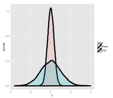
for $x=0,1, \ldots$. The mean of this distribution is $\lambda$. The variance of this distribution is also $\lambda$. Notice that $x$ ranges from 0 to $\infty$. Therefore, the Poisson distribution is especially useful for modeling unbounded counts.
统计代写|统计推断作业代写statistical inference代考|Limits of random variables
We’ll only talk about the limiting behavior of one statistic, the sample mean.
Fortunately, for the sample mean there’s a set of powerful results. These results allow us to talk about the large sample distribution of sample means of a collection of iid observations.
The first of these results we intuitively already know. It says that the average limits to what its estimating, the population mean. This result is called the Law of Large Numbers. It simply says that if you go to the trouble of collecting an infinite amount of data, you estimate the population mean perfectly. Note there’s sampling assumptions that have to hold for this result to be true. The data have to be iid.
A great example of this comes from coin flipping. Imagine if $\bar{X}_{n}$ is the average of the result of $n$ coin flips (i.e. the sample proportion of heads). The Law of Large Numbers states that as we flip a coin over and over, it eventually converges to the true probability of a head.
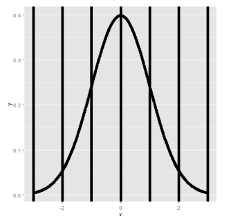
统计代写|统计推断作业代写statistical inference代考|The Central Limit Theorem
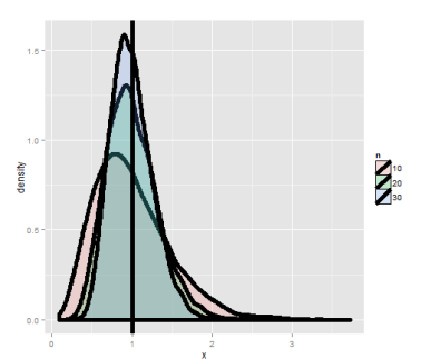
The Central Limit Theorem (CIT) is nne of the mnst important theorems in statistics. For our purposes, the CLT states that the distribution of averages of iid variables becomes that of a standard normal as the sample size increases.
Consider this fact for a second. We already know the mean and standard deviation of the distribution of averages from iid samples. The CLT gives us an approximation to the full distribution! Thus, for iid samples, we have a good sense of distribution of the average event though: (1) we only observed one average and (2) we don’t know what the population distribution is. Because of this, the CLT applies in an endless variety of settings and is one of the most important theorems ever discovered.
The formal result is that $\frac{\bar{X}{n}-\mu}{\sigma / \sqrt{n}}=\frac{\sqrt{n}\left(\bar{X}{n}-\mu\right)}{\sigma}=\frac{\text { Estimate }-\text { Mean of estimate }}{\text { Std. Err. of estimate }}$ has a distribution like that of a standard normal for large $n$. Replacing the standard error by its estimated value doesn’t change the CLT.
The useful way to think about the $\mathrm{CLT}$ is that $\bar{X}_{n}$ is approximately $N\left(\mu, \sigma^{2} / n\right)$.
统计推断代写
统计代写|统计推断作业代写statistical inference代考|The Poisson distribution
泊松分布用于对计数进行建模。它可能仅次于正态分布的有用性。事实上,伯努利分布、二项分布和多项分布都可以通过巧妙地使用泊松来建模。
泊松分布对于建模无限计数或每单位时间的计数(速率)特别有用。比如点击广告的次数,或者出现在公交车站的人数。(虽然这些原则上是有界的,但实际上很难为其设置上限。)泊松分布与所谓的流行模型之间也有很深的联系。
事件时间数据。此外,泊松分布是所谓列联表数据的默认模型,它只是离散特征的列表。最后,当n很大并且p很小,泊松是二项分布的精确近似。
泊松质量函数为:
磷(X=X;λ)=λX和−λX!
为了X=0,1,…. 这个分布的平均值是λ. 这个分布的方差也是λ. 请注意X范围从 0 到∞. 因此,泊松分布对于无界计数建模特别有用。
统计代写|统计推断作业代写statistical inference代考|Limits of random variables
我们只会讨论一个统计数据的限制行为,即样本均值。
幸运的是,对于样本均值,有一组强大的结果。这些结果使我们能够讨论 iid 观察集合的样本均值的大样本分布。
我们直观地已经知道这些结果中的第一个。它说平均限制了它的估计,人口的意思。这个结果被称为大数定律。它只是说,如果你不厌其烦地收集无限量的数据,你就可以完美地估计总体均值。请注意,必须保持抽样假设才能使此结果为真。数据必须是独立同分布的。
抛硬币就是一个很好的例子。想象一下,如果X¯n是结果的平均值n硬币翻转(即正面的样本比例)。大数定律指出,当我们一遍又一遍地掷硬币时,它最终会收敛到正面朝上的真实概率。
统计代写|统计推断作业代写statistical inference代考|The Central Limit Theorem
中心极限定理 (CIT) 是统计学中最重要的定理之一。出于我们的目的,CLT 指出,随着样本量的增加,独立同分布变量的平均值分布变为标准正态分布。
考虑一下这个事实。我们已经知道独立同分布样本的平均值分布的均值和标准差。CLT 为我们提供了完整分布的近似值!因此,对于 iid 样本,我们对平均事件的分布有很好的了解:(1)我们只观察到一个平均值,(2)我们不知道总体分布是什么。正因为如此,CLT 适用于无穷无尽的各种设置,并且是迄今为止发现的最重要的定理之一。
正式的结果是X¯n−μσ/n=n(X¯n−μ)σ= 估计 − 估计平均值 标准。呃。估计的 具有类似于大型标准正态分布的分布n. 用它的估计值替换标准误差不会改变 CLT。
思考问题的有用方法C大号吨就是它X¯n大约是ñ(μ,σ2/n).

统计代写请认准statistics-lab™. statistics-lab™为您的留学生涯保驾护航。统计代写|python代写代考
随机过程代考
在概率论概念中,随机过程是随机变量的集合。 若一随机系统的样本点是随机函数,则称此函数为样本函数,这一随机系统全部样本函数的集合是一个随机过程。 实际应用中,样本函数的一般定义在时间域或者空间域。 随机过程的实例如股票和汇率的波动、语音信号、视频信号、体温的变化,随机运动如布朗运动、随机徘徊等等。
贝叶斯方法代考
贝叶斯统计概念及数据分析表示使用概率陈述回答有关未知参数的研究问题以及统计范式。后验分布包括关于参数的先验分布,和基于观测数据提供关于参数的信息似然模型。根据选择的先验分布和似然模型,后验分布可以解析或近似,例如,马尔科夫链蒙特卡罗 (MCMC) 方法之一。贝叶斯统计概念及数据分析使用后验分布来形成模型参数的各种摘要,包括点估计,如后验平均值、中位数、百分位数和称为可信区间的区间估计。此外,所有关于模型参数的统计检验都可以表示为基于估计后验分布的概率报表。
广义线性模型代考
广义线性模型(GLM)归属统计学领域,是一种应用灵活的线性回归模型。该模型允许因变量的偏差分布有除了正态分布之外的其它分布。
statistics-lab作为专业的留学生服务机构,多年来已为美国、英国、加拿大、澳洲等留学热门地的学生提供专业的学术服务,包括但不限于Essay代写,Assignment代写,Dissertation代写,Report代写,小组作业代写,Proposal代写,Paper代写,Presentation代写,计算机作业代写,论文修改和润色,网课代做,exam代考等等。写作范围涵盖高中,本科,研究生等海外留学全阶段,辐射金融,经济学,会计学,审计学,管理学等全球99%专业科目。写作团队既有专业英语母语作者,也有海外名校硕博留学生,每位写作老师都拥有过硬的语言能力,专业的学科背景和学术写作经验。我们承诺100%原创,100%专业,100%准时,100%满意。
机器学习代写
随着AI的大潮到来,Machine Learning逐渐成为一个新的学习热点。同时与传统CS相比,Machine Learning在其他领域也有着广泛的应用,因此这门学科成为不仅折磨CS专业同学的“小恶魔”,也是折磨生物、化学、统计等其他学科留学生的“大魔王”。学习Machine learning的一大绊脚石在于使用语言众多,跨学科范围广,所以学习起来尤其困难。但是不管你在学习Machine Learning时遇到任何难题,StudyGate专业导师团队都能为你轻松解决。
多元统计分析代考
基础数据: $N$ 个样本, $P$ 个变量数的单样本,组成的横列的数据表
变量定性: 分类和顺序;变量定量:数值
数学公式的角度分为: 因变量与自变量
时间序列分析代写
随机过程,是依赖于参数的一组随机变量的全体,参数通常是时间。 随机变量是随机现象的数量表现,其时间序列是一组按照时间发生先后顺序进行排列的数据点序列。通常一组时间序列的时间间隔为一恒定值(如1秒,5分钟,12小时,7天,1年),因此时间序列可以作为离散时间数据进行分析处理。研究时间序列数据的意义在于现实中,往往需要研究某个事物其随时间发展变化的规律。这就需要通过研究该事物过去发展的历史记录,以得到其自身发展的规律。
回归分析代写
多元回归分析渐进(Multiple Regression Analysis Asymptotics)属于计量经济学领域,主要是一种数学上的统计分析方法,可以分析复杂情况下各影响因素的数学关系,在自然科学、社会和经济学等多个领域内应用广泛。
MATLAB代写
MATLAB 是一种用于技术计算的高性能语言。它将计算、可视化和编程集成在一个易于使用的环境中,其中问题和解决方案以熟悉的数学符号表示。典型用途包括:数学和计算算法开发建模、仿真和原型制作数据分析、探索和可视化科学和工程图形应用程序开发,包括图形用户界面构建MATLAB 是一个交互式系统,其基本数据元素是一个不需要维度的数组。这使您可以解决许多技术计算问题,尤其是那些具有矩阵和向量公式的问题,而只需用 C 或 Fortran 等标量非交互式语言编写程序所需的时间的一小部分。MATLAB 名称代表矩阵实验室。MATLAB 最初的编写目的是提供对由 LINPACK 和 EISPACK 项目开发的矩阵软件的轻松访问,这两个项目共同代表了矩阵计算软件的最新技术。MATLAB 经过多年的发展,得到了许多用户的投入。在大学环境中,它是数学、工程和科学入门和高级课程的标准教学工具。在工业领域,MATLAB 是高效研究、开发和分析的首选工具。MATLAB 具有一系列称为工具箱的特定于应用程序的解决方案。对于大多数 MATLAB 用户来说非常重要,工具箱允许您学习和应用专业技术。工具箱是 MATLAB 函数(M 文件)的综合集合,可扩展 MATLAB 环境以解决特定类别的问题。可用工具箱的领域包括信号处理、控制系统、神经网络、模糊逻辑、小波、仿真等。

![PDF] Theory-based Social Goal Inference | Semantic Scholar](data:image/svg+xml,%3Csvg%20xmlns='http://www.w3.org/2000/svg'%20viewBox='0%200%20516%20311'%3E%3C/svg%3E)