数学代写|凸优化作业代写Convex Optimization代考|Supremum and infimum
In mathematics, given a subset $S$ of a partially ordered set $T$, the supremum (sup) of $S$, if it exists, is the least element of $T$ that is greater than or equal to each element of $S$. Consequently, the supremum is also referred to as the least upper bound, lub or $L U B$. If the supremum exists, it may or may not belong to $S$. On the other hand, the infimum (inf) of $S$ is the greatest element in $T$, not necessarily in $S$, that is less than or equal to all elements of $S$. Consequently the
term greatest lower bound (also abbreviated as glb or GLB) is also commonly used. Consider a set $C \subseteq \mathbb{R}$.
A number $a$ is an upper bound (lower bound) on $C$ if for each $x \in C, x \leq$ $a(x \geq a)$.
A number $b$ is the least upper bound (greatest lower bound) or the supremum (infimum) of $C$ if (i) $b$ is an upper bound (lower bound) on $C$, and (ii) $b \leq a(b \geq a)$ for every upper bound (lower bound) $a$ on $C$. Remark $1.8$ An infimum is in a precise sense dual to the concept of a supremum and vice versa. For instance, sup $C=\infty$ if $C$ is unbounded above and inf $C=$ $-\infty$ if $C$ is unbounded below.
数学代写|凸优化作业代写Convex Optimization代考|Derivative and gradient
Since vector limits are computed by taking the limit of each coordinate function, we can write the function $f: \mathbb{R}^{n} \rightarrow \mathbb{R}^{m}$ for a point $\mathbf{x} \in \mathbb{R}^{n}$ as follows: $$ \boldsymbol{f}(\mathbf{x})=\left[\begin{array}{c} f_{1}(\mathbf{x}) \ f_{2}(\mathbf{x}) \ \vdots \ f_{m}(\mathbf{x}) \end{array}\right]=\left(f_{1}(\mathbf{x}), f_{2}(\mathbf{x}), \ldots, f_{m}(\mathbf{x})\right) $$ where each $f_{i}(\mathbf{x})$ is a function from $\mathbb{R}^{n}$ to $\mathbb{R}$. Now, $\frac{\partial \boldsymbol{f}(\mathbf{x})}{\partial x_{j}}$ can be defined as $$ \frac{\partial \boldsymbol{f}(\mathbf{x})}{\partial x_{j}}=\left[\begin{array}{c} \frac{\partial f_{1}(\mathbf{x})}{\partial x_{j}} \ \frac{\partial f_{2}(\mathbf{x})}{\partial x_{j}} \ \vdots \ \frac{\partial f_{m}(\mathbf{x})}{\partial x_{j}} \end{array}\right]=\left(\frac{\partial f_{1}(\mathbf{x})}{\partial x_{j}}, \frac{\partial f_{2}(\mathbf{x})}{\partial x_{j}}, \ldots, \frac{\partial f_{m}(\mathbf{x})}{\partial x_{j}}\right) $$ The above vector is a tangent vector at the point $\mathbf{x}$ of the curve $\boldsymbol{f}$ obtained by varying only $x_{j}$ (the $j$ th coordinate of $\mathbf{x}$ ) with $x_{i}$ fixed for all $i \neq j$.
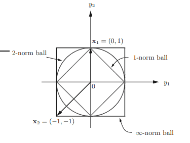
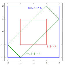
The norm ball of a point $\mathbf{x} \in \mathbb{R}^{n}$ is defined as the following set ${ }^{1}$ $$ B(\mathbf{x}, r)=\left{\mathbf{y} \in \mathbb{R}^{n} \mid|\mathbf{y}-\mathbf{x}| \leq r\right} . $$ where $r$ is the radius and $\mathbf{x}$ is the center of the norm ball. It is also called the neighborhood of the point $\mathbf{x}$. For the case of $n=2, \mathbf{x}=\mathbf{0}{2}$, and $r=1$, the 2 norm ball is $B(\mathbf{x}, r)=\left{\mathbf{y} \mid y{1}^{2}+y_{2}^{2} \leq 1\right}$ (a circular disk of radius equal to 1 ), the 1-norm ball is $B(\mathbf{x}, r)=\left{\mathbf{y}|| y_{1}|+| y_{2} \mid \leq 1\right}$ (a 2-dimensional cross-polytope of area equal to 2 ), and the $\infty$-norm ball is $B(\mathbf{x}, r)=\left{\mathbf{y}|| y_{1}|\leq 1,| y_{2} \mid \leq 1\right$,$} (a$ square of area equal to 4) (see Figure 1.1). Note that the norm ball is symmetric with respect to (w.r.t.) the origin, convex, closed, bounded and has nonempty interior. Moreover, the 1-norm ball is a subset of the 2-norm ball which is a subset of $\infty$-norm ball, due to the following inequality: $$ |\mathbf{v}|_{p} \leq|\mathbf{v}|_{q} $$ where $\mathbf{v} \in \mathbb{R}^{n}, p$ and $q$ are real and $p>q \geq 1$, and the equality holds when $\mathbf{v}=$ re $_{i}$, i.e., all the $p$-norm balls of constant radius $r$ have intersections at $r \mathbf{e}{i}, i=$ $1, \ldots, n$. For instance, in Figure 1.1, $\left|\mathbf{x}{1}\right|_{p}=1$ for all $p \geq 1$, and $\left|\mathbf{x}{2}\right|{\infty}=1<$ $\left|\mathbf{x}{2}\right|{2}=\sqrt{2}<\left|\mathbf{x}{2}\right|{1}=2$. The inequality (1.17) is proven as follows.
数学代写|凸优化作业代写Convex Optimization代考|Interior point
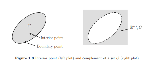
A point $\mathbf{x}$ in a set $C \subseteq \mathbb{R}^{n}$ is an interior point of the set $C$ if there exists an $\epsilon>0$ for which $B(\mathbf{x}, \epsilon) \subseteq C$ (see Figure 1.3). In other words, a point $\mathbf{x} \in C$ is said to be an interior point of the set $C$ if the set $C$ contains some neighborhood of $\mathbf{x}$, that is, if all points within some neighborhood of $\mathbf{x}$ are also in $C$.
Remark $1.7$ The set of all the interior points of $C$ is called the interior of $C$ and is represented as int $C$, which can also be expressed as $$ \text { int } C={\mathbf{x} \in C \mid B(\mathbf{x}, r) \subseteq C \text {, for some } r>0} \text {, } $$ which will be frequently used in many proofs directly or indirectly in the ensuing chapters. Complement, scaled sets, and sum of sets The complement of a set $C \subset \mathbb{R}^{n}$ is defined as follows (see Figure 1.3): $$ \mathbb{R}^{n} \backslash C=\left{\mathbf{x} \in \mathbb{R}^{n} \mid \mathbf{x} \notin C\right}, $$ where ” $\backslash$ ” denotes the set difference, i.e., $A \backslash B={\mathbf{x} \in A \mid \mathbf{x} \notin B}$. The set $C \subset$ $\mathbb{R}^{n}$ scaled by a real number $\alpha$ is a set defined as $$ \alpha \cdot C \triangleq{\alpha \mathbf{x} \mid \mathbf{x} \in C} $$
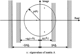
In mathematics, a matrix norm is a natural extension of the notion of a vector norm to matrices. Some useful matrix norms needed throughout the book are introduced next. The Frobenius norm of an $m \times n$ matrix $\mathbf{A}$ is defined as $$ |\mathbf{A}|_{\mathrm{F}}=\left(\sum_{i=1}^{m} \sum_{j=1}^{n}\left|[\mathbf{A}]{i j}\right|^{2}\right)^{1 / 2}=\sqrt{\operatorname{Tr}\left(\mathbf{A}^{T} \mathbf{A}\right)} $$ where $$ \operatorname{Tr}(\mathbf{X})=\sum{i=1}^{n}[\mathbf{X}]_{i i} $$ denotes the trace of a square matrix $\mathbf{X} \in \mathbb{R}^{n \times n}$. As $n=1$, A reduces to a column vector of dimension $m$ and its Frobenius norm also reduces to the 2 -norm of the vector.
The other class of norm is known as the induced norm or operator norm. Suppose that $|\cdot|_{a}$ and $|\cdot|_{b}$ are norms on $\mathbb{R}^{m}$ and $\mathbb{R}^{n}$, respectively. Then the operator/induced norm of $\mathbf{A} \in \mathbb{R}^{m \times n}$, induced by the norms $|\cdot|_{a}$ and $\left|_{\cdot}\right|_{b}$, is defined as $$ |\mathbf{A}|_{a, b}=\sup \left{|\mathbf{A} \mathbf{u}|_{a} \mid|\mathbf{u}|_{b} \leq 1\right} $$ where $\sup (C)$ denotes the least upper bound of the set $C$. As $a=b$, we simply denote $|\mathbf{A}|_{a, b}$ by $|\mathbf{A}|_{a}$. Commonly used induced norms of an $m \times n$ matrix $$ \mathbf{A}=\left{a_{i j}\right}_{m \times n}=\left[\mathbf{a}{1}, \ldots, \mathbf{a}{n}\right] $$ are as follows: $$ \begin{aligned} |\mathbf{A}|_{1} &=\max {|\mathbf{u}|{1} \leq 1} \sum_{j=1}^{n} u_{j} \mathbf{a}{j} |{1}, \quad(a=b=1) \ & \leq \max {|\mathbf{u}|{1} \leq 1} \sum_{j=1}^{n}\left|u_{j}\right| \cdot\left|\mathbf{a}{j}\right|{1} \text { (by triangle inequality) } \ &=\max {1 \leq j \leq n}\left|\mathbf{a}{j}\right|_{1}=\max {1 \leq j \leq n} \sum{i=1}^{m}\left|a_{i j}\right| \end{aligned} $$
数学代写|凸优化作业代写Convex Optimization代考|Inner product
The inner product of two real vectors $\mathbf{x} \in \mathbb{R}^{n}$ and $\mathbf{y} \in \mathbb{R}^{n}$ is a real scalar and is defined as $$ \langle\mathbf{x}, \mathbf{y}\rangle=\mathbf{y}^{T} \mathbf{x}=\sum_{i=1}^{n} x_{i} y_{i} $$ If $\mathbf{x}$ and $\mathbf{y}$ are complex vectors, then the transpose in the above equation will be replaced by Hermitian. Note that the square root of the inner product of a vector $\mathbf{x}$ with itself gives the Euclidean norm of that vector.
Cauchy-Schwartz inequality: For any two vectors $\mathbf{x}$ and $\mathbf{y}$ in $\mathbb{R}^{n}$, the CauchySchwartz inequality $$ |\langle\mathbf{x}, \mathbf{y}\rangle| \leq|\mathbf{x}|_{2} \cdot|\mathbf{y}|_{2} $$ holds. Furthermore, the equality holds if and only if $\mathbf{x}=\alpha \mathbf{y}$ for some $\alpha \in \mathbb{R}$. Pythagorean theorem: If two vectors $\mathbf{x}$ and $\mathbf{y}$ in $\mathbb{R}^{n}$ are orthogonal, i.e., $\langle\mathbf{x}, \mathbf{y}\rangle=0$, then $$ |\mathbf{x}+\mathbf{y}|_{2}^{2}=(\mathbf{x}+\mathbf{y})^{T}(\mathbf{x}+\mathbf{y})=|\mathbf{x}|_{2}^{2}+2(\mathbf{x}, \mathbf{y}\rangle+|\mathbf{y}|_{2}^{2}=|\mathbf{x}|_{2}^{2}+|\mathbf{y}|_{2}^{2} $$
数学代写|凸优化作业代写Convex Optimization代考|Definition and examples
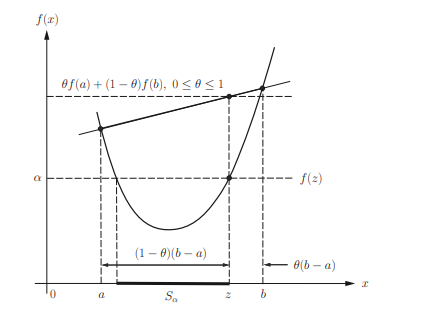
A function $f: \mathbb{R}^{n} \rightarrow \mathbb{R}$ is said to be quasiconvex if its domain and all its $\alpha$ sublevel sets defined as $$ S_{a}={\mathbf{x} \mid \mathbf{x} \in \operatorname{dom} f, f(\mathbf{x}) \leq \alpha} $$ (see Figure $3.8$ ) are convex for every $\alpha$. Moreover,
$f$ is quasiconvex if $f$ is convex since every sublevel set of convex functions is a convex set (cf. Remark 3.5), but the converse is not necessarily true.
$f$ is quasiconcave if $-f$ is quasiconvex. It is also true that $f$ is quasiconcave if its domain and all the $\alpha$-superlevel sets defined as
A function $f: \mathbb{R}^{n} \rightarrow \mathbb{R}$ is quasiconvex if and only if $$ f(\theta \mathbf{x}+(1-\theta) \mathbf{y}) \leq \max {f(\mathbf{x}), f(\mathbf{y})} $$ for all $\mathbf{x}, \mathbf{y} \in \operatorname{dom} f$, and $0 \leq \theta \leq 1$ (see Figure $3.8$ ). Proof: Let us prove the necessity followed by sufficiency.
Necessity: Let $\mathbf{x}, \mathbf{y} \in \operatorname{dom} f$. Choose $\alpha=\max {f(\mathbf{x}), f(\mathbf{y})}$. Then $\mathbf{x}, \mathbf{y} \in S_{\alpha}$. Since $f$ is quasiconvex by assumption, $S_{\alpha}$ is convex, that is, for $\theta \in[0,1]$, $$ \begin{aligned} &\theta \mathbf{x}+(1-\theta) \mathbf{y} \in S_{\alpha} \ &\Rightarrow f(\theta \mathbf{x}+(1-\theta) \mathbf{y}) \leq \alpha=\max {f(\mathbf{x}), f(\mathbf{y})} \end{aligned} $$
Sufficiency: For every $\alpha$, pick two points $\mathbf{x}, \mathbf{y} \in S_{\alpha} \Rightarrow f(\mathbf{x}) \leq \alpha, f(\mathbf{y}) \leq \alpha$. Since for $0 \leq \theta \leq 1, f(\theta \mathbf{x}+(1-\theta) \mathbf{y}) \leq \max {f(\mathbf{x}), f(\mathbf{y})} \leq \alpha($ by $(3.106))$, we have $$ \theta \mathbf{x}+(1-\theta) \mathbf{y} \in S_{\alpha} $$ Therefore, $S_{\alpha}$ is convex and thus the function $f$ is quasiconvex. Remark 3.33 $f$ is quasiconcave if and only if $$ f(\theta \mathbf{x}+(1-\theta) \mathbf{y}) \geq \min {f(\mathbf{x}), f(\mathbf{y})} $$ for all $\mathbf{x}, \mathbf{y} \in \operatorname{dom} f$, and $0 \leq \theta \leq 1$. This is also the modified Jensen’s inequality for quasiconcave functions. If the inequality (3.106) holds strictly for $0<\theta<1$, then $f$ is strictly quasiconvex. Similarly, if the inequality (3.107) holds strictly for $0<\theta<1$, then $f$ is strictly quasiconcave. Remark 3.34 Since the rank of a PSD matrix is quasiconcave, $$ \operatorname{rank}(\mathbf{X}+\mathbf{Y}) \geq \min {\operatorname{rank}(\mathbf{X}), \operatorname{rank}(\mathbf{Y})}, \mathbf{X}, \mathbf{Y} \in \mathbb{S}{+}^{\mathrm{n}} $$ holds true. This can be proved by (3.107), by which we get $$ \operatorname{rank}(\theta \mathbf{X}+(1-\theta) \mathbf{Y}) \geq \min {\operatorname{rank}(\mathbf{X}), \operatorname{rank}(\mathbf{Y})} $$ for all $\mathbf{X} \in \mathbb{S}{+}^{n}, \mathbf{Y} \in \mathbb{S}_{+}^{n}$, and $0 \leq \theta \leq 1$. Then replacing $\mathbf{X}$ by $\mathbf{X} / \theta$ and $\mathbf{Y}$ by $\mathbf{Y} /(1-\theta)$ where $\theta \neq 0$ and $\theta \neq 1$ gives rise to (3.108).
Remark $3.35 \operatorname{card}(\mathbf{x}+\mathbf{y}) \geq \min {\operatorname{card}(\mathbf{x}), \operatorname{card}(\mathbf{y})}, \mathbf{x}, \mathbf{y} \in \mathbb{R}_{+}^{n}$. Similar to the proof of (3.108) in Remark $3.34$, this inequality can be shown to be true by using $(3.107)$ again, since $\operatorname{card}(\mathrm{x})$ is quasiconcave.
Suppose that $f$ is differentiable. Then $f$ is quasiconvex if and only if dom $f$ is convex and for all $\mathbf{x}, \mathbf{y} \in \operatorname{dom} f$ $$ f(\mathbf{y}) \leq f(\mathbf{x}) \Rightarrow \nabla f(\mathbf{x})^{T}(\mathbf{y}-\mathbf{x}) \leq 0, $$ that is, $\nabla f(\mathbf{x})$ defines a supporting hyperplane to the sublevel set $$ S_{\alpha=f(\mathbf{x})}={\mathbf{y} \mid f(\mathbf{y}) \leq \alpha=f(\mathbf{x})} $$ at the point $\mathbf{x}$ (see Figure 3.11). Moreover, the first-order condition given by (3.110) means that the first-order term in the Taylor series of $f(\mathbf{y})$ at the point $\mathbf{x}$ is no greater than zero whenever $f(\mathbf{y}) \leq f(\mathbf{x})$. Proof: Let us prove the necessity followed by the sufficiency.
Necessity: Suppose $f(\mathbf{x}) \geq f(\mathbf{y})$. Then, by modified Jensen’s inequality, we have $$ f(t \mathbf{y}+(1-t) \mathbf{x}) \leq f(\mathbf{x}) \text { for all } 0 \leq t \leq 1 $$ Therefore, $$ \begin{aligned} \lim {t \rightarrow 0^{+}} \frac{f(\mathbf{x}+t(\mathbf{y}-\mathbf{x}))-f(\mathbf{x})}{t} &=\lim {t \rightarrow 0^{+}} \frac{1}{t}\left(f(\mathbf{x})+t \nabla f(\mathbf{x})^{T}(\mathbf{y}-\mathbf{x})-f(\mathbf{x})\right) \ &=\nabla f(\mathbf{x})^{T}(\mathbf{y}-\mathbf{x}) \leq 0 \end{aligned} $$ where we have used the first-order Taylor series approximation in the first equality.
Sufficiency: Suppose that $f(\mathbf{x})$ is not quasiconvex. Then there exists a nonconvex sublevel set of $f$, $$ S_{\alpha}={\mathbf{x} \mid f(\mathbf{x}) \leq \alpha}, $$ and two distinct points $\mathbf{x}{1}, \mathbf{x}{2} \in S_{\alpha}$ such that $\theta \mathbf{x}{1}+(1-\theta) \mathbf{x}{2} \notin$ $S_{\alpha}$, for some $0<\theta<1$, i.e., $$ f\left(\theta \mathbf{x}{1}+(1-\theta) \mathbf{x}{2}\right)>\alpha \text { for some } 0<\theta<1 . $$ Since $f$ is differentiable, hence continuous, (3.112) implies that, as illustrated in Figure 3.12, there exist distinct $\theta_{1}, \theta_{2} \in(0,1)$ such that $$ \begin{aligned} &f\left(\theta \mathbf{x}_{1}+(1-\theta) \mathbf{x}_{2}\right)>\alpha \text { for all } \theta_{1}<\theta<\theta_{2} \ &f\left(\theta_{1} \mathbf{x}{1}+\left(1-\theta{1}\right) \mathbf{x}{2}\right)=f\left(\theta{2} \mathbf{x}{1}+\left(1-\theta{2}\right) \mathbf{x}{2}\right)=\alpha . \end{aligned} $$ Let $\mathbf{x}=\theta{1} \mathbf{x}{1}+\left(1-\theta{1}\right) \mathbf{x}{2}$ and $\mathbf{y}=\theta{2} \mathbf{x}{1}+\left(1-\theta{2}\right) \mathbf{x}_{2}$, and so $$ f(\mathbf{x})=f(\mathbf{y})=\alpha, $$ and $$ g(t)=f(t \mathbf{y}+(1-t) \mathbf{x})>\alpha \text { for all } 0<t<1 $$
is a differentiable function of $t$ and $\partial g(t) / \partial t>0$ for $t \in[0, \varepsilon)$ where $0<\varepsilon \ll 1$, as illustrated in Figure 3.12. Then, it can be inferred that $$ \begin{aligned} (1-t) \frac{\partial g(t)}{\partial t} &=\nabla f(\mathbf{x}+t(\mathbf{y}-\mathbf{x}))^{T}[(1-t)(\mathbf{y}-\mathbf{x})]>0 \text { for all } t \in[0, \varepsilon) \ &=\nabla f(\boldsymbol{x})^{T}(\mathbf{y}-\boldsymbol{x})>0 \text { for all } t \in[0, \varepsilon) \end{aligned} $$ where $$ \begin{aligned} \boldsymbol{x} &=\mathbf{x}+t(\mathbf{y}-\mathbf{x}), \quad t \in[0, \varepsilon] \ \Rightarrow g(t) &=f(\boldsymbol{x}) \geq f(\mathbf{y})=\alpha(\text { by }(3.113) \text { and }(3.114)) \end{aligned} $$ Therefore, if $f$ is not quasiconvex, there exist $\boldsymbol{x}, \mathbf{y}$ such that $f(\mathbf{y}) \leq f(\boldsymbol{x})$ and $\nabla f(\boldsymbol{x})^{T}(\mathbf{y}-\boldsymbol{x})>0$, which contradicts with the implication (3.110). Thus we have completed the proof of sufficiency.
数学代写|凸优化作业代写Convex Optimization代考|Nonnegative weighted sum
Let $f_{1}, \ldots, f_{m}$ be convex functions and $w_{1}, \ldots, w_{m} \geq 0$. Then $\sum_{i=1}^{m} w_{i} f_{i}$ is convex.
Proof: $\operatorname{dom}\left(\sum_{i=1}^{m} w_{i} f_{i}\right)=\bigcap_{i=1}^{m}$ dom $f_{i}$ is convex because dom $f_{i}$ is convex for all $i$. For $0 \leq \theta \leq 1$, and $\mathbf{x}, \mathbf{y} \in \operatorname{dom}\left(\sum_{i=1}^{m} w_{i} f_{i}\right)$, we have $$ \begin{aligned} \sum_{i=1}^{m} w_{i} f_{i}(\theta \mathbf{x}+(1-\theta) \mathbf{y}) & \leq \sum_{i=1}^{m} w_{i}\left(\theta f_{i}(\mathbf{x})+(1-\theta) f_{i}(\mathbf{y})\right) \ &=\theta \sum_{i=1}^{m} w_{i} f_{i}(\mathbf{x})+(1-\theta) \sum_{i=1}^{m} w_{i} f_{i}(\mathbf{y}) \end{aligned} $$ Hence proved. Remark 3.27 $f(\mathbf{x}, \mathbf{y})$ is convex in $\mathbf{x}$ for each $\mathbf{y} \in \mathcal{A}$ and $w(\mathbf{y}) \geq 0$. Then, $$ g(\mathbf{x})=\int_{\mathcal{A}} w(\mathbf{y}) f(\mathbf{x}, \mathbf{y}) d \mathbf{y} $$ is convex on $\bigcap_{y \in \mathcal{A}} \operatorname{dom} f$. Composition with affine mapping If $f: \mathbb{R}^{n} \rightarrow \mathbb{R}$ is a convex function, then for $\mathbf{A} \in \mathbb{R}^{n \times m}$ and $\mathbf{b} \in \mathbb{R}^{n}$, the function $g: \mathbb{R}^{m} \rightarrow \mathbb{R}$, defined as $$ g(\mathbf{x})=f(\mathbf{A} \mathbf{x}+\mathbf{b}), $$ is also convex and its domain can be expressed as $$ \begin{aligned} \operatorname{dom} g &=\left{\mathbf{x} \in \mathbb{R}^{m} \mid \mathbf{A} \mathbf{x}+\mathbf{b} \in \operatorname{dom} f\right} \ &=\left{\mathbf{A}^{\dagger}(\mathbf{y}-\mathbf{b}) \mid \mathbf{y} \in \mathbf{d o m} f\right}+\mathcal{N}(\mathbf{A}) \quad(\text { cf. }(2.62)) \end{aligned} $$ which is also a convex set by Remark $2.9$. Proof (using epigraph): Since $g(\mathbf{x})=f(\mathbf{A x}+\mathbf{b})$ and epi $f={(\mathbf{y}, t) \mid f(\mathbf{y}) \leq t}$, we have $$ \text { epi } \begin{aligned} g &=\left{(\mathbf{x}, t) \in \mathbb{R}^{m+1} \mid f(\mathbf{A} \mathbf{x}+\mathbf{b}) \leq t\right} \ &=\left{(\mathbf{x}, t) \in \mathbb{R}^{m+1} \mid(\mathbf{A} \mathbf{x}+\mathbf{b}, t) \in \mathbf{e p i} f\right} \end{aligned} $$
Now, define $$ \mathcal{S}=\left{(\mathbf{x}, \mathbf{y}, t) \in \mathbb{R}^{m+n+1} \mid \mathbf{y}=\mathbf{A} \mathbf{x}+\mathbf{b}, f(\mathbf{y}) \leq t\right} $$ so that $$ \text { epi } g=\left{\left[\begin{array}{lll} \mathbf{I}{m} & \mathbf{0}{m \times n} & \mathbf{0}{m} \ \mathbf{0}{m}^{T} & \mathbf{0}{\mathrm{n}}^{T} & 1 \end{array}\right](\mathbf{x}, \mathbf{y}, t) \mid(\mathbf{x}, \mathbf{y}, t) \in \mathcal{S}\right} $$ which is nothing but the image of $\mathcal{S}$ via an affine mapping. It can be easily shown, by the definition of convex sets, that $\mathcal{S}$ is convex if $f$ is convex. Therefore epi $g$ is convex (due to affine mapping from the convex set $\mathcal{S}$ ) implying that $g$ is convex (by Fact 3.2). Alternative proof: For $0 \leq \theta \leq 1$, we have $$ \begin{aligned} g\left(\theta \mathbf{x}{1}+(1-\theta) \mathbf{x}{2}\right) &=f\left(\mathbf{A}\left(\theta \mathbf{x}{1}+(1-\theta) \mathbf{x}{2}\right)+\mathbf{b}\right) \ &=f\left(\theta\left(\mathbf{A} \mathbf{x}{1}+\mathbf{b}\right)+(1-\theta)\left(\mathbf{A} \mathbf{x}{2}+\mathbf{b}\right)\right) \ & \leq \theta f\left(\mathbf{A} \mathbf{x}{1}+\mathbf{b}\right)+(1-\theta) f\left(\mathbf{A} \mathbf{x}{2}+\mathbf{b}\right) \ &=\theta g\left(\mathbf{x}{1}\right)+(1-\theta) g\left(\mathbf{x}_{2}\right) \end{aligned} $$ Moreover, dom $g$ (cf. (3.72)) is also a convex set, and so we conclude that $f(\mathbf{A} \mathbf{x}+\mathbf{b})$ is a convex function.
Suppose that $h: \operatorname{dom} h \rightarrow \mathbb{R}$ is a convex (concave) function and dom $h \subset \mathbb{R}^{n}$. The extended-value extension of $h$, denoted as $\tilde{h}$, with $\operatorname{dom} \tilde{h}=\mathbb{R}^{n}$ aids in simple representation as its domain is the entire $\mathbb{R}^{n}$, which need not be explicitly mentioned. The extended-valued function $\tilde{h}$ is a function taking the same value of $h(\mathbf{x})$ for $\mathbf{x} \in$ dom $h$, otherwise taking the value of $+\infty(-\infty)$. Specifically, if $h$ is convex, $$ \tilde{h}(\mathbf{x})=\left{\begin{array}{l} h(\mathbf{x}), \mathbf{x} \in \operatorname{dom} h \ +\infty, \mathbf{x} \notin \operatorname{dom} h \end{array}\right. $$ and if $h$ is concave, $$ \tilde{h}(\mathbf{x})=\left{\begin{array}{l} h(\mathbf{x}), \mathbf{x} \in \operatorname{dom} h \ -\infty, \mathbf{x} \notin \operatorname{dom} h \end{array}\right. $$ Then the extended-valued function $\tilde{h}$ does not affect the convexity (or concavity) of the original function $h$ and Eff-dom $\tilde{h}=$ Eff-dom $h$.
Some examples for illustrating properties of an extended-value extension of a function are as follows.
$h(x)=\log x$, $\operatorname{dom} h=\mathbb{R}_{++}$. Then $h(x)$ is concave and $\tilde{h}(x)$ is concave and nondecreasing.
$h(x)=x^{1 / 2}$, dom $h=\mathbb{R}_{+}$. Then $h(x)$ is concave and $\tilde{h}(x)$ is concave and nondecreasing.
In the function $$ h(x)=x^{2}, x \geq 0, $$ i.e., dom $h=\mathbb{R}_{+}, h(x)$ is convex and $\tilde{h}(x)$ is convex but neither nondecreasing nor nonincreasing.
Let $f(\mathbf{x})=h(g(\mathbf{x}))$, where $h: \mathbb{R} \rightarrow \mathbb{R}$ and $g: \mathbb{R}^{n} \rightarrow \mathbb{R}$. Then we have the following four composition rules about the convexity or concavity of $f$. (a) $f$ is convex if $h$ is convex, $\bar{h}$ nondecreasing, and $g$ convex. (3.76a) (b) $f$ is convex if $h$ is convex, $\tilde{h}$ nonincreasing, and $g$ concave. (3.76b) (c) $f$ is concave if $h$ is concave, $\tilde{h}$ nondecreasing, and $g$ concave. (3.76c) (d) $f$ is concave if $h$ is concave, $\tilde{h}$ nonincreasing, and $g$ convex. (3.76d) Consider the case that $g$ and $h$ are twice differentiable and $\tilde{h}(x)=h(x)$. Then, $$ \nabla f(\mathbf{x})=h^{\prime}(g(\mathbf{x})) \nabla g(\mathbf{x}) $$ and $$ \begin{aligned} \nabla^{2} f(\mathbf{x}) &=D(\nabla f(\mathbf{x}))=D\left(h^{\prime}(g(\mathbf{x})) \cdot \nabla g(\mathbf{x})\right) \quad(\text { by }(1.46)) \ &=\nabla g(\mathbf{x}) D\left(h^{\prime}(g(\mathbf{x}))\right)+h^{\prime}(g(\mathbf{x})) \cdot D(\nabla g(\mathbf{x})) \ &=h^{\prime \prime}(g(\mathbf{x})) \nabla g(\mathbf{x}) \nabla g(\mathbf{x})^{T}+h^{\prime}(g(\mathbf{x})) \nabla^{2} g(\mathbf{x}) \end{aligned} $$ The composition rules (a) (cf. (3.76a)) and (b) (cf. (3.76b)) can be proven for convexity of $f$ by checking if $\nabla^{2} f(\mathbf{x}) \succeq \mathbf{0}$, and the composition rules (c) (cf. $(3.76 \mathrm{c}))$ and (d) (cf. $(3.76 \mathrm{~d}))$ for concavity of $f$ by checking if $\nabla^{2} f(\mathbf{x}) \preceq \mathbf{0}$. Let us conclude this subsection with a simple example. Example $3.3$ Let $g(\mathbf{x})=|\mathbf{x}|_{2}$ (convex) and $$ h(x)= \begin{cases}x^{2}, & x \geq 0 \ 0, & \text { otherwise }\end{cases} $$ which is convex. So $\tilde{h}(x)=h(x)$ is nondecreasing. Then, $f(\mathbf{x})=h(g(\mathbf{x}))=$ $|\mathbf{x}|_{2}^{2}=\mathbf{x}^{T} \mathbf{x}$ is convex by $(3.76 \mathrm{a})$, or by the second-order condition $\nabla^{2} f(\mathbf{x})=$ $2 \mathbf{I}_{n} \succ \mathbf{0}, f$ is indeed convex.
数学代写|凸优化作业代写Convex Optimization代考|Pointwise minimum and infimum
If $f(\mathbf{x}, \mathbf{y})$ is convex in $(\mathbf{x}, \mathbf{y}) \in \mathbb{R}^{m} \times \mathbb{R}^{n}$ and $C \subset \mathbb{R}^{n}$ is convex and nonempty, then $$ g(\mathbf{x})=\inf {\mathbf{y} \in C} f(\mathbf{x}, \mathbf{y}) $$ is convex, provided that $g(\mathbf{x})>-\infty$ for some $\mathbf{x}$. Similarly, if $f(\mathbf{x}, \mathbf{y})$ is concave in $(\mathbf{x}, \mathbf{y}) \in \mathbb{R}^{m} \times \mathbb{R}^{n}$, then $$ \tilde{g}(\mathbf{x})=\sup {\mathbf{y} \in C} f(\mathbf{x}, \mathbf{y}) $$ is concave provided that $C \subset \mathbb{R}^{n}$ is convex and nonempty and $\tilde{g}(\mathbf{x})<\infty$ for some $\mathbf{x}$. Next, we present the proof for the former.
Proof of (3.87): Since $f$ is continuous over int(dom $f$ ) (cf. Remark 3.7), for any $\epsilon>0$ and $\mathbf{x}{1}, \mathbf{x}{2} \in \operatorname{dom} g$, there exist $\mathbf{y}{1}, \mathbf{y}{2} \in C$ (depending on $\epsilon$ ) such that $$ f\left(\mathbf{x}{i}, \mathbf{y}{i}\right) \leq g\left(\mathbf{x}{i}\right)+\epsilon, i=1,2 . $$ Let $\left(\mathbf{x}{1}, t_{1}\right),\left(\mathbf{x}{2}, t{2}\right) \in$ epi $g$. Then $g\left(\mathbf{x}{i}\right)=\inf {\mathbf{y} \in C} f\left(\mathbf{x}{i}, \mathbf{y}\right) \leq t{i}, i=1,2$. Then for any $\theta \in[0,1]$, we have $$ \begin{aligned} g\left(\theta \mathbf{x}{1}+(1-\theta) \mathbf{x}{2}\right) &=\inf {\mathbf{y} \in C} f\left(\theta \mathbf{x}{1}+(1-\theta) \mathbf{x}{2}, \mathbf{y}\right) \ & \leq f\left(\theta \mathbf{x}{1}+(1-\theta) \mathbf{x}{2}, \theta \mathbf{y}{1}+(1-\theta) \mathbf{y}{2}\right) \ & \leq \theta f\left(\mathbf{x}{1}, \mathbf{y}{1}\right)+(1-\theta) f\left(\mathbf{x}{2}, \mathbf{y}{2}\right) \quad \text { (since } f \text { is convex) } \ & \leq \theta g\left(\mathbf{x}{1}\right)+(1-\theta) g\left(\mathbf{x}{2}\right)+\epsilon \quad \text { (by (3.89)) } \ & \leq \theta t{1}+(1-\theta) t_{2}+\epsilon . \end{aligned} $$ It can be seen that as $\epsilon \rightarrow 0, g\left(\theta \mathbf{x}{1}+(1-\theta) \mathbf{x}{2}\right) \leq \theta t_{1}+(1-\theta) t_{2}$, implying $\left(\theta \mathbf{x}{1}+(1-\theta) \mathbf{x}{2}, \theta t_{1}+(1-\theta) t_{2}\right) \in$ epi $g$. Hence epi $g$ is a convex set, and thus $g(\mathbf{x})$ is a convex function by Fact 3.2.
Alternative proof of (3.87): Because dom $g={\mathbf{x} \mid(\mathbf{x}, \mathbf{y}) \in \operatorname{dom} f, \mathbf{y} \in C}$ is the projection of the convex set ${(\mathbf{x}, \mathbf{y}) \mid(\mathbf{x}, \mathbf{y}) \in \operatorname{dom} f, \mathbf{y} \in C}$ on the $\mathbf{x}-$ coordinate, it must be a convex set (cf. Remark 2.11).
数学代写|凸优化作业代写Convex Optimization代考|Basic properties and examples of convex functions
Prior to introducing the definition, properties and various conditions of convex functions together with illustrative examples, we need to clarify the role of $+\infty$ and $-\infty$ for a function $f: \mathbb{R}^{n} \rightarrow \mathbb{R}$. In spite of $+\infty,-\infty \notin \mathbb{R}, f(\mathbf{x})$ is allowed to take a value of $+\infty$ or $-\infty$ for some $\mathrm{x} \in \operatorname{dom} f$, hereafter. For instance, the following functions $f_{1}(\mathbf{x})=\left{\begin{array}{l}|\mathbf{x}|_{2}^{2},|\mathbf{x}|_{2} \leq 1 \ +\infty, \quad 1<|\mathbf{x}|_{2} \leq 2\end{array}, \quad\right.$ dom $f_{1}=\left{\mathbf{x} \in \mathbb{R}^{n} \mid|\mathbf{x}|_{2} \leq 2\right}$ $f_{2}(x)=\left{\begin{array}{l}-\infty, x=0 \ \log x, x>0\end{array}, \quad \operatorname{dom} f_{2}=\mathbb{R}{+}\right.$ are well-defined functions, and $f{1}$ is a convex function and $f_{2}$ is a concave function. The convexity of functions will be presented next in detail. Definition and fundamental properties A function $f: \mathbb{R}^{n} \rightarrow \mathbb{R}$ is said to be convex if the following conditions are satisfied
dom $f$ is convex.
For all $\mathbf{x}, \mathbf{y} \in \operatorname{dom} f, \theta \in[0,1]$. $$ f(\theta \mathbf{x}+(1-\theta) \mathbf{y}) \leq \theta f(\mathbf{x})+(1-\theta) f(\mathbf{y}) $$
A convex function basically looks like a faceup bowl as illustrated in Figure 3.1, and it may be differentiable, or continuous but nonsmooth or a nondifferentiable function (e.g., with some discontinuities or with $f(\mathbf{x})=+\infty$ for some $\mathbf{x}$ ). Note that for a given $\theta \in[0,1], \mathbf{z} \triangleq \theta \mathbf{x}+(1-\theta) \mathbf{y}$ is a point on the line segment from $\mathbf{x}$ to $\mathbf{y}$ with $$ \frac{|\mathbf{z}-\mathbf{y}|_{2}}{|\mathbf{y}-\mathbf{x}|_{2}}=\theta \text {, and } \frac{|\mathbf{z}-\mathbf{x}|_{2}}{|\mathbf{y}-\mathbf{x}|_{2}}=1-\theta \text {, } $$ and $f(\mathbf{z})$ is upper bounded by the sum of $100 \times \theta \%$ of $f(\mathbf{x})$ and $100 \times(1-\theta) \%$ of $f(\mathbf{y})$ (i.e., the closer (further) the $\mathbf{z}$ to $\mathbf{x}$, the larger (smaller) the contribution of $f(\mathbf{x})$ to the upper bound of $f(\mathbf{z})$, and this also applies to the contribution of $f(\mathbf{y})$ as shown in Figure 3.1). Note that when $\mathbf{z}$ is given instead of $\theta$, the value of $\theta$ in the upper bound of $f(\mathbf{z})$ can also be determined by (3.4). Various convex function examples will be provided in Subsection 3.1.4.
Suppose that $f$ is differentiable. Then $f$ is convex if and only if $\operatorname{dom} f$ is convex and $$ f(\mathbf{y}) \geq f(\mathbf{x})+\nabla f(\mathbf{x})^{T}(\mathbf{y}-\mathbf{x}) \quad \forall \mathbf{x}, \mathbf{y} \in \operatorname{dom} f $$ This is called the first-order condition, which means that the first-order Taylor series approximation of $f(\mathbf{y})$ w.r.t. $\mathbf{y}=\mathbf{x}$ is always below the original function (see Figure $3.3$ for the one-dimensional case), i.e., the first-order condition (3.16) provides a tight lower bound (which is an affine function in $\mathbf{y}$ ) over the entire domain for a differentiable convex function. Moreover, it can be seen from (3.16) that $$ f(\mathbf{y})=\max _{\mathbf{x} \in \operatorname{dom} f} f(\mathbf{x})+\nabla f(\mathbf{x})^{T}(\mathbf{y}-\mathbf{x}) \quad \forall \mathbf{y} \in \operatorname{dom} f $$ For instance, as illustrated in Figure $3.3, f(b) \geq f(a)+f^{\prime}(a)(b-a)$ for any $a$ and the equality holds only when $a=b$. Next, let us prove the first-order condition.
Proof of (3.16): Let us prove the sufficiency followed by necessity.
Sufficiency: (i.e., if (3.16) holds, then $f$ is convex) From (3.16), we have, for all $\mathbf{x}, \mathbf{y}, \mathbf{z} \in \operatorname{dom} f$ which is convex and $0 \leq \lambda \leq 1$, $$ \begin{aligned} f(\mathbf{y}) & \geq f(\mathbf{x})+\nabla f(\mathbf{x})^{T}(\mathbf{y}-\mathbf{x}), \ f(\mathbf{z}) & \geq f(\mathbf{x})+\nabla f(\mathbf{x})^{T}(\mathbf{z}-\mathbf{x}), \ \Rightarrow \lambda f(\mathbf{y})+(1-\lambda) f(\mathbf{z}) & \geq f(\mathbf{x})+\nabla f(\mathbf{x})^{T}(\lambda \mathbf{y}+(1-\lambda) \mathbf{z}-\mathbf{x}) . \end{aligned} $$
By setting $\mathbf{x}=\lambda \mathbf{y}+(1-\lambda) \mathbf{z} \in \operatorname{dom} f$ in the above inequality, we obtain $\lambda f(\mathbf{y})+(1-\lambda) f(\mathbf{z}) \geq f(\lambda \mathbf{y}+(1-\lambda) \mathbf{z})$. So $f$ is convex.
Necessity: (i.e., if $f$ is convex, then (3.16) holds) For $\mathbf{x}, \mathbf{y} \in \mathbf{d o m} f$ and $0 \leq$ $\lambda \leq 1$, $$ \begin{aligned} f((1-\lambda) \mathbf{x}+\lambda \mathbf{y}) &=f(\mathbf{x}+\lambda(\mathbf{y}-\mathbf{x})) \ &=f(\mathbf{x})+\lambda \nabla f(\mathbf{x}+\theta \lambda(\mathbf{y}-\mathbf{x}))^{T}(\mathbf{y}-\mathbf{x}) \end{aligned} $$ for some $\theta \in[0,1]$ (from the first-order expansion of Taylor series (1.53)). Since $f$ is convex, we have $$ f((1-\lambda) \mathbf{x}+\lambda \mathbf{y}) \leq(1-\lambda) f(\mathbf{x})+\lambda f(\mathbf{y}) $$ Substituting (3.18) on the left-hand side of this inequality yields $$ \lambda f(\mathbf{y}) \geq \lambda f(\mathbf{x})+\lambda \nabla f(\mathbf{x}+\theta \lambda(\mathbf{y}-\mathbf{x}))^{T}(\mathbf{y}-\mathbf{x}) $$ For $\lambda>0$, we get (after dividing by $\lambda$ ), $$ \begin{aligned} f(\mathbf{y}) & \geq f(\mathbf{x})+\nabla f(\mathbf{x}+\theta \lambda(\mathbf{y}-\mathbf{x}))^{T}(\mathbf{y}-\mathbf{x}) \ &=f(\mathbf{x})+\nabla f(\mathbf{x})^{T}(\mathbf{y}-\mathbf{x}) \quad\left(\text { as } \lambda \rightarrow 0^{+}\right) \end{aligned} $$ because $\nabla f$ is continuous due to the fact that $f$ is differentiable and convex (cf. Remark $3.13$ below). Hence (3.16) has been proved.
Suppose that $f$ is twice differentiable. Then $f$ is convex if and only if dom $f$ is convex and the Hessian of $f$ is PSD for all $\mathbf{x} \in \operatorname{dom} f$, that is, $$ \nabla^{2} f(\mathbf{x}) \succeq \mathbf{0}, \forall \mathbf{x} \in \operatorname{dom} f $$ Proof: Let us prove the sufficiency followed by necessity.
Sufficiency: (i.e., if $\nabla^{2} f(\mathbf{x}) \succeq \mathbf{0}, \forall \mathbf{x} \in \operatorname{dom} f$, then $f$ is convex) From the second-order expansion of Taylor series of $f(\mathrm{x})$ (cf. (1.54)), we have $$ \begin{aligned} f(\mathbf{x}+\mathbf{v}) &=f(\mathbf{x})+\nabla f(\mathbf{x})^{T} \mathbf{v}+\frac{1}{2} \mathbf{v}^{T} \nabla^{2} f(\mathbf{x}+\theta \mathbf{v}) \mathbf{v} \ & \geq f(\mathbf{x})+\nabla f(\mathbf{x})^{T} \mathbf{v} \quad(\text { by }(3.27)) \end{aligned} $$ for some $\theta \in[0,1]$. Let $\mathbf{y}=\mathbf{x}+\mathbf{v}$, i.e., $\mathbf{v}=\mathbf{y}-\mathbf{x}$. Then we have $$ f(\mathbf{y}) \geq f(\mathbf{x})+\nabla f(\mathbf{x})^{T}(\mathbf{y}-\mathbf{x}) $$ which is the exactly first-order condition for the convexity of $f(\mathbf{x})$, implying that $f$ is convex.
Necessity: Since $f(\mathbf{x})$ is convex, from the first-order condition we have $$ f(\mathbf{x}+\mathbf{v}) \geq f(\mathbf{x})+\nabla f(\mathbf{x})^{T} \mathbf{v} $$ which together with the second-order expansion of Taylor series of $f(\mathbf{x})$ given by (3.28) implies $$ \mathbf{v}^{T} \nabla^{2} f(\mathbf{x}+\theta \mathbf{v}) \mathbf{v} \geq 0 $$ By letting $|\mathbf{v}|_{2} \rightarrow 0$, it can be inferred that $\nabla^{2} f(\mathbf{x}) \succeq \mathbf{0}$ because $\nabla^{2} f(\mathbf{x})$ is continuous for a convex twice differentiable function $f(\mathbf{x})$.
Remark 3.16 If the second-order condition given by (3.27) holds true with the strict inequality for all $\mathbf{x} \in \operatorname{dom} f$, the function $f$ is strictly convex; moreover, under the second-order condition given by (3.27) for the case that $f: \mathbb{R} \rightarrow \mathbb{R}$,
the first derivative $f^{\prime}$ must be continuous and nondecreasing if $f$ is convex, and continuous and strictly increasing if $f$ is strictly convex.
Remark $3.17$ (Strong convexity) A convex function $f$ is strongly convex on a set $C$ if there exists an $m>0$ such that either $\nabla^{2} f(\mathbf{x}) \succeq m \mathbf{I}$ for all $\mathbf{x} \in C$, or equivalently the following second-order condition holds true: $$ f(\mathbf{y}) \geq f(\mathbf{x})+\nabla f(\mathbf{x})^{T}(\mathbf{y}-\mathbf{x})+\frac{m}{2}|\mathbf{y}-\mathbf{x}|_{2}^{2} \quad \forall \mathbf{x}, \mathbf{y} \in C $$ which is directly implied from (3.28). So if $f$ is strongly convex, it must be strictly convex, but the reverse is not necessarily true.
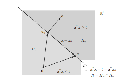
Suppose that $C$ and $D$ are convex sets in $\mathbb{R}^{n}$ and $C \cap D=\emptyset$. Then there exists a hyperplane $H(\mathbf{a}, b)=\left{\mathbf{x} \mid \mathbf{a}^{T} \mathbf{x}=b\right}$ where $\mathbf{a} \in \mathbb{R}^{n}$ is a nonzero vector and $b \in \mathbb{R}$ such that $$ C \subseteq H_{-}(\mathbf{a}, b) \text {, i.e., } \mathbf{a}^{T} \mathbf{x} \leq b, \forall \mathbf{x} \in C $$ and $$ D \subseteq H_{+}(\mathbf{a}, b), \text { i.e., } \mathbf{a}^{T} \mathbf{x} \geq b, \forall \mathbf{x} \in D $$ Only the proof of (2.123) will be given below since the proof of (2.122) can be proven similarly. In the proof, we implicitly assume that the two convex sets $C$ and $D$ are closed without loss of generality. The reasons are that $\mathbf{c l} C$, int $C$, cl $D$, and int $D$ are also convex by Property $2.5$ in Subsection 2.1.4, and thus the same hyperplane that separates $\mathbf{c l} C$ (or int $C$ ) and $\mathbf{c l} D$ (or int $D$ ) can also separate $C$ and $D$. Proof: Let $$ \operatorname{dist}(C, D)=\inf \left{|\mathbf{u}-\mathbf{v}|_{2} \mid \mathbf{v} \in C, \mathbf{u} \in D\right} . $$ Assume that $\operatorname{dist}(C, D)>0$, and that there exists a point $\mathbf{c} \in C$ and a point $\mathbf{d} \in D$ such that $$ |\mathbf{c}-\mathbf{d}|_{2}=\operatorname{dist}(C, D) $$ (as illustrated in Figure $2.20$ ). These assumptions will be satisfied if $C$ and $D$ are closed, and one of $C$ and $D$ is bounded. Note that it is possible that if both $C$ and $D$ are not bounded, such $\mathbf{c} \in C$ and $\mathbf{d} \in D$ may not exist. For instance, $C=\left{(x, y) \in \mathbb{R}^{2} \mid y \geq e^{-x}+1, x \geq 0\right}$ and $D=\left{(x, y) \in \mathbb{R}^{2} \mid y \leq-e^{-x}, x \geq 0\right}$ are convex, closed, and unbounded with $\operatorname{dist}(C, D)=1$, but $\mathbf{c} \in C$ and $\mathbf{d} \in D$ satisfying (2.125) do not exist.
For any nonempty convex set $C$ and for any $\mathbf{x}{0} \in \mathbf{b d} C$, there exists an $\mathbf{a} \neq \mathbf{0}$, such that $\mathbf{a}^{T} \mathbf{x} \leq \mathbf{a}^{T} \mathbf{x}{0}$, for all $\mathbf{x} \in C$; namely, the convex set $C$ is supported by
Proof: Assume that $C$ is a convex set, $A=$ int $C$ (which is open and convex), and $\mathbf{x}{0} \in \mathbf{b d} C$. Let $B=\left{\mathbf{x}{0}\right}$ (which is convex). Then $A \cap B=\emptyset$. By the separating hyperplane theorem, there exists a separating hyperplane $H={\mathbf{x} \mid$ $\left.\mathbf{a}^{T} \mathbf{x}=\mathbf{a}^{T} \mathbf{x}{0}\right}$ (since the distance between the set $A$ and the set $B$ is equal to zero), where $\mathbf{a} \neq \mathbf{0}$, between $A$ and $B$, such that $\mathbf{a}^{T}\left(\mathbf{x}-\mathbf{x}{0}\right) \leq 0$ for all $\mathbf{x} \in C$ (i.e., $C \subseteq H_{-}$by Remark $2.23$ ). Therefore, the hyperplane $H$ is a supporting hyperplane of the convex set $C$ which passes $\mathbf{x}_{0} \in$ bd $C$.
It is now easy to prove, by the supporting hyperplane theorem, that a closed convex set $S$ with int $S \neq \emptyset$ is the intersection of all (possibly an infinite number of) closed halfspaces that contain it (cf. Remark 2.8). Let $$ \mathcal{H}\left(\mathbf{x}{0}\right) \triangleq\left{\mathbf{x} \mid \mathbf{a}^{T}\left(\mathbf{x}-\mathbf{x}{0}\right)=0\right} $$ be a supporting hyperplane of $S$ passing $\mathbf{x}{0} \in \mathbf{b d} S$. This implies, by the hyperplane supporting theorem, that the associated closed halfspace $\mathcal{H}{-}\left(\mathbf{x}{0}\right)$, which contains the closed convex set $S$, is given by $$ \mathcal{H}{-}\left(\mathbf{x}{0}\right) \triangleq\left{\mathbf{x} \mid \mathbf{a}^{T}\left(\mathbf{x}-\mathbf{x}{0}\right) \leq 0\right}, \quad \mathbf{x}{0} \in \mathbf{b d} S $$ Thus it must be true that $$ S=\bigcap{\mathbf{x}{0} \in \mathbf{b d} S} \mathcal{H}{-}\left(\mathbf{x}{0}\right) $$ implying that a closed convex set $S$ can be defined by all of its supporting hyperplanes $\mathcal{H}\left(\mathrm{x}{0}\right)$, though the expression (2.136) may not be unique, thereby justifying Remark $2.8$. When the number of supporting halfspaces containing the closed convex set $S$ is finite, $S$ is a polyhedron. When $S$ is compact and convex,
the supporting hyperplane representation (2.136) can also be expressed as $$ \left.S=\bigcap_{\mathbf{x}{0} \in S{\text {extr }}} \mathcal{H}{-}\left(\mathbf{x}{0}\right) \text { (cf. }(2.24)\right) $$ where the intersection also contains those halfspaces whose boundaries may contain multiple extreme points of $S$. Let us conclude this section with the following three remarks.
数学代写|凸优化作业代写Convex Optimization代考|Summary and discussion
In this chapter, we have introduced convex sets and their properties (mostly geometric properties). Various convexity preserving operations were introduced together with many examples. In addition, the concepts of proper cones on which the generalized equality is defined, dual norms, and dual cones were introduced in detail. Finally, we presented the separating hyperplane theorem, which corroborates the existence of a hyperplane separating two disjoint convex sets, and the existence of the supporting hyperplane of any nonempty convex set. These fundamentals on convex sets along with convex functions to be introduced in the next chapter will be highly instrumental in understanding the concepts of convex optimization. The convex geometry properties introduced in this chapter have been applied to blind hyperspectral unmixing for material identification in remote sensing. Some will be introduced in Chapter 6 .
数学代写|凸优化作业代写Convex Optimization代考|Separating and supporting hyperplanes
If $S_{1}$ and $S_{2}$ are convex sets, then $S_{1} \cap S_{2}$ is also convex. This property extends to the intersection of an infinite number of convex sets, i.e., if $S_{a}$ is convex for every $\alpha \in \mathcal{A}$, then $\cap_{\alpha \in \mathcal{A}} S_{\alpha}$ is convex. Let us illuminate the usefulness of this convexity preserving operation with the following remarks and examples.
Remark 2.6 A polyhedron can be considered as intersection of a finite number of halfspaces and hyperplanes (which are convex) and hence the polyhedron is convex.
Remark 2.7 Subspaces are closed under arbitrary intersections; so are affine sets and convex cones. So they all are convex sets.
Remark 2.8 A closed convex set $S$ is the intersection of all (possibly an infinite number of) closed halfspaces that contain $S$. This can be proven by the separating hyperplane theory (to be introduced in Subsection 2.6.1).
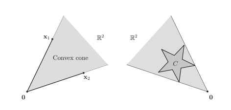
Example 2.4 The PSD cone $\mathbb{S}{+}^{n}$ is known to be convex. The proof of its convexity by the intersection property is given as follows. It is easy to see that $S{+}^{n}$ can be expressed as $$ \mathbb{S}{+}^{n}=\left{\mathbf{X} \in \mathbb{S}^{n} \mid \mathbf{z}^{T} \mathbf{X} \mathbf{z} \geq 0, \forall \mathbf{z} \in \mathbb{R}^{n}\right}=\bigcap{\mathbf{z} \in \mathbb{R}^{n}} S_{\mathbf{z}} $$ where $$ \begin{aligned} S_{\mathbf{z}} &=\left{\mathbf{X} \in \mathbb{S}^{n} \mid \mathbf{z}^{T} \mathbf{X} \mathbf{z} \geq 0\right}=\left{\mathbf{X} \in \mathbb{S}^{n} \mid \operatorname{Tr}\left(\mathbf{z}^{T} \mathbf{X} \mathbf{z}\right) \geq 0\right} \ &=\left{\mathbf{X} \in \mathbb{S}^{n} \mid \operatorname{Tr}\left(\mathbf{X} \mathbf{z z}^{T}\right) \geq 0\right}=\left{\mathbf{X} \in \mathbb{S}^{n} \mid \operatorname{Tr}(\mathbf{X} \mathbf{Z}) \geq 0\right} \end{aligned} $$ in which $\mathbf{Z}=\mathbf{z z}^{T}$, implying that $S_{\mathbf{z}}$ is a halfspace if $\mathbf{z} \neq \mathbf{0}{n}$. As the intersection of halfspaces is also convex, $\mathbb{S}{+}^{n}$ (intersection of infinite number of halfspaces) is a convex set. It is even easier to prove the convexity of $S_{\mathbf{z}}$ by the definition of convex sets. Example 2.5 Consider $$ P(\mathbf{x}, \omega)=\sum_{i=1}^{n} x_{i} \cos (i \omega) $$ and a set $$ \begin{aligned} C &=\left{\mathbf{x} \in \mathbb{R}^{n} \mid l(\omega) \leq P(\mathbf{x}, \omega) \leq u(\omega) \quad \forall \omega \in \Omega\right} \ &=\bigcap_{\omega \in \Omega}\left{\mathbf{x} \in \mathbb{R}^{n} \mid l(\omega) \leq \sum_{i=1}^{n} x_{i} \cos (i \omega) \leq u(\omega)\right} \end{aligned} $$ Let $$ \mathbf{a}(\omega)=[\cos (\omega), \cos (2 \omega), \ldots, \cos (n \omega)]^{T} $$
Then we have $C=\bigcap_{\omega \in \Omega}\left{\mathbf{x} \in \mathbb{R}^{n} \mid \mathbf{a}^{T}(\omega) \mathbf{x} \geq l(\omega), \mathbf{a}^{T}(\omega) \mathbf{x} \leq u(\omega)\right}$ (intersection of halfspaces), which implies that $C$ is convex. Note that the set $C$ is a polyhedron only when the set size $|\Omega|$ is finite.
数学代写|凸优化作业代写Convex Optimization代考|Affine function
A function $f: \mathbb{R}^{n} \rightarrow \mathbb{R}^{m}$ is affine if it takes the form $$ \boldsymbol{f}(\mathbf{x})=\mathbf{A} \mathbf{x}+\mathbf{b} $$ where $\mathbf{A} \in \mathbb{R}^{m \times n}$ and $\mathbf{b} \in \mathbb{R}^{m}$. The affine function, for which $\boldsymbol{f}$ (dom $\boldsymbol{f}$ ) is an affine set if dom $f$ is an affine set, also called the affine transformation or the affine mapping, has been implicitly used in defining the affine hull given by (2.7) in the preceding Subsection 2.1.2. It preserves points, straight lines, and planes, but not necessarily preserves angles between lines or distances between points. The affine mapping plays an important role in a variety of convex sets and convex functions, problem reformulations to be introduced in the subsequent chapters. Suppose $S \subseteq \mathbb{R}^{n}$ is convex and $f: \mathbb{R}^{n} \rightarrow \mathbb{R}^{m}$ is an affine function (see Figure 2.12). Then the image of $S$ under $f$, $$ f(S)={f(\mathbf{x}) \mid \mathbf{x} \in S} $$ is convex. The converse is also true, i.e., the inverse image of the convex set $C$ $$ \boldsymbol{f}^{-1}(C)={\mathbf{x} \mid \boldsymbol{f}(\mathbf{x}) \in C} $$ is convex. The proof is given below. Proof: Let $\mathbf{y}{1}$ and $\mathbf{y}{2} \in C$. Then there exist $\mathbf{x}{1}$ and $\mathbf{x}{2} \in f^{-1}(C)$ such that $\mathbf{y}{1}=\mathbf{A} \mathbf{x}{1}+\mathbf{b}$ and $\mathbf{y}{2}=\mathbf{A} \mathbf{x}{2}+\mathbf{b}$. Our aim is to show that the set $f^{-1}(C)$, which is the inverse image of $\boldsymbol{f}$, is convex. For $\theta \in[0,1]$, $$ \begin{aligned} \theta \mathbf{y}{1}+(1-\theta) \mathbf{y}{2} &=\theta\left(\mathbf{A} \mathbf{x}{1}+\mathbf{b}\right)+(1-\theta)\left(\mathbf{A \mathbf { x } { 2 }}+\mathbf{b}\right) \ &=\mathbf{A}\left(\theta \mathbf{x}{1}+(1-\theta) \mathbf{x}{2}\right)+\mathbf{b} \in C \end{aligned} $$ which implies that $\theta \mathbf{x}{1}+(1-\theta) \mathbf{x}{2} \in f^{-1}(C)$, and that the convex combination of $\mathbf{x}{1}$ and $\mathbf{x}{2}$ is in $f^{-1}(C)$, and hence $f^{-1}(C)$ is convex.
Remark 2.9 If $S_{1} \subset \mathbb{R}^{n}$ and $S_{2} \subset \mathbb{R}^{n}$ are convex and $\alpha_{1}, \alpha_{2} \in \mathbb{R}$, then the set $S=\left{(\mathbf{x}, \mathbf{y}) \mid \mathbf{x} \in S_{1}, \mathbf{y} \in S_{2}\right}$ is convex. Furthermore, the set $$ \alpha_{1} S_{1}+\alpha_{2} S_{2}=\left{\mathbf{z}=\alpha_{1} \mathbf{x}+\alpha_{2} \mathbf{y} \mid \mathbf{x} \in S_{1}, \mathbf{y} \in S_{2}\right} \quad(\text { cf. (1.22) and (1.23)) } $$ is also convex (since this set can be thought of as the image of the convex set $S$ through the affine mapping given by (2.58) from $S$ to $\alpha_{1} S_{1}+\alpha_{2} S_{2}$ with
数学代写|凸优化作业代写Convex Optimization代考|Perspective function and linear-fractional function
Linear-fractional functions are functions which are more general than affine but still preserve convexity. The perspective function scales or normalizes vectors so that the last component is one, and then drops the last component.
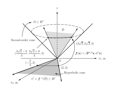
The perspective function $\boldsymbol{p}: \mathbb{R}^{n+1} \rightarrow \mathbb{R}^{n}$, with $\operatorname{dom} \boldsymbol{p}=\mathbb{R}^{n} \times \mathbb{R}{++}$, is defined as $$ \boldsymbol{p}(\mathbf{z}, t)=\frac{\mathbf{z}}{t} . $$ The perspective function $\boldsymbol{p}$ preserves the convexity of the convex set. Proof: Consider two points $\left(\mathbf{z}{1}, t_{1}\right)$ and $\left(\mathbf{z}{2}, t{2}\right)$ in a convex set $C$ and so $\mathbf{z}{1} / t{1}$ and $\mathbf{z}{2} / t{2} \in \boldsymbol{p}(C)$. Then $$ \theta\left(\mathbf{z}{1}, t{1}\right)+(1-\theta)\left(\mathbf{z}{2}, t{2}\right)=\left(\theta \mathbf{z}{1}+(1-\theta) \mathbf{z}{2}, \theta t_{1}+(1-\theta) t_{2}\right) \in C, $$ for any $\theta \in[0,1]$ implying $$ \frac{\theta \mathbf{z}{1}+(1-\theta) \mathbf{z}{2}}{\theta t_{1}+(1-\theta) t_{2}} \in \boldsymbol{p}(C) $$ Now, by defining $$ \mu=\frac{\theta t_{1}}{\theta t_{1}+(1-\theta) t_{2}} \in[0,1], $$ we get $$ \frac{\theta \mathbf{z}{1}+(1-\theta) \mathbf{z}{2}}{\theta t_{1}+(1-\theta) t_{2}}=\mu \frac{\mathbf{z}{1}}{t{1}}+(1-\mu) \frac{\mathbf{z}{2}}{t{2}} \in \boldsymbol{p}(C), $$ which implies $\boldsymbol{p}(C)$ is convex. A linear-fractional function is formed by composing the perspective function with an affine function. Suppose $\boldsymbol{g}: \mathbb{R}^{n} \rightarrow \mathbb{R}^{m+1}$ is affine, i.e., $$ \boldsymbol{g}(\mathbf{x})=\left[\begin{array}{c} \mathbf{A} \ \mathbf{c}^{T} \end{array}\right] \mathbf{x}+\left[\begin{array}{l} \mathbf{b} \ d \end{array}\right] $$
where $\mathbf{A} \in \mathbb{R}^{m \times n}, \mathbf{b} \in \mathbb{R}^{m}, \mathbf{c} \in \mathbb{R}^{n}$, and $d \in \mathbb{R}$. The function $\boldsymbol{f}: \mathbb{R}^{n} \rightarrow \mathbb{R}^{m}$ is given by $f=\boldsymbol{p} \circ \boldsymbol{g}$, i.e., $$ \boldsymbol{f}(\mathbf{x})=\boldsymbol{p}(\boldsymbol{g}(\mathbf{x}))=\frac{\mathbf{A} \mathbf{x}+\mathbf{b}}{\mathbf{c}^{T} \mathbf{x}+d}, \quad \operatorname{dom} \boldsymbol{f}=\left{\mathbf{x} \mid \mathbf{c}^{T} \mathbf{x}+d>0\right}, $$ is called a linear-fractional (or projective) function. Hence, linear-fractional functions preserve the convexity.
数学代写|凸优化作业代写Convex Optimization代考|Examples of convex sets
数学代写|凸优化作业代写Convex Optimization代考|Hyperplanes and halfspaces
A hyperplane is an affine set (hence a convex set) and is of the form $$ H=\left{\mathbf{x} \mid \mathbf{a}^{T} \mathbf{x}=b\right} \subset \mathbb{R}^{n}, $$ where $\mathbf{a} \in \mathbb{R}^{n} \backslash\left{\mathbf{0}_{n}\right}$ is a normal vector of the hyperplane, and $b \in \mathbb{R}$. Analytically it is the solution set of a linear equation of the components of $\mathbf{x}$. In geometrical sense, a hyperplane can be interpreted as the set of points having a constant inner product (b) with the normal vector (a). Since affdim $(H)=n-1$,
the hyperplane (2.30) can also be expressed as $$ H=\operatorname{aff}\left{\mathbf{s}{1}, \ldots, \mathbf{s}{n}\right} \subset \mathbb{R}^{n}, $$ where $\left{\mathbf{s}{1}, \ldots, \mathbf{s}{n}\right} \subset H$ is any affinely independent set. Then it can be seen that $$ \left{\begin{array}{l} \mathbf{B} \triangleq\left[\mathbf{s}{2}-\mathbf{s}{1}, \ldots, \mathbf{s}{n}-\mathbf{s}{1}\right] \in \mathbb{R}^{n \times(n-1)} \text { and } \operatorname{dim}(\mathcal{R}(\mathbf{B}))=n-1 \ \mathbf{B}^{T} \mathbf{a}=\mathbf{0}{n-1}, \text { i.e. }, \mathcal{R}(\mathbf{B})^{\perp}=\mathcal{R}(\mathbf{a}) \end{array}\right. $$ implying that the normal vector a can be determined from $\left{\mathbf{s}{1}, \ldots, \mathbf{s}_{n}\right}$ up to a scale factor.
The hyperplane $H$ defined in $(2.30)$ divides $\mathbb{R}^{n}$ into two closed halfspaces as follows: $$ \begin{aligned} &H_{-}=\left{\mathbf{x} \mid \mathbf{a}^{T} \mathbf{x} \leq b\right} \ &H_{+}=\left{\mathbf{x} \mid \mathbf{a}^{T} \mathbf{x} \geq b\right} \end{aligned} $$ and so each of them is the solution set of one (non-trivial) linear inequality. Note that $\mathbf{a}=\nabla\left(\mathbf{a}^{T} \mathbf{x}\right)$ denotes the maximally increasing direction of the linear function $\mathbf{a}^{T} \mathbf{x}$. The above representations for both $H_{-}$and $H_{+}$for a given $\mathbf{a} \neq \mathbf{0}$, are not unique, while they are unique if $\mathbf{a}$ is normalized such that $|\mathbf{a}|_{2}=1$. Moreover, $H_{-} \cap H_{+}=H$. An open halfspace is a set of the form $$ H_{–}=\left{\mathbf{x} \mid \mathbf{a}^{T} \mathbf{x}b\right} $$ where $\mathbf{a} \in \mathbb{R}^{n}, \mathbf{a} \neq \mathbf{0}$, and $b \in \mathbb{R}$.
数学代写|凸优化作业代写Convex Optimization代考|Euclidean balls and ellipsoids
A Euclidean ball (or, simply, ball) in $\mathbb{R}^{n}$ has the following form: $$ B\left(\mathbf{x}{c}, r\right)=\left{\mathbf{x} \mid\left|\mathbf{x}-\mathbf{x}{c}\right|_{2} \leq r\right}=\left{\mathbf{x} \mid\left(\mathbf{x}-\mathbf{x}{c}\right)^{T}\left(\mathbf{x}-\mathbf{x}{c}\right) \leq r^{2}\right}, $$ where $r>0$. The vector $\mathbf{x}{c}$ is the center of the ball and the positive scalar $r$ is its radius (see Figure 2.7). The Euclidean ball is also a 2-norm ball, and, for simplicity, a ball without explicitly mentioning the associated norm, means the Euclidean ball hereafter. Another common representation for the Euclidean ball is $$ B\left(\mathbf{x}{c}, r\right)=\left{\mathbf{x}{c}+r \mathbf{u} \mid|\mathbf{u}|{2} \leq 1\right} $$ It can be easily proved that the Euclidean ball is a convex set. Proof of convexity: Let $\mathbf{x}{1}$ and $\mathbf{x}{2} \in B\left(\mathbf{x}{c}, r\right)$, i.e., $\left|\mathbf{x}{1}-\mathbf{x}{c}\right|{2} \leq r$ and $| \mathbf{x}{2}-$ $\mathbf{x}{c} |_{2} \leq r$. Then, $$ \begin{aligned} \left|\theta \mathbf{x}{1}+(1-\theta) \mathbf{x}{2}-\mathbf{x}{c}\right|{2} &=\left|\theta \mathbf{x}{1}+(1-\theta) \mathbf{x}{2}-\left[\theta \mathbf{x}{c}+(1-\theta) \mathbf{x}{c}\right]\right|_{2} \ &=\left|\theta\left(\mathbf{x}{1}-\mathbf{x}{c}\right)+(1-\theta)\left(\mathbf{x}{2}-\mathbf{x}{c}\right)\right|_{2} \ & \leq\left|\theta\left(\mathbf{x}{1}-\mathbf{x}{c}\right)\right|_{2}+\left|(1-\theta)\left(\mathbf{x}{2}-\mathbf{x}{c}\right)\right|_{2} \ & \leq \theta r+(1-\theta) r \ &=r, \text { for all } 0 \leq \theta \leq 1 \end{aligned} $$ Hence, $\theta \mathbf{x}{1}+(1-\theta) \mathbf{x}{2} \in B\left(\mathbf{x}{c}, r\right)$ for all $\theta \in[0,1]$, and thus we have proven that $B\left(\mathbf{x}{c}, r\right)$ is convex.
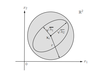
A related family of convex sets are ellipsoids (see Figure $2.7$ ), which have the form $$ \mathcal{E}=\left{\mathbf{x} \mid\left(\mathbf{x}-\mathbf{x}{c}\right)^{T} \mathbf{P}^{-1}\left(\mathbf{x}-\mathbf{x}{c}\right) \leq 1\right}, $$ where $\mathbf{P} \in \mathcal{S}{++}^{n}$ and the vector $\mathbf{x}{c}$ is the center of the ellipsoid. The matrix $\mathbf{P}$ determines how far the ellipsoid extends in every direction from the center; the lengths of the semiaxes of $\mathcal{E}$ are given by $\sqrt{\lambda_{i}}$, where $\lambda_{i}$ are eigenvalues of $\mathbf{P}$. Note that a ball is an ellipsoid with $\mathbf{P}=r^{2} \mathbf{I}{n}$ where $r>0$. Another common representation of an ellipsoid is $$ \mathcal{E}=\left{\mathbf{x}{c}+\mathbf{A u} \mid|\mathbf{u}|_{2} \leq 1\right} $$ where $\mathbf{A}$ is a square matrix and nonsingular. The ellipsoid $\mathcal{E}$ expressed by (2.38) is actually the image of the 2 -norm ball $B(\mathbf{0}, 1)=\left{\mathbf{u} \in \mathbb{R}^{n} \mid|\mathbf{u}|_{2} \leq 1\right}$ via an
affine mapping $\mathbf{x}{c}+\mathbf{A u}$ (cf. $\left.(2.58)\right)$, where $\mathbf{A}=\left(\mathbf{P}^{1 / 2}\right)^{T}$, and the proof will be presented below. With the expression (2.38) for an ellipsoid, the singular values of $\mathbf{A}, \sigma{i}(\mathbf{A})=\sqrt{\lambda_{i}}$ (lengths of semiaxes) characterize the structure of the ellipsoid in a more straightforward fashion than the expression (2.37). Proof of the ellipsoid representation (2.38) and convexity: Let $$ \mathbf{P}=\mathbf{Q} \boldsymbol{\Lambda} \mathbf{Q}^{T}=\left(\mathbf{P}^{1 / 2}\right)^{T} \mathbf{P}^{1 / 2} $$ $(\mathrm{EVD}$ of $\mathbf{P} \succ \mathbf{0})$, where $\boldsymbol{\Lambda}=\boldsymbol{\operatorname { D i a g }}\left(\lambda_{1}, \lambda_{2}, \ldots, \lambda_{n}\right)$ and $$ \mathbf{P}^{1 / 2}=\boldsymbol{\Lambda}^{1 / 2} \mathbf{Q}^{T}, $$ in which $\Lambda^{1 / 2}=\operatorname{Diag}\left(\sqrt{\lambda_{1}}, \sqrt{\lambda_{2}}, \ldots, \sqrt{\lambda_{n}}\right)$. Then $$ \mathbf{P}^{-1}=\mathbf{Q} \boldsymbol{\Lambda}^{-1} \mathbf{Q}^{T}=\mathbf{P}^{-1 / 2}\left(\mathbf{P}^{-1 / 2}\right)^{T}, \quad \mathbf{P}^{-1 / 2}=\mathbf{Q} \mathbf{\Lambda}^{-1 / 2} $$ From the definition of ellipsoid, we have $$ \begin{aligned} \mathcal{E} &=\left{\mathbf{x} \mid\left(\mathbf{x}-\mathbf{x}{c}\right)^{T} \mathbf{P}^{-1}\left(\mathbf{x}-\mathbf{x}{c}\right) \leq 1\right} \ &=\left{\mathbf{x} \mid\left(\mathbf{x}-\mathbf{x}{c}\right)^{T} \mathbf{Q} \mathbf{\Lambda}^{-1} \mathbf{Q}^{T}\left(\mathbf{x}-\mathbf{x}{c}\right) \leq 1\right} \end{aligned} $$ Let $\mathbf{z}=\mathbf{x}-\mathbf{x}{c}$. Then $$ \mathcal{E}=\left{\mathbf{x}{c}+\mathbf{z} \mid \mathbf{z}^{T} \mathbf{Q} \mathbf{\Lambda}^{-1} \mathbf{Q}^{T} \mathbf{z} \leq 1\right} $$ Now, by letting $\mathbf{u}=\mathbf{\Lambda}^{-1 / 2} \mathbf{Q}^{T} \mathbf{z}=\left(\mathbf{P}^{-1 / 2}\right)^{T} \mathbf{z}$, we then obtain $$ \mathcal{E}=\left{\mathbf{x}{c}+\left(\mathbf{P}^{1 / 2}\right)^{T} \mathbf{u} \mid|\mathbf{u}|{2} \leq 1\right} $$ which is exactly (2.38) with $\left(\mathbf{P}^{1 / 2}\right)^{T}$ replaced by $\mathbf{A}$.
数学代写|凸优化作业代写Convex Optimization代考|Polyhedra
A polyhedron is a nonempty convex set and is defined as the solution set of a finite number of linear equalities and inequalities: $$ \begin{aligned} \mathcal{P} &=\left{\mathbf{x} \mid \mathbf{a}{i}^{T} \mathbf{x} \leq b{i}, i=1,2, \ldots, m, \mathbf{c}{j}^{T} \mathbf{x}=d{j}, j=1,2, \ldots, p\right} \ &=\left{\mathbf{x} \mid \mathbf{A} \mathbf{x} \preceq \mathbf{b}=\left(b_{1}, \ldots, b_{m}\right), \mathbf{C x}=\mathbf{d}=\left(d_{1}, \ldots, d_{p}\right)\right} \end{aligned} $$ where ” $\preceq “$ stands for componentwise inequality, $\mathbf{A} \in \mathbb{R}^{m \times n}$ and $\mathbf{C} \in \mathbb{R}^{p \times n}$ are matrices whose rows are $\mathbf{a}{j}^{T} \mathrm{~s}$ and $\mathbf{c}{j}^{T} \mathrm{~s}$, respectively, and $\mathbf{A} \neq \mathbf{0}$ or $\mathbf{C} \neq \mathbf{0}$ must be true. Note that either $m=0$ or $p=0$ is allowed as long as the other parameter is finite and nonzero.
A polyhedron is just the intersection of some halfspaces and hyperplanes (see Figure 2.8). A polyhedron can be unbounded, while a bounded polyhedron is called a polytope, e.g., any 1-norm ball and $\infty$-norm ball of finite radius are polytopes.
Remark 2.3 It can be seen that the $\ell$-dimensional space $\mathbb{R}^{\ell}$ (also an affine set) cannot be expressed in the standard form (2.41) with either nonzero $\mathbf{A}$ or nonzero $\mathbf{C}$, and so it is not a polyhedron for any $\ell \in \mathbb{Z}{++}$. However, because any affine set in $\mathbb{R}^{\ell}$ can be expressed as (2.7) and each $\mathbf{x}$ in the set satisfies (2.8), this implies that the affine set must be a polyhedron if its affine dimension is strictly less than $\ell$. For instance, any subspaces with dimension less than $n$ in $\mathbb{R}^{n}$, and any hyperplane that is defined by a normal vector $\mathbf{a} \neq \mathbf{0}$ and a point $\mathbf{x}{0}$ on the hyperplane, i.e., $$ \mathcal{H}\left(\mathbf{a}, \mathbf{x}{0}\right)=\left{\mathbf{x} \mid \mathbf{a}^{T}\left(\mathbf{x}-\mathbf{x}{0}\right)=0\right}=\left{\mathbf{x}_{0}\right}+\mathcal{R}(\mathbf{a})^{\perp} $$ in $\mathbb{R}^{n}$, and rays, line segments, and halfspaces are all polyhedra.
数学代写|凸优化作业代写Convex Optimization代考|Examples of convex sets
数学代写|凸优化作业代写Convex Optimization代考|Summary and discussion
数学代写|凸优化作业代写Convex Optimization代考|Summary and discussion
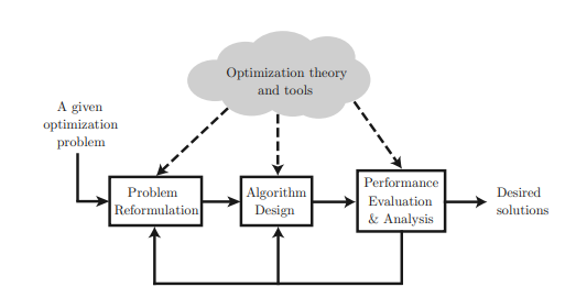
In this chapter, we have revisited some mathematical basics of sets, functions, matrices, and vector spaces that will be very useful to understand the remaining chapters and we also introduced the notations that will be used throughout this book. The mathematical preliminaries reviewed in this chapter are by no means complete. For further details, the readers can refer to [Apo07] and [WZ97] for Section 1.1, and [H.J85] and [MS00] for Section 1.2, and other related textbooks. Suppose that we are given an optimization problem in the following form: $$ \begin{aligned} \text { minimize } & f(\boldsymbol{x}) \ \text { subject to } & \boldsymbol{x} \in \mathcal{C} \end{aligned} $$ where $f(\boldsymbol{x})$ is the objective function to be minimized and $\mathcal{C}$ is the feasible set from which we try to find an optimal solution. Convex optimization itself is a powerful mathematical tool for optimally solving a well-defined convex optimization problem (i.e., $f(\boldsymbol{x})$ is a convex function and $\mathcal{C}$ is a convex set in problem $(1.127)$ ), or for handling a nonconvex optimization problem (that can be approximated as a convex one). However, the problem (1.127) under investigation may often appear to be a nonconvex optimization problem (with various camouflages) or a nonconvex and nondeterministic polynomial-time hard (NP-hard) problem that forces us to find an approximate solution with some performance or computational efficiency merits and characteristics instead. Furthermore, reformulation of the considered optimization problem into a convex optimization problem can be quite challenging. Fortunately, there are many problem reformulation approaches (e.g., function transformation, change of variables, and equivalent representations) to conversion of a nonconvex problem into a convex problem (i.e., unveiling of all the camouflages of the original problem).
The bridge between the pure mathematical convex optimization theory and how to use it in practical applications is the key for a successful researcher or professional who can efficiently exert his (her) efforts on solving a challenging scientific and engineering problem to which he (she) is dedicated. For a given opti-
mization problem, we aim to design an algorithm (e.g., transmit beamforming algorithm and resource allocation algorithm in communications and networking, nonnegative blind source separation algorithm for the analysis of biomedical and hyperspectral images) to efficiently and reliably yield a desired solution (that may just be an approximate solution rather than an optimal solution), as shown in Figure 1.6, where the block “Problem Reformulation,” the block “Algorithm Design,” and the block “Performance Evaluation and Analysis” are essential design steps before an algorithm that meets our goal is obtained. These design steps rely on smart use of advisable optimization theory and tools that remain in the cloud, like a military commander who needs not only ammunition and weapons but also an intelligent fighting strategy. It is quite helpful to build a bridge so that one can readily use any suitable mathematical theory (e.g., convex sets and functions, optimality conditions, duality, KKT conditions, Schur complement, S-procedure, etc.) and convex solvers (e.g., CVX and SeDuMi) to accomplish these design steps.
The ensuing chapters will introduce fundamental elements of the convex optimization theory in the cloud on one hand and illustrate how these elements were collectively applied in some successful cutting edge researches in communications and signal processing through the design procedure shown in Figure $1.6$ on the other hand, provided that the solid bridges between the cloud and all the design blocks have been constructed.
数学代写|凸优化作业代写Convex Optimization代考|Lines and line segments
In this chapter we introduce convex sets and their representations, properties, illustrative examples, convexity preserving operations, and geometry of convex sets which have proven very useful in signal processing applications such as hyperspectral and biomedical image analysis. Then we introduce proper cones (convex cones), dual norms and dual cones, generalized inequalities, and separating and supporting hyperplanes. All the materials on convex sets introduced in this chapter are essential to convex functions, convex problems, and duality to be introduced in the ensuing chapters. From this chapter on, for simplicity, we may use $\mathbf{x}$ to denote a vector in $\mathbb{R}^{n}$ and $x_{1}, \ldots, x_{n}$ for its components without explicitly mentioning $\mathbf{x} \in \mathbb{R}^{n}$.
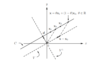
Mathematically, a line $\mathcal{L}\left(\mathbf{x}{1}, \mathbf{x}{2}\right)$ passing through two points $\mathbf{x}{1}$ and $\mathbf{x}{2}$ in $\mathbb{R}^{n}$ is the set defined as $$ \mathcal{L}\left(\mathbf{x}{1}, \mathbf{x}{2}\right)=\left{\theta \mathbf{x}{1}+(1-\theta) \mathbf{x}{2}, \theta \in \mathbb{R}\right}, \mathbf{x}{1}, \mathbf{x}{2} \in \mathbb{R}^{n} $$ If $0 \leq \theta \leq 1$, then it is a line segment connecting $\mathbf{x}{1}$ and $\mathbf{x}{2}$. Note that the linear combination $\theta \mathbf{x}{1}+(1-\theta) \mathbf{x}{2}$ of two points $\mathbf{x}{1}$ and $\mathbf{x}{2}$ with the coefficient sum equal to unity as in (2.1) plays an essential role in defining affine sets and convex sets, and hence the one with $\theta \in \mathbb{R}$ is referred to as the affine combination and the one with $\theta \in[0,1]$ is referred to as the convex combination. Affine combination and convex combination can be extended to the case of more than two points in the same fashion. Affine sets and affine hulls A set $C$ is said to be an affine set if for any $\mathbf{x}{1}, \mathbf{x}{2} \in C$ and for any $\theta_{1}, \theta_{2} \in \mathbb{R}$ such that $\theta_{1}+\theta_{2}=1$, the point $\theta_{1} \mathbf{x}{1}+\theta{2} \mathbf{x}_{2}$ also belongs to the set $C$. For instance, the line defined in $(2.1)$ is an affine set. This concept can be extended to more than two points, as illustrated in the following example.
数学代写|凸优化作业代写Convex Optimization代考|Relative interior and relative boundary
Affine hull defined in (2.13) and affine dimension of a set defined in (2.14) play an essential role in convex geometric analysis, and have been applied to dimension reduction in many signal processing applications such as blind separation (or unmixing) of biomedical and hyperspectral image signals (to be introduced in Chapter 6). To further illustrate their characteristics, it would be useful to address the interior and the boundary of a set w.r.t. its affine hull, which are, respectively, termed as relative interior and relative boundary, and are defined below.
The relative interior of $C \subseteq \mathbb{R}^{n}$ is defined as $$ \text { relint } \begin{aligned} C &={\mathbf{x} \in C \mid B(\mathbf{x}, r) \cap \text { aff } C \subseteq C, \text { for some } r>0} \ &=\text { int } C \text { if aff } C=\mathbb{R}^{n} \quad(c f .(1.20)), \end{aligned} $$ where $B(\mathbf{x}, r)$ is a 2 -norm ball with center at $\mathbf{x}$ and radius $r$. It can be inferred from (2.16) that $$ \text { int } C= \begin{cases}\text { relint } C, & \text { if affdim } C=n \ 0, & \text { otherwise. }\end{cases} $$ The relative boundary of a set $C$ is defined as $$ \begin{aligned} \text { relbd } C &=\mathbf{c l} C \backslash \text { relint } C \ &=\mathbf{b d} C \text {, if int } C \neq \emptyset \text { (by }(2.17)) \end{aligned} $$ For instance, for $C=\left{\mathbf{x} \in \mathbb{R}^{n} \mid|\mathbf{x}|_{\infty} \leq 1\right}$ (an infinity-norm ball), its interior and relative interior are identical, so are its boundary and relative boundary; for $C=\left{\mathbf{x}_{0}\right} \subset \mathbb{R}^{n}$ (a singleton set), int $C=\emptyset$ and bd $C=C$, but relbd $C=\emptyset$. Note that affdim $(C)=n$ for the former but affdim $(C)=0 \neq n$ for the latter, thereby providing the information of differentiating the interior (boundary) and the relative interior (relative boundary) of a set. Some more examples about the relative interior (relative boundary) of $C$ and the interior (boundary) of $C$, are illustrated in the following examples.
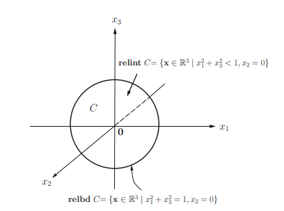
Example 2.2 Let $C=\left{\mathrm{x} \in \mathbb{R}^{3} \mid x_{1}^{2}+x_{3}^{2} \leq 1, x_{2}=0\right}=\mathrm{cl} C$. Then relint $C=$ $\left{\mathbf{x} \in \mathbb{R}^{3} \mid x_{1}^{2}+x_{3}^{2}<1, x_{2}=0\right}$ and relbd $C=\left{\mathbf{x} \in \mathbb{R}^{3} \mid x_{1}^{2}+x_{3}^{2}=1, x_{2}=0\right}$ as shown in Figure $2.3$. Note that int $C=\emptyset$ since affdim $(C)=2<3$, while bd $C=$ cl $C \backslash$ int $C=C$.
Example $2.3$ Let $C_{1}=\left{\mathbf{x} \in \mathbb{R}^{3} \mid|\mathbf{x}|_{2} \leq 1\right}$ and $C_{2}=\left{\mathbf{x} \in \mathbb{R}^{3} \mid|\mathbf{x}|_{2}=1\right}$. Then int $C_{1}=\left{\mathbf{x} \in \mathbb{R}^{3} \mid|\mathbf{x}|_{2}<1\right}=$ relint $C_{1}$ and int $C_{2}=$ relint $C_{2}=0$ due to $\operatorname{affdim}\left(C_{1}\right)=\operatorname{affdim}\left(C_{2}\right)=3$.
From now on, for the conceptual conciseness and clarity in the following introduction to convex sets, sometimes we address the pair (int $C$, bd $C$ ) in the context without explicitly mentioning that a convex set $C$ has nonempty interior. However, when int $C=\emptyset$ in the context, one can interpret the pair (int $C$, bd $C$ ) as the pair (relint $C$, relbd $C$ ).
数学代写|凸优化作业代写Convex Optimization代考|Summary and discussion