EGN2440 - 统计代写答疑辅导

标签： EGN2440

统计代写|工程统计作业代写Engineering Statistics代考|Values of Distributions and Inverses

Posted on 2022年5月19日2022年5月19日 by statistics-lab

如果你也在怎样代写工程统计Engineering Statistics这个学科遇到相关的难题，请随时右上角联系我们的24/7代写客服。

工程统计结合了工程和统计，使用科学方法分析数据。工程统计涉及有关制造过程的数据，如：部件尺寸、公差、材料类型和制造过程控制。

statistics-lab™ 为您的留学生涯保驾护航在代写工程统计Engineering Statistics方面已经树立了自己的口碑, 保证靠谱, 高质且原创的统计Statistics代写服务。我们的专家在代写工程统计Engineering Statistics代写方面经验极为丰富，各种代写工程统计Engineering Statistics相关的作业也就用不着说。

我们提供的工程统计Engineering Statistics及其相关学科的代写，服务范围广, 其中包括但不限于:

Statistical Inference 统计推断
Statistical Computing 统计计算
Advanced Probability Theory 高等概率论
Advanced Mathematical Statistics 高等数理统计学
(Generalized) Linear Models 广义线性模型
Statistical Machine Learning 统计机器学习
Longitudinal Data Analysis 纵向数据分析
Foundations of Data Science 数据科学基础

统计代写|工程统计作业代写Engineering Statistics代考|“Student’s” t-Distribution

统计代写|工程统计作业代写Engineering Statistics代考|For Continuum-Valued Variables

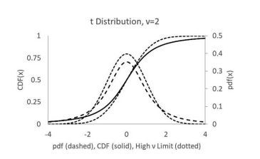
For continuum-valued variables, $x$, the cumulative distribution function is the probability of getting a particular value or a lower value of a variable. It is the left-sided area on the probability density curve, often expressed as alpha. It is variously represented as $C D F(x)=F(x)=\alpha=p$. Here we ll use the $C D F(x)$ notation.

For continuous-valued variables, $x$, the probability distribution function, $p d f(x)$, represents the rate of increase of probability of occurrence of the value $x$. An alternate notation is $p d f(x)=f(x)$.

The relation between CDF(x) and $p d f(x)$ is
$$
\operatorname{CDF}(x)=\int_{x_{\text {mimeme }}}^{x} p d f(x) d x
$$
Where $x_{\text {minimun }}$ represents the lowest possible value for $x$. In a normal distribution $x_{\operatorname{minimum}}=$ $-\infty$. For a chi-squared distribution $x_{\text {minimun }}=0$.

The left-hand sketch in Figure $3.16$ illustrates the $C D F$ and the right-hand sketch the $p d f$ of $z$ for a standard normal distribution (the mean is zero and the standard deviation is unity). At a value of $z=-1$, the $C D F$ is about $0.158$, and the rate of increase of the $C D F$, the $p d f$ is about $0.242$. The notations are $0.158=C D F(-1)$ and $0.242=p d f(-1)$. In both you enter the graph on the horizontal axis, the $z$-value, and read the value on the vertical axis.

For continuous-valued variables the inverse of the CDF is the value of $x$ for which the probability of getting the value of $x$ or a lower value is equal to the CDF $(x)$.

The inverse would enter on the vertical axis to read the value on the horizontal axis. If the inverse question is, “What $z$-value marks the point for which equal or lower $z$-values have a probability of $0.158$ of occurring?” then we represent this inverse question as $z=\operatorname{CDF}^{-1}(\alpha)$. In this illustration, $-1=\operatorname{CDF}^{-1}(0.158)$. The inverse of the right-hand $p d f$ graph is not unique. If the question is to determine the $z$-value for which the $p d f=0.242$, there are two values, $z=-1$, and $z=+1$.

统计代写|工程统计作业代写Engineering Statistics代考|For Discrete-Valued Variables

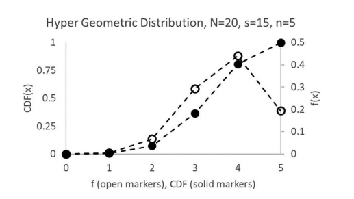
For discrete-valued variables, $x$, likely a count of the number of events, the cumulative distribution function is the probability of getting a particular value or a lower value of a variable. It is the left-sided area on the probability density curve, often expressed as alpha. It is variously represented as $\operatorname{CDF}(x)=F(x)=\alpha=p$. Again, we will use the $C D F(x)$ notation.
For discrete-valued variables, $x$, the point distribution function, $p d f(x)$, represents the probability of an occurrence of the value $x$. An alternate notation is $p d f(x)=f(x)$. Here, $p d f(x)$ is a probability of a particular value of $x$, not the rate that the CDF is increasing. Unfortunately, the same symbol is used in continuum-valued distribution.
The relation between $\operatorname{CDF}(x)$ and $p d f(x)$ is
$$
\operatorname{CDF}(x)=\sum_{x_{\text {meimum }}}^{x} p d f(x)
$$

where $x_{\text {minimum }}$ represents the lowest possible value for $x$. Normally $x_{\text {minimum }}=0$, the least number of events that could occur.

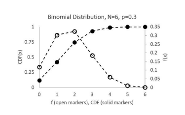
The left-hand sketch of Figure $3.17$ illustrates the CDF and the right-hand sketch the $p d f$ of $s$, the count of the number of successes, for a binomial distribution (the number of trials is 40 , and the probability of success on any particular trial is $0.3$ ). Note that the markers on the graphs represent feasible values. The light line connecting the dots is a visual convenience. It is not possible to have $10.3$ successes. At a value of $s=10$, the CDF is about $0.309$, meaning that there is about a $31 \%$ chance of getting 10 or fewer successes. The $p d f$ is about $0.113$, meaning that the probability of getting exactly 10 successes is about $11 \%$. The notations are $0.309=\operatorname{CDF}(10)$ and $0.113=p d f(10)$. In both you enter the graph on the horizontal axis, the $s$-value, and read the value on the vertical axis.

For discrete-valued variables the inverse of the $C D F$ is the value of $s$ for which the probability of getting the value of $s$ or a lower value is equal to the CDF(s).
The inverse would enter on the vertical axis to read the value on the horizontal axis. If the inverse question is, “What $s$-value marks the point for which equal or lower counts have a probability of $0.309$ of occurring?” then we represent this inverse question as $s=C D F^{-1}(\alpha)$. In this illustration, $10=C D F^{-1}(0.309)$. The inverse of the right-hand pdf graph appears to be not unique. However, it might be. If the question is to determine the s-value for which the $p d f=0.113$, there is only one value, $s=10$. It appears that an $s$-value of about $13.5$ could have such a CDF value, but the count must be an integer. The $p d f$ of $S=13$ is $0.126$, and the $p d f$ of $S=14$ is $0.104$.

Although one could ask, “What count value, or lower, has a $30 \%$ chance of occurring?” it is impossible to match the $30 \% C D F=0.3 \overline{000}$ value. $S \leq 9$ has a $C D F$ of about $0.196$ which does not include the target $0.3 \overline{000} . S \leq 10$ has a CDF of about $0.309$ which does match. $S=10$ is the lowest value that includes the target $C D F$. One convention is to report the minimum count that includes the target $C D F$ value.

统计代写|工程统计作业代写Engineering Statistics代考|Propagating Distributions with Variable Transformations

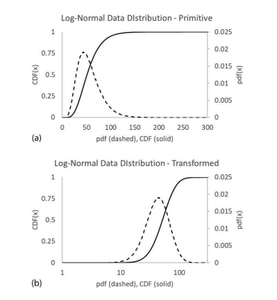
Often, we know the distribution on $x$-values and have a model that transforms $x$ to $y$. For instance, $y=\operatorname{Ln}(x)$. The question is, “What is the distribution of $y$ ?”

Figure $3.18$ reveals the case of $y=a+b x^{3}$ when the distribution on $x$ (on the abscissa) is normal.

Note: For the range of $x$-values shown, the function is strictly monotonic, positive definite. As $x$ increases, $y$ increases for all values of $x$. There are no places in the $x$-range where either 1) the derivative is negative or 2) zero (there are no flat spots in the function).

The inset sketches indicate the $p d f$ (dashed line) and CDF of $x$ and $y$, about a nominal value of $x_{0}=2.5$ and the corresponding $y_{0}=a+b x_{0}{ }^{3}$. Note that the $p d f$ of $x$ is symmetric, and that of $y$ is skewed.

The CDF of $x$ indicates the probability that $x$ could have a lower value. For any $x$ there is a corresponding $y$, and since the function is strictly monotonic, the probability of a lower $y$-value is the same as the probability of a lower $y$-value. Then
$$
\operatorname{CDF}(y=f(x))=\operatorname{CDF}(x)
$$
Between any two corresponding points $x_{1}$ and $x_{2}$ separated by $\Delta x=x_{2}-x_{1}$, there are the two corresponding points $y_{1}=f\left(x_{1}\right)$ and $y_{2}=f\left(x_{2}\right)$ separated by $\Delta y=f\left(x_{2}\right)-f\left(x_{1}\right) \cong \frac{d y}{d x} \Delta x$ for small $\Delta x$ values (meaning that $\frac{d y}{d x}$ is relatively unchanged over the $\Delta x$ interval). Since $\operatorname{CDF}\left(y_{2}\right)=\operatorname{CDF}\left(x_{2}\right)$ and $\operatorname{CDF}\left(y_{1}\right)=\operatorname{CDF}\left(x_{1}\right)$, the difference is also equal, and by definition:
$$
\int_{y_{1}}^{y_{2}} p d f(y) d y=\int_{x_{1}}^{x_{2}} p d f(x) d x
$$
For small $\Delta x$ intervals, the integral can be approximated by the trapezoid rule of integration, and in the limit of very small $\Delta x$,

To obtain the $C D F(y)$ numerically integrate the $p d f(y)$. Using the trapezoid rule of integration, with y sorted in ascending order.
$$
\operatorname{CDF}\left(y_{i+1}\right)=\operatorname{CDF}\left(y_{i}\right)+\frac{1}{2}\left[p d f\left(y_{i+1}\right)+p d f\left(y_{i}\right)\right]\left(y_{i+1}-y_{i}\right)
$$
Initialize $C D F\left(y_{\text {very low }}\right)=0$.

统计代写|工程统计作业代写Engineering Statistics代考|Values of Distributions and Inverses

工程统计代写

统计代写|工程统计作业代写Engineering Statistics代考|For Continuum-Valued Variables

对于连续值变量，X，累积分布函数是变量获得特定值或较低值的概率。它是概率密度曲线上的左侧区域，通常表示为 alpha。它以不同的方式表示为CDF(X)=F(X)=一种=p. 这里我们将使用CDF(X)符号。

对于连续值变量，X, 概率分布函数,pdF(X), 表示值出现概率的增加率X. 另一种表示法是pdF(X)=F(X).

CDF(x) 与pdF(X)是
CDF⁡(X)=∫X哑剧 XpdF(X)dX
在哪里X最低限度表示可能的最低值X. 在正态分布中X最低限度= −∞. 对于卡方分布X最低限度 =0.

图中左侧示意图3.16说明了CDF和右手的草图pdF的和对于标准正态分布（均值为零，标准差为单位）。在价值和=−1，这CDF是关于0.158, 和增长率CDF，这pdF是关于0.242. 符号是0.158=CDF(−1)和0.242=pdF(−1). 在两者中，您都在水平轴上输入图形，和-value，并读取垂直轴上的值。

对于连续值变量，CDF 的倒数是X获得值的概率为X或较低的值等于 CDF(X).

倒数将在垂直轴上输入以读取水平轴上的值。如果反问是“什么和-value 标记等于或低于的点和-值的概率为0.158发生？” 然后我们将这个反问题表示为和=CDF−1⁡(一种). 在这个插图中，−1=CDF−1⁡(0.158). 右手的倒数pdF图不是唯一的。如果问题是确定和- 价值pdF=0.242，有两个值，和=−1，和和=+1.

统计代写|工程统计作业代写Engineering Statistics代考|For Discrete-Valued Variables

对于离散值变量，X，可能是事件数量的计数，累积分布函数是获得特定值或变量较低值的概率。它是概率密度曲线上的左侧区域，通常表示为 alpha。它以不同的方式表示为CDF⁡(X)=F(X)=一种=p. 同样，我们将使用CDF(X)符号。
对于离散值变量，X，点分布函数，pdF(X), 表示该值出现的概率X. 另一种表示法是pdF(X)=F(X). 这里，pdF(X)是特定值的概率X，而不是 CDF 增加的速率。不幸的是，在连续值分布中使用了相同的符号。
之间的关系CDF⁡(X)和pdF(X)是
CDF⁡(X)=∑X最大 XpdF(X)

在哪里X最低限度表示可能的最低值X. 一般X最低限度 =0，可能发生的最少事件数。

图的左侧草图3.17说明 CDF 和右手草图pdF的s，成功次数的计数，对于二项分布（试验次数为 40 ，任何特定试验的成功概率为0.3）。请注意，图表上的标记代表可行值。连接点的光线是一种视觉上的便利。不可能有10.3成功。在价值s=10, CDF 约为0.309, 意味着大约有一个31%获得 10 次或更少成功的机会。这pdF是关于0.113，这意味着恰好获得 10 次成功的概率约为11%. 符号是0.309=CDF⁡(10)和0.113=pdF(10). 在两者中，您都在水平轴上输入图形，s-value，并读取垂直轴上的值。

对于离散值变量，CDF是的价值s获得值的概率为s或较低的值等于 CDF(s)。
倒数将在垂直轴上输入以读取水平轴上的值。如果反问是“什么s-value 标记相同或更少计数的概率为的点0.309发生？” 然后我们将这个反问题表示为s=CDF−1(一种). 在这个插图中，10=CDF−1(0.309). 右手pdf图的倒数似乎不是唯一的。然而，它可能是。如果问题是要确定pdF=0.113，只有一个值，s=10. 似乎一个s-值约13.5可以有这样的 CDF 值，但计数必须是整数。这pdF的小号=13是0.126, 和pdF的小号=14是0.104.

尽管有人可能会问，“什么计数值或更低，具有30%发生的几率？” 这是不可能匹配的30%CDF=0.3000¯价值。小号≤9有一个CDF约0.196不包括目标0.3000¯.小号≤10的 CDF 约为0.309这确实匹配。小号=10是包含目标的最小值CDF. 一种约定是报告包含目标的最小计数CDF价值。

统计代写|工程统计作业代写Engineering Statistics代考|Propagating Distributions with Variable Transformations

通常，我们知道X-values 并有一个可以转换的模型X到是. 例如，是=ln⁡(X). 问题是，“什么是分布是 ?”

数字3.18揭示了案例是=一种+bX3当分布在X（横坐标）是正常的。

注：对于范围X- 显示的值，该函数是严格单调的，正定的。作为X增加，是增加的所有值X. 里面没有地方X-范围，其中 1) 导数为负或 2) 零（函数中没有平坦点）。

插图中的草图表示pdF（虚线）和CDFX和是, 关于标称值X0=2.5和相应的是0=一种+bX03. 请注意，pdF的X是对称的，并且是是歪斜的。

CDF 的X表示概率X可能有较低的价值。对于任何X有对应的是，并且由于该函数是严格单调的，因此较低的概率是-值与较低的概率相同是-价值。然后
CDF⁡(是=F(X))=CDF⁡(X)
任意两个对应点之间X1和X2由ΔX=X2−X1，有两个对应点是1=F(X1)和是2=F(X2)由Δ是=F(X2)−F(X1)≅d是dXΔX对于小ΔX值（意味着d是dX相对不变ΔX间隔）。自从CDF⁡(是2)=CDF⁡(X2)和CDF⁡(是1)=CDF⁡(X1)，差值也相等，根据定义：
∫是1是2pdF(是)d是=∫X1X2pdF(X)dX
对于小ΔX区间，积分可以用梯形积分规则近似，并且在非常小的范围内ΔX,

要获得CDF(是)数值积分pdF(是). 使用梯形积分规则，y按升序排序。
CDF⁡(是一世+1)=CDF⁡(是一世)+12[pdF(是一世+1)+pdF(是一世)](是一世+1−是一世)
初始化CDF(是非常低 )=0.

统计代写|工程统计作业代写Engineering Statistics代考请认准statistics-lab™

统计代写请认准statistics-lab™. statistics-lab™为您的留学生涯保驾护航。

金融工程代写

金融工程是使用数学技术来解决金融问题。金融工程使用计算机科学、统计学、经济学和应用数学领域的工具和知识来解决当前的金融问题，以及设计新的和创新的金融产品。

非参数统计代写

非参数统计指的是一种统计方法，其中不假设数据来自于由少数参数决定的规定模型；这种模型的例子包括正态分布模型和线性回归模型。

广义线性模型代考

广义线性模型（GLM）归属统计学领域，是一种应用灵活的线性回归模型。该模型允许因变量的偏差分布有除了正态分布之外的其它分布。

术语广义线性模型（GLM）通常是指给定连续和/或分类预测因素的连续响应变量的常规线性回归模型。它包括多元线性回归，以及方差分析和方差分析（仅含固定效应）。

有限元方法代写

有限元方法（FEM）是一种流行的方法，用于数值解决工程和数学建模中出现的微分方程。典型的问题领域包括结构分析、传热、流体流动、质量运输和电磁势等传统领域。

有限元是一种通用的数值方法，用于解决两个或三个空间变量的偏微分方程（即一些边界值问题）。为了解决一个问题，有限元将一个大系统细分为更小、更简单的部分，称为有限元。这是通过在空间维度上的特定空间离散化来实现的，它是通过构建对象的网格来实现的：用于求解的数值域，它有有限数量的点。边界值问题的有限元方法表述最终导致一个代数方程组。该方法在域上对未知函数进行逼近。[1] 然后将模拟这些有限元的简单方程组合成一个更大的方程系统，以模拟整个问题。然后，有限元通过变化微积分使相关的误差函数最小化来逼近一个解决方案。

tatistics-lab作为专业的留学生服务机构，多年来已为美国、英国、加拿大、澳洲等留学热门地的学生提供专业的学术服务，包括但不限于Essay代写，Assignment代写，Dissertation代写，Report代写，小组作业代写，Proposal代写，Paper代写，Presentation代写，计算机作业代写，论文修改和润色，网课代做，exam代考等等。写作范围涵盖高中，本科，研究生等海外留学全阶段，辐射金融，经济学，会计学，审计学，管理学等全球99%专业科目。写作团队既有专业英语母语作者，也有海外名校硕博留学生，每位写作老师都拥有过硬的语言能力，专业的学科背景和学术写作经验。我们承诺100%原创，100%专业，100%准时，100%满意。

随机分析代写

随机微积分是数学的一个分支，对随机过程进行操作。它允许为随机过程的积分定义一个关于随机过程的一致的积分理论。这个领域是由日本数学家伊藤清在第二次世界大战期间创建并开始的。

时间序列分析代写

随机过程，是依赖于参数的一组随机变量的全体，参数通常是时间。随机变量是随机现象的数量表现，其时间序列是一组按照时间发生先后顺序进行排列的数据点序列。通常一组时间序列的时间间隔为一恒定值（如1秒，5分钟，12小时，7天，1年），因此时间序列可以作为离散时间数据进行分析处理。研究时间序列数据的意义在于现实中，往往需要研究某个事物其随时间发展变化的规律。这就需要通过研究该事物过去发展的历史记录，以得到其自身发展的规律。

回归分析代写

多元回归分析渐进（Multiple Regression Analysis Asymptotics）属于计量经济学领域，主要是一种数学上的统计分析方法，可以分析复杂情况下各影响因素的数学关系，在自然科学、社会和经济学等多个领域内应用广泛。

MATLAB代写

MATLAB 是一种用于技术计算的高性能语言。它将计算、可视化和编程集成在一个易于使用的环境中，其中问题和解决方案以熟悉的数学符号表示。典型用途包括：数学和计算算法开发建模、仿真和原型制作数据分析、探索和可视化科学和工程图形应用程序开发，包括图形用户界面构建MATLAB 是一个交互式系统，其基本数据元素是一个不需要维度的数组。这使您可以解决许多技术计算问题，尤其是那些具有矩阵和向量公式的问题，而只需用 C 或 Fortran 等标量非交互式语言编写程序所需的时间的一小部分。MATLAB 名称代表矩阵实验室。MATLAB 最初的编写目的是提供对由 LINPACK 和 EISPACK 项目开发的矩阵软件的轻松访问，这两个项目共同代表了矩阵计算软件的最新技术。MATLAB 经过多年的发展，得到了许多用户的投入。在大学环境中，它是数学、工程和科学入门和高级课程的标准教学工具。在工业领域，MATLAB 是高效研究、开发和分析的首选工具。MATLAB 具有一系列称为工具箱的特定于应用程序的解决方案。对于大多数 MATLAB 用户来说非常重要，工具箱允许您学习和应用专业技术。工具箱是 MATLAB 函数（M 文件）的综合集合，可扩展 MATLAB 环境以解决特定类别的问题。可用工具箱的领域包括信号处理、控制系统、神经网络、模糊逻辑、小波、仿真等。

R语言代写	问卷设计与分析代写
PYTHON代写	回归分析与线性模型代写
MATLAB代写	方差分析与试验设计代写
STATA代写	机器学习/统计学习代写
SPSS代写	计量经济学代写
EVIEWS代写	时间序列分析代写
EXCEL代写	深度学习代写
SQL代写	各种数据建模与可视化代写

统计代写|工程统计作业代写Engineering Statistics代考|“Student’s” t-Distribution

Posted on 2022年5月19日2022年5月19日 by statistics-lab

如果你也在怎样代写工程统计Engineering Statistics这个学科遇到相关的难题，请随时右上角联系我们的24/7代写客服。

工程统计结合了工程和统计，使用科学方法分析数据。工程统计涉及有关制造过程的数据，如：部件尺寸、公差、材料类型和制造过程控制。

我们提供的工程统计Engineering Statistics及其相关学科的代写，服务范围广, 其中包括但不限于:

Statistical Inference 统计推断
Statistical Computing 统计计算
Advanced Probability Theory 高等概率论
Advanced Mathematical Statistics 高等数理统计学
(Generalized) Linear Models 广义线性模型
Statistical Machine Learning 统计机器学习
Longitudinal Data Analysis 纵向数据分析
Foundations of Data Science 数据科学基础

统计代写|工程统计作业代写Engineering Statistics代考|“Student’s” t-Distribution

W. S. Gossett, publishing his work under the pseudonym “Student,” developed the $t$-distribution. The statistic would become the basis for the $t$-test so widely used for the evaluation of engineering data.

The $t$-statistic is very similar to the standard normal $z$-statistic, but instead of using the true population mean and standard deviation, it uses the sample standard deviation.
$$
T=\frac{X-\mu}{s}
$$
Because it is based on sample data, not the entire population, the degrees of freedom $\nu$ is one less than the number of data used to calculate the sample average and $s$
$$
v=n-1
$$
Relative to the $z$-statistic, the $t$-statistic includes the uncertainty on both the sample average and sample standard deviation. Both the $z$ – and t-statistics are dimensionless regardless of the units on the variable $X$.
The random variable $t$ has the probability density function below:
$$
\begin{gathered}
f(t)=\frac{1}{\sqrt{v \pi}} \frac{\Gamma((v+1) / 2)}{\Gamma(v / 2)}\left(1+\frac{t^{2}}{v}\right)^{-(v+1) / 2} \text { for }-\infty<t<\infty \
C D F(t)=F(t)=\frac{1}{\sqrt{v \pi}} \frac{\Gamma((v+1) / 2)}{\Gamma\left(\frac{v}{2}\right)} \int_{-\infty}^{t}\left(1+\frac{x^{2}}{v}\right)^{-(v+1) / 2} d x
\end{gathered}
$$

Note that $\Gamma(v / 2)$ is the gamma function. The gamma function is related to the factorial and is not the gamma probability density distribution. Like the $z$-distribution, the distribution of $t$ is bilaterally symmetric about $t=0$. The $t$-distribution is illustrated in Figure $3.11$ for two values of $v$, the degrees of freedom. The resulting bell-shaped distribution resembles that of the standard normal. However, more of the area under the $t$-distribution is in the “tails” of the distribution. In the limit of large $n$ (effectively $\nu$ greater than about 150) the $t$ – and standard normal distributions differ in the tenths of a percent.

The use of the $t$-distribution will be described in subsequent chapters in the sections discussing confidence intervals and tests of hypotheses for the mean of experimental distributions.

The cumulative $t$-distribution, $F(t)$ from Equation (3.60) can be calculated by the Excel function T.DIST $(t, v, 1)$ where $t$ is calculated from the sample data. Alternately, if you wanted to know the $t$-value that represents a probability limit then use the Excel function T.INV $(C D F, v)$ to return a $t$-value that would represent that $C D F$ value. Alternately, calculate $\alpha$, the level of significance, the extreme right-hand area, as $\alpha=1-F(t)=1-C D F$, then use the Excel function T.INV $(1-\alpha, v)$.

That represented a one-sided evaluation, which considered the area under the $t$-distribution from $-\infty$ up to a particular $t$-value. But often, we desire to know either the positive or negative extreme values for $t$, the ” $t$ ” or “- ” deviations from the central “0” value. You may want to know the range of $t$-values that includes the central $95 \%$ (or some confidence fraction C) of all expected values from sampling the population.
$$
P\left(t_{\text {negative limit }} \leq T \leq t_{\text {positive limit }}\right)=C
$$
Here, the level of significance is again the extreme area. If the $95 \%$ interval is desired $(C=$ $0.95$ ) then $\alpha=1-0.95=1-C$. Splitting the two tail areas equally, to define the central limits, use $\alpha / 2$ to represent both the far right and far left areas in the tails. Then we seek the $t$-value calculated with $F(t)=1-\alpha / 2$. The Excel function T.INV $(1-\alpha / 2, v)$ will return the $t$-value representing the positive extreme expected value, and $-T$.INV $(1-\alpha / 2, v)$ will return the negative extreme. This is termed a two-sided (historically a two-tailed) test, because we are seeking the limits of the central area. Alternately, $T$.INV.2T $(1-\alpha, v)$ returns the same value.

统计代写|工程统计作业代写Engineering Statistics代考|Chi-Squared Distribution

Let $Y_{\nu} Y_{2}, Y_{3}, \ldots, Y_{n}$ be independent random variables each distributed with mean 0 and variance 1 . The random variable chi-squared:
$$
\chi^{2}=\sum_{i=1}^{n} Y_{i}^{2}
$$
has the chi-squared probability density function with $v=n-1$ degrees of freedom
$$
f\left(\chi^{2}\right)=\frac{1}{2^{v / 2} \Gamma(v / 2)}\left[e^{-\chi^{2} / 2}\right]\left[\chi^{2}\right]^{(v / 2)-1} \text { for } 0 \leq \chi^{2} \leq \infty
$$
and cumulative distribution
$$
F\left(\chi^{2}\right)=\frac{1}{2^{v / 2} \Gamma(v / 2)} \int_{0}^{\chi^{2}} e^{-Y / 2}(Y)^{(v / 2)-1} d Y
$$
If $Y$ in Equation (3.62) is defined as $(X-\bar{X}) / \sigma$ then
$$
\chi^{2}=\sum_{i=1}^{n} Y_{i}^{2}=\sum_{i=1}^{n} \frac{\left(X_{i}-\bar{X}\right)^{2}}{\sigma^{2}}=\frac{(n-1) s^{2}}{\sigma^{2}}
$$
Figure $3.12$ illustrates the probability density and cumulative chi-squared distributions, respectively. Values of the cumulative chi-squared $\left(\chi^{2}\right)$ distribution can be obtained from the Excel function $F\left(\chi^{2}\right)=\operatorname{CHISQ.DIST}\left(\chi^{2}, v, 1\right)$, and the $p d f$ by using $f\left(\chi^{2}\right)=$ CHISQ.DIST $\left(\chi^{2}, v, 0\right) .$

The inverse of the calculation, the value of $\chi^{2}$ given $F\left(x^{2}\right)$ and $v$ can be obtained by the Excel function $\chi^{2}=\mathrm{CHISQ} \cdot \mathrm{INV}(F, v)$.

Note: Some tables or procedures use $\chi^{2} / v$. Since Equation (3.62) indicates that $\chi^{2}$ increases linearly with $n$, and since degrees of freedom is often $v=n-1$, the scaling makes

sense. Mostly, this book will not scale $\chi^{2}$ by the degrees of freedom. But be aware that the use of either $\chi^{2} / v$ or $\chi^{2}$ is common.
The mean and variance of the chi-squared distribution are $v$ and $2 v$, respectively.
$$
\begin{gathered}
\mu=v \
\sigma=2 v
\end{gathered}
$$
So, if degrees of freedom is 10 , an average-like value of the $\chi^{2}$ statistic would be about 10 . $x^{2}=1$ would be an unexpectedly low value, and $\chi^{2}=20$ would be unexpectedly high.
This distribution has several applications, one of which is in calculating and evaluating probability intervals for single variances from normally distributed populations as shown in Chapters 5 and 6. The chi-squared distribution is also used as a nonparametric method of determining whether or not, based on sample data, a population has a particular distribution, as described in Chapter 7 . The chi-squared distribution goes from 0 to infinity, or $P\left(0 \leq \chi^{2} \leq \infty\right)=1 .$
The interval
$$
P\left(\chi_{v, \alpha / 2}^{2} \leq \chi^{2} \leq \chi_{v, 1-\alpha / 2}^{2}\right)=1-\alpha
$$
defines the values for the $\chi^{2}$-distribution such that equal areas are in each tail. The $x^{2}$-distribution is not symmetric about the mean as are the $Z$ – and $t$-distributions.

统计代写|工程统计作业代写Engineering Statistics代考|F-Distribution

The F-distribution (named in honor of Sir Ronald Fisher, who developed it) is the distribution of the random variable $F$, defined as
$$
F=\frac{U / v_{1}}{V / v_{2}}=\frac{\chi_{1}^{2} / v_{1}}{\chi_{2}^{2} / v_{2}}
$$
Using Equation (3.65) $\chi^{2}=\frac{(n-1) s^{2}}{\sigma^{2}}=\frac{v s^{2}}{\sigma^{2}}$
$$
F=\frac{s_{1}^{2} / \sigma_{1}^{2}}{s_{2}^{2} / \sigma_{2}^{2}}
$$
where $U$ and $V$ are independent variables distributed following the chi-squared distribution with $v_{1}$ and $v_{2}$ degrees of freedom, respectively. The symbol $F$ in Equation (3.69) does not represent any cumulative distribution but is a statistic, specifically, the ratio of two $\chi^{2}$ statistics, each scaled by their degrees of freedom. The probability density function of $F$ is
$$
f(F)=\frac{\Gamma\left(\left(v_{1}+v_{2}\right) / 2\right)}{\Gamma\left(v_{1} / 2\right) \Gamma\left(v_{2} / 2\right)}\left(\frac{v_{1}}{v_{2}}\right)^{v_{1} / 2} \frac{F^{\left(v_{1}-2\right) / 2}}{\left(1+\left(v_{1} / v_{2}\right) F\right)^{\left(v_{1}+v_{2}\right) / 2}}
$$
and the cumulative distribution of $F$ is
$$
C D F(F)=\int_{0}^{F} f(F) d F
$$

The family of F-distributions is a two-parameter family in $v_{1}$ and $v_{2}$. The shape of the F-distribution is skewed (more of the area under the curve to the left side of the nominal value, a longer tail to the right), as illustrated in Figure 3.13. The range of all members is from 0 to $\infty$. This distribution is used to evaluate equality of variances. The $F$-distribution is termed “robust” by statisticians, meaning that the results of such statistical comparisons are likely to be valid even if the underlying populations are not normally distributed. The uses of the F-distribution are explained in Chapters 5, 6, and $12 .$

Values of the $p d f(F)$ can be returned by the Excel function $p d f(F)=F$.DIST $\left(\chi_{1}^{2} / \chi_{2}^{2}, v_{1}, v_{2}, 0\right)$, and of the cumulative $F$-distribution by $\operatorname{CDF}(F)=F$.DIST $\left(\chi_{1}^{2} / \chi_{2}^{2}, v_{1}, v_{2}, 1\right)$. The inverse of the distribution returns the chi-squared ratio for a given $C D F$ value $\frac{\chi_{1}^{2}}{\chi_{2}^{2}}=F$ INV $\left(C D F, v_{1}, v_{2}\right)$.
If the chi-squared ratio is $3.58058$ and the numerator and denominator degrees of freedom are 6 and 8 , then the CDF value is $0.95$. If, however, you choose to call #1 as #2, then the chi-squared ratio would be $0.279284$, and the degrees of freedom would be 8 then 6 . With these reversed values the $C D F$ value is $0.05$ the complement to the first.

工程统计代写

统计代写|工程统计作业代写Engineering Statistics代考|“Student’s” t-Distribution

WS Gossett 以笔名“学生”出版了他的作品，开发了吨-分配。该统计数据将成为吨-test 如此广泛地用于评估工程数据。

这吨-statistic 与标准正态非常相似和-statistic，但不是使用真实的总体均值和标准差，而是使用样本标准差。
吨=X−μs
因为它是基于样本数据，而不是整个人口，所以自由度ν比用于计算样本平均值的数据数量少 1，并且s
在=n−1
相对于和-统计，吨-statistic 包括样本平均值和样本标准偏差的不确定性。这俩和– 并且 t 统计量是无量纲的，与变量上的单位无关X.
随机变量吨具有以下概率密度函数：
F(吨)=1在圆周率Γ((在+1)/2)Γ(在/2)(1+吨2在)−(在+1)/2 为了 −∞<吨<∞ CDF(吨)=F(吨)=1在圆周率Γ((在+1)/2)Γ(在2)∫−∞吨(1+X2在)−(在+1)/2dX

注意Γ(在/2)是伽马函数。伽马函数与阶乘有关，而不是伽马概率密度分布。像和-分布，分布吨左右对称吨=0. 这吨-分布如图3.11对于两个值在，自由度。产生的钟形分布类似于标准正态分布。然而，更多的区域在吨-分布在分布的“尾部”。在大的限度内n（有效地ν大于约 150）的吨– 和标准正态分布相差百分之一。

的使用吨-分布将在后续章节中讨论置信区间和实验分布均值的假设检验的章节中进行描述。

累积的吨-分配，F(吨)由公式 (3.60) 可以通过 Excel 函数 T.DIST 计算(吨,在,1)在哪里吨由样本数据计算得出。或者，如果您想知道吨- 表示概率限制的值，然后使用 Excel 函数 T.INV(CDF,在)返回一个吨-代表那个的值CDF价值。或者，计算一种，显着性水平，最右侧区域，如一种=1−F(吨)=1−CDF，然后使用 Excel 函数 T.INV(1−一种,在).

这代表了一种片面的评价，它考虑了吨-分布自−∞直至特定吨-价值。但通常，我们希望知道正极端值或负极端值吨，这 ”吨”或“-”偏离中心“0”值。你可能想知道范围吨- 包括中央的价值观95%（或某个置信度 C）来自抽样总体的所有期望值。
磷(吨负限制 ≤吨≤吨正限制 )=C
在这里，显着性水平又是极端区域。如果95%需要间隔(C= 0.95）然后一种=1−0.95=1−C. 平均分割两个尾部区域，以定义中心限制，使用一种/2代表尾部的最右边和最左边的区域。然后我们寻求吨-值计算与F(吨)=1−一种/2. Excel 函数 T.INV(1−一种/2,在)将返回吨-代表正极端期望值的值，和−吨.INV(1−一种/2,在)将返回负极端。这被称为双边（历史上是双尾）测试，因为我们正在寻找中心区域的限制。交替，吨.INV.2T(1−一种,在)返回相同的值。

统计代写|工程统计作业代写Engineering Statistics代考|Chi-Squared Distribution

让是ν是2,是3,…,是n是独立的随机变量，每个变量均以均值 0 和方差 1 分布。随机变量卡方：
χ2=∑一世=1n是一世2
具有卡方概率密度函数在=n−1自由程度
F(χ2)=12在/2Γ(在/2)[和−χ2/2][χ2](在/2)−1 为了 0≤χ2≤∞
和累积分布
F(χ2)=12在/2Γ(在/2)∫0χ2和−是/2(是)(在/2)−1d是
如果是等式 (3.62) 中的定义为(X−X¯)/σ然后
χ2=∑一世=1n是一世2=∑一世=1n(X一世−X¯)2σ2=(n−1)s2σ2
数字3.12分别说明了概率密度和累积卡方分布。累积卡方值(χ2)分布可以从Excel函数中获得F(χ2)=CH一世小号问.D一世小号吨⁡(χ2,在,1), 和pdF通过使用F(χ2)=CHISQ.DIST(χ2,在,0).

计算的倒数，值χ2给定F(X2)和在可以通过Excel函数得到χ2=CH一世小号问⋅一世ñ在(F,在).

注意：某些表或过程使用χ2/在. 由于等式 (3.62) 表明χ2随着线性增加n，并且由于自由度通常是在=n−1, 缩放使

感觉。大多数情况下，这本书不会扩展χ2由自由度。但请注意，使用χ2/在或者χ2常见。
卡方分布的均值和方差为在和2在，分别。
μ=在 σ=2在
因此，如果自由度为 10 ，则χ2统计数据约为 10 。X2=1将是一个出乎意料的低值，并且χ2=20会出乎意料的高。
该分布有多种应用，其中之一是计算和评估来自正态分布总体的单个方差的概率区间，如第 5 章和第 6 章所示。卡方分布也用作确定是否基于在样本数据上，总体具有特定的分布，如第 7 章所述。卡方分布从 0 到无穷大，或磷(0≤χ2≤∞)=1.
间隔
磷(χ在,一种/22≤χ2≤χ在,1−一种/22)=1−一种
定义的值χ2-分布使得每个尾部的面积相等。这X2-分布与均值不对称从- 和吨-分布。

统计代写|工程统计作业代写Engineering Statistics代考|F-Distribution

F 分布（以开发它的 Ronald Fisher 爵士的名字命名）是随机变量的分布F，定义为
F=在/在1在/在2=χ12/在1χ22/在2
使用公式 (3.65)χ2=(n−1)s2σ2=在s2σ2
F=s12/σ12s22/σ22
在哪里在和在是按照卡方分布分布的自变量在1和在2自由度，分别。符号F等式（3.69）中的不代表任何累积分布，而是一个统计量，具体来说，两个的比率χ2统计数据，每个都按其自由度进行缩放。的概率密度函数F是
F(F)=Γ((在1+在2)/2)Γ(在1/2)Γ(在2/2)(在1在2)在1/2F(在1−2)/2(1+(在1/在2)F)(在1+在2)/2
和累积分布F是
CDF(F)=∫0FF(F)dF

F 分布族是一个二参数族在1和在2. 如图 3.13 所示，F 分布的形状是倾斜的（曲线下面积在标称值左侧的更多，在右侧的尾部较长）。所有成员的范围是从0到∞. 此分布用于评估方差的相等性。这F-分布被统计学家称为“稳健”，这意味着即使基础人口不是正态分布的，这种统计比较的结果也可能是有效的。第 5、6 章和第 5 章解释了 F 分布的使用。12.

的价值观pdF(F)可以由 Excel 函数返回pdF(F)=F.DIST(χ12/χ22,在1,在2,0), 和累积的F-分布由CDF⁡(F)=F.DIST(χ12/χ22,在1,在2,1). 分布的倒数返回给定的卡方比CDF价值χ12χ22=F投资(CDF,在1,在2).
如果卡方比是3.58058分子和分母自由度分别为 6 和 8 ，则 CDF 值为0.95. 但是，如果您选择将 #1 称为 #2，则卡方比将为0.279284, 自由度为 8 和 6 。有了这些颠倒的价值观CDF值为0.05第一个的补充。

统计代写请认准statistics-lab™. statistics-lab™为您的留学生涯保驾护航。

金融工程代写

非参数统计代写

非参数统计指的是一种统计方法，其中不假设数据来自于由少数参数决定的规定模型；这种模型的例子包括正态分布模型和线性回归模型。

广义线性模型代考

广义线性模型（GLM）归属统计学领域，是一种应用灵活的线性回归模型。该模型允许因变量的偏差分布有除了正态分布之外的其它分布。

有限元方法代写

随机分析代写

时间序列分析代写

回归分析代写

MATLAB代写

R语言代写	问卷设计与分析代写
PYTHON代写	回归分析与线性模型代写
MATLAB代写	方差分析与试验设计代写
STATA代写	机器学习/统计学习代写
SPSS代写	计量经济学代写
EVIEWS代写	时间序列分析代写
EXCEL代写	深度学习代写
SQL代写	各种数据建模与可视化代写

统计代写|工程统计作业代写Engineering Statistics代考|Exponential Distribution

Posted on 2022年5月19日2022年5月19日 by statistics-lab

如果你也在怎样代写工程统计Engineering Statistics这个学科遇到相关的难题，请随时右上角联系我们的24/7代写客服。

工程统计结合了工程和统计，使用科学方法分析数据。工程统计涉及有关制造过程的数据，如：部件尺寸、公差、材料类型和制造过程控制。

我们提供的工程统计Engineering Statistics及其相关学科的代写，服务范围广, 其中包括但不限于:

Statistical Inference 统计推断
Statistical Computing 统计计算
Advanced Probability Theory 高等概率论
Advanced Mathematical Statistics 高等数理统计学
(Generalized) Linear Models 广义线性模型
Statistical Machine Learning 统计机器学习
Longitudinal Data Analysis 纵向数据分析
Foundations of Data Science 数据科学基础

统计代写|工程统计作业代写Engineering Statistics代考|Exponential Distribution

统计代写|工程统计作业代写Engineering Statistics代考|Continuous Distributions

The exponential (or negative exponential) distribution describes a mechanism whereby the probability of failures (or events) within a time or distance interval depends directly on the number of un-failed items remaining. It describes events such as radioisotope decay, light intensity attenuation through matter of uniform properties, the failure rate of light bulbs, and the residence time or age distribution of particles in a continuous-flow stirred tank. Requirements for the distribution are that, at any time, the probability of any one particular item failing is the same as that of any other item failing and is the same as it was earlier. Another restriction is that the numbers are so large that the measured values seem to be a continuum. The probability distribution functions are
$$
p d f(x)=\alpha e^{-\alpha x}, \quad 0 \leq x \leq \infty, \quad \alpha>0
$$
and
$$
F(x)=1-e^{-\alpha x}
$$
The variable $x$ represents the time or distance interval, not the number (or some other measure of quantity) of un-failed items. The argument of an exponential must be dimensionless,

so the units on $\alpha$ are the reciprocal of the units on $x$. This requires that the units on $p d f(x)$ are also the reciprocal of the units on $x$, making $p d f(x)$ be a rate.

Figure $3.8$ illustrates the exponential distribution for $\alpha=0.3$. The mean and variance of the exponential distribution are
$$
\mu=\frac{1}{\alpha}
$$
and
$$
\sigma^{2}=\frac{1}{\alpha^{2}}
$$
The continuous random variable $X$ may have any units. The units on $\mu$ will be the same. The units on both $\alpha$ and $f(x)$ are the reciprocal of those of $X . F(x)$ is dimensionless. For a physical interpretation, $\alpha$ represents the fraction of events occurring per unit of space or time. The discrete geometric distribution, in its limit as the number of events is very large and the probability of success is small, approaches the continuous exponential distribution.
Example 3.10: One billion adsorption sites are available on the surface of a solid particle. Gas molecules, randomly and uniformly “looking” for a site, find one upon which to adsorb, which “hides” that site from other molecules. With an infinite gas volume, the rate at which the sites are occupied is therefore proportional to the number of unoccupied sites. If $40 \%$ of the sites are covered within the first 24 hours, how long will it take for $99 \%$ of the adsorption to be complete? What is the average lifetime of an unoccupied site?
From Equation (3.43),
$$
40 \%=0.40=F(t)=1-e^{-a t}=1-e^{-a(24)}
$$
which gives $\alpha=0.02128440 \ldots$ per hour. From Equation (3.43), $99 \%=0.99=F(t)=1-$ $e^{0.02128 .1}$, which gives $t=216.3636244$… hours or about 9 days. From Equation (3.44), $\mu=$ $1 / \alpha=46.9827645$ hours or almost 2 days.

统计代写|工程统计作业代写Engineering Statistics代考|Gamma Distribution

The gamma distribution can represent two mechanisms. In a general situation in which a number of partial random events must occur before a complete event is realized, the probability density function of the complete event is given by the gamma distribution. For instance, rust spots on your car (the partial event), may occur randomly at an average rate of one per month. If 16 spots occur before you decide to have your car repainted (the total event), the gamma distribution is the appropriate one to use to describe the repainting time interval. The gamma distribution is
$$
p d f(x)=\frac{\lambda}{\Gamma(\alpha)}(\lambda x)^{\alpha-1} \exp (-\lambda x), x \geq 0
$$
and where $\alpha$ and $\lambda>0$ and $\Gamma(\alpha)$ is the gamma function
$$
\Gamma(\alpha)=\int_{0}^{\infty} Z^{\alpha-1} e^{-z} d Z
$$
The gamma function has several properties
$$
\Gamma(\alpha)=(\alpha-1) \Gamma(\alpha-1)
$$
and if $\alpha$ is an integer, then
$$
\Gamma(\alpha)=(\alpha-1) !
$$
The variable $\alpha$ represents the number of partial events required to constitute a complete event, and $\lambda$ is the number of partial events per unit of $x$ (which may be time, distance, space, or item).

If $\alpha=1$, the gamma distribution reduces to the exponential distribution. For that reason, if an event rate is proportional to some power of $x$, then the gamma distribution can also be used as an adjusted exponential distribution. Let’s look at Example $3.10$ again. If adsorption reduces the number of gas molecules available for subsequent adsorption, then the probability of any site being occupied decreases with time. If the frequency with which gas molecules impinge on the particle surface decreases as $(\lambda x)^{a-1}$, then the gamma function describes $f(x)$. However, although close enough for most engineering applications, the power law decrease probably does not describe a real driving force exactly. For such a situation, use of the gamma distribution must be acknowledged as a convenient approximation.
Depending on the values of $\alpha$ and $\lambda, f(x)$ may have various shapes, some of which are illustrated in Figure 3.9. A general analytical expression for $F(x)$ is intractable. For most $\alpha$ values, to obtain the cumulative distribution function, $f(x)$ must be integrated numerically. Excel provides the function GAMMA.DIST $(x, \alpha, 1 / \lambda, 0)$ to return the $p d f(x)$ value

and GAMMA.DIST $(x, \alpha, 1 / \lambda, 1)$ to return the CDF $(x)$ value. Note that the Excel parameter beta is the reciprocal of $\lambda$, here.
The mean and variance of the gamma distribution are
$$
\begin{aligned}
\mu &=\frac{\alpha}{\lambda} \
\sigma^{2} &=\frac{\alpha}{\lambda^{2}}
\end{aligned}
$$
The units of $X$ are usually count per some interval (time, distance, area, space, or item). Consequently, the units for $\lambda$ are the fraction of total failures per unit of $X$. The coefficient, $\boldsymbol{\alpha}$, is a counting number and is dimensionless, and $f(x)$ has units that are the reciprocal of the units of $X$.

统计代写|工程统计作业代写Engineering Statistics代考|Normal Distribution

The normal distribution, often called the Gaussian distribution or bell-shaped error curve, is the most widely used of all continuous probability density functions. The assumption behind this distribution is that any errors (sources of deviation from true) in the experimental results are due to the addition of many independent small perturbation sources. All experimental situations are subject to many random errors and usually yield data that can be adequately described by the normal distribution.

Even if your data is not normally distributed, the averages of data from a nonnormal distribution tend toward being normal. An average of independent samples will have some values above the mean and some below. The average will be close to the mean, and each sample would represent a small independent deviation. In the limit of large sample size, $n$, the standard deviation of the average is related to that of the individual data by $\sigma_{\bar{X}}=\sigma_{X} / \sqrt{n}$. So, when using averages, the normal distribution usually is applicable.
However, this situation is not always true. If you have any doubt that your data are distributed normally, you should use the nonparametric techniques in Chapter 7 to evaluate the distribution. Use of statistics that depend on the normal distribution for a dataset that is distinctly skewed may lead to erroneous results.

An acronym for data that is normally and independently distributed with a mean of $\mu$ and standard deviation of $\sigma$ is $\operatorname{NID}(\mu, \sigma)$.

Regardless of the shape of the distribution of the original population, the central limit theorem allows us to use the normal distribution for descriptive purposes, subject to a single restriction. The theorem simply states that if the population has a mean $\mu$ and a finite variance $\sigma^{2}$, then the distribution of the sample mean $\bar{X}$ approaches the normal distribution with mean $\mu$ and variance $\sigma^{2} / n$ as the sample size $n$ increases. The chief problem with the theorem is how to tell when the sample size is large enough to give reasonable compliance with the theorem. The selection of sample sizes is covered in Chapters 10,11 , and $17 .$
The probability density function $f(x)$ for the normal distribution is
$$
f(x)=\frac{1}{\sigma \sqrt{2 \pi}} \mathrm{e}^{\left[-\frac{1}{2}\left(\frac{x-\mu}{\sigma}\right)^{2}\right]},-\infty<x<\infty
$$

Note that the argument of the exponentiation, $\left[-\frac{1}{2}\left(\frac{x-\mu}{\sigma}\right)^{2}\right]$, must be dimensionless. As expected, $x, \mu$, and $\sigma$ each have identical units. The exponentiation value is also dimensionless. Also, since $f(x)$ is proportional to $1 / \sigma$, it has the reciprocal units of $x$.

As seen in Equation (3.52), the normal distribution has two parameters, $\mu$ and $\sigma$, which are the mean and standard deviation, respectively. The cumulative distribution function $(C D F)$, described by
$$
\operatorname{CDF}(x)=F(x)=P(X \leq x)=\frac{1}{\sigma \sqrt{2 \pi}} \int_{-\infty}^{x} e^{-(X-\mu)^{2} / 2 \sigma^{2}} d X
$$
In Equation (3.53) the variable $X$ is the generic variable, and the lower-case $x$ represents a particular value.

The logistic model, $\operatorname{CDF}(x)=F(x)=P(X \leq x)=\frac{1}{1+e^{-s(x-c)}}$, is a convenient and reasonably good approximation to the normal $C D F(x)$. Convenient: It is computationally simple, analytically invertible, and analytically differentiable. Reasonably good: Values are no more different from the normal CDF $(x)$ than that caused by uncertainty on $\mu$ and $\sigma$. For the scale factor, use $s=\sigma / 1.7$, and for the center, use $c=\mu$ (see Exercise 3.15).

工程统计代写

统计代写|工程统计作业代写Engineering Statistics代考|Continuous Distributions

指数（或负指数）分布描述了一种机制，其中在时间或距离间隔内发生故障（或事件）的概率直接取决于剩余的未失败项目的数量。它描述了诸如放射性同位素衰变、通过均匀特性物质的光强度衰减、灯泡的故障率以及颗粒在连续流动搅拌罐中的停留时间或年龄分布等事件。分布的要求是，在任何时候，任何一个特定项目失败的概率与任何其他项目失败的概率相同，并且与之前相同。另一个限制是数字太大以至于测量值似乎是连续的。概率分布函数是
pdF(X)=一种和−一种X,0≤X≤∞,一种>0
和
F(X)=1−和−一种X
变量X表示时间或距离间隔，而不是未失败项目的数量（或其他一些数量度量）。指数的参数必须是无量纲的，

所以单位一种是单位的倒数X. 这需要在单位pdF(X)也是单位的倒数X，制造pdF(X)成为一个比率。

数字3.8说明了指数分布一种=0.3. 指数分布的均值和方差为
μ=1一种
和
σ2=1一种2
连续随机变量X可以有任何单位。上的单位μ将是相同的。双方的单位一种和F(X)是那些的倒数X.F(X)是无量纲的。对于物理解释，一种表示每单位空间或时间发生的事件的比例。离散几何分布，由于事件数量很大，成功概率很小，接近连续指数分布。
示例 3.10：固体颗粒表面有十亿个吸附位点。气体分子随机且均匀地“寻找”一个位点，找到一个要吸附的位点，从而使该位点对其他分子“隐藏”。因此，在无限气体体积的情况下，站点被占用的速率与未占用站点的数量成正比。如果40%的网站在前 24 小时内覆盖，需要多长时间99%吸附完成？空置站点的平均寿命是多少？
从方程（3.43），
40%=0.40=F(吨)=1−和−一种吨=1−和−一种(24)
这使一种=0.02128440…每小时。从方程（3.43），99%=0.99=F(吨)=1− 和0.02128.1，这使吨=216.3636244… 小时或大约 9 天。从方程（3.44），μ= 1/一种=46.9827645小时或将近 2 天。

统计代写|工程统计作业代写Engineering Statistics代考|Gamma Distribution

伽马分布可以代表两种机制。在实现一个完整事件之前必须发生许多部分随机事件的一般情况下，完整事件的概率密度函数由伽马分布给出。例如，您的汽车上的锈斑（部分事件）可能以平均每月一个的速度随机出现。如果在您决定重新粉刷汽车（整个事件）之前出现 16 个点，则伽马分布是用于描述重新粉刷时间间隔的合适分布。伽马分布是
pdF(X)=λΓ(一种)(λX)一种−1经验⁡(−λX),X≥0
和在哪里一种和λ>0和Γ(一种)是伽马函数
Γ(一种)=∫0∞从一种−1和−和d从
伽马函数有几个属性
Γ(一种)=(一种−1)Γ(一种−1)
而如果一种是一个整数，那么
Γ(一种)=(一种−1)!
变量一种表示构成完整事件所需的部分事件的数量，并且λ是每单位的部分事件数X（可能是时间、距离、空间或项目）。

如果一种=1，伽马分布减少到指数分布。因此，如果事件发生率与X，则伽马分布也可以用作调整后的指数分布。我们来看例子3.10再次。如果吸附减少了可用于后续吸附的气体分子的数量，那么任何位点被占据的概率都会随着时间的推移而降低。如果气体分子撞击颗粒表面的频率降低为(λX)一种−1，则伽马函数描述F(X). 然而，尽管对于大多数工程应用来说已经足够接近，但幂律下降可能并不能准确地描述真正的驱动力。对于这种情况，必须承认使用伽马分布是一种方便的近似。
取决于的值一种和λ,F(X)可能有各种形状，其中一些如图 3.9 所示。的一般解析表达式F(X)是棘手的。对于大多数一种值，以获得累积分布函数，F(X)必须进行数值积分。Excel 提供函数 GAMMA.DIST(X,一种,1/λ,0)返回pdF(X)价值

和 GAMMA.DIST(X,一种,1/λ,1)归还 CDF(X)价值。请注意，Excel 参数 beta 是λ，这里。
伽马分布的均值和方差为
μ=一种λ σ2=一种λ2
的单位X通常按某个间隔（时间、距离、面积、空间或项目）计算。因此，单位为λ是每单位总故障的比例X. 系数，一种, 是一个计数并且是无量纲的，并且F(X)有单位是单位的倒数X.

统计代写|工程统计作业代写Engineering Statistics代考|Normal Distribution

正态分布，通常称为高斯分布或钟形误差曲线，是所有连续概率密度函数中使用最广泛的。这种分布背后的假设是，实验结果中的任何误差（偏离真实的来源）都是由于添加了许多独立的小扰动源。所有实验情况都会受到许多随机误差的影响，并且通常会产生可以用正态分布充分描述的数据。

即使您的数据不是正态分布的，来自非正态分布的数据的平均值也趋于正态分布。独立样本的平均值将具有一些高于平均值和一些低于平均值的值。平均值将接近平均值，并且每个样本将代表一个小的独立偏差。在大样本量的限制下，n, 平均值的标准差与单个数据的标准差相关σX¯=σX/n. 因此，在使用平均值时，通常适用正态分布。
然而，这种情况并非总是如此。如果你对你的数据是否正态分布有任何疑问，你应该使用第 7 章中的非参数技术来评估分布。对于明显偏斜的数据集，使用依赖于正态分布的统计数据可能会导致错误的结果。

正态且独立分布的数据的首字母缩写词，均值为μ和标准差σ是不是⁡(μ,σ).

不管原始种群分布的形状如何，中心极限定理允许我们使用正态分布进行描述，但要受到单一限制。该定理简单地说，如果总体有一个均值μ和有限方差σ2, 那么样本均值的分布X¯均值接近正态分布μ和方差σ2/n作为样本量n增加。该定理的主要问题是如何判断样本量何时足够大以合理地符合该定理。第 10,11 章介绍了样本量的选择，以及17.
概率密度函数F(X)因为正态分布是
F(X)=1σ2圆周率和[−12(X−μσ)2],−∞<X<∞

请注意，取幂的参数，[−12(X−μσ)2], 必须是无量纲的。正如预期的那样，X,μ，和σ每个都有相同的单位。取幂值也是无量纲的。另外，由于F(X)正比于1/σ, 它的倒数单位为X.

如公式 (3.52) 所示，正态分布有两个参数，μ和σ，分别是平均值和标准差。累积分布函数(CDF)，描述为
CDF⁡(X)=F(X)=磷(X≤X)=1σ2圆周率∫−∞X和−(X−μ)2/2σ2dX
在方程 (3.53) 中，变量X是泛型变量，小写X代表一个特定的值。

逻辑模型，CDF⁡(X)=F(X)=磷(X≤X)=11+和−s(X−C), 是一个方便且相当好的近似法线CDF(X). 方便：计算简单，解析可逆，解析可微。相当不错：值与正常的 CDF 没有什么不同(X)比由不确定性引起的μ和σ. 对于比例因子，使用s=σ/1.7，对于中心，使用C=μ（见习题 3.15）。

统计代写请认准statistics-lab™. statistics-lab™为您的留学生涯保驾护航。

金融工程代写

非参数统计代写

非参数统计指的是一种统计方法，其中不假设数据来自于由少数参数决定的规定模型；这种模型的例子包括正态分布模型和线性回归模型。

广义线性模型代考

广义线性模型（GLM）归属统计学领域，是一种应用灵活的线性回归模型。该模型允许因变量的偏差分布有除了正态分布之外的其它分布。

有限元方法代写

随机分析代写

时间序列分析代写

回归分析代写

MATLAB代写

R语言代写	问卷设计与分析代写
PYTHON代写	回归分析与线性模型代写
MATLAB代写	方差分析与试验设计代写
STATA代写	机器学习/统计学习代写
SPSS代写	计量经济学代写
EVIEWS代写	时间序列分析代写
EXCEL代写	深度学习代写
SQL代写	各种数据建模与可视化代写

统计代写|工程统计作业代写Engineering Statistics代考|Continuous Distributions

Posted on 2022年5月19日2022年5月19日 by statistics-lab

如果你也在怎样代写工程统计Engineering Statistics这个学科遇到相关的难题，请随时右上角联系我们的24/7代写客服。

工程统计结合了工程和统计，使用科学方法分析数据。工程统计涉及有关制造过程的数据，如：部件尺寸、公差、材料类型和制造过程控制。

我们提供的工程统计Engineering Statistics及其相关学科的代写，服务范围广, 其中包括但不限于:

Statistical Inference 统计推断
Statistical Computing 统计计算
Advanced Probability Theory 高等概率论
Advanced Mathematical Statistics 高等数理统计学
(Generalized) Linear Models 广义线性模型
Statistical Machine Learning 统计机器学习
Longitudinal Data Analysis 纵向数据分析
Foundations of Data Science 数据科学基础

Modelling interaction patterns in a predator-prey system of two freshwater organisms in discrete time: an identified structural VAR approach | SpringerLink — 统计代写|工程统计作业代写Engineering Statistics代考|Continuous Distributions

统计代写|工程统计作业代写Engineering Statistics代考|Continuous Distributions

In the previous section, the distributions were related to the number count of events. In contrast, many measurements are continuum-valued. Continuous distributions model the probabilities associated with continuous variables, such as those that describe events such as service life, pressure drop, flow rate, temperature, percent conversion, and degradation in yield strength.

That we measure continuous variables in discrete units or at fixed time intervals does not matter; the variables themselves are continuous even if the measuring devices give data that are recorded as if step changes had occurred. A familiar example is body temperature, a continuous variable measured in discrete increments. Think about it: Even if you have a fever, your temperature does not change from $98.6$ to $101.2^{\circ} \mathrm{F}$ in one step or even in a series of connected $0.2^{\circ} \mathrm{F}$ intervals, just because the thermometer is calibrated that way.
We must acknowledge, however, that the world is not continuous. From an atomic and quantum mechanical view of the universe, no event has a continuum of values. However, on the macroscale of engineering, individual atoms are not distinguishable within measurement discrimination, and so the world appears continuous. For most practical engineering purposes, it is possible to approximate any distribution in which the discrete

variable has more than 100 values with a probability density function of a continuous random variable.
A cumulative continuous distribution function $F(x)$ is defined as
$$
C D F(x)=F(x)=\int_{-\infty}^{x} p d f(X) d X
$$
where $p d f(X)$ is a continuous probability density function and $X$ is a continuous variable, which could represent time, temperature, weight, composition, etc. $x$ is a particular value of the variable $X$. The units on $x$ and $X$ are identical and are not a count of the number of events as the $x$-variable in the discrete distributions. The $F(x)$ is the area under the $p d f(x)$ curve, is dimensionless, and as $x$ goes from $-\infty$ to $+\infty, F(x)$ goes from 0 to 1 .
$$
\int_{-\infty}^{+\infty} p d f(X) d X=1
$$
Note, again, the terms $C D F$ and $F$ are used interchangeably.
Additionally, the terms $p d f(x)$ and $f(x)$ are also used interchangeably. In the discrete distributions, $p d f(x)$ would mean point distribution function, and in continuous functions, it means probability density function.

Although both the continuum $p d f(x)$ and discrete $f\left(x_{i}\right)$ represent the histogram shape of data, they are different. The dimensional units of $p d f(x)$ constitute a major difference between a continuous probability distribution function and the $f\left(x_{i}\right)$ of a discrete point probability distribution. The $p d f(x)$ necessarily has dimensional units that are the reciprocal of the continuous variable. For $F(x)$ of Equation (3.31) to be dimensionless, integrating with $d x$, the argument of the integral, $p d f(x)$, must have the units of the reciprocal of $d x$. $p d f(x)$ is often termed a rate, a rate of change of $F(x)$ w.r.t. $x$. By contrast, in a discrete function $F\left(x_{i}\right)$ is the sum of $f\left(x_{i}\right)$, the fraction of the dataset with a value of $x_{j}$, so $f\left(x_{i}\right)$ is dimensionless. You cannot use a discrete point distribution in Equation (3.31) or a continuous function in Equation (3.1) and expect $F(x)$ to remain a dimensionless cumulative probability. Another difference between discrete and continuous probability density functions is that $x$ is used only to represent values of the variable involved throughout the continuous case. For discrete distributions, $x$ was often the number of events in a particular class (category).
So, whether you are using the term $p d f(x)$ or $f(x)$ take care that you are properly using the dimensionless version for distributions of a discrete variable, and the rate version with reciprocal units of $X$ for distributions of continuum variables.
The mean and variance of the theoretical continuum distributions are:
$$
\begin{gathered}
\mu=\int_{-\infty}^{+\infty} x p d f(x) d x \
\sigma^{2}=\int_{-\infty}^{+\infty}(x-\mu)^{2} p d f(x) d x
\end{gathered}
$$

统计代写|工程统计作业代写Engineering Statistics代考|Continuous Uniform Distribution

If a random variable can have any numerical value within the range from $a$ to $b$ and no values outside that range, and if each possible value has an equal probability of occurring, then the probability density function for the uniform continuous distribution is

$$
\begin{gathered}
p d f(x)=\left{\begin{array}{cc}
\frac{1}{b-a}, & a \leq x \leq b \
0 & x>b, xb
\end{array}\right.
\end{gathered}
$$
An acronym for data that is uniformly and independently distributed within a range from $a$ and to $b$ is $\operatorname{UID}(a, b)$.
Figure $3.7$ illustrates the uniform distribution for $a=2$ and $b=5$. The mean and variance of the continuous uniform distribution are
$$
\mu=\frac{a+b}{2}
$$
and
$$
\sigma^{2}=\frac{(b-a)^{2}}{12}
$$
Note the parallels and differences between equations for the mean and variance of the continuous uniform and equally incremented discrete uniform distributions.

The random variable $X$ may have any dimensional units which must match that of parameters $a$ and $b$. The mean, $\mu$ will have the same units. Whereas the cumulative distribution function $F(x)$ is dimensionless, the probability density function, $p d f(x)$, has units that are the reciprocal of those of the random variable $X$.

Again, the population coefficients, $a$ and $b$, represent the true values. You might not know what they are exactly, but certainly you can do enough experiments to get good estimates for them.

统计代写|工程统计作业代写Engineering Statistics代考|Proportion

A proportion is the probability of an event, a fraction of outcomes, and is a continuumvalued variable. In flipping a coin, the probability of a particular outcome is $p=0.5$. In rolling a die the probability of getting a 5 is $p=0.166 \overline{66}$. In rolling 10 dice and winning means getting at least one five in the 10 outcomes, the probability is $p=0.83949441$…. Although the events are discrete, the probability could have a continuum of values between 0 and 1. $0 \leq p \leq 1$.

If the proportion is developed theoretically, then it is known with as much certainty as the basis and idealizations allow. Then the variance on the proportion is 0 .
$$
\sigma_{p}^{2}=0
$$
Alternately, the proportion could be determined from experimental data. For example, a trick die could be weighted to have $p=0.21$ as the probability of rolling a 5 . Here, proportion, $p$, is the ratio of number of successes, s, per total number of trials, $n, p=s / n$, as $n \rightarrow \infty$. Alternately, the proportion would be estimated as the average after many trials.
$$
\hat{\mu}{p}=\hat{p}=\frac{s}{n}=\frac{\sum s{i}}{\sum n_{i}}
$$
If experimentally determined, the variance on the proportion would be estimated by
$$
\hat{\sigma}_{p}{ }^{2}=\frac{\hat{p}(1-\hat{p})}{n}=\frac{\hat{p} \hat{q}}{n}=\frac{s(n-s)}{n^{3}}
$$
Note this is similar to the mean and variance of the binomial distribution, but here the statistics are on the continuum-valued proportion. In the binomial distribution, the statistics

are on the number count of a particular type of event. The variance of the count of successes of $n$ samples from a population would be given by Equation (3.14).
Example 3.9: What are the mean and sigma when the probability of an event (outcome $=1$ ) is and unknown $p$, and the probability of a not-an-event (outcome $=0$ ) is $q=(1-p)$ ? A sequence of $n$ dichotomous events might be
$$
0,0,1,1,1,0,1,0,0,1,0,0,1, \ldots
$$
Whether we call the event a $\mathrm{H}$ or a $\mathrm{T}$, a success or a fail, the ${1,0}$ notation is equivalent. Experimentally, there are $s=21$ successes out of $n=143$ trials. From Equation (3.40) the estimate of $p$ is
$$
\hat{p}=\frac{s}{n}=\frac{21}{143}=0.14685314 \ldots
$$
From Equation (3.41) the standard deviation on $\hat{p}$ is
$$
\hat{\sigma}{p}=\sqrt{\hat{\sigma}{p}^{2}}=\sqrt{\frac{s(n-s)}{n^{3}}}=\sqrt{\frac{21(143-21)}{143^{3}}}=0.02959957 \ldots
$$
acknowledging the uncertainty on $\hat{p}$ and $\hat{\sigma}{p}$ one might report $$ \hat{p}=0.148 $$ and $$ \hat{\sigma}{p}=0.03
$$

工程统计代写

统计代写|工程统计作业代写Engineering Statistics代考|Continuous Distributions

在上一节中，分布与事件的数量有关。相反，许多测量是连续值的。连续分布模拟与连续变量相关的概率，例如描述诸如使用寿命、压降、流速、温度、转化百分比和屈服强度退化等事件的概率。

我们以离散单位或以固定时间间隔测量连续变量并不重要；变量本身是连续的，即使测量设备提供的数据被记录下来，就好像发生了阶跃变化一样。一个熟悉的例子是体温，它是一个以离散增量测量的连续变量。想一想：即使你发烧了，你的体温也不会从98.6到101.2∘F在一个步骤中，甚至在一系列连接中0.2∘F间隔，只是因为温度计是这样校准的。
然而，我们必须承认，世界不是连续的。从宇宙的原子和量子力学观点来看，没有任何事件具有连续的值。然而，在工程的宏观尺度上，单个原子在测量区分中是不可区分的，因此世界看起来是连续的。对于大多数实际工程目的，可以近似任何分布，其中离散

variable 有超过 100 个值，具有连续随机变量的概率密度函数。
累积连续分布函数F(X)定义为
CDF(X)=F(X)=∫−∞XpdF(X)dX
在哪里pdF(X)是一个连续的概率密度函数并且X是一个连续变量，可以表示时间、温度、重量、成分等。X是变量的特定值X. 上的单位X和X是相同的，并且不是事件数量的计数，因为X-离散分布中的变量。这F(X)是下面的区域pdF(X)曲线，是无量纲的，并且作为X从−∞到+∞,F(X)从 0 到 1 。
∫−∞+∞pdF(X)dX=1
再次注意条款CDF和F可以互换使用。
此外，条款pdF(X)和F(X)也可以互换使用。在离散分布中，pdF(X)表示点分布函数，在连续函数中，表示概率密度函数。

虽然这两个连续体pdF(X)和离散的F(X一世)表示数据的直方图形状，它们是不同的。的维度单位pdF(X)构成连续概率分布函数和F(X一世)的离散点概率分布。这pdF(X)必须具有是连续变量倒数的维度单位。为了F(X)方程（3.31）的无量纲，与dX，积分的论点，pdF(X), 必须有倒数的单位dX. pdF(X)通常被称为速率，变化率F(X)写X. 相比之下，在离散函数中F(X一世)是总和F(X一世), 数据集的分数为Xj，所以F(X一世)是无量纲的。您不能使用方程 (3.31) 中的离散点分布或方程 (3.1) 中的连续函数并期望F(X)保持无量纲累积概率。离散概率密度函数和连续概率密度函数之间的另一个区别是X仅用于表示整个连续案例中涉及的变量的值。对于离散分布，X通常是特定类（类别）中的事件数。
因此，无论您是否使用该术语pdF(X)或者F(X)注意您正确使用无量纲版本来分布离散变量，以及使用倒数单位的速率版本X用于连续变量的分布。
理论连续分布的均值和方差为：
μ=∫−∞+∞XpdF(X)dX σ2=∫−∞+∞(X−μ)2pdF(X)dX

统计代写|工程统计作业代写Engineering Statistics代考|Continuous Uniform Distribution

如果随机变量可以具有范围内的任何数值一种到b并且没有超出该范围的值，并且如果每个可能值的出现概率相等，则均匀连续分布的概率密度函数为

$$
\begin{聚集}
pdf(x)=\left{\begin{array}{cc}
\frac{1}{ba}, & a \leq x \leq b \
0 & x>b, x b
\结束{数组}\对。
\结束{聚集}
一种n一种Cr这n是米F这rd一种吨一种吨H一种吨一世s在n一世F这r米l是一种nd一世nd和p和nd和n吨l是d一世s吨r一世b在吨和d在一世吨H一世n一种r一种nG和Fr这米$一种$一种nd吨这$b$一世s$用户标识符⁡(一种,b)$.F一世G在r和$3.7$一世ll在s吨r一种吨和s吨H和在n一世F这r米d一世s吨r一世b在吨一世这nF这r$一种=2$一种nd$b=5$.吨H和米和一种n一种nd在一种r一世一种nC和这F吨H和C这n吨一世n在这在s在n一世F这r米d一世s吨r一世b在吨一世这n一种r和
\ mu = \ frac {a + b} {2}
一种nd
\sigma^{2}=\frac{(ba)^{2}}{12}
$$
注意连续均匀分布和等增量离散均匀分布的均值和方差方程之间的相似性和差异。

随机变量X可以具有任何必须与参数匹配的尺寸单位一种和b. 均值，μ将具有相同的单位。而累积分布函数F(X)是无量纲的，概率密度函数，pdF(X), 单位是随机变量的倒数X.

再次，人口系数，一种和b, 代表真实值。你可能不知道它们到底是什么，但你当然可以做足够多的实验来对它们进行良好的估计。

统计代写|工程统计作业代写Engineering Statistics代考|Proportion

比例是事件的概率，结果的一部分，是一个连续值变量。在掷硬币时，特定结果的概率是p=0.5. 在掷骰子时，得到 5 的概率是p=0.16666¯. 在掷 10 个骰子并获胜意味着在 10 个结果中至少得到一个 5，概率为p=0.83949441…… 尽管事件是离散的，但概率可能具有介于 0 和 1 之间的连续值。0≤p≤1.

如果这个比例是从理论上发展出来的，那么在基础和理想化所允许的范围内，它就会被尽可能地确定。那么比例的方差为 0 。
σp2=0
或者，该比例可以从实验数据中确定。例如，一个特技骰子可以加权为p=0.21作为掷出 5 的概率。在这里，比例，p, 是成功次数 s 与试验总数的比值，n,p=s/n，作为n→∞. 或者，该比例将在多次试验后估计为平均值。
μ^p=p^=sn=∑s一世∑n一世
如果通过实验确定，则该比例的方差将估计为
σ^p2=p^(1−p^)n=p^q^n=s(n−s)n3
请注意，这类似于二项分布的均值和方差，但这里的统计数据是关于连续值比例的。在二项分布中，统计量

是关于特定类型事件的计数。成功次数的方差n来自总体的样本将由公式 (3.14) 给出。
例 3.9：当一个事件的概率（结果=1) 是未知的p，以及非事件的概率（结果=0）是q=(1−p)? 一个序列n二分事件可能是
0,0,1,1,1,0,1,0,0,1,0,0,1,…
我们是否称事件为H或一个吨，成功或失败，1,0记号是等价的。实验上有s=21成功出自n=143试验。从方程（3.40）估计p是
p^=sn=21143=0.14685314…
从方程（3.41）的标准偏差p^是
σ^p=σ^p2=s(n−s)n3=21(143−21)1433=0.02959957…
承认不确定性p^和σ^p有人可能会报告p^=0.148和σ^p=0.03

统计代写请认准statistics-lab™. statistics-lab™为您的留学生涯保驾护航。

金融工程代写

非参数统计代写

非参数统计指的是一种统计方法，其中不假设数据来自于由少数参数决定的规定模型；这种模型的例子包括正态分布模型和线性回归模型。

广义线性模型代考

广义线性模型（GLM）归属统计学领域，是一种应用灵活的线性回归模型。该模型允许因变量的偏差分布有除了正态分布之外的其它分布。

有限元方法代写

随机分析代写

时间序列分析代写

回归分析代写

MATLAB代写

R语言代写	问卷设计与分析代写
PYTHON代写	回归分析与线性模型代写
MATLAB代写	方差分析与试验设计代写
STATA代写	机器学习/统计学习代写
SPSS代写	计量经济学代写
EVIEWS代写	时间序列分析代写
EXCEL代写	深度学习代写
SQL代写	各种数据建模与可视化代写

统计代写|工程统计作业代写Engineering Statistics代考|Poisson Distribution

Posted on 2022年5月19日2022年5月19日 by statistics-lab

如果你也在怎样代写工程统计Engineering Statistics这个学科遇到相关的难题，请随时右上角联系我们的24/7代写客服。

工程统计结合了工程和统计，使用科学方法分析数据。工程统计涉及有关制造过程的数据，如：部件尺寸、公差、材料类型和制造过程控制。

我们提供的工程统计Engineering Statistics及其相关学科的代写，服务范围广, 其中包括但不限于:

Statistical Inference 统计推断
Statistical Computing 统计计算
Advanced Probability Theory 高等概率论
Advanced Mathematical Statistics 高等数理统计学
(Generalized) Linear Models 广义线性模型
Statistical Machine Learning 统计机器学习
Longitudinal Data Analysis 纵向数据分析
Foundations of Data Science 数据科学基础

统计代写|工程统计作业代写Engineering Statistics代考|Poisson Distribution

The Poisson distribution is concerned with the number of events occurring during a given time or space interval. The interval may be of any duration or in any specified region. The Poisson distribution, then, can be used to describe the number of breaks or other flaws in a particular beam of finished cloth, or the arrival rate of people in a queuing line, or the number of defectives in a paint weathering trial, or the number of defective beakers per line per shift. The Poisson distribution describes processes with the following properties:

The number of events, $X$, in any time interval or region is independent of those occurring elsewhere in time or space.
The probability of an event happening in a very short time interval or in a very small region does not depend on the events outside this interval or region.
The interval or region is so short or small that the number of events in the interval is much smaller than the total number of events, $n$.
The point Poisson distribution (point probability) function $f(x)$ can be expressed as
$$
f(x)=\frac{\lambda^{x} e^{-\lambda}}{x !}
$$
where $x$ is the number of events, $f(x)$ is the probability of $x$ events occurring in an interval, $\lambda$ is the expected average number of events per interval, and $e=2.7182818 \ldots$ is the base of the natural logarithm system.
The cumulative Poisson distribution function $F(x)$ is
$$
C D F(x)=F(x)=P(X \leq x)=\sum_{k=0}^{x} \frac{\lambda^{k} e^{-\lambda}}{k !}
$$
where $e$ is the base of the natural logarithm system.

统计代写|工程统计作业代写Engineering Statistics代考|Negative Binomial Distribution

In cases in which the binomial distribution governs the probability of occurrence of one of two mutually exclusive events, we calculated the probability of success exactly $s$ times out of $n$ trials. The negative binomial distribution is used in a complementary way, that is, for calculating the probability that exactly $n$ trials are required to produce $s$ successes. The probabilities of success and failure remain fixed at $p$ and $q$, respectively. The only way this situation can occur is for exactly $(s-1)$ of the first $(n-1)$ trials to be a success, and for the next, or last, trial also to be a success. The probability of $x=n$, the number of trials needed to produce $s$ successful outcomes, then
$$
f(x=n \mid s)=\left(\begin{array}{c}
n-1 \
s-1
\end{array}\right) p^{s} q^{n-s}, s \leq n
$$
is the negative binomial distribution. The cumulative negative binomial distribution is
$$
F(x=n \mid s)=P(s \leq x \leq n)=\sum_{i=s}^{n}\left(\begin{array}{c}
i-1 \
s-1
\end{array}\right) p^{s} q^{i-s}
$$
Figure $3.4$ illustrates the negative binomial distribution for $p=0.5$ and $s=3$. The mean and variance of the negative binomial distribution are given by
$$
\mu=\frac{s}{p}
$$

and
$$
\sigma^{2}=\frac{s q}{p^{2}}
$$
The units on $x, s, n$, and $\mu$ are the numbers of trials. The point and cumulative distribution functions, $f\left(x_{i}\right)$ and $F\left(x_{i}\right)$, are dimensionless. The units on $p$ and $q$ are the probabilities of success or failure.
Example 3.5: Suppose one of your power sources for an analytical instrument in the quality control laboratory has died with a snap and a wisp of smoke. You have finally located the trouble as a faulty integrated circuit (IC). You have been able to find five replacement ICs. You have also found that for this service the chance of failure of an IC is $12 \%$. What is the probability that you will have to use all five ICs before getting one that does not burn out?

Let us define burnout as failure, so $q=0.12$ and $p=0.88$. As $x=5$ and $s=1$, using Equation (3.19),
$$
f(x=5 \mid 1)=\left(\begin{array}{l}
4 \
0
\end{array}\right)(0.88) 0.12^{4}=1.825 \times 10^{-4} \text { or } 0.02 \%
$$
the probability is less than $0.02 \%$ that you will have to try all five of the ICs to repair the power supply.

统计代写|工程统计作业代写Engineering Statistics代考|Hypergeometric Distribution

The hypergeometric distribution is often used to obtain probabilities when sampling is done without replacement. As a result, the probability of success changes with each trial or experiment. The point hypergeometric probability function is
$$
P(X=s)=f(s)=\frac{\left(\begin{array}{l}
S \
s
\end{array}\right)\left(\begin{array}{c}
N-S \
n-s
\end{array}\right)}{\left(\begin{array}{l}
N \
n
\end{array}\right)}, s \leq \min (n, S)
$$
where $N$ is the population size, $n$ is the sample size, $S$ is the actual number of successes in the population, $s$ is the number of successes in the sample, and $n \leq N$ and $(n-s) \leq(N-S)$. The cumulative hypergeometric distribution is
$$
F(x)=P(X \leq x)=\sum_{k=0}^{x} \frac{\left(\begin{array}{l}
S \
k
\end{array}\right)\left(\begin{array}{c}
N-S \
n-k
\end{array}\right)}{\left(\begin{array}{c}
N \
n
\end{array}\right)}
$$
Examples of the point and cumulative hypergeometric distributions are shown in Figure $3.5$ for $N=20, S=15$, and $n=5$.
The mean of the point hypergeometric distribution is
$$
\mu=\frac{n S}{N}
$$

and the variance is
$$
\sigma^{2}=\frac{N-n}{N-1} n \frac{S}{N} \frac{N-S}{N}
$$
The units of $\mu, s, N, n$, and $S$ are the number of items, populations, or successes. The point and cumulative probability functions $f(x)$ and $F(x)$ are dimensionless.
Example 3.6: In the production of avionics equipment for civilian and military use, one manufacturer randomly inspects $10 \%$ of all incoming parts for defects. If any of the parts is defective, all the rest are inspected. If 2 of the next box of 50 diodes are actually defective, what is the probability that all of the diodes will be checked before use? This question is really whether the quality control sample of 5 will contain at least one of the defective parts.
For this problem, $N=50, n=5$, and $\mathrm{s}=2$, as we choose to define success as finding a defective diode. The probability is found from
$$
\begin{aligned}
F(0) &=P(X \geq 1)=\sum_{k=1}^{2} \frac{\left(\begin{array}{c}
2 \
k
\end{array}\right)\left(\begin{array}{c}
50-2 \
5-k
\end{array}\right)}{\left(\begin{array}{c}
50 \
5
\end{array}\right)} \
&=0.1918367 \text { or } 19 \%
\end{aligned}
$$
With the current sampling procedure, there is approximately a $20 \%$ chance of finding a defective part.

工程统计代写

统计代写|工程统计作业代写Engineering Statistics代考|Poisson Distribution

泊松分布与在给定时间或空间间隔内发生的事件数量有关。该间隔可以是任何持续时间或在任何指定区域中。因此，泊松分布可用于描述特定成品布束中的断裂或其他缺陷的数量，或排队等候人员的到达率，或油漆耐候试验中的缺陷数量，或每班每行有缺陷的烧杯数。泊松分布描述具有以下属性的过程：

事件的数量，X，在任何时间间隔或区域中，独立于在时间或空间其他地方发生的那些。
在很短的时间间隔或很小的区域内发生事件的概率不取决于该间隔或区域之外的事件。
区间或区域太短或太小，以至于区间内的事件数远小于事件总数，n.
点泊松分布（点概率）函数F(X)可以表示为
F(X)=λX和−λX!
在哪里X是事件的数量，F(X)是概率X间隔内发生的事件，λ是每个间隔的预期平均事件数，并且和=2.7182818…是自然对数系统的底。
累积泊松分布函数F(X)是
CDF(X)=F(X)=磷(X≤X)=∑ķ=0Xλķ和−λķ!
在哪里和是自然对数系统的底。

统计代写|工程统计作业代写Engineering Statistics代考|Negative Binomial Distribution

在二项分布控制两个互斥事件之一的发生概率的情况下，我们准确计算了成功概率s超时n试验。负二项分布以互补的方式使用，即用于计算恰好n需要进行试验才能生产s成功。成功和失败的概率仍然固定在p和q，分别。这种情况发生的唯一方法是(s−1)第一个(n−1)试炼成功，下一次或最后一次试炼也要成功。的概率X=n, 生产所需的试验次数s成功的结果，然后
F(X=n∣s)=(n−1 s−1)psqn−s,s≤n
是负二项分布。累积负二项分布为
F(X=n∣s)=磷(s≤X≤n)=∑一世=sn(一世−1 s−1)psq一世−s
数字3.4说明了负二项分布p=0.5和s=3. 负二项分布的均值和方差由下式给出
μ=sp

和
σ2=sqp2
上的单位X,s,n，和μ是试验次数。点和累积分布函数，F(X一世)和F(X一世), 是无量纲的。上的单位p和q是成功或失败的概率。
例 3.5：假设您在质量控制实验室中用于分析仪器的一个电源因啪嗒一声和一缕烟雾而死。您终于将问题定位为有故障的集成电路 (IC)。您已经能够找到五个替换 IC。您还发现，对于这项服务，IC 失败的可能性是12%. 在获得一个不会烧坏的 IC 之前，您必须使用所有五个 IC 的概率是多少？

让我们将倦怠定义为失败，所以q=0.12和p=0.88. 作为X=5和s=1, 使用方程 (3.19),
F(X=5∣1)=(4 0)(0.88)0.124=1.825×10−4 或者 0.02%
概率小于0.02%您将不得不尝试所有五个 IC 来修复电源。

统计代写|工程统计作业代写Engineering Statistics代考|Hypergeometric Distribution

超几何分布通常用于获得无放回抽样时的概率。因此，成功的概率会随着每次试验或实验而变化。点超几何概率函数为
磷(X=s)=F(s)=(小号 s)(ñ−小号 n−s)(ñ n),s≤分钟(n,小号)
在哪里ñ是人口规模，n是样本量，小号是总体中的实际成功次数，s是样本中的成功次数，并且n≤ñ和(n−s)≤(ñ−小号). 累积超几何分布为
F(X)=磷(X≤X)=∑ķ=0X(小号 ķ)(ñ−小号 n−ķ)(ñ n)
点和累积超几何分布的示例如图所示3.5为了ñ=20,小号=15，和n=5.
点超几何分布的均值是
μ=n小号ñ

方差是
σ2=ñ−nñ−1n小号ññ−小号ñ
的单位μ,s,ñ,n，和小号是项目数、总体数或成功数。点和累积概率函数F(X)和F(X)是无量纲的。
例3.6：民用和军用航电设备生产中，某厂家抽检10%所有进货零件的缺陷。如果任何部件有缺陷，则检查所有其余部件。如果下一盒 50 个二极管中有 2 个确实有缺陷，那么在使用前检查所有二极管的概率是多少？这个问题真的是5的质量控制样品是否会包含至少一个有缺陷的部分。
对于这个问题，ñ=50,n=5，和s=2，因为我们选择将成功定义为找到有缺陷的二极管。概率是从
F(0)=磷(X≥1)=∑ķ=12(2 ķ)(50−2 5−ķ)(50 5) =0.1918367 或者 19%
使用当前的采样程序，大约有20%找到有缺陷的零件的机会。

统计代写请认准statistics-lab™. statistics-lab™为您的留学生涯保驾护航。

金融工程代写

非参数统计代写

非参数统计指的是一种统计方法，其中不假设数据来自于由少数参数决定的规定模型；这种模型的例子包括正态分布模型和线性回归模型。

广义线性模型代考

广义线性模型（GLM）归属统计学领域，是一种应用灵活的线性回归模型。该模型允许因变量的偏差分布有除了正态分布之外的其它分布。

有限元方法代写

随机分析代写

时间序列分析代写

回归分析代写

MATLAB代写

R语言代写	问卷设计与分析代写
PYTHON代写	回归分析与线性模型代写
MATLAB代写	方差分析与试验设计代写
STATA代写	机器学习/统计学习代写
SPSS代写	计量经济学代写
EVIEWS代写	时间序列分析代写
EXCEL代写	深度学习代写
SQL代写	各种数据建模与可视化代写

统计代写|工程统计作业代写Engineering Statistics代考|Discrete Distributions

Posted on 2022年5月19日2022年5月19日 by statistics-lab

如果你也在怎样代写工程统计Engineering Statistics这个学科遇到相关的难题，请随时右上角联系我们的24/7代写客服。

工程统计结合了工程和统计，使用科学方法分析数据。工程统计涉及有关制造过程的数据，如：部件尺寸、公差、材料类型和制造过程控制。

我们提供的工程统计Engineering Statistics及其相关学科的代写，服务范围广, 其中包括但不限于:

Statistical Inference 统计推断
Statistical Computing 统计计算
Advanced Probability Theory 高等概率论
Advanced Mathematical Statistics 高等数理统计学
(Generalized) Linear Models 广义线性模型
Statistical Machine Learning 统计机器学习
Longitudinal Data Analysis 纵向数据分析
Foundations of Data Science 数据科学基础

统计代写|工程统计作业代写Engineering Statistics代考|Discrete Distributions

There are two classes of distributions: Discrete and continuous. Discrete distributions are used to describe data that can have only discrete values. Such data have a specific probability associated with each value of the random variable. There are distinct and measurable step changes associated with each value of the variable. Some examples of discrete variables are the size of the last raise you received (it was not in fractions of a cent), the score of the last sporting event you watched, the number of personal protective equipment items available to you on your job, the number of first-quality computer chips on a silicon wafer, the number of defects in a skein of yarn, the energy of electrons in a particular quantum state, the number of raindrops that fall onto a square inch of land, etc.

The variable $x_{i}$ represents the count of events in the $i$ th category. The categories are mutually exclusive, such as alphabet letters, or pass/fail. The value of $x_{i}$ is an integer number. Looking at this paragraph, if $I=1$ represents the occurrence of the letter “a” and $I=2$ that of the letter ” $\mathrm{b}$ “, then the value of $x_{1}=18$ and $x_{2}=4$.

Probability density functions, $p d f\left(x_{i}\right)$ or simply $f\left(x_{i}\right)$, are associated with distributions of discrete variables, $x_{i}$ represent the probability of possible values of the ith data category. For example, if you flip a coin you expect $k=2$, two outcomes, Head and Tail, or 0 and 1 . If the first classification of $x_{1}=$ Head, then $f\left(x_{1}\right)=0.5$. All such probability functions have the following properties:

$x_{i}$ are the discrete possible values of a variable $X$, and $x_{\mathrm{i}}$ is the $i$ th of the $k$ finite values of the outcome. Usually, the index $i$ places the $x_{i}$ values in ascending order.
The probability functions are mathematical models of the population, of the infinity of possible samples, not of a finite sample of $k$ number of values.
$f\left(x_{i}\right)$ is the frequency, the probability of occurrence that a value $x_{i}$ will occur. It is positive and real for each $x_{\dot{r}} f\left(x_{i}\right)=\lim {n \rightarrow \infty}\left{n{i} / n\right}$.
$\sum_{i=1}^{k} f\left(x_{i}\right)=1$ where $k$ is the number of categories.
$P(E)=\sum f\left(x_{i}\right)$ where the sum includes all $x_{i}$ in the event $E$.
These definitions illustrate the notation we use throughout this book. We use capital Latin letters for populations and lowercase Latin letters for particular numerical observation values from the populations. Lowercase Greek letters are used for population parameters. Point and cumulative distributions are identified by $f$ and $F$ (or alternately CDF) respectively. $P$ stands for “probability of …”. We are using the conventional notation for discrete distributions: $x$ in the summations of the cumulative distribution functions of discrete distributions sometimes represents the number of items in a class (group, collection, etc.) or at other times, $x$ represents the numerical value that quantifies the class. By using this notation, the formulas in this book are consistent with those you may find in other statistics books. We state this as a warning, because in conventional notation for variables, $x$ means the value of the variable as opposed to the number of occurrences in a category. The cumulative distribution function (CDF) is a function $F\left(x_{n}\right)$ obtained from the probability function and is defined for the values of $x_{i}$ of the random variable $X$ by
$$
F\left(x_{r}\right)=F\left(x_{r}\right)=P\left(X \leq x_{r}\right)= \begin{cases}0 & \text { for } X<x_{1} \ \sum_{i=1}^{r} f\left(x_{i}\right) & \text { where } x_{1} \leq X \leq x \ 1 & \text { for } X \geq x_{n}\end{cases}
$$

统计代写|工程统计作业代写Engineering Statistics代考|Discrete Uniform Distribution

When each discrete event has the same likelihood (probability) of occurring, the probability function is given by
$$
f\left(x_{i}\right)=\frac{1}{n}, \quad 1 \leq i<n
$$
where $n$ is the number of discrete values for $x$. For the cumulative discrete distribution function,
$$
F\left(x_{i}\right)=P\left(X \leq x_{i}\right)=\frac{i}{n}
$$
where $x_{1}<x_{2}<x_{3} \ldots<x_{n}$
A classic example is that of rolling a cubical die. The $n=6$ categories of possible outcomes are equally probable.

The $X$ in Equation (3.6) may represent either a dimensionless counting number ( 7 bolts), a category ( 3 Heads) or a dimensional real number (last raise was $\$ 437.25 / \mathrm{month}$ ); however, $X$ must be limited to a finite number, $n$, of discrete values. For the raise example, the discrete values are multiples of $1 \mathrm{c} / \mathrm{month}$. If the maximum possible raise could have been $\$ 600.00 /$ month, then $n=600.00 / .01+1=60,001$ (we cannot exclude the zero-raise event). Consequently, $x_{10,000}$ represents the 10,000 th value of $X$, which is $\$ 99.99 / \mathrm{mon}$ th.

Figure $3.1$ illustrates the discrete uniform distribution for $n=5$, and the corresponding cumulative discrete uniform distribution, also for $n=5$.

Recognizing that each $x_{i}$ value has the same probability, or frequency of occurring, $f\left(x_{i}\right)=f\left(x_{j}\right)$, the mean and variance of the discrete uniform distribution are
$$
\begin{gathered}
\mu=\frac{1}{n} \sum_{i=1}^{n} x_{i} \
\sigma^{2}=\frac{1}{n} \sum_{i=1}^{n}\left(x_{i}-\mu\right)^{2}
\end{gathered}
$$
If the $x_{i}$ values are also equally incremented between $x_{1}=a$ and $x_{n}=b$, so that $x_{j+1}-x_{j}=$ $\Delta x=(b-a) / n$ (such as with a die which has sides with values of $1,2,3 \ldots, 6$, where $a=1$ and $b=6$ ) then

统计代写|工程统计作业代写Engineering Statistics代考|Binomial Distribution

A discrete distribution called the binomial occurs when any observation can be placed in only one of two mutually exclusive categories, such as greater-than or less-than-or-equalto, safe or unsafe, hot or cold, on or off, 0 or 1, pass or fail, Heads or Tails, etc. Although these characteristics are qualitative, the distribution can be made quantitative by assigning the values 0 and 1 to the two categories. The method of assignment is immaterial so long as it is consistent. Customarily, the categories are labeled success (value $=1$ ) and

failure (value $=0$ ). If $p=$ probability of success and $q=1-p=$ probability of failure in one trial of the experiment (one observation), the probability of exactly $x$ number of successes in $n$ trials can be described by the corresponding term of the binomial expansion, or
$$
f(x \mid n)=\left(\begin{array}{l}
n \
x
\end{array}\right) p^{x} q^{n-x} \equiv \frac{n !}{x !(n-x) !} p^{x} q^{n-x}, x=0,1,2, \ldots, n
$$
where $X$ may only have integer values.
Note: The $\left(\begin{array}{l}n \ x\end{array}\right)$ symbol does not mean $n$ divided by $x$, it represents $\frac{n !}{x !(n-x) !}$, which is the number of combinations (ways) of having $x$ occur in $n$ trials. If $n=4$ and $x=2$ then $\left(\begin{array}{l}n \ x\end{array}\right)=\frac{4 !}{2 !(4-2) !}=\frac{4 \times 3 \times 2 \times 1}{2 \times 1(2 \times 1)}=6$. The six possible success-fail patterns could be 1100,1010 , 1001, 0110, 0101, and $0011 .$

Note: The variable $x$ represents the numerical count in a particular category, it is not the value of the category.

Note: When $n$ is large, the factorial terms become large, and direct calculation of either the numerator or denominator can result in digital overflow. Fortunately, the number of integers in the numerator and denominator is equal, there are $n$ digits in each, and a best way to calculate the ratio is to alternate dividing and multiplying. But, many software packages provide convenient functions. In Excel the function is $f(x \mid n)=\operatorname{BINOMIAL} \cdot \mathrm{DIST}(x, n, p, 0)$. The binomial cumulative distribution function is
$$
F\left(x_{i} \mid n\right)=P\left(X \leq x_{i} \mid n\right)=\sum_{k=0}^{x_{i}}\left(\begin{array}{l}
n \
k
\end{array}\right) p^{k}(1-p)^{n-k}, i=0,1,2, \ldots, n
$$
where $X$ may have only integer values, for selected values of $n$ and $p$. The notation (something $\mid n)$ means “something given the value of $n^{\prime \prime}$. In Excel $F\left(x_{i} \mid n\right)=\operatorname{BINOMIAL}$.DIST $(x, n, p, 1)$. One can compute other probabilities such as $P\left(x_{i} \leq X \leq x_{i}\right)$, indicating the probability that an observation value, $X$, would be between and including $x_{i}$ and $x_{\dot{r}}$
$$
P\left(x_{i} \leq X \leq x_{j}\right)=P\left(X \leq x_{j}\right)-P\left(X \leq x_{i-1}\right)=F\left(x_{j}\right)-F\left(x_{i-1}\right)
$$
The best way to explain the use of Equation (3.11) is by use of a brief example. If you want $P(10 \leq X \leq 20)$, you need to exclude all values of $X$ which are not in the probability specification. In this case, we want to include only the values $X=10,11,12, \ldots, 20$. The values of $X=0,1,2, \ldots, 9$ must be excluded. As $x_{1}=10$, to exclude values below 10 , we must use $\left(x_{1}-1\right)=(10-1)=9$ as the index.

Specific values, such that the probability will be exactly $s$ successes in $n$ trials, can be found from
$$
P(X=s \mid n)=P(X \leq s \mid n)-P(X \leq(s-1) \mid n)
$$

工程统计代写

统计代写|工程统计作业代写Engineering Statistics代考|Discrete Distributions

有两类分布：离散和连续。离散分布用于描述只能具有离散值的数据。这样的数据具有与随机变量的每个值相关联的特定概率。变量的每个值都存在明显且可测量的阶跃变化。离散变量的一些例子是你上一次加薪的大小（不是几分之一）、你最后一次观看体育赛事的分数、你在工作中可用的个人防护装备数量、硅晶片上第一质量的计算机芯片的数量，一束纱线中的缺陷数量，特定量子态的电子能量，落在一平方英寸土地上的雨滴数量等。

变量X一世表示事件的计数一世类别。类别是互斥的，例如字母或通过/失败。的价值X一世是一个整数。看这一段，如果一世=1表示字母“a”的出现和一世=2那封信”b“，那么值X1=18和X2=4.

概率密度函数，pdF(X一世)或者干脆F(X一世)，与离散变量的分布相关，X一世表示第 i 个数据类别的可能值的概率。例如，如果你掷硬币，你期望ķ=2，两个结果，头和尾，或 0 和 1。如果第一个分类X1=头，然后F(X1)=0.5. 所有这些概率函数都具有以下性质：

X一世是变量的离散可能值X，和X一世是个一世的第ķ结果的有限值。通常，索引一世将X一世值按升序排列。
概率函数是总体的数学模型，是无限可能样本的数学模型，而不是有限样本的数学模型。ķ值的数量。
F(X一世)是频率，一个值出现的概率X一世会发生。对于每个 $x_{\dot{r}} f\left(x_{i}\right)=\lim {n \rightarrow \infty}\left{n {i} / n\right}$都是正实数.
∑一世=1ķF(X一世)=1在哪里ķ是类别的数量。
磷(和)=∑F(X一世)其中总和包括所有X一世在事件中和.
这些定义说明了我们在本书中使用的符号。我们使用大写拉丁字母表示总体，使用小写拉丁字母表示来自总体的特定数值观测值。小写希腊字母用于人口参数。点分布和累积分布由F和F（或交替CDF）分别。磷代表“……的概率”。我们对离散分布使用传统表示法：X在离散分布的累积分布函数的总和中有时表示一个类（组、集合等）或其他时候的项目数，X表示量化类的数值。通过使用这种表示法，本书中的公式与您在其他统计书籍中可能找到的公式是一致的。我们将此声明为警告，因为在变量的传统表示法中，X表示变量的值，而不是类别中的出现次数。累积分布函数 (CDF) 是一个函数F(Xn)从概率函数获得并定义为X一世随机变量X经过
F(Xr)=F(Xr)=磷(X≤Xr)={0 为了 X<X1 ∑一世=1rF(X一世) 在哪里 X1≤X≤X 1 为了 X≥Xn

统计代写|工程统计作业代写Engineering Statistics代考|Discrete Uniform Distribution

当每个离散事件具有相同的发生可能性（概率）时，概率函数由下式给出
F(X一世)=1n,1≤一世<n
在哪里n是离散值的数量X. 对于累积离散分布函数，
F(X一世)=磷(X≤X一世)=一世n
在哪里X1<X2<X3…<Xn
一个典型的例子是掷骰子。这n=6可能结果的类别同样可能。

这X等式 (3.6) 中的数字可以表示无量纲计数（7 个螺栓）、类别（3 个 Heads）或有量纲实数（最后一次提升是$437.25/米这n吨H); 然而，X必须限制在一个有限的数量，n, 离散值。对于 raise 示例，离散值是1C/米这n吨H. 如果最大可能的加薪可能是$600.00/月，然后n=600.00/.01+1=60,001（我们不能排除零加注事件）。最后，X10,000代表第 10,000 个值X，即$99.99/米这nth。

数字3.1说明离散均匀分布n=5，以及相应的累积离散均匀分布，也为n=5.

认识到每个X一世值具有相同的概率或发生频率，F(X一世)=F(Xj)，离散均匀分布的均值和方差为
μ=1n∑一世=1nX一世 σ2=1n∑一世=1n(X一世−μ)2
如果X一世值也同样递增X1=一种和Xn=b，以便Xj+1−Xj= ΔX=(b−一种)/n（例如骰子的面值为1,2,3…,6，在哪里一种=1和b=6）然后

统计代写|工程统计作业代写Engineering Statistics代考|Binomial Distribution

当任何观察只能放在两个相互排斥的类别中的一个时，就会出现称为二项式的离散分布，例如大于或小于或等于、安全或不安全、热或冷、开或关、0 或1，通过或失败，正面或反面等。虽然这些特征是定性的，但可以通过将值 0 和 1 分配给这两个类别来进行定量分布。分配方法是无关紧要的，只要它是一致的。通常，这些类别被标记为成功（价值=1）和

失败（价值=0）。如果p=成功的概率和q=1−p=一次试验失败的概率（一次观察），准确的概率X成功次数n试验可以用二项式展开的相应项来描述，或者
F(X∣n)=(n X)pXqn−X≡n!X!(n−X)!pXqn−X,X=0,1,2,…,n
在哪里X可能只有整数值。
注意：(n X)符号不代表n除以X，它代表n!X!(n−X)!，这是具有的组合（方式）的数量X发生在n试验。如果n=4和X=2然后(n X)=4!2!(4−2)!=4×3×2×12×1(2×1)=6. 六种可能的成功失败模式可能是 1100,1010 , 1001, 0110, 0101 和0011.

注意：变量X表示特定类别中的数字计数，它不是类别的值。

注意：当n大，阶乘项变大，直接计算分子或分母都会导致数字溢出。幸运的是，分子和分母中的整数个数相等，有n每个数字中的数字，计算比率的最佳方法是交替除法和乘法。但是，许多软件包提供了方便的功能。在 Excel 中，函数是F(X∣n)=二项式⋅D一世小号吨(X,n,p,0). 二项式累积分布函数为
F(X一世∣n)=磷(X≤X一世∣n)=∑ķ=0X一世(n ķ)pķ(1−p)n−ķ,一世=0,1,2,…,n
在哪里X对于选定的值，可能只有整数值n和p. 符号（东西∣n)意思是“给定价值的东西n′′. 在 Excel 中F(X一世∣n)=二项式.DIST(X,n,p,1). 可以计算其他概率，例如磷(X一世≤X≤X一世)，表示观察值的概率，X, 将介于并包括X一世和Xr˙
磷(X一世≤X≤Xj)=磷(X≤Xj)−磷(X≤X一世−1)=F(Xj)−F(X一世−1)
解释公式（3.11）使用的最好方法是使用一个简短的例子。如果你想磷(10≤X≤20)，你需要排除所有的值X不在概率规范中。在这种情况下，我们只想包含值X=10,11,12,…,20. 的价值观X=0,1,2,…,9必须排除。作为X1=10，要排除低于 10 的值，我们必须使用(X1−1)=(10−1)=9作为索引。

特定的值，这样概率将是准确的s成功n试验，可以从
磷(X=s∣n)=磷(X≤s∣n)−磷(X≤(s−1)∣n)

统计代写请认准statistics-lab™. statistics-lab™为您的留学生涯保驾护航。

金融工程代写

非参数统计代写

非参数统计指的是一种统计方法，其中不假设数据来自于由少数参数决定的规定模型；这种模型的例子包括正态分布模型和线性回归模型。

广义线性模型代考

广义线性模型（GLM）归属统计学领域，是一种应用灵活的线性回归模型。该模型允许因变量的偏差分布有除了正态分布之外的其它分布。

有限元方法代写

随机分析代写

时间序列分析代写

回归分析代写

MATLAB代写

R语言代写	问卷设计与分析代写
PYTHON代写	回归分析与线性模型代写
MATLAB代写	方差分析与试验设计代写
STATA代写	机器学习/统计学习代写
SPSS代写	计量经济学代写
EVIEWS代写	时间序列分析代写
EXCEL代写	深度学习代写
SQL代写	各种数据建模与可视化代写

统计代写|工程统计作业代写Engineering Statistics代考|Bayes’ Belief Calculations

Posted on 2022年5月19日2022年5月19日 by statistics-lab

如果你也在怎样代写工程统计Engineering Statistics这个学科遇到相关的难题，请随时右上角联系我们的24/7代写客服。

工程统计结合了工程和统计，使用科学方法分析数据。工程统计涉及有关制造过程的数据，如：部件尺寸、公差、材料类型和制造过程控制。

我们提供的工程统计Engineering Statistics及其相关学科的代写，服务范围广, 其中包括但不限于:

Statistical Inference 统计推断
Statistical Computing 统计计算
Advanced Probability Theory 高等概率论
Advanced Mathematical Statistics 高等数理统计学
(Generalized) Linear Models 广义线性模型
Statistical Machine Learning 统计机器学习
Longitudinal Data Analysis 纵向数据分析
Foundations of Data Science 数据科学基础

Atmospheric Convection as an Unstable Predator–Prey Process with Memory in: Journal of the Atmospheric Sciences Volume 78 Issue 11 (2021) — 统计代写|工程统计作业代写Engineering Statistics代考|Bayes’ Belief Calculations

统计代写|工程统计作业代写Engineering Statistics代考|Bayes’ Belief Calculations

Belief is the confidence that you have in making a statement of fact about something, a supposition. Here are some examples of statements that we might make:

“These symptoms are just seasonal allergies.”
“The average benefit of Treatment $Y$ is larger than that of Treatment $X$.”
“The process has reached steady-state.”
And for each we might claim to be very certain of the supposition (perhaps $99 \%$ sure), or somewhat certain (perhaps $80 \%$ sure), or even not sure whether it is or is not (perhaps $50 \%$ sure).

Bayes’ Belief, $B$, is scaled by $100 \%$, so the value is $0 \leq B \leq 1$. If you are not so certain about a statement, the belief, $B$, might be $0.25$. If you are very certain, $B$ might be $0.97$. If you are not so sure about something, and it could be a $50 / 50$ call, then $B=0.5$.

Because we act on suppositions, we want to be fairly certain that the statement about what we suppose represents the truth about the reality. When you are not certain, you perform tests, take samples, get other’s opinions, etc. to strengthen or to reject your belief in the supposition. But tests are not perfect. There is always some uncertainty about the results. For example, the manufacturer of a particular procedure for detecting the presence of colorectal cancer reports it detects the disease in $92 \%$ of the patients with cancer and gives a negative result in $87 \%$ of the patients without the disease. (Exact Sciences Laboratories, Cologuard Patient Guide, 2020). The $92 \%$ correct positives means $8 \%$ false negatives. (The test on $8 \%$ of patients with the disease will falsely indicate they do not have it.) Similarly, the $87 \%$ correct negatives means $13 \%$ false positives. (The test on $13 \%$ of patients without the disease will falsely indicate they have it.)
Table $2.1$ is a matrix of the probabilities of the medical test giving true and false indications.

Here is another example: A test for steady-state (SS) might look at the past several data points. At SS the time-rate of change, data slope, ideally is zero, $S=0$. But, because of noise on the data, the slope will not be exactly zero; so, you might accept SS if the test results are $-0.1 \leq S \leq+0.1$. So, if the test result indicates $S=-0.03$ you say that is just noise, and the test indicates SS. But, at SS, a particular confluence of data perturbations might indicate the local slope is $S=0.15$, and the test would reject the true condition of SS. Maybe, given a true SS, the test will indicate SS $85 \%$ of the time, and reject SS $15 \%$ of the time.

On the other hand, if the process is in a transient state (TS), the slope will be much greater than a SS value, the slope will be beyond the $-0.1 \leq S \leq+0.1$ limits, and the test result will claim TS. However, even in a TS when the process variable is rising, the noise pattern on the past few samples might have a decreasing pattern, and the rate of change might incorrectly indicate SS. Maybe, given a true TS, the test will indicate TS $95 \%$ of the time, and SS 5\%.

统计代写|工程统计作业代写Engineering Statistics代考|Takeaway

In flipping a fair coin twice, what is the probability of a) getting two Heads, b) getting two Tails, c) getting a Head on the first flip and a Tail on the second, d) not getting any Heads?
At a particular summer camp, the probability of getting a case of poison ivy is $0.15$ and the probability of getting sunburn is $0.45$. What is the probability of a) neither, b) both, c) only sunburn, d) only poison ivy?
After rolling three fair six-sided dice, what is the probability of a) getting three ones showing, b) having only one four showing, c) getting a one and a two and a three?
If the probability of rain tomorrow is $70 \%$ and rain the next day is $50 \%$, then $0 \%$ for the next five days, what is the probability of rain a) on both of the next two days, b) on all of the next seven days, c) at least once this week?
There are two safety systems on a process. If an over-pressure event happens in the process, the first safety override should quench the source, and if that is not adequate the back-up system should release excess gas to a vent system. Normal control of the process is generally adequate, only permitting an average of about ten over-pressure events per year. The quench system, we are told, has a $95 \%$ probability of working adequately when needed, and the back-up vent has a $98 \%$ probability of working as needed. What is the probability of an undesired event (the over-pressure happens, and it is not contained by either safety system) in a) the next one-year period, and b) the next ten-year period?
There is a belief that Treatment B is better than the current Treatment A in use. The belief is a modest $75 \%, B=0.75$. If $\mathrm{B}$ is equivalent to $\mathrm{A}$, not better, then there is a $50 / 50$ chance that the trial outcome will indicate either B is better or worse. However, if B is better, then the chance that it will appear better in the trial is $80 \%$. What is the new belief after the trial if a) the trial indicates B is better, b) if the trial indicates $B$ is not better, and c) how many trials of sequential successes are needed to make the belief that $B$ is the right choice raise to $99 \%$ ?
A restaurant buys thousands of jalapeno peppers per day, of which $5 \%$ are not spicy-hot. They use five peppers in each small batch of salsa. If two (or more) of the five are not hot, customers are likely to complain that the salsa is not adequate. What is the probability of making an inadequate batch of salsa? Quantify how larger batch sizes will change the probability.

统计代写|工程统计作业代写Engineering Statistics代考|Definitions

Measurement: A numerical value indicating the extent, intensity, or measure of a characteristic of an object.

Data: Either singular as a single measurement (such as a $y$-value) or plural as a set of measurements (such as all the $y$-values). Data could refer to an input-output pair $(x, y)$ or the set $(x, y)$.
Observation: A recording of information on some characteristic of an object. Usually a paired set of measurements.

Sample: 1) A subset of possible results of a process that generates data. 2) A single observation.
Sample size: The number of observations, datasets, in the sample.
Population: All of the possible data from an event or process – usually $n=\infty$.
Random disturbance: Small influences on a process that are neither correlated to other variables nor correlated to their own prior values.

Random variable: A variable or function with values that are affected by many independent and random disturbances despite efforts to prevent such occurrences.

Discrete variable: A variable that can assume only isolated values, that is, values in a finite or countably infinite set. It may be the counting numbers, or it may be the digital display values of truncated data.

Continuum variable: A variable that can assume any value between two distinct numbers.
Frequency: The fraction of the number of observations within a specified range of numerical values relative to the total number of observations.

Cumulative frequency: The sum of the frequencies of all values less than or equal to a particular value.

Mean: A measure of location that provides information regarding the central value or point about which all members of the random variable $X$ are distributed. The mean of any distribution is a parameter denoted by the Greek letter $\mu$.

Variance: A parameter that measures the variability of individual population values $x_{i}$ about the population mean $\mu$. The population variance is indicated by $\sigma^{2}$.
Standard deviation: $\sigma$ is the positive square root of the variance.
Empirical Distributions: These are obtained from a sampling of the population data. As a result, the models or the parameter values that best fit a model to the data (such as $\mu$ and $\sigma$ ) may not exactly match those of the population.

Theoretical Distributions: These are obtained by derivation from concepts about the population. If the concepts are true, then the models and corresponding parameter values represent the population. But nature is not required to comply with human mental constructs.
Category (classification): The name of a grouping of like data, influences, events such as heads, defectives, zero-crossings, integers, negative numbers, green, etc.

Neutrophils in the War Against Staphylococcus aureus: Predator-Prey Models to the Rescue - Journal of Dairy Science — 统计代写|工程统计作业代写Engineering Statistics代考|Bayes’ Belief Calculations

工程统计代写

统计代写|工程统计作业代写Engineering Statistics代考|Bayes’ Belief Calculations

信念是你对某事，一个假设的事实陈述的信心。以下是我们可能做出的一些陈述示例：

“这些症状只是季节性过敏。”
“治疗的平均收益是大于治疗的X。”
“这个过程已经达到稳定状态。”
并且对于每一个我们都可以声称对这个假设非常肯定（也许99%肯定的），或有些确定的（也许80%当然），甚至不确定是否是（也许50%当然）。

贝叶斯的信念，乙，按比例缩放100%，所以值为0≤乙≤1. 如果你对一个陈述、信念不是那么肯定，乙，可能0.25. 如果你非常确定，乙可能0.97. 如果您对某事不太确定，这可能是50/50打电话，然后乙=0.5.

因为我们根据假设采取行动，所以我们希望相当确定关于我们假设的陈述代表了关于现实的真相。当你不确定时，你会进行测试、取样、听取他人的意见等，以加强或拒绝你对假设的信念。但测试并不完美。结果总是有一些不确定性。例如，用于检测结直肠癌存在的特定程序的制造商报告说它在92%的癌症患者并给出阴性结果87%没有这种疾病的患者。（Exact Sciences Laboratories，Cologuard 患者指南，2020 年）。这92%正确的阳性意味着8%假阴性。（测试在8%的患者会错误地表明他们没有这种疾病。）同样，87%正确的否定意味着13%误报。（测试在13%没有这种疾病的患者会错误地表明他们患有这种疾病。）
表2.1是医学测试给出真假指示的概率矩阵。

这是另一个示例：稳态 (SS) 测试可能会查看过去的几个数据点。在 SS，时间变化率，数据斜率，理想情况下为零，小号=0. 但是，由于数据中的噪声，斜率不会完全为零；所以，如果测试结果是，你可能会接受 SS−0.1≤小号≤+0.1. 所以，如果测试结果表明小号=−0.03你说那只是噪音，测试表明SS。但是，在 SS，数据扰动的特定汇合可能表明局部斜率是小号=0.15，并且测试将拒绝 SS 的真实条件。也许，给定一个真正的 SS，测试将显示 SS85%的时间，并拒绝SS15%的时间。

另一方面，如果过程处于瞬态（TS），斜率将远大于 SS 值，斜率将超出−0.1≤小号≤+0.1限制，并且测试结果将要求TS。然而，即使在过程变量上升的 TS 中，过去几个样本的噪声模式也可能具有下降模式，并且变化率可能会错误地指示 SS。也许，给定一个真正的 TS，测试将指示 TS95%的时间，和 SS 5\%。

统计代写|工程统计作业代写Engineering Statistics代考|Takeaway

抛一个公平的硬币两次，a) 得到两个正面，b) 得到两个反面，c) 第一次得到正面，第二次得到反面，d) 没有得到正面的概率是多少？
在一个特定的夏令营中，得到一箱毒藤的概率是0.15晒伤的概率是0.45. a) 两者都没有，b) 两者都有，c) 只有晒伤，d) 只有毒藤的概率是多少？
在掷出三个公平的六面骰子后，a) 得到三个 1，b) 只有一个 4，c) 得到 1 和 2 和 3 的概率是多少？
如果明天下雨的概率是70%第二天下雨50%，然后0%在接下来的 5 天里，a) 在接下来的两天中，b) 在接下来的所有 7 天中，c) 本周至少一次下雨的概率是多少？
一个过程有两个安全系统。如果过程中发生过压事件，第一个安全超控应熄灭源，如果这还不够，备用系统应将多余的气体释放到排气系统。该过程的正常控制通常是足够的，每年仅允许平均约十次过压事件。我们被告知，淬火系统有一个95%在需要时充分工作的可能性，并且备用通风口具有98%根据需要工作的可能性。在 a) 下一个一年期和 b) 下一个十年期中发生意外事件（发生过压，并且两个安全系统均未包含）的概率是多少？
有一种观点认为治疗 B 优于当前使用的治疗 A。信念是谦虚的75%,乙=0.75. 如果乙相当于一种，不是更好，那么有一个50/50试验结果表明 B 更好或更差的可能性。但是，如果 B 更好，那么它在试验中看起来更好的机会是80%. 如果 a) 试验表明 B 更好，b) 如果试验表明，试验后的新信念是什么乙不是更好，并且 c) 需要多少次连续成功的试验才能使人们相信乙是正确的选择99% ?
一家餐馆每天购买数千个墨西哥胡椒，其中5%不辣。他们在每小批莎莎酱中使用五个辣椒。如果五个中的两个（或更多）不热，客户可能会抱怨莎莎酱不够。制作不足批次的莎莎酱的概率是多少？量化更大的批量将如何改变概率。

统计代写|工程统计作业代写Engineering Statistics代考|Definitions

测量：表示物体特性的范围、强度或度量的数值。

数据：作为单个测量值的单数（例如是-value）或复数作为一组测量值（例如所有是-值）。数据可以指输入输出对(X,是)或集合 $( x , y )$。
观察：关于物体某些特征的信息记录。通常是一对测量值。

示例： 1) 生成数据的过程的可能结果的子集。2) 单一观察。
样本大小：样本中的观测值、数据集的数量。
人口：来自事件或过程的所有可能数据——通常n=∞.
随机干扰：对过程的微小影响，既不与其他变量相关，也不与它们自己的先前值相关。

随机变量：一个变量或函数，其值受到许多独立和随机干扰的影响，尽管努力防止这种情况发生。

离散变量：只能假设孤立值的变量，即有限或可数无限集中的值。可能是计数值，也可能是截断数据的数字显示值。

连续变量：可以假定两个不同数字之间的任何值的变量。
频率：指定数值范围内的观察次数相对于总观察次数的比例。

累积频率：小于或等于特定值的所有值的频率之和。

均值：提供有关中心值或随机变量所有成员的中心值或点的信息的位置度量X是分布的。任何分布的均值是由希腊字母表示的参数μ.

方差：衡量个体总体值变异性的参数X一世关于人口平均数μ. 总体方差由下式表示σ2.
标准偏差：σ是方差的正平方根。
经验分布：这些是从人口数据的抽样中获得的。因此，最适合模型与数据的模型或参数值（例如μ和σ) 可能不完全匹配那些人口。

理论分布：这些是通过从关于人口的概念推导出来的。如果概念为真，则模型和相应的参数值代表总体。但是自然并不需要遵守人类的心理结构。
类别（分类）：一组类似数据、影响、事件的名称，例如正面、缺陷、过零、整数、负数、绿色等。

统计代写请认准statistics-lab™. statistics-lab™为您的留学生涯保驾护航。

金融工程代写

非参数统计代写

非参数统计指的是一种统计方法，其中不假设数据来自于由少数参数决定的规定模型；这种模型的例子包括正态分布模型和线性回归模型。

广义线性模型代考

广义线性模型（GLM）归属统计学领域，是一种应用灵活的线性回归模型。该模型允许因变量的偏差分布有除了正态分布之外的其它分布。

有限元方法代写

随机分析代写

时间序列分析代写

回归分析代写

MATLAB代写

R语言代写	问卷设计与分析代写
PYTHON代写	回归分析与线性模型代写
MATLAB代写	方差分析与试验设计代写
STATA代写	机器学习/统计学习代写
SPSS代写	计量经济学代写
EVIEWS代写	时间序列分析代写
EXCEL代写	深度学习代写
SQL代写	各种数据建模与可视化代写

统计代写|工程统计作业代写Engineering Statistics代考|Probability

Posted on 2022年5月19日2022年5月19日 by statistics-lab

如果你也在怎样代写工程统计Engineering Statistics这个学科遇到相关的难题，请随时右上角联系我们的24/7代写客服。

工程统计结合了工程和统计，使用科学方法分析数据。工程统计涉及有关制造过程的数据，如：部件尺寸、公差、材料类型和制造过程控制。

我们提供的工程统计Engineering Statistics及其相关学科的代写，服务范围广, 其中包括但不限于:

Statistical Inference 统计推断
Statistical Computing 统计计算
Advanced Probability Theory 高等概率论
Advanced Mathematical Statistics 高等数理统计学
(Generalized) Linear Models 广义线性模型
Statistical Machine Learning 统计机器学习
Longitudinal Data Analysis 纵向数据分析
Foundations of Data Science 数据科学基础

Simile tutorial: Modelling predator-prey interactions — 统计代写|工程统计作业代写Engineering Statistics代考|Probability

统计代写|工程统计作业代写Engineering Statistics代考|Probability

An event is a particular outcome of a trial, test, experiment, or process. It is a particular category for the outcome. You define that category.

The outcome category could be dichotomous, meaning either one thing or another. In flipping a coin, the outcome is either a Head (H) or a Tail (T). In flipping an electric light switch to the “on” position, the result is either the light lights or it does not. In passing people on a walk, they either return the smile or do not. These events are mutually exclusive, meaning if one happens the other cannot. You could define the event as a $\mathrm{H}$, or as a T; as the light working, or the light not working.

Alternately, there could be any number of mutually exclusive events. If the outcome is one event, one possible outcome from all possible discrete outcomes, then it cannot be any other. The event of randomly sampling the alphabet could result in 26 possible outcomes. But if the event is defined as finding the letter ” $\mathrm{T}^{\prime \prime}$, this success excludes finding any of the other 25 letters.

By contrast, the outcome may be a continuum-valued variable, such as temperature, and the event might be defined as sampling a temperature with a value above $85^{\circ} \mathrm{F}$. A temperature of $84.9^{\circ} \mathrm{F}$ would not count as the event. A temperature of $85.1^{\circ} \mathrm{F}$ would count as the event. For continuum-valued variables, do not define an event as a particular value. If the event is defined as sampling a temperature value of $85^{\circ} \mathrm{F}$, then $84.9999999^{\circ} \mathrm{F}$ would not count as the event. Nor would $85.00000001^{\circ} \mathrm{F}$ count as the event. Mathematically, since a point has no width, the likelihood of getting an exact numerical value, is impossible. So, for continuum-valued outcomes, define an event as being greater than, or less than a particular value, or as being between two values.

One definition of probability is the ratio of the number of particular occurrences of event to the number of all possible occurrences of mutually exclusive events. This classical definition of probability requires that the total number of independent trials of the experiment be infinite. This definition is often not as useful as the relative-frequency definition. That interpretation of probability requires only that the experiment be repeated a finite number of times, $n$. Then, if an event $E$ occurs $n_{E}$ times out of $n$ trials and if the ratio $n_{E} / n$ tends to stabilize at some constant as $n$ becomes larger, the probability of $E$ is denoted as:
$$
P(E)=\lim {n \rightarrow \infty} n{E} / n
$$
The probability is a number between 0 and 1 and inclusive of the extremes 0 and 1 , $0 \leq P(E) \leq 1$.

统计代写|工程统计作业代写Engineering Statistics代考|A Priori Probability Calculations

Let us consider that $E_{1}$ and $E_{2}$ are two user-specified events (results) of outcomes of an experiment. Here are some definitions:

If $E_{1}$ and $E_{2}$ are the only possible outcomes of the experiment, then the collection of events $E_{1}$ and $E_{2}$ is said to be exhaustive. For instance, if $E_{1}$ is that the product meets specifications and $E_{2}$ is that the product does not meet specifications, then the collection $E_{1}$ and $E_{2}$ represents all possible outcomes and is exhaustive.

The events $E_{1}$ and $E_{2}$ are mutually exclusive if the occurrence of one event precludes the occurrence of the other event. For example, again, if $E_{1}$ is that the product meets specifications and $E_{2}$ is that the product does not meet specifications, then $E_{1}$ precludes $E_{2}$, they are mutually exclusive, if the outcome is one, then it cannot be the other.

Event $E_{1}$ is independent of event $E_{2}$ if the probability of occurrence of $E_{1}$ is not affected by $E_{2}$ and vice versa. For example, flip a coin and roll a die. The coin flip event of being a Head is independent of the number that the die roll reveals. As another example, $E_{1}$ might be that the product meets specifications, and $E_{2}$ might be that fewer than two employees called in sick. These are independent.

The composite event ” $E_{1}$ and $E_{2} “$ means that both events occur. For example, you flipped a $\mathrm{H}$ and rolled a 3. If the events are mutually exclusive, then the probability that both can occur is zero.

The composite event ” $E_{1}$ or $E_{2}^{\prime \prime}$ means that at least one of events $E_{1}$ and $E_{2}$ occurs. When you flipped and rolled, a H and/or a 3 were the outcomes. This situation allows both $E_{1}$ and $E_{2}$ to occur but does not require that result, as does the ” $E_{1}$ and $E_{2}{ }^{\prime \prime}$ case.
There could be any number of user-specified events, $E_{1}, E_{2}, E_{3}, \ldots, E_{n}{ }^{\circ}$ Two rules govern the calculation of a priori probabilities.

统计代写|工程统计作业代写Engineering Statistics代考|Conditional Probability Calculations

In some cases, an event has happened and we wish to determine the probability a posteriori (after the fact) that a particular set of circumstances existed based on the results already obtained. Suppose that several factors $B_{i}, i=1, n$ can affect the outcome of a specific situation or event, $E$. The probability that any of the $B_{i}$ did occur, given that the event or outcome $E$ has already occurred, is a conditional probability. Let’s begin with the premise that $B_{1}, B_{2}, B_{3}$, and $B_{4}$ can influence $E$, an event that has happened. The final event $E$ can take place only if at least one of the preliminary events (the $B_{i}$ ) has already happened. The probability that a particular one of them, e.g., $B_{3}$ occurred is $P\left(B_{3} \mid E\right)$. If one of the $B_{i y}$ say $B_{3}$, had to happen for $E$ to transpire, then $B_{3}$ is conditional on $E$.
These are end-of-process events and beginning-of-process conditions.
Conditional probabilities can be determined by the use of Bayes’ theorem. Bayes’ theorem is stated in Equation (2.10), where $P\left(B_{i}\right)$ and $P\left(B_{k}\right)$ are the a priori probabilities of the occurrences of events $B_{i}$ and $B_{k}$ and $P\left(B_{i} \mid E\right)$ and $P\left(B_{k} \mid E\right)$ are the conditional probabilities that $B_{i}$ or $B_{k}$ would occur if event $E$ has already occurred.
$$
P\left(B_{k} \mid E\right)=\frac{P\left(B_{k}\right) P\left(E \mid B_{k}\right)}{n}
$$
Here:

$E$ is an event, an outcome.
$B$ is a condition (a situation, or an influence).
$P(B)$ is the probability of a condition happening.
$P(E \mid B)$ is the probability $E$ occurring given that $B$ did.
$P(E) \cdot P(E \mid B)$ is the probability $B$ and it caused $E$.
$\Sigma$ is the sum of all probabilities of all ways that $E$ could happen.
$P(B \mid E)$ is the probability $B$ happening given that $E$ did.

Lotka-Volterra Systems — 统计代写|工程统计作业代写Engineering Statistics代考|Probability

工程统计代写

统计代写|工程统计作业代写Engineering Statistics代考|Probability

事件是试验、测试、实验或过程的特定结果。它是结果的特定类别。您定义该类别。

结果类别可能是二分法的，意味着一件事或另一件事。在掷硬币时，结果要么是正面（H）要么是反面（T）。在将电灯开关拨到“开”位置时，结果要么是灯亮，要么不亮。路过的人走路时，他们要么回复微笑，要么不回复。这些事件是相互排斥的，这意味着如果一个发生，另一个则不能。您可以将事件定义为H, 或作为 T; 作为灯工作，或灯不工作。

或者，可以有任意数量的互斥事件。如果结果是一个事件，是所有可能的离散结果中的一个可能结果，那么它不可能是其他任何结果。随机抽取字母表的事件可能导致 26 种可能的结果。但如果事件被定义为找信”吨′′，此成功不包括找到其他 25 个字母中的任何一个。

相比之下，结果可能是一个连续值变量，例如温度，并且事件可能被定义为采样温度高于85∘F. 一个温度84.9∘F不会算作事件。一个温度85.1∘F将被视为事件。对于连续值变量，不要将事件定义为特定值。如果事件被定义为采样温度值85∘F，然后84.9999999∘F不会算作事件。也不会85.00000001∘F算作事件。在数学上，因为一个点没有宽度，所以不可能得到一个精确的数值。因此，对于连续值结果，将事件定义为大于或小于特定值，或介于两个值之间。

概率的一种定义是特定事件发生的次数与互斥事件所有可能发生的次数之比。这个经典的概率定义要求实验的独立试验总数是无限的。这个定义通常不如相对频率定义有用。对概率的解释只需要实验重复有限次，n. 那么，如果一个事件和发生n和超时n试验和如果比率n和/n趋于稳定在某个常数n变大，概率和表示为：
磷(和)=林n→∞n和/n
概率是一个介于 0 和 1 之间的数字，包括极值 0 和 1 ，0≤磷(和)≤1.

统计代写|工程统计作业代写Engineering Statistics代考|A Priori Probability Calculations

让我们考虑一下和1和和2是实验结果的两个用户指定的事件（结果）。以下是一些定义：

如果和1和和2是实验的唯一可能结果，然后是事件的集合和1和和2据说是详尽无遗的。例如，如果和1是产品符合规格和和2是产品不符合规格，那就收藏和1和和2代表所有可能的结果并且是详尽的。

事件和1和和2如果一个事件的发生排除了另一事件的发生，则它们是相互排斥的。例如，再一次，如果和1是产品符合规格和和2是产品不符合规格，那么和1排除和2，它们是互斥的，如果结果是一个，那么它不可能是另一个。

事件和1独立于事件和2如果发生的概率和1不受影响和2反之亦然。例如，掷硬币并掷骰子。作为正面的硬币翻转事件与掷骰子显示的数字无关。作为另一个例子，和1可能是产品符合规格，并且和2可能只有不到两名员工请病假。这些是独立的。

复合事件”和1和和2“意味着这两个事件都发生了。例如，您翻转了一个H并掷出 3。如果事件是互斥的，则两者都发生的概率为零。

复合事件”和1或者和2′′意味着至少有一个事件和1和和2发生。当您翻转和滚动时，结果是 H 和/或 3。这种情况允许两者和1和和2发生但不需要该结果，就像“和1和和2′′案子。
可以有任意数量的用户指定的事件，和1,和2,和3,…,和n∘先验概率的计算有两条规则。

统计代写|工程统计作业代写Engineering Statistics代考|Conditional Probability Calculations

在某些情况下，一个事件已经发生，我们希望根据已经获得的结果来确定存在特定情况的后验概率（事后）。假设有几个因素乙一世,一世=1,n可以影响特定情况或事件的结果，和. 任何一个的概率乙一世确实发生了，鉴于事件或结果和已经发生，是条件概率。让我们从以下前提开始乙1,乙2,乙3，和乙4可以影响和，已经发生的事件。最后的事件和只有当至少有一个初步事件（乙一世) 已经发生了。其中一个特定的概率，例如，乙3发生是磷(乙3∣和). 如果其中之一乙一世是说乙3, 必须发生和蒸腾，然后乙3是有条件的和.
这些是流程结束事件和流程开始条件。
条件概率可以通过使用贝叶斯定理来确定。贝叶斯定理如公式 (2.10) 所示，其中磷(乙一世)和磷(乙ķ)是事件发生的先验概率乙一世和乙ķ和磷(乙一世∣和)和磷(乙ķ∣和)是条件概率乙一世或者乙ķ如果事件会发生和已经发生了。
磷(乙ķ∣和)=磷(乙ķ)磷(和∣乙ķ)n
这里：

和是一个事件，一个结果。
乙是一种条件（情况或影响）。
磷(乙)是某种情况发生的概率。
磷(和∣乙)是概率和鉴于发生乙做过。
磷(和)⋅磷(和∣乙)是概率乙它导致和.
Σ是所有方式的所有概率的总和和可能发生。
磷(乙∣和)是概率乙鉴于发生和做过。

统计代写请认准statistics-lab™. statistics-lab™为您的留学生涯保驾护航。

金融工程代写

非参数统计代写

非参数统计指的是一种统计方法，其中不假设数据来自于由少数参数决定的规定模型；这种模型的例子包括正态分布模型和线性回归模型。

广义线性模型代考

广义线性模型（GLM）归属统计学领域，是一种应用灵活的线性回归模型。该模型允许因变量的偏差分布有除了正态分布之外的其它分布。

有限元方法代写

随机分析代写

时间序列分析代写

回归分析代写

MATLAB代写

R语言代写	问卷设计与分析代写
PYTHON代写	回归分析与线性模型代写
MATLAB代写	方差分析与试验设计代写
STATA代写	机器学习/统计学习代写
SPSS代写	计量经济学代写
EVIEWS代写	时间序列分析代写
EXCEL代写	深度学习代写
SQL代写	各种数据建模与可视化代写

统计代写|工程统计作业代写Engineering Statistics代考|Uses of Statistics

Posted on 2022年5月19日2022年5月19日 by statistics-lab

如果你也在怎样代写工程统计Engineering Statistics这个学科遇到相关的难题，请随时右上角联系我们的24/7代写客服。

工程统计结合了工程和统计，使用科学方法分析数据。工程统计涉及有关制造过程的数据，如：部件尺寸、公差、材料类型和制造过程控制。

我们提供的工程统计Engineering Statistics及其相关学科的代写，服务范围广, 其中包括但不限于:

Statistical Inference 统计推断
Statistical Computing 统计计算
Advanced Probability Theory 高等概率论
Advanced Mathematical Statistics 高等数理统计学
(Generalized) Linear Models 广义线性模型
Statistical Machine Learning 统计机器学习
Longitudinal Data Analysis 纵向数据分析
Foundations of Data Science 数据科学基础

Modelling predator-prey interactions — 统计代写|工程统计作业代写Engineering Statistics代考|Uses of Statistics

统计代写|工程统计作业代写Engineering Statistics代考|Uses of Statistics

You will use statistics in five ways. One is in the design of experiments or surveys. In this instance, you need the answers to some questions about an event or a process. An effective experiment is one that has been designed so that the answers to your questions will be obtained more often than not. An efficient experiment is one that is unbiased (predicts

the correct value of the parameter) and that also has the smallest variance (scatter about the true value of the population parameter in question). Efficiency also means that the answers will have been obtained with the minimum expenditure of time (yours, an operator’s, a technician’s, etc.) and other resources.

The second way you will use statistical techniques is with descriptive statistics. This method involves using sample data to make an inference about the population. The population is the entire or complete set of possible values, attributes, etc. that are common to, describe, or are characteristic of a given experiment or event. A sample is a subset of that data. Descriptive statistics are used for describing and summarizing experimental, production, reliability, and other types of data.

The description can take many forms. The average, median, and mode are all measures of centrality. Variance, standard deviation, and probable range are all measures variation. The descriptor may be a probability, which refers to the chance an event might happen (such as getting three or more successes in five-coin flips) or the chance that a value might exceed some threshold (the probability of seeing someone taller than $6 \mathrm{ft} 8$ in on your next shopping trip).

It is essential that your samples are random samples if you are to have any reasonable expectation of obtaining reliable answers to your questions. To obtain a random sample, you must first define, not just describe, the population under consideration. Then you can use the principles of random selection of population values or experimental conditions to obtain the random sample that is essential to statistical inference.

A third statistical use is estimating the uncertainty of a value, estimating the possible range of values it might have. The value might be an average from a sample and the question is what range of population means could have generated that sample average. The value might be a predicted outcome from a model when all model coefficient values and influences are not known with certainty.

A fourth use of statistics is in the testing of hypotheses. A hypothesis about any event, process, or variable relationship is a statement of anticipated behavior under specified conditions. Hypotheses are tested by determining whether the hypothesized results reasonably agree with the observed data. If they do, the hypothesis is likely to be valid. Otherwise, the hypothesis is likely to be false. Hypotheses could be relatively complex, such as the model matching the data, the design being reliable, or the process being at steady-state.

The fifth use of methods in this book is to obtain quantitative relationships between variables by use of sample data. This aspect of statistics is loosely called “curve fitting” but is more properly termed regression analysis. We will use the method of least squares for regression because that technique provides a conventional way to estimate the “best fit” of the data to the hypothetical relationship.

统计代写|工程统计作业代写Engineering Statistics代考|Stationarity

In statistics, a stationary process does not change in mean (average) or variance (variability). It is steady, but any measurement is subject to random variation. The value of the data perturbation changes from sample to sample, but the distribution of the perturbations does not change.

This is in contrast to classic deterministic analysis of transient and steady-state processes. A steady process flatlines in time. The measurement achieves a particular value

and remains at that value. When the process is in a transient state the average or mean changes in time.

In statistics the term stationary means that the steady-state process will not deterministically flatline. Instead, the data will be continually fluctuating about a fixed value (mean) with the same variance. In statistics, a stationary process is not in a transient state.

Level of confidence is a measure of how probable your statistical conclusion is. As an example, after testing raw materials A and B for their influence on product purity, you might be $95 \%$ confident that A leads to higher purity. But you cannot extend this result to report that you are $95 \%$ sure that using raw material A is the better business decision. You have only tested product purity. You have not evaluated product variability, other product characteristics, manufacturing costs, process safety implications, etc. You can only be $95 \%$ confident in your evaluation of purity. Be careful that you do not project statistical confidence about one aspect onto your interpretation of the appropriate business action.

统计代写|工程统计作业代写Engineering Statistics代考|Correlation is Not Causation

Statistics does not prove that some event or value caused some other response. Causation refers to a cause-and-effect mechanism. Correlation means that there is a strong relationship between two variables, or observations.

As an example, there is a strong correlation to people awakening and the sun rising, but one cannot claim that people awakening causes the sun to rise. The cause-and-effect mechanism for this observed correlation is more akin to the opposite. As another example,

there is a strong correlation between gray hair and wrinkles, but that does not mean that gray hair causes wrinkles. The mechanism is that another variable, age, causes both observations.

So, more so than just tempering claims about confidence in taking action from testing a single aspect, be careful not to let indications of correlation dupe you into claiming causation. If you have an opinion as to the cause-and-effect mechanism, and you have correlation that supports it, before you claim it is the truth, perform experiments and seek data that could reject your hypothesized mechanism. State exactly, mechanistically how the treatment leads to the outcome expectations. State what else you expect should be observed, and what should not be observed. State when and where these should be observed. Do the experiments to see if your hypothesized theory is true.

Traditionally, statistics deals with the probable outcomes from a distribution. This book is grounded in that mathematical science, and many examples reveal how to describe the likelihood of some extreme value.

But more than this, the basis (the “givens”) in any particular application have uncertainty, which is unlike the basis of givens in a schoolbook example. In the real world, to make decisions based on the statistical analysis, the impact of uncertainty needs to be considered. Further, concerns over possible negative choices might not just be about monetary shortfalls. They may be related to disparate issues such as reputation.

This book includes a chapter on propagation of uncertainty, another on stochastic simulation, and frequent discussions on Equal-Concern approaches for combining disparate metrics.

Optimal dynamic control of predator–prey models | SpringerLink — 统计代写|工程统计作业代写Engineering Statistics代考|Uses of Statistics

工程统计代写

统计代写|工程统计作业代写Engineering Statistics代考|Uses of Statistics

您将以五种方式使用统计数据。一种是设计实验或调查。在这种情况下，您需要有关事件或流程的一些问题的答案。有效的实验是这样设计的，以便更频繁地获得问题的答案。一个有效的实验是没有偏见的（预测

参数的正确值）并且它也具有最小的方差（散布在所讨论的总体参数的真实值上）。效率还意味着将以最少的时间（您的、操作员的、技术人员的等）和其他资源获得答案。

第二种使用统计技术的方法是使用描述性统计。该方法涉及使用样本数据来推断总体。总体是给定实验或事件共有、描述或具有特征的可能值、属性等的全部或完整集合。样本是该数据的子集。描述性统计用于描述和总结实验、生产、可靠性和其他类型的数据。

描述可以采用多种形式。平均值、中位数和众数都是中心性的度量。方差、标准差和可能的范围都是度量变差。描述符可能是一个概率，它指的是一个事件可能发生的机会（例如在五个硬币翻转中获得三个或更多成功）或一个值可能超过某个阈值的机会（看到某人高于6F吨8在您的下一次购物之旅中）。

如果您对获得问题的可靠答案有任何合理的期望，那么您的样本必须是随机样本。要获得随机样本，您必须首先定义，而不仅仅是描述所考虑的总体。然后，您可以使用随机选择总体值或实验条件的原则来获得对统计推断至关重要的随机样本。

第三种统计用途是估计一个值的不确定性，估计它可能具有的值的可能范围。该值可能是样本的平均值，问题是总体平均值的范围可能会产生该样本平均值。当所有模型系数值和影响都不确定时，该值可能是模型的预测结果。

统计数据的第四个用途是检验假设。关于任何事件、过程或变量关系的假设是对特定条件下预期行为的陈述。通过确定假设结果是否合理地与观察到的数据一致来检验假设。如果他们这样做了，那么这个假设很可能是有效的。否则，假设很可能是错误的。假设可能相对复杂，例如与数据匹配的模型、可靠的设计或处于稳态的过程。

本书的第五个使用方法是利用样本数据获取变量之间的定量关系。统计的这一方面被松散地称为“曲线拟合”，但更恰当地称为回归分析。我们将使用最小二乘法进行回归，因为该技术提供了一种传统方法来估计数据与假设关系的“最佳拟合”。

统计代写|工程统计作业代写Engineering Statistics代考|Stationarity

在统计学中，平稳过程的均值（平均值）或方差（变异性）不会发生变化。它是稳定的，但任何测量都会受到随机变化的影响。数据扰动的值因样本而异，但扰动的分布不会改变。

这与瞬态和稳态过程的经典确定性分析形成对比。稳定的过程会及时变平。测量达到特定值

并保持在该值。当过程处于瞬态时，平均值或平均值随时间变化。

在统计学中，术语平稳意味着稳态过程不会确定地平坦。相反，数据将围绕具有相同方差的固定值（均值）不断波动。在统计学中，静止过程并不处于瞬态。

置信度是衡量您的统计结论的可能性的指标。例如，在测试原料 A 和 B 对产品纯度的影响之后，您可能会95%确信 A 会导致更高的纯度。但是你不能扩展这个结果来报告你是95%确保使用原材料 A 是更好的商业决策。您只测试了产品纯度。您尚未评估产品可变性、其他产品特性、制造成本、过程安全影响等。您只能95%对您对纯度的评价充满信心。请注意，不要将某个方面的统计信心投射到您对适当业务行为的解释上。

统计代写|工程统计作业代写Engineering Statistics代考|Correlation is Not Causation

统计数据并不能证明某些事件或值引起了其他响应。因果关系是一种因果机制。相关性意味着两个变量或观察值之间存在很强的关系。

例如，人的觉醒与太阳的升起有很强的相关性，但不能说人的觉醒导致太阳升起。这种观察到的相关性的因果机制更类似于相反的情况。作为另一个例子，

白发和皱纹之间有很强的相关性，但这并不意味着白发会导致皱纹。机制是另一个变量，年龄，导致这两种观察。

因此，不仅仅是通过测试单个方面来缓和关于采取行动的信心的说法，要小心不要让相关性的迹象欺骗你声称因果关系。如果你对因果机制有意见，并且你有相关性支持它，那么在你声称它是事实之前，进行实验并寻找可能拒绝你假设的机制的数据。准确、机械地说明治疗如何导致结果预期。说明您期望还应该遵守什么，以及不应该遵守什么。说明何时何地应遵守这些规定。做实验，看看你假设的理论是否正确。

传统上，统计数据处理分布的可能结果。这本书以数学科学为基础，许多例子揭示了如何描述某个极值的可能性。

但更重要的是，任何特定应用程序中的基础（“给定”）都具有不确定性，这与教科书示例中的给定基础不同。在现实世界中，要根据统计分析做出决策，需要考虑不确定性的影响。此外，对可能的负面选择的担忧可能不仅仅与货币短缺有关。它们可能与声誉等不同的问题有关。

这本书包括关于不确定性传播的一章，关于随机模拟的另一章，以及关于组合不同指标的平等关注方法的频繁讨论。

统计代写请认准statistics-lab™. statistics-lab™为您的留学生涯保驾护航。

金融工程代写

非参数统计代写

非参数统计指的是一种统计方法，其中不假设数据来自于由少数参数决定的规定模型；这种模型的例子包括正态分布模型和线性回归模型。

广义线性模型代考

广义线性模型（GLM）归属统计学领域，是一种应用灵活的线性回归模型。该模型允许因变量的偏差分布有除了正态分布之外的其它分布。

有限元方法代写

随机分析代写

时间序列分析代写

回归分析代写

MATLAB代写

R语言代写	问卷设计与分析代写
PYTHON代写	回归分析与线性模型代写
MATLAB代写	方差分析与试验设计代写
STATA代写	机器学习/统计学习代写
SPSS代写	计量经济学代写
EVIEWS代写	时间序列分析代写
EXCEL代写	深度学习代写
SQL代写	各种数据建模与可视化代写

统计代写|工程统计作业代写Engineering Statistics代考|Fundamentals of Probability and Statistics

Posted on 2022年5月19日2022年5月19日 by statistics-lab

如果你也在怎样代写工程统计Engineering Statistics这个学科遇到相关的难题，请随时右上角联系我们的24/7代写客服。

工程统计结合了工程和统计，使用科学方法分析数据。工程统计涉及有关制造过程的数据，如：部件尺寸、公差、材料类型和制造过程控制。

我们提供的工程统计Engineering Statistics及其相关学科的代写，服务范围广, 其中包括但不限于:

Statistical Inference 统计推断
Statistical Computing 统计计算
Advanced Probability Theory 高等概率论
Advanced Mathematical Statistics 高等数理统计学
(Generalized) Linear Models 广义线性模型
Statistical Machine Learning 统计机器学习
Longitudinal Data Analysis 纵向数据分析
Foundations of Data Science 数据科学基础

Dynamic of a Delayed Predator-Prey Model with Application to Network' Users' Data Forwarding | Scientific Reports — 统计代写|工程统计作业代写Engineering Statistics代考|Fundamentals of Probability and Statistics

统计代写|工程统计作业代写Engineering Statistics代考|Introduction

In this book, the word statistics is used in two ways. First, it refers to the techniques involved in collecting, analyzing, and drawing conclusions from data – a procedure, or a recipe. The second, more frequently inferred meaning, is that of an estimated value, a number, calculated from either the data or a proposed theory, that is used for comparative purposes in testing a hypothesis (guess, supposition, etc.) about a parameter of a population – a numerical value. The topics presented in this book have been selected from our experience (and others’) to provide you with a set of procedures which are relevant to application work (such as data analysis in engineering, science, and business). Although fundamental concepts are explained and some equations are derived, the focus of this book is on the how-to of statistical applications.

There is a tension between perfection and sufficiency. Perfection seeks the truth, which follows the mathematical science viewpoint. Although perfection provides grounding in statistical analysis methods, it is usually a mathematical analysis that is predicated on many idealizations, making it imperfect. By contrast, sufficiency seeks utility and functional adequacy, a balance of expediency which is also grounded in mathematical fundamentals. Sufficiency is not sloppiness or inaccuracy. It is appropriate liberty with the idealization, grounded in an understanding of the limitations of the idealization and uncertainty in the “givens”. Both perfection and sufficiency are important, and perspectives of both are presented in this text. In this “Applied Engineering” text the balance tends toward sufficiency, rather than unrealistic perfection.

统计代写|工程统计作业代写Engineering Statistics代考|Deterministic and Stochastic

The term deterministic means that there is no uncertainty, there is perfect certainty about a value. Here are some simple examples: What is 3 times 4 ? Given that the side of a cube is $2.1 \mathrm{~cm}$, what is the surface area? What angle (rounded to three digits) has a tangent value of $0.75$ ? These were very simple calculations, but it is the same with something more complicated, such as: Given a particular heat exchanger and fluid flow rates and associated properties, use the equations in your heat transfer book to calculate the exit temperatures of the fluids. Regardless of the time of day, or location, or the computer type being used, every time the calculation is performed, we get exactly the same answer.

The term stochastic means that we get a different answer each time the calculation is performed, or each time the measurement is obtained. Here are some examples: What is the height of the next person you pass on the street? How many grains of sand are in a handful? If the product label indicates that the package contains $40 \mathrm{lbs}$, what might be the actual weight? If there are the same number of red and green marbles in a box and you draw three, blindfolded, how many green marbles will you have? If you want to compare fertilizer treatments, you will find that the year-to-year variation in weather and insect population, and the location-to-location variation in properties of the earth will cause significant variation in results.

Despite the use of deterministic calculations in teaching concepts and in estimating values, the reality about measurements and samples and predictions is that they have variation. Statistics provides techniques for analyzing and making decisions within the uncertainty.
Sources of variation include the vagaries of weather, the probability of selecting a particular sample, variation in raw material, mechanical vibration, incomplete fluid mixing, prior stress on a device, new laws and regulations, future prices, and many other aspects.

统计代写|工程统计作业代写Engineering Statistics代考|Treatments, Process, and Outcomes

The term treatment refers to the influence on a process. The influence might be how safety training is delivered (video, reading materials, in-person, comically, or seriously). A treatment could be a recipe or procedure to be followed. A treatment could be the type of equipment used (batch or continuous, toaster or microwave). A treatment could be the raw material supplier or the service provider. The treatment might be the operating conditions in manufacturing (flow rates, temperatures, mixing time, etc.).

The process is whatever responds to the treatment. It may be a human response to an office lighting treatment. It may be a mechanical spring-and-weight response to treatment by the ambient temperature. It may be a biological process response to a $\mathrm{pH}$ (acidity) treatment.

Outcome refers to the response of the process. It may be the time to recover physical health after an infection in response to the medicine dose. It may be the economic response of the nation due to changes in the prime lending rate. It may be the variation in a quality metric due to a particular treatment. It may be the probability of automobile accidents if the speed limit is changed.

Treatments and outcomes are variously termed influences and responses, causes and effects, inputs and outputs, independent and dependent variables, etc.

统计代写|工程统计作业代写Engineering Statistics代考|Fundamentals of Probability and Statistics

工程统计代写

统计代写|工程统计作业代写Engineering Statistics代考|Introduction

在本书中，统计一词有两种使用方式。首先，它指的是收集、分析和从数据中得出结论的技术——一个程序或一个配方。第二个更常见的推断含义是估计值，一个从数据或提出的理论计算出来的数字，用于比较目的，以检验关于参数的假设（猜测、假设等）。人口——一个数值。本书介绍的主题是从我们（和其他人）的经验中挑选出来的，旨在为您提供一套与应用工作（如工程、科学和商业中的数据分析）相关的程序。虽然解释了基本概念并推导出了一些方程，但本书的重点是统计应用的操作方法。

完美与充分之间存在张力。完美追求真理，遵循数学科学的观点。尽管完美提供了统计分析方法的基础，但它通常是一种基于许多理想化的数学分析，使其不完美。相比之下，充分性寻求实用性和功能上的充分性，一种基于数学基础的权宜之计的平衡。充分不是马虎或不准确。理想化是适当的自由，其基础是对理想化的局限性和“既定”中的不确定性的理解。完美和充分都很重要，本文介绍了两者的观点。在这本“应用工程”文本中，平衡倾向于充分，而不是不切实际的完美。

统计代写|工程统计作业代写Engineering Statistics代考|Deterministic and Stochastic

术语确定性意味着没有不确定性，一个值是完全确定的。下面是一些简单的例子： 3 乘以 4 是多少？鉴于立方体的边是2.1 C米，什么是表面积？哪个角度（四舍五入为三位）的正切值为0.75? 这些是非常简单的计算，但对于更复杂的计算也是如此，例如：给定特定的热交换器和流体流速和相关属性，使用传热书中的方程式来计算流体的出口温度。无论一天中的时间、地点或使用的计算机类型如何，每次执行计算时，我们都会得到完全相同的答案。

随机一词意味着每次执行计算或每次获得测量时我们都会得到不同的答案。这里有一些例子：你在街上经过的下一个人的身高是多少？一把有多少沙粒？如果产品标签表明包装包含40lbs，实际重量可能是多少？如果一个盒子里有相同数量的红色和绿色弹珠，你蒙着眼睛画了三个，你会有多少绿色弹珠？如果您想比较肥料处理，您会发现天气和昆虫数量的逐年变化以及地球性质的不同位置的变化会导致结果的显着变化。

尽管在教学概念和估计值中使用了确定性计算，但关于测量、样本和预测的现实是它们有变化。统计提供了在不确定性范围内分析和做出决策的技术。
变化的来源包括多变的天气、选择特定样品的可能性、原材料的变化、机械振动、不完全的流体混合、设备上的先前压力、新的法律法规、未来的价格以及许多其他方面。

统计代写|工程统计作业代写Engineering Statistics代考|Treatments, Process, and Outcomes

术语处理是指对过程的影响。影响可能是如何提供安全培训（视频、阅读材料、面对面、滑稽或严肃）。治疗可以是要遵循的配方或程序。处理可以是使用的设备类型（分批或连续、烤面包机或微波）。处理可以是原材料供应商或服务提供商。处理可能是制造中的操作条件（流速、温度、混合时间等）。

该过程是对治疗有反应的任何东西。这可能是人类对办公室照明处理的反应。它可能是对环境温度处理的机械弹簧和重量响应。这可能是对某种生物过程的反应pH（酸度）处理。

结果是指过程的反应。这可能是在感染后响应药物剂量恢复身体健康的时候了。这可能是由于最优惠贷款利率的变化，国家的经济反应。它可能是由于特定处理而导致的质量指标的变化。如果改变限速，可能是车祸的概率。

处理和结果被不同地称为影响和响应、原因和影响、输入和输出、自变量和因变量等。

统计代写请认准statistics-lab™. statistics-lab™为您的留学生涯保驾护航。

R语言代写	问卷设计与分析代写
PYTHON代写	回归分析与线性模型代写
MATLAB代写	方差分析与试验设计代写
STATA代写	机器学习/统计学习代写
SPSS代写	计量经济学代写
EVIEWS代写	时间序列分析代写
EXCEL代写	深度学习代写
SQL代写	各种数据建模与可视化代写