标签: ENEE692

电子工程代写|光子简介代写Introduction to Photonics代考|LEO242

如果你也在 怎样代写光子简介Introduction to Photonics这个学科遇到相关的难题,请随时右上角联系我们的24/7代写客服。

光子由一系列的电磁波组成,具有粒子行为。光子学涉及正确使用光作为工具,以造福人类。它源于词根 “光子”,它意味着最微小的光的实体,类似于电力中的电子。

statistics-lab™ 为您的留学生涯保驾护航 在代写光子简介Introduction to Photonics方面已经树立了自己的口碑, 保证靠谱, 高质且原创的统计Statistics代写服务。我们的专家在代写光子简介Introduction to Photonics方面经验极为丰富,各种代写光子简介Introduction to Photonics相关的作业也就用不着说。

我们提供的光子简介Introduction to Photonics及其相关学科的代写,服务范围广, 其中包括但不限于:

  • Statistical Inference 统计推断
  • Statistical Computing 统计计算
  • Advanced Probability Theory 高等楖率论
  • Advanced Mathematical Statistics 高等数理统计学
  • (Generalized) Linear Models 广义线性模型
  • Statistical Machine Learning 统计机器学习
  • Longitudinal Data Analysis 纵向数据分析
  • Foundations of Data Science 数据科学基础
电子工程代写|光子简介代写Introduction to Photonics代考|LEO242

电子工程代写|光子简介代写Introduction to Photonics代考|Beam Velocity

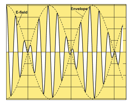
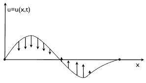
As already mentioned, wave packets can be tailored in time and space to form an optical (pulsed) beam (Sect. 3.1.6). The wave vectors of the Fourier components of such a beam are grouped around a central wave vector $\mathbf{k}^{0}$ that defines the direction of the beam: $\mathbf{k}=\mathbf{k}^{0}+\Delta \mathbf{k}$; each wave vector is related to a frequency $\omega=\omega_{0}+\Delta \omega$ according to the dispersion relation $\omega(\mathbf{k})$ that can be expanded as
$$
\omega(\mathbf{k})=\omega_{0}+\frac{\partial \omega}{\partial \mathbf{k}} \Delta \mathbf{k}+\ldots
$$
The wave packet can be written as three-dimensional integral over $\Delta \mathbf{k}$,
$$
\begin{aligned}
\tilde{\mathbf{E}}(\mathbf{x}, t) &=\int \tilde{\mathbf{E}}(\Delta \mathbf{k}) \mathrm{e}^{-\mathrm{j}\left[\left(\mathbf{k}^{0}+\Delta \mathbf{k}\right) \cdot \mathbf{x}-\omega(\mathbf{k}) t\right]} \mathrm{d}^{3} \Delta \mathbf{k} \
&=\mathrm{e}^{-\mathrm{j}\left(\mathbf{k}^{0} \cdot \mathbf{x}-\omega_{0} t\right)} \int \tilde{\mathbf{E}}(\Delta \mathbf{k}) \mathrm{e}^{-\mathrm{j} \Delta \mathbf{k} \cdot[\mathbf{x}-(\partial \omega / \partial \mathbf{k}) t]} \mathrm{d}^{3} \Delta \mathbf{k},
\end{aligned}
$$
where $\tilde{\mathbf{E}}(\Delta \mathbf{k})$ is the amplitude corresponding to the wave vector $\mathbf{k}^{0}+\Delta \mathbf{k}$. The result is a plane carrier wave $\exp \left[-\mathrm{j}\left(\mathbf{k}^{0} \cdot \mathbf{x}-\omega_{0} t\right)\right]$ with a spatial-temporal envelope represented by the integral; the vectorial group velocity $\mathbf{v}{\text {ray }}$ is obtained by choosing a certain value of the envelope phase $\Delta \mathbf{k} \cdot[\mathbf{x}-(\partial \omega / \partial \mathbf{k}) t]=$ const. and extracting $\dot{\mathbf{x}}$ from the temporal derivative $$ \mathbf{v}{\text {ray }}=\dot{\mathbf{x}}=\left[\begin{array}{l}
\partial \omega / \partial k_{x} \
\partial \omega / \partial k_{y} \
\partial \omega / \partial k_{z}
\end{array}\right]=\nabla_{\mathbf{k}} \omega(\mathbf{k})
$$

电子工程代写|光子简介代写Introduction to Photonics代考|Energy Transport

The energy transport of electromagnetic waves is described by Poynting’s theorem; to derive it, we multiply Eq. (1.13) with $\mathbf{H}$, and (1.14) with $\mathbf{E}$
$$
\mathbf{E} \cdot(\nabla \times \mathbf{H})=\mathbf{E} \cdot \frac{\partial}{\partial t}\left(\varepsilon_{0} \mathbf{E}+\mathbf{P}\right)
$$

$$
\mathbf{H} \cdot(\nabla \times \mathbf{E})=-\mathbf{H} \cdot\left(\mu_{0} \frac{\partial \mathbf{H}}{\partial t}\right)
$$
after subtraction and using $2 \mathbf{a} \cdot(\partial \mathbf{a} / \partial t)=\partial(\mathbf{a} \cdot \mathbf{a}) / \partial t$, we obtain the equation
$$
\mathbf{E} \cdot(\nabla \times \mathbf{H})-\mathbf{H} \cdot(\nabla \times \mathbf{E})=\frac{\partial}{\partial t}\left(\varepsilon_{0} \frac{\mathbf{E} \cdot \mathbf{E}}{2}+\mu_{0} \frac{\mathbf{H} \cdot \mathbf{H}}{2}\right)+\mathbf{E} \cdot \frac{\partial \mathbf{P}}{\partial t}
$$
which, using the identity $\mathbf{b} \cdot(\nabla \times \mathbf{a})-\mathbf{a} \cdot(\nabla \times \mathbf{b})=\nabla \cdot(\mathbf{a} \times \mathbf{b})$, we convert into Poynting’s theorem in its differential form
$$
-\nabla \cdot(\mathbf{E} \times \mathbf{H})=\frac{\partial}{\partial t}\left(\varepsilon_{0} \frac{\mathbf{E} \cdot \mathbf{E}}{2}+\mu_{0} \frac{\mathbf{H} \cdot \mathbf{H}}{2}\right)+\mathbf{E} \cdot \frac{\partial \mathbf{P}}{\partial t}
$$
For the interpretation of the individual terms, we employ the divergence-theorem
$$
\int_{V}(\nabla \cdot \mathbf{u}) \mathrm{d} V=\int_{A} \mathbf{u} \cdot \mathbf{n} \mathrm{d} A
$$
where $A$ is the surface of the volume $V, \mathbf{n}$ is the outward pointing unit normal vector of a surface element, and $\mathrm{d} V, \mathrm{~d} A$ are differential volume and surface elements, respectively, to transform Eq. (1.52) into
$$
\int_{A}[(\mathbf{E} \times \mathbf{H}) \cdot \mathbf{n}] \mathrm{d} A=-\int_{V}\left[\frac{\partial}{\partial t}\left(\varepsilon_{0} \frac{\mathbf{E} \cdot \mathbf{E}}{2}+\mu_{0} \frac{\mathbf{H} \cdot \mathbf{H}}{2}\right)+\mathbf{E} \cdot \frac{\partial \mathbf{P}}{\partial t}\right] \mathrm{d} V .
$$
The terms $\varepsilon_{0} \mathbf{E} \cdot \mathbf{E} / 2$ and $\mu_{0} \mathbf{H} \cdot \mathbf{H} / 2$ represent the electric and magnetic contributions to the vacuum-energy density of the field, while $\mathbf{E} \cdot(\partial \mathbf{P} / \partial t)$ is the power density that is exchanged herween rhe field and rhe medium. Thus, re righr-hand side of Eq. (1.54) is equal to the temporal change of the energy stored in volume $V$. The left-hand side can therefore be interpreted as energy flux through the surface $A$, and the Poynting vector
$$
\mathbf{S}=\mathbf{E} \times \mathbf{H}
$$
as energy flux density [W $\mathrm{m}^{-2}$ ] of the electromagnetic field.

电子工程代写|光子简介代写Introduction to Photonics代考|LEO242

光子简介代考

电子工程代写|光子简介代写Introduction to Photonics代考|Beam Velocity

如前所述,波包可以在时间和空间上进行调整以形成光学 (脉冲) 光束(第 $3.1 .6$ 节) 。这种光束的傅立叶分量的 波向量围绕中心波向量分组 $\mathbf{k}^{0}$ 定义光束的方向: $\mathbf{k}=\mathbf{k}^{0}+\Delta \mathbf{k}$; 每个波矢量都与一个频率有关 $\omega=\omega_{0}+\Delta \omega$ 根 据色散关系 $\omega(\mathbf{k})$ 可以扩展为
$$
\omega(\mathbf{k})=\omega_{0}+\frac{\partial \omega}{\partial \mathbf{k}} \Delta \mathbf{k}+\ldots
$$
波包可以写成三維积分 $\Delta \mathbf{k}$ ,
$$
\tilde{\mathbf{E}}(\mathbf{x}, t)=\int \tilde{\mathbf{E}}(\Delta \mathbf{k}) \mathrm{e}^{-\mathrm{j}\left[\left(\mathbf{k}^{0}+\Delta \mathbf{k}\right) \cdot \mathbf{x}-\omega(\mathbf{k}) t\right]} \mathrm{d}^{3} \Delta \mathbf{k} \quad=\mathrm{e}^{-\mathrm{j}\left(\mathbf{k}^{0} \cdot \mathbf{x}-\omega_{0} t\right)} \int \tilde{\mathbf{E}}(\Delta \mathbf{k}) \mathrm{e}^{-\mathrm{j} \Delta \mathbf{k} \cdot[\mathbf{x}-(\partial \omega / \partial \mathbf{k}) t]} \mathrm{d}^{3} \Delta \mathbf{k},
$$
在哪里 $\tilde{\mathbf{E}}(\Delta \mathbf{k})$ 是对应于波矢量的幅度 $\mathbf{k}^{0}+\Delta \mathbf{k}$. 结果是平面载波 $\exp \left[-\mathrm{j}\left(\mathbf{k}^{0} \cdot \mathbf{x}-\omega_{0} t\right)\right]$ 具有由积分表示的时 空包络;矢量群速度vray 通过选择包络相位的某个值来获得 $\Delta \mathbf{k} \cdot[\mathbf{x}-(\partial \omega / \partial \mathbf{k}) t]=$ 常量。并提取 $\dot{\mathbf{x}}$ 从时间导 数
$$
\text { vray }=\dot{\mathbf{x}}=\left[\partial \omega / \partial k_{x} \partial \omega / \partial k_{y} \partial \omega / \partial k_{z}\right]=\nabla_{\mathbf{k}} \omega(\mathbf{k})
$$

电子工程代写|光子简介代写Introduction to Photonics代考|Energy Transport

波印廷定理描述了电磁波的能量传输;为了推导出它,我们将方程式相乘。(1.13) 与 $\mathbf{H}$, 和 (1.14) 与 $\mathbf{E}$
$$
\begin{aligned}
&\mathbf{E} \cdot(\nabla \times \mathbf{H})=\mathbf{E} \cdot \frac{\partial}{\partial t}\left(\varepsilon_{0} \mathbf{E}+\mathbf{P}\right) \
&\mathbf{H} \cdot(\nabla \times \mathbf{E})=-\mathbf{H} \cdot\left(\mu_{0} \frac{\partial \mathbf{H}}{\partial t}\right)
\end{aligned}
$$
减法和使用后 $2 \mathbf{a} \cdot(\partial \mathbf{a} / \partial t)=\partial(\mathbf{a} \cdot \mathbf{a}) / \partial t$ ,我们得到方程
$$
\mathbf{E} \cdot(\nabla \times \mathbf{H})-\mathbf{H} \cdot(\nabla \times \mathbf{E})=\frac{\partial}{\partial t}\left(\varepsilon_{0} \frac{\mathbf{E} \cdot \mathbf{E}}{2}+\mu_{0} \frac{\mathbf{H} \cdot \mathbf{H}}{2}\right)+\mathbf{E} \cdot \frac{\partial \mathbf{P}}{\partial t}
$$
其中,使用身份 $\mathbf{b} \cdot(\nabla \times \mathbf{a})-\mathbf{a} \cdot(\nabla \times \mathbf{b})=\nabla \cdot(\mathbf{a} \times \mathbf{b})$ ,我们转换成坡印廷定理的微分形式
$$
-\nabla \cdot(\mathbf{E} \times \mathbf{H})=\frac{\partial}{\partial t}\left(\varepsilon_{0} \frac{\mathbf{E} \cdot \mathbf{E}}{2}+\mu_{0} \frac{\mathbf{H} \cdot \mathbf{H}}{2}\right)+\mathbf{E} \cdot \frac{\partial \mathbf{P}}{\partial t}
$$
对于单个术语的解释,我们采用散度定理
$$
\int_{V}(\nabla \cdot \mathbf{u}) \mathrm{d} V=\int_{A} \mathbf{u} \cdot \mathbf{n} \mathrm{d} A
$$
在哪里 $A$ 是体积的表面 $V, \mathbf{n}$ 是表面元素的向外指向单位法向量,并且 $\mathrm{d} V, \mathrm{~d} A$ 分别是微分体积和表面元素,以变 换方程。(1.52) 成
$$
\int_{A}[(\mathbf{E} \times \mathbf{H}) \cdot \mathbf{n}] \mathrm{d} A=-\int_{V}\left[\frac{\partial}{\partial t}\left(\varepsilon_{0} \frac{\mathbf{E} \cdot \mathbf{E}}{2}+\mu_{0} \frac{\mathbf{H} \cdot \mathbf{H}}{2}\right)+\mathbf{E} \cdot \frac{\partial \mathbf{P}}{\partial t}\right] \mathrm{d} V .
$$
条款 $\varepsilon_{0} \mathbf{E} \cdot \mathbf{E} / 2$ 和 $\mu_{0} \mathbf{H} \cdot \mathbf{H} / 2$ 表示电场和磁场对场的真空能量密度的贡献,而 $\mathbf{E} \cdot(\partial \mathbf{P} / \partial t)$ 是在场和介质之间交 换的功率密度。因此,等式的右手边。(1.54) 等于存储在体积中的能量的时间变化 $V$. 因此,左侧可以解释为通过 表面的能量通量 $A$ ,和坡印廷向量
$$
\mathbf{S}=\mathbf{E} \times \mathbf{H}
$$
作为能量通量密度 $\left[\mathrm{Wm}^{-2}\right]$ 的电磁场。

电子工程代写|光子简介代写Introduction to Photonics代考 请认准statistics-lab™

统计代写请认准statistics-lab™. statistics-lab™为您的留学生涯保驾护航。统计代写|python代写代考

随机过程代考

在概率论概念中,随机过程随机变量的集合。 若一随机系统的样本点是随机函数,则称此函数为样本函数,这一随机系统全部样本函数的集合是一个随机过程。 实际应用中,样本函数的一般定义在时间域或者空间域。 随机过程的实例如股票和汇率的波动、语音信号、视频信号、体温的变化,随机运动如布朗运动、随机徘徊等等。

贝叶斯方法代考

贝叶斯统计概念及数据分析表示使用概率陈述回答有关未知参数的研究问题以及统计范式。后验分布包括关于参数的先验分布,和基于观测数据提供关于参数的信息似然模型。根据选择的先验分布和似然模型,后验分布可以解析或近似,例如,马尔科夫链蒙特卡罗 (MCMC) 方法之一。贝叶斯统计概念及数据分析使用后验分布来形成模型参数的各种摘要,包括点估计,如后验平均值、中位数、百分位数和称为可信区间的区间估计。此外,所有关于模型参数的统计检验都可以表示为基于估计后验分布的概率报表。

广义线性模型代考

广义线性模型(GLM)归属统计学领域,是一种应用灵活的线性回归模型。该模型允许因变量的偏差分布有除了正态分布之外的其它分布。

statistics-lab作为专业的留学生服务机构,多年来已为美国、英国、加拿大、澳洲等留学热门地的学生提供专业的学术服务,包括但不限于Essay代写,Assignment代写,Dissertation代写,Report代写,小组作业代写,Proposal代写,Paper代写,Presentation代写,计算机作业代写,论文修改和润色,网课代做,exam代考等等。写作范围涵盖高中,本科,研究生等海外留学全阶段,辐射金融,经济学,会计学,审计学,管理学等全球99%专业科目。写作团队既有专业英语母语作者,也有海外名校硕博留学生,每位写作老师都拥有过硬的语言能力,专业的学科背景和学术写作经验。我们承诺100%原创,100%专业,100%准时,100%满意。

机器学习代写

随着AI的大潮到来,Machine Learning逐渐成为一个新的学习热点。同时与传统CS相比,Machine Learning在其他领域也有着广泛的应用,因此这门学科成为不仅折磨CS专业同学的“小恶魔”,也是折磨生物、化学、统计等其他学科留学生的“大魔王”。学习Machine learning的一大绊脚石在于使用语言众多,跨学科范围广,所以学习起来尤其困难。但是不管你在学习Machine Learning时遇到任何难题,StudyGate专业导师团队都能为你轻松解决。

多元统计分析代考


基础数据: $N$ 个样本, $P$ 个变量数的单样本,组成的横列的数据表
变量定性: 分类和顺序;变量定量:数值
数学公式的角度分为: 因变量与自变量

时间序列分析代写

随机过程,是依赖于参数的一组随机变量的全体,参数通常是时间。 随机变量是随机现象的数量表现,其时间序列是一组按照时间发生先后顺序进行排列的数据点序列。通常一组时间序列的时间间隔为一恒定值(如1秒,5分钟,12小时,7天,1年),因此时间序列可以作为离散时间数据进行分析处理。研究时间序列数据的意义在于现实中,往往需要研究某个事物其随时间发展变化的规律。这就需要通过研究该事物过去发展的历史记录,以得到其自身发展的规律。

回归分析代写

多元回归分析渐进(Multiple Regression Analysis Asymptotics)属于计量经济学领域,主要是一种数学上的统计分析方法,可以分析复杂情况下各影响因素的数学关系,在自然科学、社会和经济学等多个领域内应用广泛。

MATLAB代写

MATLAB 是一种用于技术计算的高性能语言。它将计算、可视化和编程集成在一个易于使用的环境中,其中问题和解决方案以熟悉的数学符号表示。典型用途包括:数学和计算算法开发建模、仿真和原型制作数据分析、探索和可视化科学和工程图形应用程序开发,包括图形用户界面构建MATLAB 是一个交互式系统,其基本数据元素是一个不需要维度的数组。这使您可以解决许多技术计算问题,尤其是那些具有矩阵和向量公式的问题,而只需用 C 或 Fortran 等标量非交互式语言编写程序所需的时间的一小部分。MATLAB 名称代表矩阵实验室。MATLAB 最初的编写目的是提供对由 LINPACK 和 EISPACK 项目开发的矩阵软件的轻松访问,这两个项目共同代表了矩阵计算软件的最新技术。MATLAB 经过多年的发展,得到了许多用户的投入。在大学环境中,它是数学、工程和科学入门和高级课程的标准教学工具。在工业领域,MATLAB 是高效研究、开发和分析的首选工具。MATLAB 具有一系列称为工具箱的特定于应用程序的解决方案。对于大多数 MATLAB 用户来说非常重要,工具箱允许您学习应用专业技术。工具箱是 MATLAB 函数(M 文件)的综合集合,可扩展 MATLAB 环境以解决特定类别的问题。可用工具箱的领域包括信号处理、控制系统、神经网络、模糊逻辑、小波、仿真等。

R语言代写问卷设计与分析代写
PYTHON代写回归分析与线性模型代写
MATLAB代写方差分析与试验设计代写
STATA代写机器学习/统计学习代写
SPSS代写计量经济学代写
EVIEWS代写时间序列分析代写
EXCEL代写深度学习代写
SQL代写各种数据建模与可视化代写

电子工程代写|光子简介代写Introduction to Photonics代考|PHYS3112

如果你也在 怎样代写光子简介Introduction to Photonics这个学科遇到相关的难题,请随时右上角联系我们的24/7代写客服。

光子由一系列的电磁波组成,具有粒子行为。光子学涉及正确使用光作为工具,以造福人类。它源于词根 “光子”,它意味着最微小的光的实体,类似于电力中的电子。

statistics-lab™ 为您的留学生涯保驾护航 在代写光子简介Introduction to Photonics方面已经树立了自己的口碑, 保证靠谱, 高质且原创的统计Statistics代写服务。我们的专家在代写光子简介Introduction to Photonics方面经验极为丰富,各种代写光子简介Introduction to Photonics相关的作业也就用不着说。

我们提供的光子简介Introduction to Photonics及其相关学科的代写,服务范围广, 其中包括但不限于:

  • Statistical Inference 统计推断
  • Statistical Computing 统计计算
  • Advanced Probability Theory 高等楖率论
  • Advanced Mathematical Statistics 高等数理统计学
  • (Generalized) Linear Models 广义线性模型
  • Statistical Machine Learning 统计机器学习
  • Longitudinal Data Analysis 纵向数据分析
  • Foundations of Data Science 数据科学基础
电子工程代写|光子简介代写Introduction to Photonics代考|PHYS3112

电子工程代写|光子简介代写Introduction to Photonics代考|Phase Velocity

To determine the phase velocity of the wave function Eq. (1.26), we choose a certain value of the phase
$$
\mathbf{k} \cdot \mathbf{x}-\omega t=\text { const., }
$$
and calculate the speed at which it propagates through space by taking the spatial derivative
$$
\mathbf{k} \cdot \frac{\mathrm{d} \mathbf{x}}{\mathrm{d} t}-\omega=0 .
$$
The phase velocity in the direction of the wave vector is then, using Eq. (1.28),
$$
v_{\mathrm{ph}}=\left|\frac{\mathrm{d} \mathbf{x}}{\mathrm{d} t}\right|=\frac{\omega}{k}=\frac{c_{0}}{n} .
$$
In vacuum, $n=\sqrt{\varepsilon}=1$ and the phase velocity is equal to the vacuum velocity of light, $c_{0}$. In the visible, this is also a good approximation for the phase velocity in gasses at moderate pressure; the propagation index of transparent condensed media ranges between 1 and about 3 , the corresponding phase velocity between $c_{0}$ and $c_{0} / 3$. The phase velocity is the relevant velocity for the description of interference effects (Chap. 4). The propagation of optical pulses is governed by the so-called group velocity, which we discuss in the following.

电子工程代写|光子简介代写Introduction to Photonics代考|Group Velocity

According to the Fourier theorem, wave packets can be understood as superpositions of monochromatic waves. Since the permittivity $\varepsilon$ and thus the phase velocity of the individual Fourier components is frequency dependent, the propagation velocity of the wave packet may be difficult to define and evaluate. We will treat this problem in some detail in Sect. 3.2. As a first approach, we superimpose two waves with slightly different frequencies and determine the propagation velocity of the resulting “beating” envelope. The two frequencies $\omega_{0} \pm \Delta \omega$ correspond to two wave numbers $k^{0} \pm \Delta k$; assuming equal amplitudes of the two waves, the total field is given by
$$
\begin{aligned}
\mathbf{E}(z, t) &=\operatorname{Re}\left[\mathbf{E}{0} \mathrm{e}^{-\mathrm{j}\left[\left(k^{0}+\Delta k\right) z-\left(\omega{0}+\Delta \omega\right) t\right]}+\mathbf{E}{0} \mathrm{e}^{-\mathrm{j}\left[\left(k^{0}-\Delta k\right) z-\left(\omega{0}-\Delta \omega\right) t\right]}\right] \
&=2 \mathbf{E}{0} \cos (z \Delta k-t \Delta \omega) \cos \left(\omega{0} t-k^{0} z\right)
\end{aligned}
$$
which is an amplitude modulated wave with the carrier frequency $\omega_{0}$ and the envelope $\cos (z \Delta k-t \Delta \omega)$ (Fig.1.2). The envelope propagates at the velocity $\mathrm{d} z / \mathrm{d} t=\Delta \omega / \Delta k$, while the phase fronts move at the phase velocity of the carrier,

$v_{\mathrm{ph}}=\omega_{0} / k^{0}$. For $\Delta \omega \rightarrow 0$, the Taylor expansion
$$
\Delta \omega=\frac{\mathrm{d} \omega}{\mathrm{d} k} \Delta k+\ldots,
$$
allows us to identify $\Delta \omega / \Delta k$ with $\mathrm{d} \omega / \mathrm{d} k$, so that the group velocity can be defined as
$$
v_{\mathrm{g}}:=\frac{\mathrm{d} \omega}{\mathrm{d} k} .
$$

电子工程代写|光子简介代写Introduction to Photonics代考|PHYS3112

光子简介代考

电子工程代写|光子简介代写Introduction to Photonics代考|Phase Velocity

确定波函数方程的相速度。(1.26),我们选择某个相位值
$$
\mathbf{k} \cdot \mathbf{x}-\omega t=\text { const., }
$$
并通过取空间导数计算它在空间中传播的速度
$$
\mathbf{k} \cdot \frac{\mathrm{d} \mathbf{x}}{\mathrm{d} t}-\omega=0
$$
波矢量方向上的相速度然后使用方程。(1.28),
$$
v_{\mathrm{ph}}=\left|\frac{\mathrm{d} \mathbf{x}}{\mathrm{d} t}\right|=\frac{\omega}{k}=\frac{c_{0}}{n} .
$$
在真空中, $n=\sqrt{\varepsilon}=1$ 相速度等于光的真空速度, $c_{0}$. 在可见光中,这也是中等压力下气体相速度的一个很好的 近似值;透明凝聚介质的传播指数介于 1 和 3 之间,对应的相速度介于 $c_{0}$ 和 $c_{0} / 3$. 相速度是描述干涉效应的相关速 度 (第 4 章) 。光脉冲的传播受所谓的群速度控制,我们将在下面讨论。

电子工程代写|光子简介代写Introduction to Photonics代考|Group Velocity

根据傅里叶定理,波包可以理解为单色波的品加。由于介电常数 $\varepsilon$ 因此,各个傅立叶分量的相速度与频率有关,波 包的传播速度可能难以定义和评估。我们将在 Sect 中详细讨论这个问题。3.2. 作为第一种方法,我们唯加两个频 率略有不同的波,并确定产生的“跳动”包络的传播速度。两个频率 $\omega_{0} \pm \Delta \omega$ 对应两个波数 $k^{0} \pm \Delta k$; 假设两个波 的振幅相等,总场由下式给出
$$
\mathbf{E}(z, t)=\operatorname{Re}\left[\mathbf{E} 0 \mathrm{e}^{-\mathrm{j}\left[\left(k^{0}+\Delta k\right) z-(\omega 0+\Delta \omega) t\right]}+\mathbf{E} 0 \mathrm{e}^{-\mathrm{j}\left[\left(k^{0}-\Delta k\right) z-(\omega 0-\Delta \omega) t\right]}\right] \quad=2 \mathbf{E} 0 \cos (z \Delta k-t \Delta \omega) \cos
$$
它是一个带有载波频率的调幅波 $\omega_{0}$ 和信封 $\cos (z \Delta k-t \Delta \omega$ )(图 1.2)。包络以速度传播 $\mathrm{d} z / \mathrm{d} t=\Delta \omega / \Delta k$ , 而相位前沿以载波的相速度移动,
$v_{\mathrm{ph}}=\omega_{0} / k^{0}$. 为了 $\Delta \omega \rightarrow 0$, 泰勒展开
$$
\Delta \omega=\frac{\mathrm{d} \omega}{\mathrm{d} k} \Delta k+\ldots,
$$
允许我们识别 $\Delta \omega / \Delta k$ 和 $\mathrm{d} \omega / \mathrm{d} k$ ,因此群速度可以定义为
$$
v_{\mathrm{g}}:=\frac{\mathrm{d} \omega}{\mathrm{d} k} .
$$

电子工程代写|光子简介代写Introduction to Photonics代考 请认准statistics-lab™

统计代写请认准statistics-lab™. statistics-lab™为您的留学生涯保驾护航。统计代写|python代写代考

随机过程代考

在概率论概念中,随机过程随机变量的集合。 若一随机系统的样本点是随机函数,则称此函数为样本函数,这一随机系统全部样本函数的集合是一个随机过程。 实际应用中,样本函数的一般定义在时间域或者空间域。 随机过程的实例如股票和汇率的波动、语音信号、视频信号、体温的变化,随机运动如布朗运动、随机徘徊等等。

贝叶斯方法代考

贝叶斯统计概念及数据分析表示使用概率陈述回答有关未知参数的研究问题以及统计范式。后验分布包括关于参数的先验分布,和基于观测数据提供关于参数的信息似然模型。根据选择的先验分布和似然模型,后验分布可以解析或近似,例如,马尔科夫链蒙特卡罗 (MCMC) 方法之一。贝叶斯统计概念及数据分析使用后验分布来形成模型参数的各种摘要,包括点估计,如后验平均值、中位数、百分位数和称为可信区间的区间估计。此外,所有关于模型参数的统计检验都可以表示为基于估计后验分布的概率报表。

广义线性模型代考

广义线性模型(GLM)归属统计学领域,是一种应用灵活的线性回归模型。该模型允许因变量的偏差分布有除了正态分布之外的其它分布。

statistics-lab作为专业的留学生服务机构,多年来已为美国、英国、加拿大、澳洲等留学热门地的学生提供专业的学术服务,包括但不限于Essay代写,Assignment代写,Dissertation代写,Report代写,小组作业代写,Proposal代写,Paper代写,Presentation代写,计算机作业代写,论文修改和润色,网课代做,exam代考等等。写作范围涵盖高中,本科,研究生等海外留学全阶段,辐射金融,经济学,会计学,审计学,管理学等全球99%专业科目。写作团队既有专业英语母语作者,也有海外名校硕博留学生,每位写作老师都拥有过硬的语言能力,专业的学科背景和学术写作经验。我们承诺100%原创,100%专业,100%准时,100%满意。

机器学习代写

随着AI的大潮到来,Machine Learning逐渐成为一个新的学习热点。同时与传统CS相比,Machine Learning在其他领域也有着广泛的应用,因此这门学科成为不仅折磨CS专业同学的“小恶魔”,也是折磨生物、化学、统计等其他学科留学生的“大魔王”。学习Machine learning的一大绊脚石在于使用语言众多,跨学科范围广,所以学习起来尤其困难。但是不管你在学习Machine Learning时遇到任何难题,StudyGate专业导师团队都能为你轻松解决。

多元统计分析代考


基础数据: $N$ 个样本, $P$ 个变量数的单样本,组成的横列的数据表
变量定性: 分类和顺序;变量定量:数值
数学公式的角度分为: 因变量与自变量

时间序列分析代写

随机过程,是依赖于参数的一组随机变量的全体,参数通常是时间。 随机变量是随机现象的数量表现,其时间序列是一组按照时间发生先后顺序进行排列的数据点序列。通常一组时间序列的时间间隔为一恒定值(如1秒,5分钟,12小时,7天,1年),因此时间序列可以作为离散时间数据进行分析处理。研究时间序列数据的意义在于现实中,往往需要研究某个事物其随时间发展变化的规律。这就需要通过研究该事物过去发展的历史记录,以得到其自身发展的规律。

回归分析代写

多元回归分析渐进(Multiple Regression Analysis Asymptotics)属于计量经济学领域,主要是一种数学上的统计分析方法,可以分析复杂情况下各影响因素的数学关系,在自然科学、社会和经济学等多个领域内应用广泛。

MATLAB代写

MATLAB 是一种用于技术计算的高性能语言。它将计算、可视化和编程集成在一个易于使用的环境中,其中问题和解决方案以熟悉的数学符号表示。典型用途包括:数学和计算算法开发建模、仿真和原型制作数据分析、探索和可视化科学和工程图形应用程序开发,包括图形用户界面构建MATLAB 是一个交互式系统,其基本数据元素是一个不需要维度的数组。这使您可以解决许多技术计算问题,尤其是那些具有矩阵和向量公式的问题,而只需用 C 或 Fortran 等标量非交互式语言编写程序所需的时间的一小部分。MATLAB 名称代表矩阵实验室。MATLAB 最初的编写目的是提供对由 LINPACK 和 EISPACK 项目开发的矩阵软件的轻松访问,这两个项目共同代表了矩阵计算软件的最新技术。MATLAB 经过多年的发展,得到了许多用户的投入。在大学环境中,它是数学、工程和科学入门和高级课程的标准教学工具。在工业领域,MATLAB 是高效研究、开发和分析的首选工具。MATLAB 具有一系列称为工具箱的特定于应用程序的解决方案。对于大多数 MATLAB 用户来说非常重要,工具箱允许您学习应用专业技术。工具箱是 MATLAB 函数(M 文件)的综合集合,可扩展 MATLAB 环境以解决特定类别的问题。可用工具箱的领域包括信号处理、控制系统、神经网络、模糊逻辑、小波、仿真等。

R语言代写问卷设计与分析代写
PYTHON代写回归分析与线性模型代写
MATLAB代写方差分析与试验设计代写
STATA代写机器学习/统计学习代写
SPSS代写计量经济学代写
EVIEWS代写时间序列分析代写
EXCEL代写深度学习代写
SQL代写各种数据建模与可视化代写

电子工程代写|光子简介代写Introduction to Photonics代考|ELEC3405

如果你也在 怎样代写光子简介Introduction to Photonics这个学科遇到相关的难题,请随时右上角联系我们的24/7代写客服。

光子由一系列的电磁波组成,具有粒子行为。光子学涉及正确使用光作为工具,以造福人类。它源于词根 “光子”,它意味着最微小的光的实体,类似于电力中的电子。

statistics-lab™ 为您的留学生涯保驾护航 在代写光子简介Introduction to Photonics方面已经树立了自己的口碑, 保证靠谱, 高质且原创的统计Statistics代写服务。我们的专家在代写光子简介Introduction to Photonics方面经验极为丰富,各种代写光子简介Introduction to Photonics相关的作业也就用不着说。

我们提供的光子简介Introduction to Photonics及其相关学科的代写,服务范围广, 其中包括但不限于:

  • Statistical Inference 统计推断
  • Statistical Computing 统计计算
  • Advanced Probability Theory 高等楖率论
  • Advanced Mathematical Statistics 高等数理统计学
  • (Generalized) Linear Models 广义线性模型
  • Statistical Machine Learning 统计机器学习
  • Longitudinal Data Analysis 纵向数据分析
  • Foundations of Data Science 数据科学基础
电子工程代写|光子简介代写Introduction to Photonics代考|ELEC3405

电子工程代写|光子简介代写Introduction to Photonics代考|Complex Wave Functions and Amplitudes

The structure of Eq. (1.20) allows us to factorize its solutions $\mathbf{E}(\mathbf{x}, t)$ into a spatial and a temporal part. For the temporal part, we choose harmonically oscillating functions: not only do they describe the output of a single mode laser very well, they also represent the base for the Fourier decomposition of more general time varying signals. The ansatz
$$
\mathbf{E}(\mathbf{x}, t)=\operatorname{Re}\left[\tilde{\mathbf{E}}(\mathbf{x}, \omega) \mathrm{e}^{\mathrm{j} \omega t}\right]=\frac{1}{2}\left[\tilde{\mathbf{E}}(\mathbf{x}, \omega) \mathrm{e}^{\mathrm{j} \omega t}+c . c .\right]
$$
where $\omega$ is the angular frequency and c.c. stands for “complex conjugate,” is a solution of Eq. (1.20), if $\tilde{\mathbf{E}}(\mathbf{x}, \omega)$ is a solution of the Helmholtz equation
$$
\nabla^{2} \tilde{\mathbf{E}}(\mathbf{x}, \omega)+\frac{\omega^{2} \varepsilon}{c_{0}^{2}} \tilde{\mathbf{E}}(\mathbf{x}, \omega)=\mathbf{0}
$$
In cartesian coordinates, each component of $\tilde{E}{i}$ must be a solution of the scalar Helmholtz equation $$ \left[\frac{\partial^{2}}{\partial x^{2}}+\frac{\partial^{2}}{\partial y^{2}}+\frac{\partial^{2}}{\partial z^{2}}+\frac{\omega^{2} \varepsilon}{c{0}^{2}}\right] \tilde{E}_{i}(\mathbf{x}, \omega)=0
$$
A particularly simple solution is the harmonically oscillating function
$$
\tilde{\mathbf{E}}(\mathbf{x}, \omega)=\tilde{\mathbf{E}}(\mathbf{k}, \omega) \mathrm{e}^{-\mathrm{j} \mathbf{k} \cdot \mathbf{x}}
$$
where $\mathbf{k}$ is known as wave vector and its absolute value $k$ as angular wave number ${ }^{2}$ or propagation constant. The complete electric wave function is then
$$
\mathbf{E}(\mathbf{x}, t)=\operatorname{Re}[\tilde{\mathbf{E}}(\mathbf{x}, t)],
$$
where
$$
\tilde{\mathbf{E}}(\mathbf{x}, t)=\overline{\mathbf{E}}(\mathbf{k}, \omega) \mathrm{e}^{-J(\mathbf{k} \cdot \mathbf{x}-\omega t)}
$$
is the so-called complex wave function and $\tilde{\mathbf{E}}(\mathbf{k}, \omega)$ the complex amplitude; the imaginary part of the argument of the exponential function is called phase. Inserting Eq. (1.26) into the Helmholtz equation Eq.

电子工程代写|光子简介代写Introduction to Photonics代考|Plane Waves

Surfaces of constant phase of Eq. (1.26), $\mathbf{k} \cdot \mathbf{x}-\omega t=$ const., are planes normal to the wave vector $\mathbf{k}$ (Fig. 1.1); these waves therefore are called plane waves; the distance between planes of equal phase are separated by integer multiples of the so-called wavelength
$$
\lambda:=\frac{2 \pi}{|\mathbf{k}|} .
$$
The number $k / 2 \pi$ is equal to the number of spatial periods per unit length, measured in the direction of $\mathbf{k} ; k$ is therefore also called spatial (angular) frequency. In vacuum,
$$
\lambda_{0}=\frac{2 \pi}{k_{0}}=2 \pi \frac{c_{0}}{\omega} ;
$$
the vacuum wavelength in the optical region of the electromagnetic spectrum is of the order of $1 \mu \mathrm{m}$. The corresponding temporal oscillation period, $2 \pi / \omega$, is about $3 \times 10^{-15} \mathrm{~s}$, or 3 femtoseconds (fs).

Similar to harmonically oscillating temporal functions that allow “synthesizing” arbitrary temporal functions, plane waves can be used to synthesize arbitrary spatial wave functions via a Fourier integral over all possible wave vectors (Sect. 3.1.6).
In practice, there are different conventions to specify the frequency of a wave: the temporal frequency $\nu=\omega / 2 \pi$, the quantum energy $\hbar \omega$, the spatial vacuum frequency (spectroscopic wave number) $k / 2 \pi=1 / \lambda_{0}$, or the vacuum wave length $\lambda_{0}$. Table $1.1$ summarizes the relations between the different parameters.

电子工程代写|光子简介代写Introduction to Photonics代考|ELEC3405

光子简介代考

电子工程代写|光子简介代写Introduction to Photonics代考|Complex Wave Functions and Amplitudes

方程式的结构。(1.20) 允许我们分解它的解决方案 $\mathbf{E}(\mathbf{x}, t)$ 分为空间部分和时间部分。对于时间部分,我们选择 谐波振荡函数:它们不仅很好地描述了单模激光器的输出,还代表了更一般的时变信号的傅里叶分解的基础。安萨 茨
$$
\mathbf{E}(\mathbf{x}, t)=\operatorname{Re}\left[\tilde{\mathbf{E}}(\mathbf{x}, \omega) \mathrm{e}^{\mathrm{j} \omega t}\right]=\frac{1}{2}\left[\tilde{\mathbf{E}}(\mathbf{x}, \omega) \mathrm{e}^{\mathrm{j} \omega t}+c . c .\right]
$$
在哪里 $\omega$ 是角频率, $c \mathrm{C}$ 代表”复共轭”,是等式的解。(1.20),如果 $\tilde{\mathbf{E}}(\mathbf{x}, \omega)$ 是亥姆霍兹方程的解
$$
\nabla^{2} \tilde{\mathbf{E}}(\mathbf{x}, \omega)+\frac{\omega^{2} \varepsilon}{c_{0}^{2}} \tilde{\mathbf{E}}(\mathbf{x}, \omega)=\mathbf{0}
$$
在笛卡尔坐标中,每个分量 $\tilde{E} i$ 必须是标量亥姆霍兹方程的解
$$
\left[\frac{\partial^{2}}{\partial x^{2}}+\frac{\partial^{2}}{\partial y^{2}}+\frac{\partial^{2}}{\partial z^{2}}+\frac{\omega^{2} \varepsilon}{c 0^{2}}\right] \tilde{E}_{i}(\mathbf{x}, \omega)=0
$$
一个特别简单的解决方案是谐波振荡函数
$$
\tilde{\mathbf{E}}(\mathbf{x}, \omega)=\tilde{\mathbf{E}}(\mathbf{k}, \omega) \mathrm{e}^{-\mathrm{j} \mathbf{k} \cdot \mathbf{x}}
$$
在哪里 $\mathbf{k}$ 被称为波矢量及其绝对值 $k$ 作为角波数 ${ }^{2}$ 或传播常数。则完整的电波函数为
$$
\mathbf{E}(\mathbf{x}, t)=\operatorname{Re}[\tilde{\mathbf{E}}(\mathbf{x}, t)],
$$
在哪里
$$
\tilde{\mathbf{E}}(\mathbf{x}, t)=\overline{\mathbf{E}}(\mathbf{k}, \omega) \mathrm{e}^{-J(\mathbf{k} \cdot \mathbf{x}-\omega t)}
$$
是所谓的复波函数和 $\tilde{\mathbf{E}}(\mathbf{k}, \omega)$ 复振幅;指数函数的自变量的虚部称为相位。揷入方程式。(1.26) 进入亥姆霍兹方程方程。

电子工程代写|光子简介代写Introduction to Photonics代考|Plane Waves

等式的恒定相位表面。(1.26), $\mathbf{k} \cdot \mathbf{x}-\omega t=$ const., 是垂直于波矢量的平面 $\mathbf{k}$ (图 1.1);因此,这些波被称为平面 波;等相位平面之间的距离被所谓波长的整数倍分开
$$
\lambda:=\frac{2 \pi}{|\mathbf{k}|} .
$$
号码 $k / 2 \pi$ 等于每单位长度的空间周期数,在方向上测量 $\mathbf{k} ; k$ 因此也称为空间(角)频率。在真空中,
$$
\lambda_{0}=\frac{2 \pi}{k_{0}}=2 \pi \frac{c_{0}}{\omega} ;
$$
电磁光谱的光学区域中的真空波长约为 $1 \mu \mathrm{m}$. 相应的时间振萡周期, $2 \pi / \omega$ ,约是 $3 \times 10^{-15} \mathrm{~s}$ ,或 $3 飞$ 秒 (fs)。
与允许“合成”任意时间函数的诣波振荡时间函数类似,平面波可用于通过对所有可能的波向量进行傅里叶积分来合 成任意空间波函数(第 $3.1 .6$ 节)。
在实践中,有不同的约定来指定波的频率:时间频率 $\nu=\omega / 2 \pi$ ,量子能量 $\hbar \omega$ ,空间真空频率 (光谱波数) $k / 2 \pi=1 / \lambda_{0}$ ,或真空波长 $\lambda_{0}$. 桌子 $1.1$ 总结了不同参数之间的关系。

电子工程代写|光子简介代写Introduction to Photonics代考 请认准statistics-lab™

统计代写请认准statistics-lab™. statistics-lab™为您的留学生涯保驾护航。统计代写|python代写代考

随机过程代考

在概率论概念中,随机过程随机变量的集合。 若一随机系统的样本点是随机函数,则称此函数为样本函数,这一随机系统全部样本函数的集合是一个随机过程。 实际应用中,样本函数的一般定义在时间域或者空间域。 随机过程的实例如股票和汇率的波动、语音信号、视频信号、体温的变化,随机运动如布朗运动、随机徘徊等等。

贝叶斯方法代考

贝叶斯统计概念及数据分析表示使用概率陈述回答有关未知参数的研究问题以及统计范式。后验分布包括关于参数的先验分布,和基于观测数据提供关于参数的信息似然模型。根据选择的先验分布和似然模型,后验分布可以解析或近似,例如,马尔科夫链蒙特卡罗 (MCMC) 方法之一。贝叶斯统计概念及数据分析使用后验分布来形成模型参数的各种摘要,包括点估计,如后验平均值、中位数、百分位数和称为可信区间的区间估计。此外,所有关于模型参数的统计检验都可以表示为基于估计后验分布的概率报表。

广义线性模型代考

广义线性模型(GLM)归属统计学领域,是一种应用灵活的线性回归模型。该模型允许因变量的偏差分布有除了正态分布之外的其它分布。

statistics-lab作为专业的留学生服务机构,多年来已为美国、英国、加拿大、澳洲等留学热门地的学生提供专业的学术服务,包括但不限于Essay代写,Assignment代写,Dissertation代写,Report代写,小组作业代写,Proposal代写,Paper代写,Presentation代写,计算机作业代写,论文修改和润色,网课代做,exam代考等等。写作范围涵盖高中,本科,研究生等海外留学全阶段,辐射金融,经济学,会计学,审计学,管理学等全球99%专业科目。写作团队既有专业英语母语作者,也有海外名校硕博留学生,每位写作老师都拥有过硬的语言能力,专业的学科背景和学术写作经验。我们承诺100%原创,100%专业,100%准时,100%满意。

机器学习代写

随着AI的大潮到来,Machine Learning逐渐成为一个新的学习热点。同时与传统CS相比,Machine Learning在其他领域也有着广泛的应用,因此这门学科成为不仅折磨CS专业同学的“小恶魔”,也是折磨生物、化学、统计等其他学科留学生的“大魔王”。学习Machine learning的一大绊脚石在于使用语言众多,跨学科范围广,所以学习起来尤其困难。但是不管你在学习Machine Learning时遇到任何难题,StudyGate专业导师团队都能为你轻松解决。

多元统计分析代考


基础数据: $N$ 个样本, $P$ 个变量数的单样本,组成的横列的数据表
变量定性: 分类和顺序;变量定量:数值
数学公式的角度分为: 因变量与自变量

时间序列分析代写

随机过程,是依赖于参数的一组随机变量的全体,参数通常是时间。 随机变量是随机现象的数量表现,其时间序列是一组按照时间发生先后顺序进行排列的数据点序列。通常一组时间序列的时间间隔为一恒定值(如1秒,5分钟,12小时,7天,1年),因此时间序列可以作为离散时间数据进行分析处理。研究时间序列数据的意义在于现实中,往往需要研究某个事物其随时间发展变化的规律。这就需要通过研究该事物过去发展的历史记录,以得到其自身发展的规律。

回归分析代写

多元回归分析渐进(Multiple Regression Analysis Asymptotics)属于计量经济学领域,主要是一种数学上的统计分析方法,可以分析复杂情况下各影响因素的数学关系,在自然科学、社会和经济学等多个领域内应用广泛。

MATLAB代写

MATLAB 是一种用于技术计算的高性能语言。它将计算、可视化和编程集成在一个易于使用的环境中,其中问题和解决方案以熟悉的数学符号表示。典型用途包括:数学和计算算法开发建模、仿真和原型制作数据分析、探索和可视化科学和工程图形应用程序开发,包括图形用户界面构建MATLAB 是一个交互式系统,其基本数据元素是一个不需要维度的数组。这使您可以解决许多技术计算问题,尤其是那些具有矩阵和向量公式的问题,而只需用 C 或 Fortran 等标量非交互式语言编写程序所需的时间的一小部分。MATLAB 名称代表矩阵实验室。MATLAB 最初的编写目的是提供对由 LINPACK 和 EISPACK 项目开发的矩阵软件的轻松访问,这两个项目共同代表了矩阵计算软件的最新技术。MATLAB 经过多年的发展,得到了许多用户的投入。在大学环境中,它是数学、工程和科学入门和高级课程的标准教学工具。在工业领域,MATLAB 是高效研究、开发和分析的首选工具。MATLAB 具有一系列称为工具箱的特定于应用程序的解决方案。对于大多数 MATLAB 用户来说非常重要,工具箱允许您学习应用专业技术。工具箱是 MATLAB 函数(M 文件)的综合集合,可扩展 MATLAB 环境以解决特定类别的问题。可用工具箱的领域包括信号处理、控制系统、神经网络、模糊逻辑、小波、仿真等。

R语言代写问卷设计与分析代写
PYTHON代写回归分析与线性模型代写
MATLAB代写方差分析与试验设计代写
STATA代写机器学习/统计学习代写
SPSS代写计量经济学代写
EVIEWS代写时间序列分析代写
EXCEL代写深度学习代写
SQL代写各种数据建模与可视化代写

电子工程代写|光子简介代写Introduction to Photonics代考|ECSE423

如果你也在 怎样代写光子简介Introduction to Photonics这个学科遇到相关的难题,请随时右上角联系我们的24/7代写客服。

光子由一系列的电磁波组成,具有粒子行为。光子学涉及正确使用光作为工具,以造福人类。它源于词根 “光子”,它意味着最微小的光的实体,类似于电力中的电子。

statistics-lab™ 为您的留学生涯保驾护航 在代写光子简介Introduction to Photonics方面已经树立了自己的口碑, 保证靠谱, 高质且原创的统计Statistics代写服务。我们的专家在代写光子简介Introduction to Photonics方面经验极为丰富,各种代写光子简介Introduction to Photonics相关的作业也就用不着说。

我们提供的光子简介Introduction to Photonics及其相关学科的代写,服务范围广, 其中包括但不限于:

  • Statistical Inference 统计推断
  • Statistical Computing 统计计算
  • Advanced Probability Theory 高等楖率论
  • Advanced Mathematical Statistics 高等数理统计学
  • (Generalized) Linear Models 广义线性模型
  • Statistical Machine Learning 统计机器学习
  • Longitudinal Data Analysis 纵向数据分析
  • Foundations of Data Science 数据科学基础
电子工程代写|光子简介代写Introduction to Photonics代考|ECSE423

电子工程代写|光子简介代写Introduction to Photonics代考|The Electromagnetic Field

Maxwell’s equations, relating the electric field $\mathbf{E}\left[\mathrm{Vm}^{-1}\right]$ and the magnetic field $\mathbf{H}$ $\left[\mathrm{Am}^{-1}\right]$ in a medium with polarization density $\mathbf{P}\left[\mathrm{Asm}^{-2}\right]$, magnetization density $\mathbf{M}\left[\mathrm{Am}^{-1}\right]$, density of free charges $\rho\left[\mathrm{Asm}^{-3}\right]$, and current density $\mathbf{j}\left[\mathrm{Am}^{-2}\right]$, have the form
$$
\begin{aligned}
&\nabla \times \mathbf{E}=-\mu_{0} \frac{\partial \mathbf{H}}{\partial t}-\mu_{0} \frac{\partial \mathbf{M}}{\partial t} \
&\nabla \times \mathbf{H}=\varepsilon_{0} \frac{\partial \mathbf{E}}{\partial t}+\frac{\partial \mathbf{P}}{\partial t}+\mathbf{j}
\end{aligned}
$$

$$
\begin{aligned}
\nabla \cdot\left(\varepsilon_{0} \mathbf{E}\right) &=-\nabla \cdot \mathbf{P}+\rho \
\nabla \cdot\left(\mu_{0} \mathbf{H}\right) &=-\nabla \cdot\left(\mu_{0} \mathbf{M}\right),
\end{aligned}
$$
where $\varepsilon_{0}=8.854 \times 10^{-12} \mathrm{AsV}^{-1} \mathrm{~m}^{-1}$ is the vacuum permittivity and $\mu_{0}=4 \pi 10^{-7} \mathrm{VsA}^{-1} \mathrm{~m}^{-1}$ the magnetic constant (also called vacuum permeability). In cartesian coordinates, the differential operator $\nabla$ is given by
$$
\nabla=\left[\begin{array}{l}
\partial / \partial x \
\partial / \partial y \
\partial / \partial z
\end{array}\right]
$$
or
$$
\nabla=[\partial / \partial x, \partial / \partial y, \partial / \partial z],
$$
depending on the vector operation. $\mathbf{P}$ is the response of the medium to the electric field and, for moderate optical fields, a linear function of $\mathbf{E}$,
$$
\mathbf{P}=\varepsilon_{0} \chi \mathbf{E}
$$
$\chi$ is the (dimensionless) electric susceptibility and represents the dielectric properties of the medium. It is common to introduce the electric displacement density $\mathbf{D}$ $\left[\mathrm{Asm}^{-2}\right]$
$$
\mathbf{D}:=\varepsilon_{0} \mathbf{E}+\mathbf{P}
$$
that combines the “vacuum displacement density” $\varepsilon_{0} \mathbf{E}$ with the material polarization density.

电子工程代写|光子简介代写Introduction to Photonics代考|Wave Equation

We can eliminate the magnetic field from Eqs. (1.13) and (1.14) to obtain a single wave equation for the electric field: taking the rotation of Eq. (1.13) and substituting the time derivative of Eq. (1.14), we obtain
$$
\nabla \times(\nabla \times \mathbf{E})+\mu_{0} \frac{\partial^{2} \mathbf{D}}{\partial t^{2}}=\mathbf{0} .
$$
In isotropic media, the relation between $\mathbf{P}$ and $\mathbf{E}$ is expressed by a scalar susceptibility $\chi$, and $\varepsilon=1+\chi$. From Eq. (1.3) in the form $\nabla \cdot \mathbf{D}=\nabla \cdot \varepsilon \varepsilon_{0} \mathbf{E}=0$ follows, for homogeneous media, $\nabla \cdot \mathbf{E}=0$. With the identity
$$
\nabla \times(\nabla \times \mathbf{a})=\nabla(\nabla \cdot \mathbf{a})-\nabla^{2} \mathbf{a},
$$
we can formulate Eq. (1.15) as
$$
-\nabla^{2} \mathbf{E}+\mu_{0} \frac{\partial^{2} \mathbf{D}}{\partial t^{2}}=\mathbf{0},
$$
where the Laplace operator $\nabla^{2}$, in cartesian coordinates, is given by
$$
\nabla^{2}=\frac{\partial^{2}}{\partial x^{2}}+\frac{\partial^{2}}{\partial y^{2}}+\frac{\partial^{2}}{\partial z^{2}} .
$$
With
$$
c_{0}:=\frac{1}{\sqrt{\varepsilon_{0} \mu_{0}}},
$$
Eq. (1.17) assumes the form
$$
\nabla^{2} \mathbf{E}(\mathbf{x}, t)-\frac{\varepsilon}{c_{0}^{3}} \frac{\partial^{2} \mathbf{E}(\mathbf{x}, t)}{\partial t^{2}}=\mathbf{0} ;
$$
for reasons that will become obvious, $c_{0}=2.998 \times 10^{8} \mathrm{~ms}^{-1}$ is called vacuum speed of light. Equation (1.20) is the wave equation for the electric field in isotropic, linear, and local media.

电子工程代写|光子简介代写Introduction to Photonics代考|ECSE423

光子简介代考

电子工程代写|光子简介代写Introduction to Photonics代考|The Electromagnetic Field

麦克斯韦方程,与电场有关 $\mathbf{E}\left[\mathrm{Vm}^{-1}\right]$ 和磁场 $\mathbf{H}\left[\mathrm{Am}^{-1}\right]$ 在具有极化密度的介质中 $\mathbf{P}\left[\mathrm{Asm}^{-2}\right]$, 磁化密度 $\mathbf{M}\left[\mathrm{Am}^{-1}\right]$, 免费费用的密度 $\rho\left[\mathrm{Asm}^{-3}\right]$, 和电流密度 $\mathbf{j}\left[\mathrm{Am}^{-2}\right]$ ,有形式
$$
\begin{aligned}
\nabla \times \mathbf{E}=-\mu_{0} \frac{\partial \mathbf{H}}{\partial t}-\mu_{0} \frac{\partial \mathbf{M}}{\partial t} \quad \nabla \times \mathbf{H} &=\varepsilon_{0} \frac{\partial \mathbf{E}}{\partial t}+\frac{\partial \mathbf{P}}{\partial t}+\mathbf{j} \
\nabla \cdot\left(\varepsilon_{0} \mathbf{E}\right)=-\nabla \cdot \mathbf{P}+\rho \nabla \cdot\left(\mu_{0} \mathbf{H}\right) &=-\nabla \cdot\left(\mu_{0} \mathbf{M}\right),
\end{aligned}
$$
在哪里 $\varepsilon_{0}=8.854 \times 10^{-12} \mathrm{AsV}^{-1} \mathrm{~m}^{-1}$ 是真空介电常数和 $\mu_{0}=4 \pi 10^{-7} \mathrm{VsA}^{-1} \mathrm{~m}^{-1}$ 磁常数 (也称为真空 磁导率) 。在笛卡尔坐标中,微分算子 $\nabla$ 是 (谁) 给的
$$
\nabla=[\partial / \partial x \partial / \partial y \partial / \partial z]
$$
或者
$$
\nabla=[\partial / \partial x, \partial / \partial y, \partial / \partial z]
$$
取决于向量运算。 $\mathbf{P}$ 是介质对电场的响应,对于中等光场,它是一个线性函数 $\mathbf{E}$ ,
$$
\mathbf{P}=\varepsilon_{0} \chi \mathbf{E}
$$
$\chi$ 是 (无量纲的) 电敏感性,代表介质的介电特性。通常引入电位移密度 $\mathbf{D}\left[\mathrm{Asm}^{-2}\right]$
$$
\mathbf{D}:=\varepsilon_{0} \mathbf{E}+\mathbf{P}
$$
结合了”真空位移密度” $\varepsilon_{0} \mathbf{E}$ 与材料极化密度。

电子工程代写|光子简介代写Introduction to Photonics代考|Wave Equation

我们可以从方程式中消除磁场。(1.13) 和 (1.14) 得到电场的单波动方程:取方程的旋转。(1.13) 并代入方程 式的时间导数。(1.14),我们得到
$$
\nabla \times(\nabla \times \mathbf{E})+\mu_{0} \frac{\partial^{2} \mathbf{D}}{\partial t^{2}}=\mathbf{0} .
$$
在各向同性介质中,之间的关系 $\mathbf{P}$ 和 $\mathbf{E}$ 用标量磁化率表示 $\chi$ ,和 $\varepsilon=1+\chi$. 从方程式。(1.3) 形式 $\nabla \cdot \mathbf{D}=\nabla \cdot \varepsilon \varepsilon_{0} \mathbf{E}=0$ 接下来,对于同质介质, $\nabla \cdot \mathbf{E}=0$. 带着身份
$$
\nabla \times(\nabla \times \mathbf{a})=\nabla(\nabla \cdot \mathbf{a})-\nabla^{2} \mathbf{a},
$$
我们可以制定方程式。(1.15) 为
$$
-\nabla^{2} \mathbf{E}+\mu_{0} \frac{\partial^{2} \mathbf{D}}{\partial t^{2}}=\mathbf{0}
$$
拉普拉斯算子在哪里 $\nabla^{2}$ ,在笛卡尔坐标中,由下式给出
$$
\nabla^{2}=\frac{\partial^{2}}{\partial x^{2}}+\frac{\partial^{2}}{\partial y^{2}}+\frac{\partial^{2}}{\partial z^{2}} .
$$

$$
c_{0}:=\frac{1}{\sqrt{\varepsilon_{0} \mu_{0}}}
$$
方程。(1.17) 采用形式
$$
\nabla^{2} \mathbf{E}(\mathbf{x}, t)-\frac{\varepsilon}{c_{0}^{3}} \frac{\partial^{2} \mathbf{E}(\mathbf{x}, t)}{\partial t^{2}}=\mathbf{0}
$$
出于显而易见的原因, $c_{0}=2.998 \times 10^{8} \mathrm{~ms}^{-1}$ 称为真空光速。方程 $(1.20)$ 是各向同性、线性和局部介质中电场 的波动方程。

电子工程代写|光子简介代写Introduction to Photonics代考 请认准statistics-lab™

统计代写请认准statistics-lab™. statistics-lab™为您的留学生涯保驾护航。统计代写|python代写代考

随机过程代考

在概率论概念中,随机过程随机变量的集合。 若一随机系统的样本点是随机函数,则称此函数为样本函数,这一随机系统全部样本函数的集合是一个随机过程。 实际应用中,样本函数的一般定义在时间域或者空间域。 随机过程的实例如股票和汇率的波动、语音信号、视频信号、体温的变化,随机运动如布朗运动、随机徘徊等等。

贝叶斯方法代考

贝叶斯统计概念及数据分析表示使用概率陈述回答有关未知参数的研究问题以及统计范式。后验分布包括关于参数的先验分布,和基于观测数据提供关于参数的信息似然模型。根据选择的先验分布和似然模型,后验分布可以解析或近似,例如,马尔科夫链蒙特卡罗 (MCMC) 方法之一。贝叶斯统计概念及数据分析使用后验分布来形成模型参数的各种摘要,包括点估计,如后验平均值、中位数、百分位数和称为可信区间的区间估计。此外,所有关于模型参数的统计检验都可以表示为基于估计后验分布的概率报表。

广义线性模型代考

广义线性模型(GLM)归属统计学领域,是一种应用灵活的线性回归模型。该模型允许因变量的偏差分布有除了正态分布之外的其它分布。

statistics-lab作为专业的留学生服务机构,多年来已为美国、英国、加拿大、澳洲等留学热门地的学生提供专业的学术服务,包括但不限于Essay代写,Assignment代写,Dissertation代写,Report代写,小组作业代写,Proposal代写,Paper代写,Presentation代写,计算机作业代写,论文修改和润色,网课代做,exam代考等等。写作范围涵盖高中,本科,研究生等海外留学全阶段,辐射金融,经济学,会计学,审计学,管理学等全球99%专业科目。写作团队既有专业英语母语作者,也有海外名校硕博留学生,每位写作老师都拥有过硬的语言能力,专业的学科背景和学术写作经验。我们承诺100%原创,100%专业,100%准时,100%满意。

机器学习代写

随着AI的大潮到来,Machine Learning逐渐成为一个新的学习热点。同时与传统CS相比,Machine Learning在其他领域也有着广泛的应用,因此这门学科成为不仅折磨CS专业同学的“小恶魔”,也是折磨生物、化学、统计等其他学科留学生的“大魔王”。学习Machine learning的一大绊脚石在于使用语言众多,跨学科范围广,所以学习起来尤其困难。但是不管你在学习Machine Learning时遇到任何难题,StudyGate专业导师团队都能为你轻松解决。

多元统计分析代考


基础数据: $N$ 个样本, $P$ 个变量数的单样本,组成的横列的数据表
变量定性: 分类和顺序;变量定量:数值
数学公式的角度分为: 因变量与自变量

时间序列分析代写

随机过程,是依赖于参数的一组随机变量的全体,参数通常是时间。 随机变量是随机现象的数量表现,其时间序列是一组按照时间发生先后顺序进行排列的数据点序列。通常一组时间序列的时间间隔为一恒定值(如1秒,5分钟,12小时,7天,1年),因此时间序列可以作为离散时间数据进行分析处理。研究时间序列数据的意义在于现实中,往往需要研究某个事物其随时间发展变化的规律。这就需要通过研究该事物过去发展的历史记录,以得到其自身发展的规律。

回归分析代写

多元回归分析渐进(Multiple Regression Analysis Asymptotics)属于计量经济学领域,主要是一种数学上的统计分析方法,可以分析复杂情况下各影响因素的数学关系,在自然科学、社会和经济学等多个领域内应用广泛。

MATLAB代写

MATLAB 是一种用于技术计算的高性能语言。它将计算、可视化和编程集成在一个易于使用的环境中,其中问题和解决方案以熟悉的数学符号表示。典型用途包括:数学和计算算法开发建模、仿真和原型制作数据分析、探索和可视化科学和工程图形应用程序开发,包括图形用户界面构建MATLAB 是一个交互式系统,其基本数据元素是一个不需要维度的数组。这使您可以解决许多技术计算问题,尤其是那些具有矩阵和向量公式的问题,而只需用 C 或 Fortran 等标量非交互式语言编写程序所需的时间的一小部分。MATLAB 名称代表矩阵实验室。MATLAB 最初的编写目的是提供对由 LINPACK 和 EISPACK 项目开发的矩阵软件的轻松访问,这两个项目共同代表了矩阵计算软件的最新技术。MATLAB 经过多年的发展,得到了许多用户的投入。在大学环境中,它是数学、工程和科学入门和高级课程的标准教学工具。在工业领域,MATLAB 是高效研究、开发和分析的首选工具。MATLAB 具有一系列称为工具箱的特定于应用程序的解决方案。对于大多数 MATLAB 用户来说非常重要,工具箱允许您学习应用专业技术。工具箱是 MATLAB 函数(M 文件)的综合集合,可扩展 MATLAB 环境以解决特定类别的问题。可用工具箱的领域包括信号处理、控制系统、神经网络、模糊逻辑、小波、仿真等。

R语言代写问卷设计与分析代写
PYTHON代写回归分析与线性模型代写
MATLAB代写方差分析与试验设计代写
STATA代写机器学习/统计学习代写
SPSS代写计量经济学代写
EVIEWS代写时间序列分析代写
EXCEL代写深度学习代写
SQL代写各种数据建模与可视化代写