ENG 4063 - 统计代写答疑辅导

标签： ENG 4063

数学代写|信息论代写information theory代考|ECE4042

Posted on 2022年6月30日2022年6月30日 by statistics-lab

如果你也在怎样代写信息论information theory这个学科遇到相关的难题，请随时右上角联系我们的24/7代写客服。

信息论是对数字信息的量化、存储和通信的科学研究。该领域从根本上是由哈里-奈奎斯特和拉尔夫-哈特利在20世纪20年代以及克劳德-香农在20世纪40年代的作品所确立的。

statistics-lab™ 为您的留学生涯保驾护航在代写信息论information theory方面已经树立了自己的口碑, 保证靠谱, 高质且原创的统计Statistics代写服务。我们的专家在代写信息论information theory代写方面经验极为丰富，各种代写信息论information theory相关的作业也就用不着说。

我们提供的信息论information theory及其相关学科的代写，服务范围广, 其中包括但不限于:

Statistical Inference 统计推断
Statistical Computing 统计计算
Advanced Probability Theory 高等概率论
Advanced Mathematical Statistics 高等数理统计学
(Generalized) Linear Models 广义线性模型
Statistical Machine Learning 统计机器学习
Longitudinal Data Analysis 纵向数据分析
Foundations of Data Science 数据科学基础

数学代写|信息论代写information theory代考|Definition of entropy of a continuous random variable

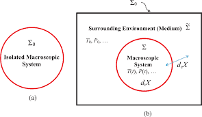
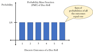
Up to now we have assumed that a random variable $\xi$, with entropy $H_{\xi}$, can take values from some discrete space consisting of either a finite or a countable number of elements, for instance, messages, symbols, etc. However, continuous variables are also widespread in engineering, i.e. variables (scalar or vector), which can take values from a continuous space $X$, most often from the space of real numbers. Such a random variable $\xi$ is described by the probability density function $p(\xi)$ that assigns the probability
$$
\Delta P=\int_{\xi \varepsilon \Delta X} p(\xi) d \xi \approx p(A) \Delta V \quad(A \in \Delta X)
$$
of $\xi$ appearing in region $\Delta X$ of the specified space $X$ with volume $\Delta V(d \xi=d V$ is a differential of the volume).

How can we define entropy $H_{\xi}$ for such a random variable? One of many possible formal ways is the following: In the formula
$$
H_{\xi}=-\sum_{\xi} P \xi \ln P(\xi)=-\mathbb{E}[\ln P(\xi)]
$$
appropriate for a discrete variable we formally replace probabilities $P(\xi)$ in the argument of the logarithm by the probability density and, thereby, consider the expression
$$
H_{\xi}=-\mathbb{E}[\ln p(\xi)]=-\int_{x} p(\xi) \ln p(\xi) d \xi .
$$
This way of defining entropy is not well justified. It remains unclear how to define entropy in the combined case, when a continuous distribution in a continuous space coexists with concentrations of probability at single points, i.e. the probability density contains delta-shaped singularities. Entropy (1.6.2) also suffers from the drawback that it is not invariant, i.e. it changes under a non-degenerate transformation of variables $\eta=f(\xi)$ in contrast to entropy (1.6.1), which remains invariant under such transformations.

数学代写|信息论代写information theory代考|Properties of entropy in the generalized version

Entropy (1.6.13), (1.6.16) defined in the previous section possesses a set of properties, which are analogous to the properties of an entropy of a discrete random variable considered earlier. Such an analogy is quite natural if we take into account the interpretation of entropy (1.6.13) (provided in Section 1.6) as an asymptotic case (for large $N$ ) of entropy (1.6.1) of a discrete random variable.

The non-negativity property of entropy, which was discussed in Theorem $1.1$, is not always satisfied for entropy (1.6.13), (1.6.16) but holds true for sufficiently large $N$. The constraint
$$
H_{\xi}^{P / Q} \leqslant \ln N
$$
results in non-negativity of entropy $H_{\xi}$.
Now we move on to Theorem $1.2$, which considered the maximum value of entropy. In the case of entropy (1.6.13), when comparing different distributions $P$ we need to keep measure $v$ fixed. As it was mentioned, quantity (1.6.17) is non-negative and, thus, (1.6.16) entails the inequality
$$
H_{\xi} \leqslant \ln N .
$$
At the same time, if we suppose $P=Q$, then, evidently, we will have
$$
H_{\xi}=\ln N .
$$
This proves the following statement that is an analog of Theorem $1.2$.

数学代写|信息论代写information theory代考|Encoding of discrete information

The definition of the amount of information, given in Chapter 1, is justified when we deal with a transformation of information from one kind into another, i.e. when considering encoding of information. It is essential that the law of conservation of information amount holds under such a transformation. It is very useful to draw an analogy with the law of conservation of energy. The latter is the main argument for introducing the notion of energy. Of course, the law of conservation of information is more complex than the law of conservation of energy in two respects. The law of conservation of energy establishes an exact equality of energies, when one type of energy is transformed into another. However, in transforming information we have a more complex relation, namely ‘not greater’ $(\leqslant)$, i.e. the amount of information cannot increase. The equality sign corresponds to optimal encoding. Thus, when formulating the law of conservation of information, we have to point out that there possibly exists such an encoding, for which the equality of the amounts of information occurs.

The second complication is that the equality is not exact. It is approximate, asymptotic, valid for complex (large) messages and for composite random variables. The larger a system of messages is, the more exact such a relation becomes. The exact equality sign takes place only in the limiting case. In this respect, there is an analogy with the laws of statistical thermodynamics, which are valid for large thermodynamic systems consisting of a large number (of the order of the Avogadro number) of molecules.

When conducting encoding, we assume that a long sequence of messages $\xi_{1}, \xi_{2}$, … is given together with their probabilities, i.e. a sequence of random variables. Therefore, the amount of information (entropy $H$ ) corresponding to this sequence can be calculated. This information can be recorded and transmitted by different realizations of the sequence. If $M$ is the number of such realizations, then the law of conservation of information can be expressed by the equality $H=\ln M$, which is complicated by the two above-mentioned factors (i.e. actually. $H \leqslant \ln M$ ).

Two different approaches may be used for solving the encoding problem. One can perform encoding of an infinite sequence of messages, i.e. online (or ‘sliding’) encoding. The inverse procedure, i.e. decoding, will be performed analogously.

信息论代考

数学代写|信息论代写information theory代考|Definition of entropy of a continuous random variable

到目前为止，我们假设一个随机变量 $\xi$, 有樀 $H_{\xi}$ ，可以从由有限或可数个元素组成的离散空间中取值，例如消息、
符号等。但是，连续变量在工程中也很普遍，即变量 (标量或向量)，它可以取来自连续空间的值 $X$ ，通常来自实数空间。这样的随机变量 $\xi$ 由概率密度函数描述 $p(\xi)$ 分配概率
$$
\Delta P=\int_{\xi \varepsilon \Delta X} p(\xi) d \xi \approx p(A) \Delta V \quad(A \in \Delta X)
$$
的 $\xi$ 出现在地区 $\Delta X$ 指定空间的 $X$ 有音量 $\Delta V(d \xi=d V$ 是体积的微分 $)$ 。
我们如何定义嫡 $H_{\xi}$ 对于这样一个随机变量? 许多可能的正式方式之一如下：在公式中
$$
H_{\xi}=-\sum_{\xi} P \xi \ln P(\xi)=-\mathbb{E}[\ln P(\xi)]
$$
适用于离散变量，我们正式替换概率 $P(\xi)$ 在概率密度的对数参数中，因此，考虑表达式
$$
H_{\xi}=-\mathbb{E}[\ln p(\xi)]=-\int_{x} p(\xi) \ln p(\xi) d \xi
$$
这种定义樀的方式是不合理的。目前尚不清楚如何在组合情况下定义熵，当连续空间中的连续分布与单个点的概率集中共存时，即概率密度包含三角形奇点。熵 (1.6.2) 也有一个缺点，即它不是不变的，即它在变量的非退化变换下变化 $\eta=f(\xi)$ 与熵 $(1.6 .1)$ 相反，熵在这种变换下保持不变。

数学代写|信息论代写information theory代考|Properties of entropy in the generalized version

上节定义的熵(1.6.13)、(1.6.16)具有一组性质，类似于前面考虑的离散随机变量的熵的性质。如果我们考虑将樀 (1.6.13) (在 $1.6$ 节中提供) 解释为渐近情况 (对于大 $N$ ) 的离散随机变量的嫡 (1.6.1)。
樀的非负性，在定理中讨论过 $1.1$ ，对于樀 (1.6.13), (1.6.16) 并不总是满足，但对于足够大的樀也成立 $N$. 约束
$$
H_{\xi}^{P / Q} \leqslant \ln N
$$
导致嫡的非负性 $H_{\xi}$.
现在我们继续讨论定理 $1.2$ ，它考虑了嫡的最大值。在熵 (1.6.13) 的情况下，当比较不同的分布时 $P$ 我们需要保持测量 $v$ 固定的。如前所述，数量 (1.6.17) 是非负的，因此，(1.6.16) 包含不等式
$$
H_{\xi} \leqslant \ln N \text {. }
$$
同时，如果我们假设 $P=Q$ ，那么，显然，我们将有
$$
H_{\xi}=\ln N .
$$
这证明了以下与定理类似的陈述 $1.2$.

数学代写|信息论代写information theory代考|Encoding of discrete information

第 1 章中给出的信息量定义在我们处理信息从一种类型到另一种类型的转换时是合理的，即在考虑信息编码时。在这种转变下，信息量守恒定律必须成立。与能量守恒定律进行类比是非常有用的。后者是引入能量概念的主要论据。当然，信息守恒定律在两个方面比能量守恒定律更复杂。当一种能量转化为另一种能量时，能量守恒定律确立了能量的精确相等性。然而，在转换信息时，我们有一个更复杂的关系，即“不是更大” $(\leqslant)$ ，即信息量不能增加。等号对应于最佳编码。因此，在制定信息守恒定律时，我们必须指出，可能存在这样一种编码，其信息量相等。
第二个复杂因素是等式并不精确。它是近似的、渐近的，对复杂 (大) 消息和复合随机变量有效。消息系统越大，这种关系就越精确。确切的等号仅在极限情况下出现。在这方面，与统计热力学定律有一个类比，该定律适用于由大量 (阿伏伽德罗数级) 分子组成的大型热力学系统。
在进行编码时，我们假设一长串消息 $\xi_{1}, \xi_{2}, \ldots$ 连同它们的概率一起给出，即一系列随机变量。因此，信息量（樀 $H)$ 对应这个序列可以计算出来。该信息可以通过序列的不同实现来记录和传输。如果 $M$ 是这种实现的数量，则信息守恒定律可以表示为等式 $H=\ln M$ ，这因上述两个因素而变得复杂（即实际上。 $H \leqslant \ln M$ ).
可以使用两种不同的方法来解决编码问题。可以对无限的消息序列进行编码，即在线 (或”滑动”) 编码。将类似地执行相反的过程，即解码。

数学代写|信息论代写information theory代考请认准statistics-lab™

统计代写请认准statistics-lab™. statistics-lab™为您的留学生涯保驾护航。

金融工程代写

金融工程是使用数学技术来解决金融问题。金融工程使用计算机科学、统计学、经济学和应用数学领域的工具和知识来解决当前的金融问题，以及设计新的和创新的金融产品。

非参数统计代写

非参数统计指的是一种统计方法，其中不假设数据来自于由少数参数决定的规定模型；这种模型的例子包括正态分布模型和线性回归模型。

广义线性模型代考

广义线性模型（GLM）归属统计学领域，是一种应用灵活的线性回归模型。该模型允许因变量的偏差分布有除了正态分布之外的其它分布。

术语广义线性模型（GLM）通常是指给定连续和/或分类预测因素的连续响应变量的常规线性回归模型。它包括多元线性回归，以及方差分析和方差分析（仅含固定效应）。

有限元方法代写

有限元方法（FEM）是一种流行的方法，用于数值解决工程和数学建模中出现的微分方程。典型的问题领域包括结构分析、传热、流体流动、质量运输和电磁势等传统领域。

有限元是一种通用的数值方法，用于解决两个或三个空间变量的偏微分方程（即一些边界值问题）。为了解决一个问题，有限元将一个大系统细分为更小、更简单的部分，称为有限元。这是通过在空间维度上的特定空间离散化来实现的，它是通过构建对象的网格来实现的：用于求解的数值域，它有有限数量的点。边界值问题的有限元方法表述最终导致一个代数方程组。该方法在域上对未知函数进行逼近。[1] 然后将模拟这些有限元的简单方程组合成一个更大的方程系统，以模拟整个问题。然后，有限元通过变化微积分使相关的误差函数最小化来逼近一个解决方案。

tatistics-lab作为专业的留学生服务机构，多年来已为美国、英国、加拿大、澳洲等留学热门地的学生提供专业的学术服务，包括但不限于Essay代写，Assignment代写，Dissertation代写，Report代写，小组作业代写，Proposal代写，Paper代写，Presentation代写，计算机作业代写，论文修改和润色，网课代做，exam代考等等。写作范围涵盖高中，本科，研究生等海外留学全阶段，辐射金融，经济学，会计学，审计学，管理学等全球99%专业科目。写作团队既有专业英语母语作者，也有海外名校硕博留学生，每位写作老师都拥有过硬的语言能力，专业的学科背景和学术写作经验。我们承诺100%原创，100%专业，100%准时，100%满意。

随机分析代写

随机微积分是数学的一个分支，对随机过程进行操作。它允许为随机过程的积分定义一个关于随机过程的一致的积分理论。这个领域是由日本数学家伊藤清在第二次世界大战期间创建并开始的。

时间序列分析代写

随机过程，是依赖于参数的一组随机变量的全体，参数通常是时间。随机变量是随机现象的数量表现，其时间序列是一组按照时间发生先后顺序进行排列的数据点序列。通常一组时间序列的时间间隔为一恒定值（如1秒，5分钟，12小时，7天，1年），因此时间序列可以作为离散时间数据进行分析处理。研究时间序列数据的意义在于现实中，往往需要研究某个事物其随时间发展变化的规律。这就需要通过研究该事物过去发展的历史记录，以得到其自身发展的规律。

回归分析代写

多元回归分析渐进（Multiple Regression Analysis Asymptotics）属于计量经济学领域，主要是一种数学上的统计分析方法，可以分析复杂情况下各影响因素的数学关系，在自然科学、社会和经济学等多个领域内应用广泛。

MATLAB代写

MATLAB 是一种用于技术计算的高性能语言。它将计算、可视化和编程集成在一个易于使用的环境中，其中问题和解决方案以熟悉的数学符号表示。典型用途包括：数学和计算算法开发建模、仿真和原型制作数据分析、探索和可视化科学和工程图形应用程序开发，包括图形用户界面构建MATLAB 是一个交互式系统，其基本数据元素是一个不需要维度的数组。这使您可以解决许多技术计算问题，尤其是那些具有矩阵和向量公式的问题，而只需用 C 或 Fortran 等标量非交互式语言编写程序所需的时间的一小部分。MATLAB 名称代表矩阵实验室。MATLAB 最初的编写目的是提供对由 LINPACK 和 EISPACK 项目开发的矩阵软件的轻松访问，这两个项目共同代表了矩阵计算软件的最新技术。MATLAB 经过多年的发展，得到了许多用户的投入。在大学环境中，它是数学、工程和科学入门和高级课程的标准教学工具。在工业领域，MATLAB 是高效研究、开发和分析的首选工具。MATLAB 具有一系列称为工具箱的特定于应用程序的解决方案。对于大多数 MATLAB 用户来说非常重要，工具箱允许您学习和应用专业技术。工具箱是 MATLAB 函数（M 文件）的综合集合，可扩展 MATLAB 环境以解决特定类别的问题。可用工具箱的领域包括信号处理、控制系统、神经网络、模糊逻辑、小波、仿真等。

R语言代写	问卷设计与分析代写
PYTHON代写	回归分析与线性模型代写
MATLAB代写	方差分析与试验设计代写
STATA代写	机器学习/统计学习代写
SPSS代写	计量经济学代写
EVIEWS代写	时间序列分析代写
EXCEL代写	深度学习代写
SQL代写	各种数据建模与可视化代写

数学代写|信息论代写information theory代考|ELEN90030

Posted on 2022年6月30日2022年6月30日 by statistics-lab

如果你也在怎样代写信息论information theory这个学科遇到相关的难题，请随时右上角联系我们的24/7代写客服。

我们提供的信息论information theory及其相关学科的代写，服务范围广, 其中包括但不限于:

Statistical Inference 统计推断
Statistical Computing 统计计算
Advanced Probability Theory 高等概率论
Advanced Mathematical Statistics 高等数理统计学
(Generalized) Linear Models 广义线性模型
Statistical Machine Learning 统计机器学习
Longitudinal Data Analysis 纵向数据分析
Foundations of Data Science 数据科学基础

数学代写|信息论代写information theory代考|ELEN90030

数学代写|信息论代写information theory代考|Conditional entropy. Hierarchical additivity

Let us generalize formulae (1.2.1), (1.2.3) to the case of conditional probabilities. Let $\xi_{1}, \ldots, \xi_{n}$ be random variables described by the joint distribution $P\left(\xi_{1}, \ldots, \xi_{n}\right)$. The conditional probabilities
$$
P\left(\xi_{k}, \ldots, \xi_{n} \mid \xi_{1}, \ldots, \xi_{k-1}\right)=\frac{P\left(\xi_{1}, \ldots, \xi_{n}\right)}{P\left(\xi_{1}, \ldots, \xi_{k-1}\right)} \quad(k \leqslant n)
$$
are associated with the random conditional entropy
$$
H\left(\xi_{k}, \ldots, \xi_{n} \mid \xi_{1}, \ldots, \xi_{k-1}\right)=-\ln P\left(\xi_{k}, \ldots, \xi_{n} \mid \xi_{1}, \ldots, \xi_{k-1}\right)
$$
Let us introduce a special notation for the result of averaging (1.3.1) over $\xi_{k}, \ldots, \xi_{n}$ :
$$
\begin{aligned}
H_{\xi_{k} \ldots \xi_{n}}\left(\mid \xi_{1}, \ldots \xi_{k-1}\right)=-\sum_{\xi_{k} \ldots \xi_{n}} P\left(\xi_{k}, \ldots\right.&\left., \xi_{n} \mid \xi_{1}, \ldots, \xi_{k-1}\right) \times \
& \times \ln P\left(\xi_{k}, \ldots, \xi_{n} \mid \xi_{1}, \ldots, \xi_{k-1}\right)
\end{aligned}
$$ and also for the result of total averaging:
$$
\begin{aligned}
H_{\xi_{k}, \ldots, \xi_{n}} \mid \xi_{1}, \ldots, \xi_{k-1} &=\mathbb{E}\left[H\left(\xi_{k}, \ldots, \xi_{n} \mid \xi_{1}, \ldots, \xi_{k-1}\right)\right] \
&=-\sum_{\xi_{1} \ldots \xi_{n}} P\left(\xi_{1} \ldots \xi_{n}\right) \ln P\left(\xi_{k}, \ldots, \xi_{n} \mid \xi_{1}, \ldots, \xi_{k-1}\right)
\end{aligned}
$$
If, in addition, we vary $k$ and $n$, then we will form a large number of different entropies, conditional and non-conditional, random and non-random. They are related by identities that will be considered below.

Before we formulate the main hierarchical equality (1.3.4), we show how to introduce a hierarchical set of random variables $\xi_{1}, \ldots, \xi_{n}$, even if there was just one random variable $\xi$ initially.

Let $\xi$ take one of $M$ values with probabilities $P(\xi)$. The choice of one realization will be made in several stages. At the first stage, we indicate which subset (from a full ensemble of non-overlapping subsets $E_{1}, \ldots, E_{m_{1}}$ ) the realization belongs to. Let $\xi_{1}$ be the index of such a subset. At the second stage, each subset is partitioned into smaller subsets $E_{\xi_{1} \xi_{2}}$. The second random variable $\xi_{2}$ points to which smaller subset the realization of the random variable belongs to. In turn, those smaller subsets are further partitioned until we obtain subsets consisting of a single element. Apparently, the number of nontrivial partitioning stages $n$ cannot exceed $M-1$. We can juxtapose a fixed partitioning scheme with a ‘decision tree’ depicted on Figure 1.1. Further considerations will be associated with a particular selected ‘tree’.

数学代写|信息论代写information theory代考|Asymptotic equivalence of non-equiprobable

The idea that the general case of non-equiprobable outcomes can be asymptotically reduced to the case of equiprobable outcomes is fundamental for information theory in the absence of noise. This idea belongs to Ludwig Boltzmann who derived formula (1.2.3) for entropy. Claude Shannon revived this idea and broadly used it for derivation of new results.

In considering this question here, we shall not try to reach generality, since these results form a particular case of more general results of Section 1.5. Consider the set of independent realizations $\eta=\left(\xi_{1}, \ldots, \xi_{n}\right)$ of a random variable $\xi=\xi_{j}$, which assumes one of two values 1 or 0 with probabilities $P[\xi=1]=p<1 / 2 ; P[\xi=$ $0]=1-p=q$. Evidently, the number of such different combinations (realizations) is equal to $2^{n}$. Let realization $\eta_{n_{1}}$ contain $n_{1}$ ones and $n-n_{1}=n_{0}$ zeros. Then its probability is given by
$$
P\left(\eta_{n_{1}}\right)=p^{n_{1}} q^{n-n_{1}}
$$
Of course, these probabilities are different for different $n_{1}$. The ratio $P\left(\eta_{0}\right) / P\left(\eta_{n}\right)=$ $(q / p)^{n}$ of the largest probability to the smallest one is big and increases fast with a growth of $n$. What equiprobability can we talk about then? The thing is that due to the Law of Large Numbers the number of ones $n_{1}=\xi_{1}+\cdots+\xi_{n}$ has a tendency to take values, which are close to its mean
$$
\mathbb{E}\left[n_{1}\right]=\sum_{j=1}^{n} \mathbb{E}\left[\xi_{j}\right]=n \mathbb{E}\left[\xi_{j}\right]=n p
$$

数学代写|信息论代写information theory代考|Asymptotic equiprobability and entropic stability

The ideas of preceding section concerning asymptotic equivalence of nonequiprobable and equiprobable outcomes can be extended to essentially more general cases of random sequences and processes. It is not necessary for random variables $\xi_{j}$ forming the sequence $\eta^{n}=\left(\xi_{1}, \ldots, \xi_{n}\right)$ to take only one of two values and to have the same distribution law $P\left(\xi_{j}\right)$. There is also no need for $\xi_{j}$ to be statistically independent and even for $\eta^{n}$ to be the sequence $\left(\xi_{1}, \ldots, \xi_{n}\right)$. So what is really necessary, the asymptotic equivalence?

In order to state the property of asymptotic equivalence of non-equiprobable and equiprobable outcomes in general terms we should use the notion of entropic stability of family of random variables.

A family of random variables $\left{\eta^{n}\right}$ is entropically stable if the ratio $H\left(\eta^{n}\right) / H_{\eta^{n}}$ converges in probability to one as $n \rightarrow \infty$. This means that whatever $\varepsilon>0, \eta>0$ are, there exists $N(\varepsilon, \eta)$ such that the inequality
$$
P\left{\left|H\left(\eta^{n}\right) / H_{\eta^{n}}-1\right| \geqslant \varepsilon\right}<\eta
$$
is satisfied for every $n \geqslant N(\varepsilon, \eta)$.
The above definition implies that $0<H_{\eta^{n}}<\infty$ and $H_{\eta^{n}}$ does not decrease with
$n$. Usually $H_{\eta^{n}} \rightarrow \infty$.
Asymptotic equiprobability can be expressed in terms of entropic stability in the form of the following general theorem.

Theorem 1.9. If a family of random variables $\left{\eta^{n}\right}$ is entropically stable, then the set of realizations of each random variable can be partitioned into two subsets $A_{n}$ and $B_{n}$ in such a way that

The total probability of realizations from subset $A_{n}$ vanishes:
$$
P\left(A_{n}\right) \rightarrow 0 \quad \text { as } \quad n \rightarrow \infty
$$

信息论代考

数学代写|信息论代写information theory代考|Conditional entropy. Hierarchical additivity

让我们将公式 (1.2.1)、(1.2.3) 推广到条件概率的情况。让 $\xi_{1}, \ldots, \xi_{n}$ 是由联合分布描述的随机变量 $P\left(\xi_{1}, \ldots, \xi_{n}\right)$. 条件概率
$$
P\left(\xi_{k}, \ldots, \xi_{n} \mid \xi_{1}, \ldots, \xi_{k-1}\right)=\frac{P\left(\xi_{1}, \ldots, \xi_{n}\right)}{P\left(\xi_{1}, \ldots, \xi_{k-1}\right)} \quad(k \leqslant n)
$$
与随机条件樀相关
$$
H\left(\xi_{k}, \ldots, \xi_{n} \mid \xi_{1}, \ldots, \xi_{k-1}\right)=-\ln P\left(\xi_{k}, \ldots, \xi_{n} \mid \xi_{1}, \ldots, \xi_{k-1}\right)
$$
让我们为平均 (1.3.1) 的结果引入一个特殊符号 $\xi_{k}, \ldots, \xi_{n}$ :
$$
H_{\xi_{k}, \ldots \xi_{n}}\left(\mid \xi_{1}, \ldots \xi_{k-1}\right)=-\sum_{\xi_{k} \ldots \xi_{n}} P\left(\xi_{k}, \ldots, \xi_{n} \mid \xi_{1}, \ldots, \xi_{k-1}\right) \times \quad \times \ln P\left(\xi_{k}, \ldots, \xi_{n} \mid \xi_{1}, \ldots, \xi_{k-1}\right)
$$
以及总平均的结果:
$$
H_{\xi_{k}, \ldots, \xi_{n}} \mid \xi_{1}, \ldots, \xi_{k-1}=\mathbb{E}\left[H\left(\xi_{k}, \ldots, \xi_{n} \mid \xi_{1}, \ldots, \xi_{k-1}\right)\right]=-\sum_{\xi_{1} \ldots \xi_{n}} P\left(\xi_{1} \ldots \xi_{n}\right) \ln P\left(\xi_{k}, \ldots, \xi_{n}\right.
$$
此外，如果我们改变 $k$ 和 $n$ ，那么我们就会形成大量不同的樀，有条件的和无条件的，随机的和非随机的。它们通过将在下面考虑的身份相关联。
在我们制定主要的分层等式 (1.3.4) 之前，我们展示了如何引入一组分层的随机变量 $\xi_{1}, \ldots, \xi_{n}$ ，即使只有一个随机变量 $\xi$ 最初。
让 $\xi$ 取其中之一 $M$ 带有概率的值 $P(\xi)$. 一种实现方式的选择将分几个阶段进行。在第一阶段，我们指出哪个子集 (来自非重鴐子集的完整集合 $E_{1}, \ldots, E_{m_{1}}$ ) 实现属于。让 $\xi_{1}$ 是这样一个子集的索引。在第二阶段，每个子集被划分为更小的子集 $E_{\xi_{1} \xi_{2}}$. 第二个随机变量 $\xi_{2}$ 指向随机变量的实现属于哪个较小的子集。反过来，这些较小的子集被进一步划分，直到我们获得由单个元素组成的子集。显然，非平凡划分阶段的数量 $n$ 不能超过 $M-1$. 我们可以将一个固定的分区方案与图 $1.1$ 中描述的“决策树”并列。进一步的考虑将与特定选择的”树”相关联。

数学代写|信息论代写information theory代考|Asymptotic equivalence of non-equiprobable

在没有㘇声的情况下，非等概率结果的一般情况可以渐近简化为等概率结果的情况的想法是信息论的基础。这个想法属于路德维希玻尔兹曼，他推导出熵的公式 (1.2.3) 。Claude Shannon 重新提出了这个想法，并将其广泛用于推导新结果。
在这里考虑这个问题时，我们不会试图达到一般性，因为这些结果形成了 $1.5$ 节更一般性结果的一个特例。考虑一组独立的实现 $\eta=\left(\xi_{1}, \ldots, \xi_{n}\right)$ 随机变量 $\xi=\xi_{j}$ ，它假设两个值之一的概率为 1 或 0
$P[\xi=1]=p<1 / 2 ; P[\xi=0]=1-p=q$. 显然，这种不同组合（实现）的数量等于 $2^{n}$. 让实现 $\eta_{n_{1}}$ 包含 $n_{1}$ 一个和 $n-n_{1}=n_{0}$ 零。那么它的概率由下式给出
$$
P\left(\eta_{n_{1}}\right)=p^{n_{1}} q^{n-n_{1}}
$$
当然，这些概率对于不同的 $n_{1}$. 比例 $P\left(\eta_{0}\right) / P\left(\eta_{n}\right)=(q / p)^{n}$ 从最大概率到最小概率的概率很大，并且随着的增长而快速增加 $n$. 那么我们可以谈论什么等概率呢? 问题是由于大数定律 $n_{1}=\xi_{1}+\cdots+\xi_{n}$ 倾向于取接近平均值的值
$$
\mathbb{E}\left[n_{1}\right]=\sum_{j=1}^{n} \mathbb{E}\left[\xi_{j}\right]=n \mathbb{E}\left[\xi_{j}\right]=n p
$$

数学代写|信息论代写information theory代考|Asymptotic equiprobability and entropic stability

上一节关于非等概率和等概率结果的渐近等价的想法可以扩展到更一般的随机序列和过程的情况。随机变量不是必需的 $\xi_{j}$ 形成序列 $\eta^{n}=\left(\xi_{1}, \ldots, \xi_{n}\right)$ 只取两个值之一并具有相同的分布规律 $P\left(\xi_{j}\right)$. 也没有必要 $\xi_{j}$ 在统计上是独立的，甚至对于 $\eta^{n}$ 成为序列 $\left(\xi_{1}, \ldots, \xi_{n}\right)$. 那么什么是真正必要的，渐近等价呢?
为了概括地说明非等概率和等概率结果的渐近等价性质，我们应该使用随机变量族的嫡稳定性的概念。
随机变量族 Veft {leta^{n}\right } } \text { 如果比率是樀稳定的 } H ( \eta ^ { n } ) / H _ { \eta ^ { n } } \text { 在概率上收敛为 } 1 n \rightarrow \infty \text { . 这意味着无论 } $\varepsilon>0, \eta>0$ 是，存在 $N(\varepsilon, \eta)$ 这样不等式
P\left{\eft $\mid H \backslash l e f t(\mathrm{~ l e t a}$
满足于每一个 $n \geqslant N(\varepsilon, \eta)$.
上述定义意味着 $0<H_{\eta^{n}}<\infty$ 和 $H_{\eta^{n}}$ 不减少
$n$. 通常 $H_{\eta^{n}} \rightarrow \infty$.
渐近等概率可以用以下一般定理的形式用嫡稳定性表示。
$\mathrm{~ 定理 ~ 1 . 9 。如果一个随机变量族 l l e f t : n e t a ^ { n }}$ $A_{n}$ 和 $B_{n}$ 以这样的方式
子集实现的总概率 $A_{n}$ 消失:
$$
P\left(A_{n}\right) \rightarrow 0 \quad \text { as } \quad n \rightarrow \infty
$$

统计代写请认准statistics-lab™. statistics-lab™为您的留学生涯保驾护航。

金融工程代写

非参数统计代写

非参数统计指的是一种统计方法，其中不假设数据来自于由少数参数决定的规定模型；这种模型的例子包括正态分布模型和线性回归模型。

广义线性模型代考

广义线性模型（GLM）归属统计学领域，是一种应用灵活的线性回归模型。该模型允许因变量的偏差分布有除了正态分布之外的其它分布。

有限元方法代写

随机分析代写

时间序列分析代写

回归分析代写

MATLAB代写

R语言代写	问卷设计与分析代写
PYTHON代写	回归分析与线性模型代写
MATLAB代写	方差分析与试验设计代写
STATA代写	机器学习/统计学习代写
SPSS代写	计量经济学代写
EVIEWS代写	时间序列分析代写
EXCEL代写	深度学习代写
SQL代写	各种数据建模与可视化代写

数学代写|信息论代写information theory代考|COMP2610

Posted on 2022年6月30日2022年6月30日 by statistics-lab

如果你也在怎样代写信息论information theory这个学科遇到相关的难题，请随时右上角联系我们的24/7代写客服。

我们提供的信息论information theory及其相关学科的代写，服务范围广, 其中包括但不限于:

Statistical Inference 统计推断
Statistical Computing 统计计算
Advanced Probability Theory 高等概率论
Advanced Mathematical Statistics 高等数理统计学
(Generalized) Linear Models 广义线性模型
Statistical Machine Learning 统计机器学习
Longitudinal Data Analysis 纵向数据分析
Foundations of Data Science 数据科学基础

数学代写|信息论代写information theory代考|Definition of information and entropy in the absence of noise

In modern science, engineering and public life, a big role is played by information and operations associated with it: information reception, information transmission, information processing, storing information and so on. The significance of information has seemingly outgrown the significance of the other important factor, which used to play a dominant role in the previous century, namely, energy.

In the future, in view of a complexification of science, engineering, economics and other fields, the significance of correct control in these areas will grow and, therefore, the importance of information will increase as well.

What is information? Is a theory of information possible? Are there any general laws for information independent of its content that can be quite diverse? Answers to these questions are far from obvious. Information appears to be a more difficult concept to formalize than, say, energy, which has a certain, long established place in physics.

There are two sides of information: quantitative and qualitative. Sometimes it is the total amount of information that is important, while other times it is its quality, its specific content. Besides, a transformation of information from one format into another is technically a more difficult problem than, say, transformation of energy from one form into another. All this complicates the development of information theory and its usage. It is quite possible that the general information theory will not bring any benefit to some practical problems, and they have to be tackled by independent engineering methods.

Nevertheless, general information theoory exists, and so dō standärd situations and problems, in which the laws of general information theory play the main role. Therefore, information theory is important from a practical standpoint, as well as in fundamental science, philosophy and expanding the horizons of a researcher.

From this introduction one can gauge how difficult it was to discover the laws of information theory. In this regard, the most important milestone was the work of Claude Shannon $[44,45]$ published in 1948-1949 (the respective English originals are $[38,39]$ ). His formulation of the problem and results were both perceived as a surprise. However, on closer investigation one can see that the new theory extends and develops former ideas, specifically, the ideas of statistical thermodynamics due to Boltzmann. The deep mathematical similarities between these two directions are not accidental. It is evidenced in the use of the same formulae (for instance, for entropy of a discrete random variable). Besides that, a logarithmic measure for the amount of information, which is fundamental in Shannon’s theory, was proposed for problems of communication as early as 1928 in the work of R. Hartley [19] (the English original is [18]).

In the present chapter, we introduce the logarithmic measure of the amount of information and state a number of important properties of information, which follow from that measure, such as the additivity property.

The notion of the amount of information is closely related to the notion of entropy, which is a measure of uncertainty. Acquisition of information is accompanied by a decrease in uncertainty, so that the amount of information can be measured by the amount of uncertainty or entropy that has disappeared.

In the case of a discrete message, i.e. a discrete random variable, entropy is defined by the Boltzmann formula
$$
H_{\xi}=-\sum_{\xi} P(\xi) \ln P(\xi),
$$
where $\xi$ is a random variable, and $P(\xi)$ is its probability distribution.

数学代写|信息论代写information theory代考|Definition of entropy in the case of equiprobable outcomes

Suppose we have $M$ equiprobable outcomes of an experiment. For example, when we roll a standard die, $M=6$. Of course, we cannot always perform the formalization of conditions so easily and accurately as in the case of a die. We assume though that the formalization has been performed and, indeed, one of $M$ outcomes is realized, and they are equivalent in probabilistic terms. Then there is a priori uncertainty directly connected with $M$ (i.e. the greater the $M$ is, the higher the uncertainty is). The quantity measuring the above uncertainty is called entropy and is denoted by $H:$
$$
H=f(M),
$$
where $f(\cdot)$ is some increasing non-negative function defined at least for natural numbers.

When rolling a dice and observing the outcome number, we obtain information whose amount is denoted by $I$. After that (i.e. a posteriori) there is no uncertainty left: the a posteriori number of outcomes is $M=1$ and we must have $H_{\mathrm{ps}}=f(1)=0$. It is natural to measure the amount of information received by the value of disappeared uncertainty:
$$
I=H_{\mathrm{pr}}-H_{\mathrm{ps}} .
$$
Here, the subscript ‘pr’ means ‘a priori’, whereas ‘ps’ means ‘a posteriori’.
We see that the amount of received information $I$ coincides with the initial entropy. In other cases (in particular, for formula (1.2.3) given below) a message having entropy $H$ can also transmit the amount of information $I$ equal to $H$.

In order to determine the form of function $f(\cdot)$ in (1.1.1) we employ very natural additivity principle. In the case of a die it reads: the entropy of two throws of a die is twice as large as the entropy of one throw, the entropy of three throws of a die is three times as large as the entropy of one throw, etc. Applying the additivity principle to other cases means that the entropy of several independent systems is equal to the sum of the entropies of individual systems. However, the number $M$ of outcomes for a complex system is equal to the product of the numbers $m$ of outcomes for each one of the ‘simple’ (relative to the total system) subsystems. For two throws of dice, the number of various pairs $\left(\xi_{1}, \xi_{2}\right)$ (where $\xi_{1}$ and $\xi_{2}$ both take one out of six values) equals to $36=6^{2}$. Generally, for $n$ throws the number of equivalent outcomes is $6^{n}$. Applying formula (1.1.1) for this number, we obtain entropy $f\left(6^{n}\right)$. According to the additivity principle, we find that
$$
f\left(6^{n}\right)=n f(6)
$$

数学代写|信息论代写information theory代考|Entropy and its properties in the case of non-equiprobable outcomes

Suppose now the probabilities of different outcomes are unequal. If, as earlier, the number of outcomes equals to $M$, then we can consider a random variable $\xi$, which takes one of $M$ values. Considering an index of the corresponding outcome as $\xi$, we obtain that those values are nothing else but $1, \ldots, M$. Probabilities $P(\xi)$ of those values are non-negative and satisfy the normalization constraint: $\sum_{\xi} P(\xi)=1$.

If we formally apply equality (1.1.8) to this case, then each $\xi$ should have its own entropy
$$
H(\xi)=-\ln P(\xi) .
$$
Thus, we attribute a certain value of entropy to each realization of the variable $\xi$. Since $\xi$ is a random variable, we can also regard this entropy as a random variable.
As in Section 1.1, the a posteriori entropy, which remains after the realization of $\xi$ becomes known, is equal to zero. That is why the information we obtain once the realization is known is numerically equal to the initial entropy
$$
I(\xi)=H(\xi)=-\ln P(\xi)
$$
Similar to entropy $H(\xi)$, information $I$ depends on the actual realization (on the value of $\xi$ ), i.e., it is a random variable. One can see from the latter formula that information and entropy are both large when a posteriori probability of the given realization is small and vice versa. This observation is quite consistent with intuitive ideas.

Example 1.1. Suppose we would like to know whether a certain student has passed an exam or not. Let the probabilities of these two events be
$$
P(\text { pass })=7 / 8, \quad P(\text { fail })=1 / 8
$$
One can see from these probabilities that the student is quite strong. If we were informed that the student had passed the exam, then we could say: ‘Your message has not given me a lot of information. I have already expected that the student passed the exam’. According to formula (1.2.2) the information of this message is quantitatively equal to
$$
I(\text { pass })=\log {2}(8 / 7)=0.193 \text { bits. } $$ If we were informed that the student had failed, then we would say ‘Really?’ and would feel that we have improved our knowledge to a greater extent. The amount of information of such a message is equal to $$ I(\text { fail })=\log {2}(8)=3 \text { bits. }
$$

信息论代考

数学代写|信息论代写information theory代考|Definition of information and entropy in the absence of noise

在现代科学、工程和公共生活中，信息及其相关操作发挥着重要作用：信息接收、信息传输、信息处理、信息存储等。信息的重要性似乎已经超过了另一个重要因溸的重要性，后者在上个世纪曾占据主导地位，即能源。
末来，随着科学、工程、经济等领域的笪杂化，这些领域的正确控制的意义将越来越大，因此信息的重要性也将越来越大o
什么是信息? 信息理论可能吗? 是否有任何独立于其内容的信息的一般规律，可以是非常多样化的? 这些问题的答案远非显而易见。与能量相比，信息似乎是一个更难形式化的概念，能量在物理学中具有一定的、长期确立的地位。
信息有两个方面：定量和定性。有时重要的是信息的总量，而有时则是它的质量，它的具体内容。此外，从一种形式到另一种形式的信息转换在技术上比从一种形式到另一种形式的能量转换更困难。所有这些都使信息论的发展及其使用变得复杂。一般信息论很可能对一些实际问题没有任何好处，必须通过独立的工程方法来解决。
但是，一般信息论是存在的，标准的情况和问题也是存在的，其中一般信息论的规律起主要作用。因此，从实践的角度来看，信息论以及在基础科学、哲学和扩展研究人员的视野方面都很重要。
从这个介绍可以看出发现信息论定律有多么困难。在这方面，最重要的里程碑是克劳德自农的工作 $[44,45]$ 出版于 19481949 年（各自的英文原件是 $[38,39]$ )。他对问题的表述和结果都被认为是一个掠喜。然而，通过更深入的研究，我们] 可以看到新理论扩展和发展了以前的思想，特别是玻尔兹曼的统计热力学思想。䢒两个方向之间在数学上的深刻相似性并非偶然。使用相同的公式就证明了这一点（例如，对于离散随机六量的熵）。除此之外，早在 1928 年，R. Hartley [19] (英文原版为 [18]) 就提出了用于解决通信问题的信息量的对数度量，这是香农理论中的基础。
在本章中，我们介绍了信息量的对数度量，并说明了信息的一些重要属性，这些属性是从该度量得出的，例如可加性。
信息量的概念与熵的概念密切相关，熵是不确定性的度量。信息的获取伴随着不确定性的减少，因此信息量可以通过已经消失的不确定性或熵的量来衡量。
在离散消息的情况下，即禽散随机变量，熵由玻尔兹曼公式定义
$$
H_{\xi}=-\sum_{\xi} P(\xi) \ln P(\xi)
$$
在哪里 $\xi$ 是一个随机变量，并且 $P(\xi)$ 是它的概率分布。

数学代写|信息论代写information theory代考|Definition of entropy in the case of equiprobable outcomes

假设我们有 $M$ 实验的等概率结果。例如，当我们烪出一个标准㱿子时， $M=6$. 当然，我们不能总是像在骰子的情况下那样容易和准确地执行条件的形式化。我们假设虽然形式化已经执行，并且实际上，其中之一 $M$ 结果是实现的，并且它们在概率方面是等价的。那么有一个先验的不确定性直接与 $M$ (即越大 $M$ 是，不确定性越高) 。测量上述不确定性的量称为熵，表示为 $H$ :
$$
H=f(M),
$$
在哪里 $f(\cdot)$ 是至少为自然数定义的一些递增的非负函数。
当掷骰子并观崇结果数时，我们获得的信息量表示为 $I$. 在那之后（即后验），就没有不确定性了：结果的后验数量是 $M=1$ 我们必须有 $H_{\mathrm{ps}}=f(1)=0$. 通过消失的不确定性的值来衡量接收到的信息量是很自然的:
$$
I=H_{\mathrm{pr}}-H_{\mathrm{ps}} .
$$
这里，下标”pr”表示”先验”，而“ps”表示”后验”。
我们看到接收到的信息量 $I$ 与初始熵一致。在其他情况下（特别是对于下面给出的公式 (1.2.3) ）具有熵的消自 $H$ 还可以传递信息量 $I$ 等于 $H$.
为了确定函数的形式 $f(\cdot)$ 在 (1.1.1) 中，我们采用了非常自然的可加性原理。在䁊子的情况下，它读作：两次掷骰子的熵是一次掷骰子的熵的两倍，三次掷猒子的熵是一次掷刕子的熵的三倍，等等。将可加性原理应用于其他情况意味着几个独立系统的熵等于各个系统的熵之和。然而，数 $M$ 复杂系统的结果等于数字的乘积 $m$ 每个”简单”（相对于整个系统）子系统的结果。对于两次掷骰子，各种对的数量 $\left(\xi_{1}, \xi_{2}\right)$ (在哪里 $\xi_{1}$ 和 $\xi_{2}$ 都取六个值中的一个) 等于 $36=6^{2}$. 一般来说，对于 $n$ 抛出等效结果的数量是 $6^{n}$. 对这个数应用公式 (1.1.1)，我们得到熵 $f\left(6^{n}\right)$. 根据可加性原理，我们发现
$$
f\left(6^{n}\right)=n f(6)
$$

数学代写|信息论代写information theory代考|Entropy and its properties in the case of non-equiprobable outcomes

假设现在不同结果的概率不相等。如果如前所述，结果的数量等于 $M$ ，那么我们可以考虑一个随机变量 $\xi$ ，它需要一个 $M$ 价值观。将相应结果的索引视为 $\xi$ ，我们得到这些值只不过是 $1, \ldots, M$. 概率 $P(\xi)$ 这些值中的一个是非负的并且满足规范化约束: $\sum_{\xi} P(\xi)=1$.
如果我们正式将等式 (1.1.8) 应用于这种情况，那么每个 $\xi$ 应该有自己的熵
$$
H(\xi)=-\ln P(\xi) .
$$
因此，我们将某个熵值赋予变量的每个实现 $\xi$. 自从 $\xi$ 是一个随机变量，我们也可以把这个熵看作一个随机变量。与第 $1.1$ 节一样，后验樀在实现 $\xi$ 变得已知，等于零。这就是为什么我们在实现已知后获得的信息在数值上等于初始樀
$$
I(\xi)=H(\xi)=-\ln P(\xi)
$$
类似于樀 $H(\xi)$ ，信自 $I$ 取决于实际实现（在价值 $\xi$ ，即它是一个随机变量。从后一个公式可以看出，当给定实现的后验概率很小时，信息和樀都很大，反之亦然。这种观眎与直觉的想法是相当一致的。
例 1.1。假设我们想知道某个学生是否通过了考试。让这两个事件的概率为
$$
P(\text { pass })=7 / 8, \quad P(\text { fail })=1 / 8
$$
从这些概率可以看出，学生的实力相当强。如果我们被告知学生通过了考试，那么我们可以说：’你的消自没有给我很多信息。我已经预料到学生会通过考试。”根据公式 (1.2.2)，这条消息的信息量等于
$$
I(\text { pass })=\log 2(8 / 7)=0.193 \text { bits. }
$$
如果殘们被告知学生失败了，那么我们会说“真的吗? “并且会觉得我们在更大程度上提高了我们的知识。这样一条消息的信息量等于
$$
I(\text { fail })=\log 2(8)=3 \text { bits. }
$$

统计代写请认准statistics-lab™. statistics-lab™为您的留学生涯保驾护航。

金融工程代写

非参数统计代写

非参数统计指的是一种统计方法，其中不假设数据来自于由少数参数决定的规定模型；这种模型的例子包括正态分布模型和线性回归模型。

广义线性模型代考

广义线性模型（GLM）归属统计学领域，是一种应用灵活的线性回归模型。该模型允许因变量的偏差分布有除了正态分布之外的其它分布。

有限元方法代写

随机分析代写

时间序列分析代写

回归分析代写

MATLAB代写

R语言代写	问卷设计与分析代写
PYTHON代写	回归分析与线性模型代写
MATLAB代写	方差分析与试验设计代写
STATA代写	机器学习/统计学习代写
SPSS代写	计量经济学代写
EVIEWS代写	时间序列分析代写
EXCEL代写	深度学习代写
SQL代写	各种数据建模与可视化代写

数学代写|信息论代写information theory代考|COMP2610

Posted on 2022年6月17日2022年6月18日 by statistics-lab

如果你也在怎样代写信息论information theory这个学科遇到相关的难题，请随时右上角联系我们的24/7代写客服。

我们提供的信息论information theory及其相关学科的代写，服务范围广, 其中包括但不限于:

Statistical Inference 统计推断
Statistical Computing 统计计算
Advanced Probability Theory 高等概率论
Advanced Mathematical Statistics 高等数理统计学
(Generalized) Linear Models 广义线性模型
Statistical Machine Learning 统计机器学习
Longitudinal Data Analysis 纵向数据分析
Foundations of Data Science 数据科学基础

数学代写|信息论代写information theory代考|Information Theory Re-founded and Re-envisioned

数学代写|信息论代写information theory代考|Quantum Information Theory Re-envisioned

This “classical” (i.e., non-quantum) logical information theory is developed with the data of two or more partitions (or random variables) on a set with point probabilities. The transition to the quantum case was guided by the method of linearizing set concepts to obtain the corresponding vector space concepts, which are then specialized to finite-dimensional Hilbert spaces. The underlying set is replaced by a basis set of simultaneous orthonormal eigenvectors of two or more commuting self-adjoint linear operators (observables), the partitions are replaced by the direct-sum decompositions of the eigenspaces of the operators, Cartesian products are replaced by tensor products, and the point probabilities are provided by the state to be measured. The first fundamental theorem for quantum logical entropy and measurement established a direct quantitative connection between the increase in quantum logical entropy due to a projective measurement and the eigenstates (cohered together in the pure superposition state being measured) that

are distinguished by the measurement (decohered in the post-measurement mixed state). This theorem establishes quantum logical entropy as a natural notion for a quantum information theory focusing on distinguishing states.

The classical theory may also be developed just using two probability distributions, $p=\left(p_{1}, \ldots, p_{n}\right)$ and $q=\left(q_{1}, \ldots, q_{n}\right)$, indexed by the same set, and this is generalized to the quantum case where we are just given two density matrices $\rho$ and $\tau$ representing two states in a Hilbert space. Then the Hamming distance can be carried over from the classical to the quantum case where it is equal to the Hilbert-Schmidt norm (square of the trace distance and quantum analogue of square of Euclidean distance). A second theorem relating measurement and logical entropy is that the Hilbert-Schmidt norm (= quantum logical Hamming distance) between any pre-measurement state $\rho$ and the state $\hat{\rho}$ resulting from a projective measurement of the state is just the difference in their logical entropies, $h(\hat{\rho})-h(\rho)$. There are other benefits of quantum logical entropy (as opposed to von Neumann entropy) emphasized by Manfredi and Feix [5] as well as Tamir and Cohen $[12,13]$ but our points focused on the natural connections with projective quantum measurement (described by the Lüders mixture operation) and notions of distance between quantum states, i.e., Hilbert-Schmidt norm $=$ Square of trace distance $=$ Quantum logical Hamming distance.

数学代写|信息论代写information theory代考|What Is to Be Done

This re-envisioning of information theory is probably controversial due in part to the role of logical entropy to directly measure information-as-distinctions. We have presented only bits and pieces of the intriguing connections between logical entropy and Shannon entropy, e.g., the dit-bit transform. There is work to be done to uncover the underlying mathematical theory that will fully account for those connections.
The results on Boltzmannian entropy in statistical mechanics and Shannon entropy in information theory were largely cautionary. Conceptual conclusions have been drawn from the role of Shannon entropy as a numerical approximation to Boltzmannian entropy, and that has engendered many confusions and overstatements in the literature.

We gave a few basic theorems relating quantum logical entropy to projective quantum measurement and to the Hilbert-Schmidt norm. Quantum information theory has seen enormous growth in the last half-century, so much work might be done to see how logical entropy relates to those results (e.g., [12] and [13]) and what new results can be obtained following the linearization methodology to relate classical results to quantum results. And there has been extensive and exhausting work following the seminal 1936 paper of Birkhoff and von Neumann [2] that first linearized the Boolean logic of subsets to the quantum logic of subspaces. But we have noted that the same linearization methodology linearizes the logic of partitions on sets (see the Appendix) to the logic of direct-sum decompositions of vector spaces which provides the dual form of quantum logic when specialized to Hilbert spaces-but that logic has barely been investigated [4].

数学代写|信息论代写information theory代考|Subset Logic and Partition Logic

Since logical entropy arises as the quantitative version of the logic of partitions just as logical or Laplacian probability arises as the quantitative version of the logic of subsets, this Appendix will give a few basics the logic of partitions $[5,6]$.

In classical propositional logic, the atomic variables and compound formulas are usually interpreted as representing propositions (see any textbook in logic). But in terms of mathematical entities, the variables and formulas may be taken as representing subsets of some fixed universe set $U(|U| \geq 1)$ with the propositional interpretation being identified with the special case of subsets $0=\emptyset$ and 1 of a one element set 1. Alonzo Church noted that George Boole and Augustus De Morgan originally interpreted logic as a logic of subsets or classes.
The algebra of logic has its beginning in 1847 , in the publications of Boole and De Morgan. This concerned itself at first with an algebra or calculus of classes, to which a similar algebra of relations was later added.[3, pp. 155-156]
Today, largely due to the efforts of F. William Lawvere, subsets were generalized to subobjects or “parts” (equivalence classes of monomorphisms) so that logic has become the logic of subobjects or parts in a topos (such as the category of sets). In the basic case of the category of sets, it is again the logic of subsets.

In view of the general subset interpretation, “Boolean logic” or “subset logic” would be a better name for what is usually called “propositional logic.” Using this subset interpretation of the connectives such as join, meet, and implication, then a tautology, herein Subset tautology, is any formula such that regardless of what subsets of $U$ are assigned to the atomic variables, the whole formula will evaluate to the universe set $U$. Remarkably, to define subset tautologies, it is sufficient (a fact known to Boole) to restrict attention to the two subsets of a singleton $U=1$ (or, equivalently, only the subsets $\emptyset$ and $U$ of a general $U$ ) which is done, in effect, in the usual propositional interpretation where tautologies are defined as truth-table tautologies. The truth-table notion of a tautology should be a theorem, not a definition; indeed it is a theorem that extends to valid probability formulas [12].

信息论代考

数学代写|信息论代写information theory代考|Quantum Information Theory Re-envisioned

这种“经典”（即非量子）逻辑信息论是利用具有点概率的集合上的两个或多个分区（或随机变量）的数据开发的。通过线性化集合概念的方法指导向量子情况的过渡，以获得相应的向量空间概念，然后将其专门化为有限维希尔伯特空间。基础集被两个或多个可交换自伴随线性算子（可观察量）的同时正交特征向量的基组替换，分区被算子的特征空间的直接和分解替换，笛卡尔积被张量替换产品，点概率由待测状态提供。

由测量区分（在测量后混合状态下分离）。该定理将量子逻辑熵确立为专注于区分状态的量子信息理论的自然概念。

经典理论也可以仅使用两个概率分布来发展，p=(p1,…,pn)和q=(q1,…,qn), 由同一个集合索引，这被推广到量子情况，我们只得到两个密度矩阵ρ和τ表示希尔伯特空间中的两个状态。然后，汉明距离可以从经典情况转移到等于希尔伯特-施密特范数（轨迹距离的平方和欧几里得距离平方的量子模拟）的量子情况。与测量和逻辑熵相关的第二个定理是任何预测量状态之间的希尔伯特-施密特范数（=量子逻辑汉明距离）ρ和国家ρ^由状态的投影测量产生的只是它们逻辑熵的差异，H(ρ^)−H(ρ). Manfredi 和 Feix [5] 以及 Tamir 和 Cohen 强调了量子逻辑熵（与 von Neumann 熵相反）的其他好处[12,13]但我们的观点集中在与射影量子测量的自然联系（由 Lüders 混合运算描述）和量子态之间的距离概念，即 Hilbert-Schmidt 范数=跟踪距离的平方=量子逻辑汉明距离。

数学代写|信息论代写information theory代考|What Is to Be Done

这种对信息论的重新构想可能是有争议的，部分原因是逻辑熵在直接测量信息作为区分方面的作用。我们只介绍了逻辑熵和香农熵之间有趣的联系的零碎部分，例如，dit-bit 变换。需要做一些工作来揭示能够充分解释这些联系的基本数学理论。
统计力学中的玻尔兹曼熵和信息论中的香农熵的结果在很大程度上是警示性的。从香农熵作为玻尔兹曼熵的数值近似的作用得出了概念性结论，这在文献中引起了许多混淆和夸大。

我们给出了一些将量子逻辑熵与射影量子测量和希尔伯特-施密特范数相关的基本定理。量子信息论在过去的半个世纪中取得了巨大的发展，可能需要做很多工作来了解逻辑熵与这些结果的关系（例如，[12] 和 [13]），以及在线性化之后可以获得哪些新结果将经典结果与量子结果联系起来的方法。在 Birkhoff 和 von Neumann [2] 的开创性论文 1936 年首次将子集的布尔逻辑线性化为子空间的量子逻辑之后，进行了广泛而艰巨的工作。

数学代写|信息论代写information theory代考|Subset Logic and Partition Logic

由于逻辑熵作为分区逻辑的定量版本出现，就像逻辑或拉普拉斯概率作为子集逻辑的定量版本出现一样，本附录将给出分区逻辑的一些基础知识[5,6].

在经典命题逻辑中，原子变量和复合公式通常被解释为代表命题（参见任何逻辑教科书）。但就数学实体而言，变量和公式可以看作是某个固定宇宙集的子集在(|在|≥1)命题解释与子集的特殊情况相同0=∅和一个元素集 1 中的 1 个。Alonzo Church 指出，George Boole 和 Augustus De Morgan 最初将逻辑解释为子集或类的逻辑。
逻辑代数始于 1847 年，在 Boole 和 De Morgan 的出版物中。这首先与类的代数或微积分有关，后来添加了类似的关系代数。 [3, pp. 155-156]
今天，很大程度上由于 F. William Lawvere 的努力，子集被推广到子对象或“部分”（单态的等价类），因此逻辑已成为拓扑中的子对象或部分的逻辑（例如集合的范畴）。在集合范畴的基本情况下，它又是子集的逻辑。

鉴于一般的子集解释，“布尔逻辑”或“子集逻辑”将是通常称为“命题逻辑”的更好名称。使用连接词的这个子集解释，例如连接、相遇和蕴涵，然后重言式，这里的子集重言式，是任何公式，无论是什么子集在分配给原子变量，整个公式将评估为宇宙集在. 值得注意的是，要定义子集重言式，将注意力限制在单例的两个子集上就足够了（布尔已知的事实）在=1（或者，等效地，只有子集∅和在一般的在) 这实际上是在通常的命题解释中完成的，其中重言式被定义为真值表重言式。重言式的真值表概念应该是一个定理，而不是一个定义；事实上，它是一个扩展到有效概率公式的定理 [12]。

统计代写请认准statistics-lab™. statistics-lab™为您的留学生涯保驾护航。

金融工程代写

非参数统计代写

非参数统计指的是一种统计方法，其中不假设数据来自于由少数参数决定的规定模型；这种模型的例子包括正态分布模型和线性回归模型。

广义线性模型代考

广义线性模型（GLM）归属统计学领域，是一种应用灵活的线性回归模型。该模型允许因变量的偏差分布有除了正态分布之外的其它分布。

有限元方法代写

随机分析代写

时间序列分析代写

回归分析代写

MATLAB代写

R语言代写	问卷设计与分析代写
PYTHON代写	回归分析与线性模型代写
MATLAB代写	方差分析与试验设计代写
STATA代写	机器学习/统计学习代写
SPSS代写	计量经济学代写
EVIEWS代写	时间序列分析代写
EXCEL代写	深度学习代写
SQL代写	各种数据建模与可视化代写

数学代写|信息论代写information theory代考|ELEN90030

Posted on 2022年6月17日2022年6月18日 by statistics-lab

如果你也在怎样代写信息论information theory这个学科遇到相关的难题，请随时右上角联系我们的24/7代写客服。

我们提供的信息论information theory及其相关学科的代写，服务范围广, 其中包括但不限于:

Statistical Inference 统计推断
Statistical Computing 统计计算
Advanced Probability Theory 高等概率论
Advanced Mathematical Statistics 高等数理统计学
(Generalized) Linear Models 广义线性模型
Statistical Machine Learning 统计机器学习
Longitudinal Data Analysis 纵向数据分析
Foundations of Data Science 数据科学基础

数学代写|信息论代写information theory代考|Quantum Logical Information Theory

数学代写|信息论代写information theory代考|Density Matrix Treatment of Logical Entropy

This section facilitates the transition to quantum logical information theory classical’ antecedents. It was previously noted that binary relation $R \subseteq U \times U$ on $U=\left{u_{1}, \ldots, u_{n}\right}$ can be represented by an $n \times n$ incidence matrix $\operatorname{In}(R)$ where
$$
\operatorname{In}(R){i j}=\left{\begin{array}{c} 1 \text { if }\left(u{i}, u_{j}\right) \in R \
0 \text { if }\left(u_{i}, u_{j}\right) \notin R
\end{array}\right.
$$

And then taking $R$ as the equivalence relation indit $(\pi)$ associated with a partition $\pi=\left{B_{1}, \ldots, B_{m}\right}$, the density matrix $\rho(\pi)$ of the partition $\pi$ (with equiprobable points) is just the incidence matrix In (indit $(\pi)$ ) rescaled to be of trace 1 (i.e., sum of diagonal entries is 1 ):
$$
\rho(\pi)=\frac{1}{|U|} \operatorname{In}(\text { indit }(\pi)) .
$$
The more general density matrix for $\pi$ with point probabilities $p=\left(p_{1}, \ldots, p_{n}\right)$ is constructed block by block. For any block $B_{i}$, consider the unit column vector $\left|B_{i}\right\rangle$ with entries $\sqrt{\frac{p_{j}}{\operatorname{Pr}\left(B_{i}\right)}}$ for $u_{j} \in B_{i}$ and otherwise zero. Then $\rho\left(B_{i}\right)$ is defined as that unit column vector times its transpose which yields the $n \times n$ matrix $\rho\left(B_{i}\right)=$ $\left|B_{i}\right\rangle\left|B_{i}\right\rangle^{t}$ with:
$$
\rho\left(B_{i}\right){j k}=\left{\begin{array}{c} \sqrt{\frac{p{j}}{\operatorname{Pr}\left(B_{i}\right)}} \sqrt{\frac{p_{p}}{\operatorname{Pr}\left(B_{i}\right)}}=\frac{\sqrt{P_{j} P_{k}}}{\operatorname{Pr}\left(B_{i}\right)} \text { if }\left(u_{j}, u_{k}\right) \in B_{i} \times B_{i} \
0 \text { otherwise. }
\end{array}\right.
$$
Then the density matrix for the partition $\pi$ is the probability weighted sum: $\rho(\pi)=$ $\sum_{i=1}^{m} \operatorname{Pr}\left(B_{i}\right) \rho\left(B_{i}\right)$ so that:
$$
\rho(\pi){j k}=\left{\begin{array}{c} \sqrt{p{j} p_{k}} \text { if }\left(u_{j}, u_{k}\right) \in \operatorname{indit}(\pi) \
0 \text { otherwise. }
\end{array}\right.
$$
Since the self-pairs $(u, u)$ are always in the inditsets, the diagonal elements are just the point probabilities $p=\left(p_{1}, \ldots, p_{n}\right.$ ) and the trace (sum of diagonal elements) is always 1 . For instance, if $U=\left{u_{1}, \ldots, u_{4}\right}$ and $\pi=$ $\left{\left{u_{1}\right},\left{u_{2}, u_{4}\right},\left{u_{3}\right}\right}$ with the point probabilities $p=\left(p_{1}, \ldots, p_{4}\right)$, then the density matrix is:
$$
\rho(\pi)=\left[\begin{array}{cccc}
p_{1} & 0 & 0 & 0 \
0 & p_{2} & 0 & \sqrt{p_{2} p_{4}} \
0 & 0 & p_{3} & 0 \
0 & \sqrt{p_{4} p_{2}} & 0 & p_{4}
\end{array}\right]
$$

数学代写|信息论代写information theory代考|Linearizing Logical Entropy to Quantum Logical

As noted by Charles Bennett, one of the founders of quantum information theory, the idea of information-as-distinctions carries over to quantum mechanics.
[Information] is the notion of distinguishability abstracted away from what we are distinguishing, or from the carrier of information. …And we ought to develop a theory of information which generalizes the theory of distinguishability to include these quantum properties… [2, pp. 155-157]
Given a normalized vector $|\psi\rangle$ in an $n$-dimensional Hilbert space $V$, a pure state density matrix is formed as $\rho(\psi)=|\psi\rangle\langle\psi|$ and a mixed state density matrix is some probability mixture $\rho=\sum_{i} p_{i} \rho\left(\psi_{i}\right)$ of pure state density matrices. Any such density matrix always has a spectral decomposition into the form $\rho=\sum p_{i} \rho\left(\psi_{i}\right)$ where the different vectors $\psi_{i}$ and $\psi_{i}$ are orthogonal. The general definition of the quantum logical entropy of a density matrix is: $h(\rho)=1-\operatorname{tr}\left[\rho^{2}\right]$ where if $\rho$ is a pure state if and only if $\operatorname{tr}\left[\rho^{2}\right]=1$ so $h(\rho)=0$ and $\operatorname{tr}\left[\rho^{2}\right]<1$ for mixed states for $h(p)>0$ for mixed states.

The formula $h(\rho)=1-\operatorname{tr}\left[\rho^{2}\right]$ is hardly new. Indeed, $\operatorname{tr}\left[\rho^{2}\right]$ is usually called the purity of the density matrix since a state $\rho$ is pure if and only if $\operatorname{tr}\left[\rho^{2}\right]=1$, so

$h(\rho)=0$, and otherwise, $\operatorname{tr}\left[\rho^{2}\right]<1$, so $h(\rho)>0$; and the state is said to be mixed. Hence, the complement $1-\operatorname{tr}\left[\rho^{2}\right]$ has been called the “mixedness” [9, p. 5] or “impurity” of the state $\rho$. The seminal paper of Manfredi and Feix [10] approaches the same formula $1-\operatorname{tr}\left[\rho^{2}\right]$ (which they denote as $S_{2}$ ) from the advanced viewpoint of Wigner functions, and they present strong arguments for this notion of quantum entropy.

Our goal is to develop quantum logical entropy in a manner that brings out the analogy with classical logical entropy and relates it closely to quantum measurement as the process of creating distinctions in QM.

Let $F: V \rightarrow V$ be a self-adjoint operator (observable) on a $n$-dimensional Hilbert space $V$ with the real eigenvalues $\phi_{1}, \ldots, \phi_{1}$, and let $U=\left{u_{1}, \ldots, u_{n}\right}$ be an orthonormal (ON) basis of eigenvectors of $F$. The quantum version of a “dit” is a “qudit.” A qudit is relativized to an observable, just as classically a distinction is a distinction of a partition. Then, there is a set partition $\pi=\left{B_{i}\right}_{i=1, \ldots, l}$ on the ON basis $U$ so that $B_{i}$ is a basis for the eigenspace of the eigenvalue $\phi_{i}$ and $\left|B_{i}\right|$ is the “multiplicity” (dimension of the eigenspace) of the eigenvalue $\phi_{i}$ for $i=1, \ldots, I$. Note that the real-valued function $f: U \rightarrow \mathbb{R}$ takes each eigenvector in $u_{j} \in B_{i} \subseteq$ $U$ to its eigenvalue $\phi_{i}$ so that $f^{-1}\left(\phi_{i}\right)=B_{i}$ contains all the information in the self-adjoint operator $F: V \rightarrow V$ since $F$ can be reconstructed by defining it on the basis $U$ as $F u_{j}=f\left(u_{j}\right) u_{j}$.

数学代写|信息论代写information theory代考|Theorems About Quantum Logical Entropy

Classically, a pair of elements $\left(u_{j}, u_{k}\right)$ either “cohere” together in the same block of a partition on $U$, i.e., are an indistinction of the partition, or they do not, i.e., they are a distinction of the partition. In the quantum case, the nonzero off-diagonal entries $\alpha_{j} \alpha_{k}^{*}$ in the pure state density matrix $\rho(\psi)=|\psi\rangle\langle\psi|$ are called quantum “coherences” ([4, p. 303]; [1, p. 177]) because they give the amplitude of the eigenstates $\left|u_{j}\right\rangle$ and $\left|u_{k}\right\rangle$ “cohering” together in the coherent superposition state vector $|\psi\rangle=\sum_{j=1}^{h}\left\langle u_{j} \mid \psi\right\rangle\left|u_{j}\right\rangle=\sum_{j} \alpha_{j}\left|u_{j}\right\rangle$. The coherences are classically modeled by the nonzero off-diagonal entries $\sqrt{p_{j} p_{k}}$ for the indistinctions $\left(u_{j}, u_{k}\right) \in B_{i} \times B_{i}$, i.e., coherences $\approx$ indistinctions.

For an observable $F$, let $\phi: U \rightarrow \mathbb{R}$ be for $F$-eigenvalue function assigning the eigenvalue $\phi\left(u_{i}\right)=\phi_{i}$ for each $u_{i}$ in the ON basis $U=\left{u_{1}, \ldots, u_{n}\right}$ of $F$-eigenvectors. The range of $\phi$ is the set of $F$-eigenvalues $\left{\phi_{1}, \ldots, \phi_{I}\right}$. Let $P_{\phi_{i}}: V \rightarrow V$ be the projection matrix in the $U$-basis to the eigenspace of $\phi_{i}$. The projective $F$-measurement of the state $\psi$ transforms the pure state density matrix $\rho(\psi)$ (represented in the ON basis $U$ of $F$-eigenvectors) to yield the Lüders mixture density matrix $\hat{\rho}(\psi)=\sum_{i=1}^{I} P_{\phi_{i}} \rho(\psi) P_{\phi_{i}}[1$, p. 279]. The off-diagonal elements of $\rho(\psi)$ that are zeroed in $\hat{\rho}(\psi)$ are the coherences (quantum indistinctions or quindits) that are turned into “decoherences” (quantum distinctions or qudits of the observable being measured). ${ }^{2}$

For any observable $F$ and a pure state $\psi$, a quantum logical entropy was defined as $h(F: \psi)=\operatorname{tr}\left[P_{[q u d i t(F)]} \rho(\psi) \otimes \rho(\psi)\right]$. That definition was the quantum generalization of the “classical” logical entropy defined as $h(\pi)=p \times p(\operatorname{dit}(\pi))$.

信息论代考

数学代写|信息论代写information theory代考|Density Matrix Treatment of Logical Entropy

本节有助于过渡到量子逻辑信息论经典的先例。之前提到过二元关系R⊆在×在上U=\left{u_{1}, \ldots, u_{n}\right}U=\left{u_{1}, \ldots, u_{n}\right}可以表示为n×n关联矩阵在⁡(R)其中
$$
\operatorname{In}(R){ij}=\left{

1 如果 (在一世,在j)∈R 0 如果 (在一世,在j)∉R\正确的。
$$

然后取R作为等价关系(圆周率)与分区相关联\pi=\left{B_{1}, \ldots, B_{m}\right}\pi=\left{B_{1}, \ldots, B_{m}\right}, 密度矩阵ρ(圆周率)分区的圆周率（具有等概率点）只是关联矩阵 In (indit(圆周率)) 重新调整为轨迹 1 （即，对角线项的总和为 1 ）：

ρ(圆周率)=1|在|在⁡( 去 (圆周率)).
更一般的密度矩阵圆周率有点概率p=(p1,…,pn)是逐块构建的。对于任何块乙一世，考虑单位列向量|乙一世⟩有条目pj公关⁡(乙一世)为了在j∈乙一世否则为零。然后ρ(乙一世)被定义为单位列向量乘以它的转置，得到n×n矩阵ρ(乙一世)= |乙一世⟩|乙一世⟩吨与：
$$
\rho\left(B_{i}\right){jk}=\left{

pj公关⁡(乙一世)pp公关⁡(乙一世)=磷j磷ķ公关⁡(乙一世) 如果 (在j,在ķ)∈乙一世×乙一世 0 否则。 \正确的。

吨H和n吨H和d和ns一世吨是米一个吨r一世XF○r吨H和p一个r吨一世吨一世○n$圆周率$一世s吨H和pr○b一个b一世l一世吨是在和一世GH吨和ds在米:$ρ(圆周率)=$$∑一世=1米公关⁡(乙一世)ρ(乙一世)$s○吨H一个吨:
\rho(\pi){jk}=\左{

pjpķ 如果 (在j,在ķ)∈去⁡(圆周率) 0 否则。 \正确的。

由于自对 $(u, u)$ 总是在 inditsets 中，对角线元素只是点概率 $p=\left(p_{1}, \ldots, p_{n}\right.$ ) 和迹线（对角线元素的总和）始终为 1 。例如，如果 $U=\left{u_{1}, \ldots, u_{4}\right}$ 和 $\pi=$ $\left{\left{u_{1}\right},\left{ u_{2}, u_{4}\right},\left{u_{3}\right}\right}$ 点概率为 $p=\left(p_{1}, \ldots, p_{4}\对）$，则密度矩阵为：由于自对 $(u, u)$ 总是在 inditsets 中，对角线元素只是点概率 $p=\left(p_{1}, \ldots, p_{n}\right.$ ) 和迹线（对角线元素的总和）始终为 1 。例如，如果 $U=\left{u_{1}, \ldots, u_{4}\right}$ 和 $\pi=$ $\left{\left{u_{1}\right},\left{ u_{2}, u_{4}\right},\left{u_{3}\right}\right}$ 点概率为 $p=\left(p_{1}, \ldots, p_{4}\对）$，则密度矩阵为：
\rho(\pi)=\左[

p1000 0p20p2p4 00p30 0p4p20p4\右]
$$

数学代写|信息论代写information theory代考|Linearizing Logical Entropy to Quantum Logical

正如量子信息论的创始人之一查尔斯·贝内特（Charles Bennett）所指出的，信息作为区分的概念延续到了量子力学中。
[信息]是从我们正在区分的东西或信息载体中抽象出来的可区分性概念。…我们应该发展一种信息理论，将可区分性理论推广到包括这些量子特性… [2, pp. 155-157]
给定一个归一化向量|ψ⟩在一个n维希尔伯特空间在，纯态密度矩阵形成为ρ(ψ)=|ψ⟩⟨ψ|并且混合状态密度矩阵是某种概率混合ρ=∑一世p一世ρ(ψ一世)纯状态密度矩阵。任何这样的密度矩阵总是有一个谱分解成形式ρ=∑p一世ρ(ψ一世)其中不同的向量ψ一世和ψ一世是正交的。密度矩阵的量子逻辑熵的一般定义是：H(ρ)=1−tr⁡[ρ2]如果在哪里ρ是纯态当且仅当tr⁡[ρ2]=1所以H(ρ)=0和tr⁡[ρ2]<1对于混合状态H(p)>0对于混合状态。

公式H(ρ)=1−tr⁡[ρ2]几乎不是新的。的确，tr⁡[ρ2]通常称为密度矩阵的纯度，因为一个状态ρ纯当且仅当tr⁡[ρ2]=1，所以

H(ρ)=0，否则，tr⁡[ρ2]<1，所以H(ρ)>0; 据说状态是混合的。因此，补1−tr⁡[ρ2]被称为“混合性”[9, p. 5]或国家的“杂质”ρ. Manfredi 和 Feix [10] 的开创性论文采用了相同的公式1−tr⁡[ρ2]（他们表示为小号2) 从 Wigner 函数的高级观点来看，它们为这种量子熵的概念提供了强有力的论据。

我们的目标是以一种与经典逻辑熵类似的方式开发量子逻辑熵，并将其与量子测量密切相关，作为在 QM 中创建区别的过程。

让F:在→在是一个自伴算子（可观察的）n维希尔伯特空间在与真正的特征值φ1,…,φ1，然后让U=\left{u_{1}, \ldots, u_{n}\right}U=\left{u_{1}, \ldots, u_{n}\right}是特征向量的正交（ON）基F. “dit”的量子版本是“qudit”。一个 qudit 相对于一个可观察的，就像经典的区分是分区的区分一样。然后，有一个设置分区\pi=\left{B_{i}\right}_{i=1, \ldots, l}\pi=\left{B_{i}\right}_{i=1, \ldots, l}在 ON 的基础上在以便乙一世是特征值的特征空间的基φ一世和|乙一世|是特征值的“多重性”（特征空间的维数）φ一世为了一世=1,…,我. 注意实值函数F:在→R取每个特征向量在j∈乙一世⊆ 在为其特征值φ一世以便F−1(φ一世)=乙一世包含自伴算子中的所有信息F:在→在自从F可以通过在基础上定义来重构在作为F在j=F(在j)在j.

数学代写|信息论代写information theory代考|Theorems About Quantum Logical Entropy

经典地，一对元素(在j,在ķ)要么在同一分区的同一块中“凝聚”在一起在，即，是分区的不明显，或者不是，即，它们是分区的区别。在量子情况下，非零非对角项一个j一个ķ∗在纯态密度矩阵中ρ(ψ)=|ψ⟩⟨ψ|被称为量子“相干性”（[4, p. 303]; [1, p. 177]），因为它们给出了本征态的幅度|在j⟩和|在ķ⟩在相干叠加状态向量中“凝聚”在一起|ψ⟩=∑j=1H⟨在j∣ψ⟩|在j⟩=∑j一个j|在j⟩. 相干性经典地由非零非对角线条目建模pjpķ对于模糊不清(在j,在ķ)∈乙一世×乙一世，即连贯性≈模糊不清。

对于一个可观察的F，让φ:在→R之前F-eigenvalue 函数分配特征值φ(在一世)=φ一世对于每个在一世在 ON 基础上U=\left{u_{1}, \ldots, u_{n}\right}U=\left{u_{1}, \ldots, u_{n}\right}的F-特征向量。的范围φ是集合F-特征值\left{\phi_{1}, \ldots, \phi_{I}\right}\left{\phi_{1}, \ldots, \phi_{I}\right}. 让磷φ一世:在→在是投影矩阵在-基于特征空间φ一世. 投射的F- 状态测量ψ变换纯态密度矩阵ρ(ψ)（在 ON 基础上表示在的F-eigenvectors) 以产生 Lüders 混合密度矩阵ρ^(ψ)=∑一世=1我磷φ一世ρ(ψ)磷φ一世[1，页。279]。非对角线元素ρ(ψ)归零ρ^(ψ)是变成“退相干”（被测量的可观察物的量子区别或qudits）的相干性（量子模糊或qudits）。2

对于任何可观察的F和一个纯粹的状态ψ, 一个量子逻辑熵被定义为H(F:ψ)=tr⁡[磷[q在d一世吨(F)]ρ(ψ)⊗ρ(ψ)]. 该定义是“经典”逻辑熵的量子概括，定义为H(圆周率)=p×p(它⁡(圆周率)).

统计代写请认准statistics-lab™. statistics-lab™为您的留学生涯保驾护航。

金融工程代写

非参数统计代写

非参数统计指的是一种统计方法，其中不假设数据来自于由少数参数决定的规定模型；这种模型的例子包括正态分布模型和线性回归模型。

广义线性模型代考

广义线性模型（GLM）归属统计学领域，是一种应用灵活的线性回归模型。该模型允许因变量的偏差分布有除了正态分布之外的其它分布。

有限元方法代写

随机分析代写

时间序列分析代写

回归分析代写

MATLAB代写

R语言代写	问卷设计与分析代写
PYTHON代写	回归分析与线性模型代写
MATLAB代写	方差分析与试验设计代写
STATA代写	机器学习/统计学习代写
SPSS代写	计量经济学代写
EVIEWS代写	时间序列分析代写
EXCEL代写	深度学习代写
SQL代写	各种数据建模与可视化代写

数学代写|信息论代写information theory代考| ECE4042

Posted on 2022年6月17日2022年6月18日 by statistics-lab

如果你也在怎样代写信息论information theory这个学科遇到相关的难题，请随时右上角联系我们的24/7代写客服。

我们提供的信息论information theory及其相关学科的代写，服务范围广, 其中包括但不限于:

Statistical Inference 统计推断
Statistical Computing 统计计算
Advanced Probability Theory 高等概率论
Advanced Mathematical Statistics 高等数理统计学
(Generalized) Linear Models 广义线性模型
Statistical Machine Learning 统计机器学习
Longitudinal Data Analysis 纵向数据分析
Foundations of Data Science 数据科学基础

数学代写|信息论代写information theory代考|Metrical Logical Entropy = (Twice) Variance

Since logical entropy is a measure of distinctions, differences, distinguishability, and diversity or heterogeneity, there should be a relationship with the notion of variance in statistics. Given a probability distribution $p=\left(p_{1}, \ldots, p_{n}\right)$, the logical entropy is the two-draw probability of getting a different index $h(p)=\sum_{i \neq j} p_{i} p_{j}=1-$ $\sum_{i} p_{i}^{2}$. The probabilities are typically supplied from the inverse-image of a random variable $X: U \rightarrow \mathbb{R}$ on an outcome set or sample space $U$ where the possible values of $x_{1}, \ldots, x_{n}$ have probabilities $p_{i}=\operatorname{Pr}\left(X=x_{i}\right)$ for $i=1, \ldots, n$. If the statistical data being modeled is categorical, then the distinct numbers $x_{i}$ assigned to different categories have no metrical significance, and thus cannot be meaningfully added or multiplied. But the situation can still be modeled to compute a variance by using a random vector $X=\left(X_{1}, \ldots, X_{n}\right)$ where on each trial, one of the random variables has value 1 and the rest 0 with the probabilities $\operatorname{Pr}\left(X_{i}=1\right)=p_{i}$ for $i=1, \ldots, n$. Then the expectation of the random vector is $E(X)=\left(p_{1}, \ldots, p_{n}\right)$. The variance added over the components of the vector is:
$$
\begin{aligned}
\operatorname{Var}(X) &=\sum_{i} p_{i}\left[\left(1-p_{i}\right)^{2}+\sum_{j \neq i}\left(0-p_{j}\right)^{2}\right] \
&=\sum_{i} p_{i}\left[1-2 p_{i}+p_{i}^{2}+\sum_{j \neq i}\left(0-p_{j}\right)^{2}\right] \
&=\sum_{i} p_{i}\left[1-2 p_{i}+\sum_{j} p_{j}^{2}\right] \
&=1-2 \sum_{i} p_{i}^{2}+\sum_{j} p_{j}^{2}=1-\sum_{i} p_{i}^{2}=h(p)
\end{aligned}
$$
Variance of random vector for categorical data $=$ logical entropy. [8]
Another way to model this situation is $n$ Bernoulli trials with variable probabilities $p_{i}$ for success $X_{i}=1$ and $1-p_{i}=q_{i}$ for failure $X_{i}=0$ on the $i$ th trial where the expectations are $E\left(X_{i}\right)=p_{i}$ and those probabilities make up a distribution, i.e., $\sum_{i=1}^{n} p_{i}=1$. The random variable for the number of successes is: $S=\sum_{i=1}^{n} X_{i}$ with the expectation $E(S)=\sum_{i} E\left(X_{i}\right)=\sum_{i} p_{i}=1$. The variance of $X_{i}$ is:
$$
\begin{aligned}
\operatorname{Var}\left(X_{i}\right) &=E\left[\left(X_{i}-p_{i}\right)\left(X_{i}-p_{i}\right)\right]=\left(1-p_{i}\right)^{2} p_{i}+\left(0-p_{i}\right)^{2} q_{i} \
&=q_{i}^{2} p_{i}+p_{i}^{2} q_{i}=p_{i} q_{i}\left(p_{i}+q_{i}\right)=p_{i}\left(1-p_{i}\right)
\end{aligned}
$$

数学代写|信息论代写information theory代考|Boltzmann and Shannon Entropies

In Boltzmannian statistical mechanics, when $n$ particles can be in $m$ different distinguishable “states” (e.g., levels of energy), then a configuration or macrostate $\left(n_{1}, \ldots, n_{m}\right)$ is given by the occupation numbers $n_{i}$ of particles in the $i$ th state where $n_{1}+\ldots+n_{m}=n$. Then the total number of possible microstates for that configuration is the multinomial coefficient $\left(\begin{array}{c}n \ n_{1}, \ldots, n_{m}\end{array}\right)=\frac{n !}{n_{1} ! \ldots n_{m} !}$. If all the $m^{n}$ possible states are equiprobable, then the larger the multinomial coefficient, the higher probability that a system will be in that state. The system will spontaneously propagate to higher probability states subject to the constraint that the sum of the energies of the particles is a constant, the total energy in the system. Hence to find the characteristics of the equilibrium towards which a system will spontaneously evolve, one needs to maximize the multinomial coefficient subject to the energy constraint. The natural logarithm of the multinomial coefficient is a monotonic transformation so maximizing the one is equivalent to maximizing the other. And taking the natural log of the multinomial coefficient yields an additive quantity to be associated with the extensive quantity of entropy in thermodynamics.

The Boltzmann entropy ${ }^{5} \ln \left(\frac{n !}{n_{1} ! \ldots n_{m} !}\right)$ is usually represented as related to the Shannon entropy via the two-term Stirling approximation. It is important to note that the Boltzmann entropy is already a Shannon entropy for the probability distribution of $p=\left(1 / \frac{n !}{n_{1} ! \ldots n_{m} !}, \ldots, 1 / \frac{n !}{n_{1} ! \ldots n_{m} !}\right)$ where all the microstates for the configuration $\left(n_{1}, \ldots, n_{m}\right)$ are equiprobable:
$$
\begin{gathered}
H_{e}\left(1 / \frac{n !}{n_{1} ! \ldots n_{m} !}, \ldots, 1 / \frac{n !}{n_{1} ! \ldots n_{m} !}\right)=\sum_{i=1}^{\frac{n !}{n_{1} \cdots n_{m}}} \frac{1}{\frac{n !}{n ! ! \ldots n_{m} !}} \ln \left(\frac{1}{1 / \frac{n !}{n_{1} ! \ldots n_{m} !}}\right) \
\quad=\frac{n !}{n_{1} ! \ldots n_{m} !} \frac{1}{\frac{n !}{n ! \ldots n_{m} !}} \ln \left(\frac{n !}{n_{1} ! \ldots n_{m} !}\right)=\ln \left(\frac{n !}{n_{1} ! \ldots n_{m} !}\right)
\end{gathered}
$$
There is no approximation involved. Taking the Shannon entropy to base 2 , the usual interpretation is that it is the average number of yes-or-no questions it takes to determine the specific microstate given the macrostate. The logical entropy for that probability distribution is: $h\left(1 / \frac{n !}{n_{1} ! \ldots n_{m} !}, \ldots, 1 / \frac{n !}{n_{1} ! \ldots n_{m} !}\right)=1-\frac{1}{\frac{n !}{n_{1} ! \ldots n_{m} !}}$

数学代写|信息论代写information theory代考|MaxEntropies for Discrete Distributions

Given a function $X: U \rightarrow \mathbb{R}$ with metrical real values $\left(x_{1}, \ldots, x_{n}\right)$, what is the probability distribution $p=\left(p_{1}, \ldots, p_{n}\right)$ such that $\sum_{i=1}^{n} p_{i} x_{i}=m$ for a given mean or average $m$ such that logical entropy is a maximum? Since there are inequality constraints $p_{i} \geq 0$ on the variables and since logical entropy is quadratic in the variables, this is a quadratic programming problem. But we can first approach it as a classical optimization problem (equality constraints and no non-negativity constraints on the variables) and then derive the conditions on $m$ so that all the probabilities will be non-negative anyway.
The Lagrangian for the maximization problem is:
$$
\mathcal{L}\left(p_{1}, \ldots, p_{n}\right)=1-\sum_{i} p_{i}^{2}-\lambda\left(1-\sum p_{i}\right)+\tau\left(m-\sum p_{i} x_{i}\right)
$$
so the first-order conditions are:
$$
\partial \mathcal{L} / \partial p_{j}=-2 p_{j}+\lambda-\tau x_{j}=0 \text { so } p_{j}=\frac{1}{2}\left(\lambda-\tau x_{j}\right) .
$$
The calculations are simplified if we define $\mu=\sum_{i} x_{i} / n$ and $\operatorname{Var}(X)=E\left(X^{2}\right)-$ $\mu^{2}=\sum_{i} x_{i}^{2} / n-\mu^{2}=\sigma^{2}$. Using the first constraint:
$$
1=\sum p_{i}=\frac{1}{2}(n \lambda-\tau n \mu)=\frac{n}{2}(\lambda-\tau \mu),
$$
and using the second constraint:
$$
\begin{gathered}
m=\sum p_{i} x_{i}=\sum_{i} x_{i} \frac{1}{2}\left(\lambda-\tau x_{i}\right)=\lambda \frac{n}{2} \mu-\tau \frac{1}{2} \sum x_{i}^{2} \
=\frac{n}{2} \lambda \mu-\frac{n}{2} \tau\left[\operatorname{Var}(X)+\mu^{2}\right]=\mu\left(\frac{n}{2}(\lambda-\tau \mu)\right)-\frac{n}{2} \operatorname{Var}(X) \tau=\mu-\frac{n}{2} \operatorname{Var}(X) \tau
\end{gathered}
$$
so we have two equations that can be used to solve for the Lagrange multipliers $\lambda$ and $\tau$. Solving for $\tau$ in the second constraint:
$$
\tau=\frac{2}{n} \frac{(\mu-m)}{\operatorname{Var}(X)}
$$

信息论代考

数学代写|信息论代写information theory代考|Metrical Logical Entropy = (Twice) Variance

由于逻辑熵是对区别、差异、可区分性和多样性或异质性的度量，因此应该与统计中的方差概念相关。给定一个概率分布p=(p1,…,pn), 逻辑熵是得到不同索引的两次抽取概率H(p)=∑一世≠jp一世pj=1− ∑一世p一世2. 概率通常由随机变量的逆图像提供X:在→R在结果集或样本空间上在其中可能的值X1,…,Xn有概率p一世=公关⁡(X=X一世)为了一世=1,…,n. 如果被建模的统计数据是分类的，那么不同的数字X一世分配给不同的类别没有度量意义，因此不能有意义地相加或相乘。但是仍然可以通过使用随机向量对情况进行建模以计算方差X=(X1,…,Xn)在每次试验中，其中一个随机变量的值为 1，其余的为 0，概率为公关⁡(X一世=1)=p一世为了一世=1,…,n. 那么随机向量的期望是和(X)=(p1,…,pn). 向量分量上的方差为：

曾是⁡(X)=∑一世p一世[(1−p一世)2+∑j≠一世(0−pj)2] =∑一世p一世[1−2p一世+p一世2+∑j≠一世(0−pj)2] =∑一世p一世[1−2p一世+∑jpj2] =1−2∑一世p一世2+∑jpj2=1−∑一世p一世2=H(p)
分类数据的随机向量的方差=逻辑熵。[8]
模拟这种情况的另一种方法是n具有可变概率的伯努利试验p一世为了成功X一世=1和1−p一世=q一世对于失败X一世=0在一世期望值的试验和(X一世)=p一世并且这些概率构成了一个分布，即∑一世=1np一世=1. 成功次数的随机变量是：小号=∑一世=1nX一世带着期待和(小号)=∑一世和(X一世)=∑一世p一世=1. 的方差X一世是：

曾是⁡(X一世)=和[(X一世−p一世)(X一世−p一世)]=(1−p一世)2p一世+(0−p一世)2q一世 =q一世2p一世+p一世2q一世=p一世q一世(p一世+q一世)=p一世(1−p一世)

数学代写|信息论代写information theory代考|Boltzmann and Shannon Entropies

在玻尔兹曼统计力学中，当n粒子可以在米不同的可区分“状态”（例如，能量水平），然后是配置或宏观状态(n1,…,n米)由职业编号给出n一世中的粒子一世状态n1+…+n米=n. 那么该配置的可能微观状态的总数是多项式系数(n n1,…,n米)=n!n1!…n米!. 如果所有的米n可能的状态是等概率的，则多项式系数越大，系统处于该状态的概率就越高。系统将自发传播到更高概率的状态，受制于粒子能量之和是一个常数，即系统中的总能量。因此，要找到系统自发演化的平衡特征，需要在能量约束下最大化多项式系数。多项式系数的自然对数是单调变换，因此最大化一个等于最大化另一个。并且取多项式系数的自然对数会产生一个与热力学中熵的广泛量相关的附加量。

玻尔兹曼熵5ln⁡(n!n1!…n米!)通常通过两项斯特林近似表示为与香农熵有关。重要的是要注意玻尔兹曼熵已经是香农熵的概率分布p=(1/n!n1!…n米!,…,1/n!n1!…n米!)配置的所有微观状态(n1,…,n米)是等概率的：

H和(1/n!n1!…n米!,…,1/n!n1!…n米!)=∑一世=1n!n1⋯n米1n!n!!…n米!ln⁡(11/n!n1!…n米!) =n!n1!…n米!1n!n!…n米!ln⁡(n!n1!…n米!)=ln⁡(n!n1!…n米!)
不涉及近似值。以香农熵为底 2 ，通常的解释是它是确定宏观状态下特定微观状态所需的是或否问题的平均数量。该概率分布的逻辑熵是：H(1/n!n1!…n米!,…,1/n!n1!…n米!)=1−1n!n1!…n米!

数学代写|信息论代写information theory代考|MaxEntropies for Discrete Distributions

给定一个函数X:在→R具有度量实值(X1,…,Xn), 什么是概率分布p=(p1,…,pn)这样∑一世=1np一世X一世=米对于给定的平均值或平均值米这样逻辑熵是最大值？由于存在不等式约束p一世≥0在变量上并且由于逻辑熵在变量中是二次的，这是一个二次规划问题。但我们可以首先将其视为经典优化问题（等式约束且对变量没有非负性约束），然后推导出条件米这样所有的概率无论如何都是非负的。
最大化问题的拉格朗日是：

大号(p1,…,pn)=1−∑一世p一世2−λ(1−∑p一世)+τ(米−∑p一世X一世)
所以一阶条件是：

∂大号/∂pj=−2pj+λ−τXj=0 所以 pj=12(λ−τXj).
如果我们定义，计算会被简化μ=∑一世X一世/n和曾是⁡(X)=和(X2)− μ2=∑一世X一世2/n−μ2=σ2. 使用第一个约束：

1=∑p一世=12(nλ−τnμ)=n2(λ−τμ),
并使用第二个约束：

米=∑p一世X一世=∑一世X一世12(λ−τX一世)=λn2μ−τ12∑X一世2 =n2λμ−n2τ[曾是⁡(X)+μ2]=μ(n2(λ−τμ))−n2曾是⁡(X)τ=μ−n2曾是⁡(X)τ
所以我们有两个方程可以用来求解拉格朗日乘数λ和τ. 解决τ在第二个约束中：

τ=2n(μ−米)曾是⁡(X)

统计代写请认准statistics-lab™. statistics-lab™为您的留学生涯保驾护航。

金融工程代写

非参数统计代写

非参数统计指的是一种统计方法，其中不假设数据来自于由少数参数决定的规定模型；这种模型的例子包括正态分布模型和线性回归模型。

广义线性模型代考

广义线性模型（GLM）归属统计学领域，是一种应用灵活的线性回归模型。该模型允许因变量的偏差分布有除了正态分布之外的其它分布。

有限元方法代写

随机分析代写

时间序列分析代写

回归分析代写

MATLAB代写

R语言代写	问卷设计与分析代写
PYTHON代写	回归分析与线性模型代写
MATLAB代写	方差分析与试验设计代写
STATA代写	机器学习/统计学习代写
SPSS代写	计量经济学代写
EVIEWS代写	时间序列分析代写
EXCEL代写	深度学习代写
SQL代写	各种数据建模与可视化代写

数学代写|信息论代写information theory代考| ENGN8534

Posted on 2022年6月17日2022年6月18日 by statistics-lab

如果你也在怎样代写信息论information theory这个学科遇到相关的难题，请随时右上角联系我们的24/7代写客服。

我们提供的信息论information theory及其相关学科的代写，服务范围广, 其中包括但不限于:

Statistical Inference 统计推断
Statistical Computing 统计计算
Advanced Probability Theory 高等概率论
Advanced Mathematical Statistics 高等数理统计学
(Generalized) Linear Models 广义线性模型
Statistical Machine Learning 统计机器学习
Longitudinal Data Analysis 纵向数据分析
Foundations of Data Science 数据科学基础

数学代写|信息论代写information theory代考| Further Developments of Logical

数学代写|信息论代写information theory代考|Entropies for Multivariate Joint Distributions

Let $\left{p\left(x_{1}, \ldots, x_{n}\right)\right}$ be a probability distribution on $X_{1} \times \ldots \times X_{n}$ for finite $X_{i}$ ‘s. Let $S$ be a subset of $\left(X_{1} \times \ldots \times X_{n}\right)^{2}$ consisting of certain ordered pairs of ordered $n$-tuples $\left(\left(x_{1}, \ldots, x_{n}\right),\left(x_{1}^{\prime}, \ldots, x_{n}^{\prime}\right)\right)$ so the product probability measure on $S$ is:
$$
\mu(S)=\sum\left{p\left(x_{1}, \ldots, x_{n}\right) p\left(x_{1}^{\prime}, \ldots, x_{n}^{\prime}\right):\left(\left(x_{1}, \ldots, x_{n}\right),\left(x_{1}^{\prime}, \ldots, x_{n}^{\prime}\right)\right) \in S\right}
$$

Then all the logical entropies for this $n$-variable case are given as the product measure of certain infosets $S$. Let $I, J \subseteq N$ be subsets of the set of all variables $N=\left{X_{1}, \ldots, X_{n}\right}$ and let $x=\left(x_{1}, \ldots, x_{n}\right)$ and $x^{\prime}=\left(x_{1}^{\prime}, \ldots, x_{n}^{\prime}\right)$.

Since two ordered $n$-tuples are different if they differ in some coordinate, the joint logical entropy of all the variables is: $h\left(X_{1}, \ldots, X_{n}\right)=\mu\left(S_{\mathrm{V} N}\right)$ where:
$$
\begin{gathered}
S_{\vee N}=\left{\left(x, x^{\prime}\right): \vee_{i=1}^{n}\left(x_{i} \neq x_{i}^{\prime}\right)\right}=\cup\left{S_{X_{i}}: X_{i} \in N\right} \text { where } \
S_{X_{i}}=S_{x_{i} \neq x_{i}^{\prime}}=\left{\left(x, x^{\prime}\right): x_{i} \neq x_{i}^{\prime}\right}
\end{gathered}
$$
(where $\vee$ represents the disjunction of statements). For a non-empty $I \subseteq N$, the joint logical entropy of the variables in $I$ could be represented as $h(I)=\mu\left(S_{\vee I}\right)$ where:
$$
S_{\vee I}=\left{\left(x, x^{\prime}\right): \vee\left(x_{i} \neq x_{i}^{\prime}\right) \text { for } X_{i} \in I\right}=\cup\left{S_{X_{i}}: X_{i} \in I\right}
$$
so that $h\left(X_{1}, \ldots, X_{n}\right)=h(N)$.
As before, the information algebra $\mathcal{I}\left(X_{1} \times \ldots \times X_{n}\right)$ is the Boolean subalgebra of $\wp\left(\left(X_{1} \times \ldots \times X_{n}\right)^{2}\right)$ generated by the basic infosets $S_{X_{i}}$ for the variables and their complements $S_{\neg X_{f}}$.

For the conditional logical entropies, let $I, J \subseteq N$ be two non-empty disjoint subsets of $N$. The idea for the conditional entropy $h(I \mid J)$ is to represent the information in the variables $I$ given by the defining condition: $\vee\left(x_{i} \neq x_{i}^{\prime}\right)$ for $X_{i} \in I$, after taking away the information in the variables $J$ which is defined by the condition: $\vee\left(x_{j} \neq x_{j}^{\prime}\right)$ for $X_{j} \in J$. “After the bar $\mid$ ” means “negate” so we negate that condition $\vee\left(x_{j} \neq x_{j}^{\prime}\right)$ for $X_{j} \in J$ and add it to the condition for $I$ to obtain the conditional logical entropy as $h(I \mid J)=h(\vee I \mid \vee J)=\mu\left(S_{\vee I \mid \vee J}\right)$ (where $\wedge$ represents the conjunction of statements):
$$
\begin{aligned}
S_{\vee I \mid \vee J}=&\left{\left(x, x^{\prime}\right): \vee\left(x_{i} \neq x_{i}^{\prime}\right) \text { for } X_{i} \in I \text { and } \wedge\left(x_{j}=x_{j}^{\prime}\right) \text { for } X_{j} \in J\right} \
&=\cup\left{S_{X_{i}}: X_{i} \in I\right}-\cup\left{S_{X_{j}}: X_{j} \in J\right}=S_{\vee I}-S_{\vee J}
\end{aligned}
$$

数学代写|信息论代写information theory代考|An Example of Negative Mutual Information

Norman Abramson gives an example [1, pp. 130-131] where the Shannon mutual information of three variables is negative. ${ }^{3}$ William Feller gives a similar concrete example that we will use [11, Exercise 26, p. 143]. Any probability theory textbook example to show that pair-wise independence does not imply mutual independence for three or more random variables would do as well.

One fair die is thrown first and the result is recorded odd as 1 (the number of the face up mod 2) or even as 0 . Then the same is done with a second fair die so the outcome space if $U={(0,0),(0,1),(1,0),(1,1)}={0,1} \times{0,1}$ (first die on the left and second die on the right). Let $X$ be the random variable for the outcome ( 0 or 1 ) of the first throw, $Y$ for the second throw, and $Z$ for the sum $X+Y$ mod 2. Since $Z$ is a function of $X$ and $Y$, the outcome space is $U \times U=(X \times Y)^{2}$. So many Venn diagrams are illustrated rather symbolically, e.g., with circles for $h(X)$, $h(Y)$, and $h(Z)$, that it will be useful to give the actual Venn/box diagrams for this example.

The two-draw outcome space $U \times U$ can be represented as a $4 \times 4$ square with each square representing a point $\left((x, y),\left(x^{\prime}, y^{\prime}\right)\right)$ for the two trials with the dice. The points included in $h(X)$ (indicated with shading) are the pairs $\left((x, y),\left(x^{\prime}, y^{\prime}\right)\right)$ where $x \neq x^{\prime}$ and symmetrically for $h(Y)$. Since $Z=X+Y \bmod 2$, the shaded squares for $h(Z)$ are the squares $\left((x, y),\left(x^{\prime}, y^{\prime}\right)\right)$ where $x+y \neq x^{\prime}+y^{\prime} \bmod 2$ as shown in Fig. 4.2.

Since each point in $U \times U$ has the product probability $\frac{1}{4} \times \frac{1}{4}=\frac{1}{16}$ and the logical entropies are just the sum of the probabilities of the shaded squares, we see that $h(X)=h(Y)=h(Z)=\frac{8}{16}=\frac{1}{2}$. The joint logical entropies are the sum of the probabilities for the squares that are shaded in one or the other (or both) shown in Fig. $4.3$.

数学代写|信息论代写information theory代考|Entropies for Countable Probability Distributions

The logical entropies for any discrete probability distributions, finite or countably infinite, can be illustrated with an logical entropy box diagram. A square with unit length sides can have the probabilities $p_{1}, p_{2} \ldots .$ marked off along the width and height so that squares $p_{i}^{2}$ and products $p_{i} p_{j}$ and $p_{j} p_{i}$ all correspond to the area of rectangles in the square. The sum of the square areas along the diagonal is $\sum_{i} p_{i}^{2}$ so the logical entropy $h(p)=1-\sum_{i} p_{i}^{2}$ is the sum of the two equal areas of rectangles on either side of the diagonal. Figure $4.7$ gives the logical entropy box diagram for the countable distribution, $p_{1}=\frac{1}{2}, p_{2}=\left(\frac{1}{2}\right)^{2}, \ldots, p_{n}=\left(\frac{1}{2}\right)^{n}, \ldots$ which sums to 1 .

Since $\sum_{i} p_{i}=1$, the logical entropy $h(p)=1-\sum_{i} p_{i}^{2}$ for countable distributions is always well-defined, strictly less than one, and interpretable as the two-draw probability of getting different indices $i \neq j$. However, the Shannon entropy for countable distributions $H(p)=\sum_{i} p_{i} \log {2}\left(\frac{1}{p{i}}\right)$ may blow up (not have a finite sum); examples are given in [23, Example 2.46, p. 30] and [6, p. 48].
For the example at hand, the sum of the probabilities squared is $\frac{1}{4}+\frac{1}{16}+\frac{1}{64}+\ldots=$ $\left(\frac{1}{4}\right)^{1}+\left(\frac{1}{4}\right)^{2}+\left(\frac{1}{4}\right)^{3}+\ldots=\frac{1 / 4}{1-1 / 4}=\frac{1}{3}$ (the area of the diagonal squares in the box diagram of Fig. 4.7) so the logical entropy is $h(p)=1-\frac{1}{3}=\frac{2}{3}$. In the box diagram with a uniform distribution over the unit area, the logical entropy is the probability that a random point in the square lies off the boxed diagonal.

信息论代考

数学代写|信息论代写information theory代考|Entropies for Multivariate Joint Distributions

让\left{p\left(x_{1}, \ldots, x_{n}\right)\right}\left{p\left(x_{1}, \ldots, x_{n}\right)\right}是一个概率分布X1×…×Xn对于有限X一世的。让小号成为的一个子集(X1×…×Xn)2由某些有序的有序对组成n-元组((X1,…,Xn),(X1′,…,Xn′))所以产品概率测度小号是：

\mu(S)=\sum\left{p\left(x_{1}, \ldots, x_{n}\right) p\left(x_{1}^{\prime}, \ldots, x_{n }^{\prime}\right):\left(\left(x_{1}, \ldots, x_{n}\right),\left(x_{1}^{\prime}, \ldots, x_{ n}^{\prime}\right)\right) \in S\right}\mu(S)=\sum\left{p\left(x_{1}, \ldots, x_{n}\right) p\left(x_{1}^{\prime}, \ldots, x_{n }^{\prime}\right):\left(\left(x_{1}, \ldots, x_{n}\right),\left(x_{1}^{\prime}, \ldots, x_{ n}^{\prime}\right)\right) \in S\right}

然后是这个的所有逻辑熵n- 变量案例作为某些信息集的产品度量给出小号. 让我,Ĵ⊆ñ是所有变量集合的子集N=\left{X_{1}, \ldots, X_{n}\right}N=\left{X_{1}, \ldots, X_{n}\right}然后让X=(X1,…,Xn)和X′=(X1′,…,Xn′).

由于两个订购n-如果元组在某个坐标上不同，则它们是不同的，所有变量的联合逻辑熵为：H(X1,…,Xn)=μ(小号在ñ)在哪里：

\begin{聚集} S_{\vee N}=\left{\left(x, x^{\prime}\right): \vee_{i=1}^{n}\left(x_{i} \neq x_{i}^{\prime}\right)\right}=\cup\left{S_{X_{i}}: X_{i} \in N\right} \text { where } \ S_{X_{i }}=S_{x_{i} \neq x_{i}^{\prime}}=\left{\left(x, x^{\prime}\right): x_{i} \neq x_{i} ^{\prime}\right} \end{聚集}\begin{聚集} S_{\vee N}=\left{\left(x, x^{\prime}\right): \vee_{i=1}^{n}\left(x_{i} \neq x_{i}^{\prime}\right)\right}=\cup\left{S_{X_{i}}: X_{i} \in N\right} \text { where } \ S_{X_{i }}=S_{x_{i} \neq x_{i}^{\prime}}=\left{\left(x, x^{\prime}\right): x_{i} \neq x_{i} ^{\prime}\right} \end{聚集}
（在哪里∨表示语句的析取）。对于非空我⊆ñ, 中变量的联合逻辑熵我可以表示为H(我)=μ(小号∨我)在哪里：

S_{\vee I}=\left{\left(x, x^{\prime}\right): \vee\left(x_{i} \neq x_{i}^{\prime}\right) \text { for } X_{i} \in I\right}=\cup\left{S_{X_{i}}: X_{i} \in I\right}S_{\vee I}=\left{\left(x, x^{\prime}\right): \vee\left(x_{i} \neq x_{i}^{\prime}\right) \text { for } X_{i} \in I\right}=\cup\left{S_{X_{i}}: X_{i} \in I\right}
以便H(X1,…,Xn)=H(ñ).
和以前一样，信息代数我(X1×…×Xn)是的布尔子代数℘((X1×…×Xn)2)由基本信息集生成小号X一世对于变量及其补码小号¬XF.

对于条件逻辑熵，让我,Ĵ⊆ñ是两个非空不相交子集ñ. 条件熵的概念H(我∣Ĵ)是表示变量中的信息我由定义条件给出：∨(X一世≠X一世′)为了X一世∈我, 去掉变量中的信息后Ĵ这由条件定义：∨(Xj≠Xj′)为了Xj∈Ĵ. “酒吧之后∣”的意思是“否定”，所以我们否定那个条件∨(Xj≠Xj′)为了Xj∈Ĵ并将其添加到条件中我获得条件逻辑熵为H(我∣Ĵ)=H(∨我∣∨Ĵ)=μ(小号∨我∣∨Ĵ)（在哪里∧表示语句的合取）：

\begin{对齐} S_{\vee I \mid \vee J}=&\left{\left(x, x^{\prime}\right): \vee\left(x_{i} \neq x_{i }^{\prime}\right) \text { for } X_{i} \in I \text { 和 } \wedge\left(x_{j}=x_{j}^{\prime}\right) \text { for } X_{j} \in J\right} \ &=\cup\left{S_{X_{i}}: X_{i} \in I\right}-\cup\left{S_{X_{j }}: X_{j} \in J\right}=S_{\vee I}-S_{\vee J} \end{aligned}\begin{对齐} S_{\vee I \mid \vee J}=&\left{\left(x, x^{\prime}\right): \vee\left(x_{i} \neq x_{i }^{\prime}\right) \text { for } X_{i} \in I \text { 和 } \wedge\left(x_{j}=x_{j}^{\prime}\right) \text { for } X_{j} \in J\right} \ &=\cup\left{S_{X_{i}}: X_{i} \in I\right}-\cup\left{S_{X_{j }}: X_{j} \in J\right}=S_{\vee I}-S_{\vee J} \end{aligned}

数学代写|信息论代写information theory代考|An Example of Negative Mutual Information

Norman Abramson 给出了一个示例 [1, pp. 130-131]，其中三个变量的香农互信息为负。3William Feller 给出了一个类似的具体示例，我们将使用该示例 [11, 练习 26, p. 143]。任何表明成对独立并不意味着三个或更多随机变量的相互独立的概率论教科书示例也可以。

首先抛出一个公平骰子，结果记录为奇数为 1（正面朝上的数字 2）或偶数为 0 。然后用第二个公平骰子做同样的事情，所以结果空间如果在=(0,0),(0,1),(1,0),(1,1)=0,1×0,1（左边第一个骰子，右边第二个骰子）。让X是第一次投掷结果（ 0 或 1 ）的随机变量，是第二次投掷，和从总和X+是mod 2. 因为从是一个函数X和是，结果空间为在×在=(X×是)2. 如此多的维恩图是用象征性的方式来说明的，例如，用圆圈表示H(X), H(是)，和H(从)，给出这个例子的实际维恩/箱形图会很有用。

两次抽签结果空间在×在可以表示为4×4正方形，每个正方形代表一个点((X,是),(X′,是′))对于骰子的两次试验。包含的点数H(X)（用阴影表示）是对((X,是),(X′,是′))在哪里X≠X′并且对称地为H(是). 自从从=X+是反对2，阴影方块为H(从)是正方形((X,是),(X′,是′))在哪里X+是≠X′+是′反对2如图 4.2 所示。

由于每个点在×在有乘积概率14×14=116并且逻辑熵只是阴影方块的概率之和，我们看到H(X)=H(是)=H(从)=816=12. 联合逻辑熵是在图 1 中显示的一个或另一个（或两个）阴影中的正方形的概率之和。4.3.

数学代写|信息论代写information theory代考|Entropies for Countable Probability Distributions

任何离散概率分布（有限或可数无限）的逻辑熵都可以用逻辑熵箱图来说明。具有单位长度边的正方形可以有概率p1,p2….沿宽度和高度标出，使正方形p一世2和产品p一世pj和pjp一世都对应于正方形中长方形的面积。沿对角线的正方形面积之和为∑一世p一世2所以逻辑熵H(p)=1−∑一世p一世2是对角线两侧的两个相等的矩形面积之和。数字4.7给出可数分布的逻辑熵箱图，p1=12,p2=(12)2,…,pn=(12)n,…总和为 1 。

自从∑一世p一世=1, 逻辑熵H(p)=1−∑一世p一世2对于可数分布总是定义明确的，严格小于一，并且可以解释为获得不同指数的两次抽签概率一世≠j. 然而，可数分布的香农熵H(p)=∑一世p一世日志⁡2(1p一世)可能会爆炸（没有有限的总和）；示例在 [23, Example 2.46, p. 30] 和 [6, p. 48]。
对于手头的示例，概率平方和为14+116+164+…= (14)1+(14)2+(14)3+…=1/41−1/4=13（图 4.7 方框图中对角线方块的面积）所以逻辑熵是H(p)=1−13=23. 在单位面积上均匀分布的箱形图中，逻辑熵是正方形中随机点位于盒装对角线之外的概率。

统计代写请认准statistics-lab™. statistics-lab™为您的留学生涯保驾护航。

金融工程代写

非参数统计代写

非参数统计指的是一种统计方法，其中不假设数据来自于由少数参数决定的规定模型；这种模型的例子包括正态分布模型和线性回归模型。

广义线性模型代考

广义线性模型（GLM）归属统计学领域，是一种应用灵活的线性回归模型。该模型允许因变量的偏差分布有除了正态分布之外的其它分布。

有限元方法代写

随机分析代写

时间序列分析代写

回归分析代写

MATLAB代写

R语言代写	问卷设计与分析代写
PYTHON代写	回归分析与线性模型代写
MATLAB代写	方差分析与试验设计代写
STATA代写	机器学习/统计学习代写
SPSS代写	计量经济学代写
EVIEWS代写	时间序列分析代写
EXCEL代写	深度学习代写
SQL代写	各种数据建模与可视化代写

数学代写|信息论代写information theory代考| Cross-Entropies, Divergences, and Hamming Distance

Posted on 2022年6月17日2022年6月17日 by statistics-lab

如果你也在怎样代写信息论information theory这个学科遇到相关的难题，请随时右上角联系我们的24/7代写客服。

我们提供的信息论information theory及其相关学科的代写，服务范围广, 其中包括但不限于:

Statistical Inference 统计推断
Statistical Computing 统计计算
Advanced Probability Theory 高等概率论
Advanced Mathematical Statistics 高等数理统计学
(Generalized) Linear Models 广义线性模型
Statistical Machine Learning 统计机器学习
Longitudinal Data Analysis 纵向数据分析
Foundations of Data Science 数据科学基础

数学代写|信息论代写information theory代考|Cross-Entropies

Given two probability distributions $p=\left(p_{1}, \ldots, p_{n}\right)$ and $q=\left(q_{1}, \ldots, q_{n}\right)$ on the same sample space $U={1, \ldots, n}$, we can again consider the drawing of a pair of points but where the first drawing is according to $p$ and the second drawing according to $q$. The probability that the points are distinct would be a natural and more general notion of logical entropy that would be the:
$$
h(p | q)=\sum_{i} p_{i}\left(1-q_{i}\right)=1-\sum_{i} p_{i} q_{i}
$$
Logical cross entropy of $p$ and $q$
which is symmetric. Adding subscripts to indicate which probability measures are being used, the value of the product probability measure $\mu_{p q}$ on any $S \subseteq U^{2}$ is $\mu_{p q}(S)=\sum\left{p_{i} q_{i^{\prime}}:\left(i, i^{\prime}\right) \in S\right}$. Thus on the standard information set $S_{i \neq l^{\prime}}=$ $\left{\left(i, i^{\prime}\right) \in U^{2}: i \neq i^{\prime}\right}$, the value is:
$$
h(p | q)=\mu_{p q}\left(S_{i \neq i^{\prime}}\right)
$$
The logical cross entropy is the same as the logical entropy when the distributions are the same, i.e., if $p=q$, then $h(p | q)=h(p)=\mu_{p}\left(S_{i \neq i^{r}}\right)$.

Although the logical cross entropy formula is symmetrical in $p$ and $q$, there are two different ways to express it as an average in order to apply the dit-bit transform: $\sum_{i} p_{i}\left(1-q_{i}\right)$ and $\sum_{i} q_{i}\left(1-p_{i}\right)$. The two transforms are the two asymmetrical versions of Shannon cross entropy:
$$
H(p | q)=\sum_{i} p_{i} \log \left(\frac{1}{q_{i}}\right) \text { and } H(q | p)=\sum_{i} q_{i} \log \left(\frac{1}{p_{i}}\right)
$$
which is not symmetrical due to the asymmetric role of the logarithm, although if $p=q$, then $H(p | p)=H(p)$.

数学代写|信息论代写information theory代考|Divergences

The Kullback-Leibler (KL) divergence [3] (or relative entropy) $D(p | q)=$ $\sum_{i} p_{i} \log \left(\frac{p_{i}}{q_{i}}\right)$ is called a ‘measure’ of the distance (even though it is not symmetric and does not satisfy the triangle inequality) or divergence between the two distributions where $D(p | q)=H(p | q)-H(p)$. A basic result is the:
$D(p | q) \geq 0$ with equality if and only if $p=q$
Information inequality[1, p. 26].

The KL divergence of a distribution $p$ from the uniform distribution is: $D\left(p |\left(\frac{1}{n}, \ldots, \frac{1}{n}\right)\right)=\log (n)-H(p)$.

But starting afresh, one might ask: “What is the natural notion of distance between two probability distributions $p=\left{p_{1}, \ldots, p_{n}\right}$ and $q=\left{q_{1}, \ldots, q_{n}\right}$ that would always be non-negative, and would be zero if and only if they are equal?” The (Euclidean) distance metric between the two points in $\mathbb{R}^{n}$ would seem to be the logical answer-so we take that distance squared as the definition of the:
$$
d(p | q)=\sum_{i}\left(p_{i}-q_{i}\right)^{2}
$$
Logical divergence(or logical relative entropy)
which is symmetric and we trivially have:
$$
d(p | q) \geq 0 \text { with equality iff } p=q
$$
Logical information inequality.
We have component-wise:
$$
0 \leq\left(p_{i}-q_{i}\right)^{2}=p_{i}^{2}-2 p_{i} q_{i}+q_{i}^{2}=2\left[\frac{1}{n}-p_{i} q_{i}\right]-\left[\frac{1}{n}-p_{i}^{2}\right]-\left[\frac{1}{n}-q_{i}^{2}\right]
$$
so that taking the sum for $i=1, \ldots, n$ gives:
$$
\begin{aligned}
d(p | q) &=\sum_{i}\left(p_{i}-q_{i}\right)^{2} \
&=2\left[1-\sum_{i} p_{i} q_{i}\right]-\left[\left(1-\sum_{i} p_{i}^{2}\right)+\left(1-\sum_{i} q_{i}^{2}\right)\right] \
&=2 h(p | q)-[h(p)+h(q)]
\end{aligned}
$$

数学代写|信息论代写information theory代考|Hamming Distance

A binary relation $R \subseteq U \times U$ on $U=\left{u_{1}, \ldots, u_{n}\right}$ can be represented by an $n \times n$ incidence matrix $\operatorname{In}(R)$ where $$
\operatorname{In}(R){i j}=\left{\begin{array}{l} 1 \text { if }\left(u{i}, u_{j}\right) \in R \
0 \text { if }\left(u_{i}, u_{j}\right) \notin R .
\end{array}\right.
$$
Taking $R$ as the equivalence relation indit $(\pi)$ associated with a partition $\pi=$ $\left{B_{1}, \ldots, B_{m}\right}$, the density matrix $\rho(\pi)$ of the partition $\pi$ (with equiprobable points) is just the incidence matrix In (indit $(\pi)$ ) rescaled to be of trace 1 (i.e., sum of diagonal entries is 1):
$$
\rho(\pi)=\frac{1}{|U|} \operatorname{In}(\text { indit }(\pi)) .
$$
From coding theory [4, p. 66], we have the notion of the Hamming distance between two 0,1 vectors or matrices (of the same dimensions) which is the number of places where they differ. The powerset $\wp(U \times U)$ can be viewed as a vector space over $\mathbb{Z}{2}$ where the sum of two binary relations $R, R^{\prime} \subseteq U \times U$, is the symmetric difference (or inequivalence) symbolized $R \Delta R^{\prime}=\left(R-R^{\prime}\right) \cup\left(R^{\prime}-R\right)=$ $R \cup R^{\prime}-R \cap R^{\prime}$, which is the set of elements (i.e., ordered pairs $\left(u{i}, u_{j}\right) \in$ $U \times U)$ that are in one set or the other but not both. Thus the Hamming distance $D_{H}\left(\operatorname{In}(R), \operatorname{In}\left(R^{\prime}\right)\right)$ between the incidence matrices of two binary relations is just the cardinality of their symmetric difference: $D_{H}\left(\operatorname{In}(R), \operatorname{In}\left(R^{\prime}\right)\right)=\left|R \Delta R^{\prime}\right|$. Moreover, the size of the symmetric difference does not change if the binary relations are replaced by their complements: $\left|R \Delta R^{\prime}\right|=\left|\left(U^{2}-R\right) \Delta\left(U^{2}-R^{\prime}\right)\right|$.
Hence given two partitions $\pi=\left{B_{1}, \ldots, B_{m}\right}$ and $\sigma=\left{C_{1}, \ldots, C_{m^{\prime}}\right}$ on $U$, the unnormalized Hamming distance between the two partitions is naturally defined as:
$$
\begin{aligned}
D_{H}(\pi, \sigma) &\left.\left.=D_{H}(\operatorname{In} \text { (indit }(\pi)), \operatorname{In} \text { (indit }(\sigma)\right)\right)=\mid \text { indit }(\pi) \Delta \text { indit }(\sigma) \mid \
&=|\operatorname{dit}(\pi) \Delta \operatorname{dit}(\sigma)|,
\end{aligned}
$$
and the Hamming distance between $\pi$ and $\sigma$ is defined as the normalized $D_{H}(\pi, \sigma)$ :
$$
\begin{aligned}
\frac{D_{H}(\pi, \sigma)}{|U \times U|} &=\frac{|\operatorname{dit}(\pi) \Delta \operatorname{dit}(\sigma)|}{|U \times U|}=\frac{|\operatorname{dit}(\pi)-\operatorname{dit}(\sigma)|}{|U \times U|}+\frac{|\operatorname{dit}(\sigma)-\operatorname{dit}(\pi)|}{|U \times U|} \
&=h(\pi \mid \sigma)+h(\sigma \mid \pi)=2 h(\pi \vee \sigma)-h(\pi)-h(\sigma)
\end{aligned}
$$

信息论代考

数学代写|信息论代写information theory代考|Cross-Entropies

给定两个概率分布p=(p1,…,pn)和q=(q1,…,qn)在同一个样本空间在=1,…,n，我们可以再次考虑绘制一对点，但第一张图是根据p第二张图根据q. 点不同的概率将是逻辑熵的一个自然且更一般的概念，即：

H(p|q)=∑一世p一世(1−q一世)=1−∑一世p一世q一世
的逻辑交叉熵p和q
这是对称的。添加下标以指示正在使用哪些概率度量，产品概率度量的值μpq任何小号⊆在2是\mu_{p q}(S)=\sum\left{p_{i} q_{i^{\prime}}:\left(i, i^{\prime}\right) \in S\right}\mu_{p q}(S)=\sum\left{p_{i} q_{i^{\prime}}:\left(i, i^{\prime}\right) \in S\right}. 因此在标准信息集上小号一世≠l′= \left{\left(i, i^{\prime}\right) \in U^{2}: i \neq i^{\prime}\right}\left{\left(i, i^{\prime}\right) \in U^{2}: i \neq i^{\prime}\right}，值为：

H(p|q)=μpq(小号一世≠一世′)
逻辑交叉熵与分布相同时的逻辑熵相同，即如果p=q，然后H(p|q)=H(p)=μp(小号一世≠一世r).

虽然逻辑交叉熵公式是对称的p和q，为了应用 dit-bit 变换，有两种不同的方法可以将其表示为平均值：∑一世p一世(1−q一世)和∑一世q一世(1−p一世). 这两个变换是香农交叉熵的两个不对称版本：

H(p|q)=∑一世p一世日志⁡(1q一世) 和 H(q|p)=∑一世q一世日志⁡(1p一世)
由于对数的不对称作用，它是不对称的，尽管如果p=q，然后H(p|p)=H(p).

数学代写|信息论代写information theory代考|Divergences

Kullback-Leibler (KL) 散度 [3]（或相对熵）D(p|q)= ∑一世p一世日志⁡(p一世q一世)被称为距离的“度量”（即使它不是对称的并且不满足三角不等式）或两个分布之间的散度，其中D(p|q)=H(p|q)−H(p). 一个基本的结果是：
D(p|q)≥0当且仅当p=q
信息不平等[1, p. 26]。

分布的 KL 散度p从均匀分布是：D(p|(1n,…,1n))=日志⁡(n)−H(p).

但重新开始，有人可能会问：“两个概率分布之间的距离的自然概念是什么？p=\left{p_{1}, \ldots, p_{n}\right}p=\left{p_{1}, \ldots, p_{n}\right}和q=\left{q_{1}, \ldots, q_{n}\right}q=\left{q_{1}, \ldots, q_{n}\right}那总是非负的，当且仅当它们相等时才为零？” 中两点之间的（欧几里得）距离度量Rn这似乎是合乎逻辑的答案——所以我们将距离平方作为以下定义：

d(p|q)=∑一世(p一世−q一世)2
对称的逻辑散度（或逻辑相对熵）
，我们通常有：

d(p|q)≥0 有平等 iff p=q
逻辑信息不等式。
我们有组件方面的：

0≤(p一世−q一世)2=p一世2−2p一世q一世+q一世2=2[1n−p一世q一世]−[1n−p一世2]−[1n−q一世2]
这样总和一世=1,…,n给出：

d(p|q)=∑一世(p一世−q一世)2 =2[1−∑一世p一世q一世]−[(1−∑一世p一世2)+(1−∑一世q一世2)] =2H(p|q)−[H(p)+H(q)]

数学代写|信息论代写information theory代考|Hamming Distance

二元关系R⊆在×在上U=\left{u_{1}, \ldots, u_{n}\right}U=\left{u_{1}, \ldots, u_{n}\right}可以表示为n×n关联矩阵在⁡(R)其中 $$
\operatorname{In}(R){ij}=\left{

1 如果 (在一世,在j)∈R 0 如果 (在一世,在j)∉R.\正确的。

以$R$为等价关系indit $(\pi)$与分区$\pi=$$\left{B_{1}, \ldots, B_{m}\right}$关联，密度矩阵$\分区 $\pi$ （具有等概率点）的 rho(\pi)$ 只是重新调整为轨迹 1 的关联矩阵 In (indit $(\pi)$ ）（即，对角线项的总和为 1）：以$R$为等价关系indit $(\pi)$与分区$\pi=$$\left{B_{1}, \ldots, B_{m}\right}$关联，密度矩阵$\分区 $\pi$ （具有等概率点）的 rho(\pi)$ 只是重新调整为轨迹 1 的关联矩阵 In (indit $(\pi)$ ）（即，对角线项的总和为 1）：
\rho(\pi)=\frac{1}{|U|}\operatorname{In}(\text{indit}(\pi))。

从编码理论[4，p。66]，我们有两个 0,1 向量或矩阵（相同维度）之间的汉明距离的概念，即它们不同的地方的数量。幂集 $\wp(U \times U)$ 可以看作是 $\mathbb{Z}{2}$ 上的向量空间，其中两个二元关系 $R, R^{\prime} \subseteq U \乘以 U$，是符号化的对称差（或不等价） $R \Delta R^{\prime}=\left(RR^{\prime}\right) \cup\left(R^{\prime}-R\ right)=$ $R \cup R^{\prime}-R \cap R^{\prime}$，即元素的集合（即有序对$\left(u{i}, u_{j} \right) \in$ $U \times U)$ 在一组或另一组中，但不是两者。因此汉明距离 $D_{H}\left(\operatorname{In}(R), 两个二元关系的关联矩阵之间的 \operatorname{In}\left(R^{\prime}\right)\right)$ 只是它们对称差的基数： $D_{H}\left(\operatorname{In }(R), \operatorname{In}\left(R^{\prime}\right)\right)=\left|R \Delta R^{\prime}\right|$。此外，如果将二元关系替换为互补关系，对称差的大小不会改变： $\left|R \Delta R^{\prime}\right|=\left|\left(U^{2}- R\right) \Delta\left(U^{2}-R^{\prime}\right)\right|$. 因此给定两个分区 $\pi=\left{B_{1}, \ldots, B_{m}\right}$ 和 $\sigma=\left{C_{1}, \ldots, C_{m^{\prime }}\right}$ 在 $U$ 上，两个分区之间的非归一化汉明距离自然定义为：此外，如果将二元关系替换为互补关系，对称差的大小不会改变： $\left|R \Delta R^{\prime}\right|=\left|\left(U^{2}- R\right) \Delta\left(U^{2}-R^{\prime}\right)\right|$. 因此给定两个分区 $\pi=\left{B_{1}, \ldots, B_{m}\right}$ 和 $\sigma=\left{C_{1}, \ldots, C_{m^{\prime }}\right}$ 在 $U$ 上，两个分区之间的非归一化汉明距离自然定义为：此外，如果将二元关系替换为互补关系，对称差的大小不会改变： $\left|R \Delta R^{\prime}\right|=\left|\left(U^{2}- R\right) \Delta\left(U^{2}-R^{\prime}\right)\right|$. 因此给定两个分区 $\pi=\left{B_{1}, \ldots, B_{m}\right}$ 和 $\sigma=\left{C_{1}, \ldots, C_{m^{\prime }}\right}$ 在 $U$ 上，两个分区之间的非归一化汉明距离自然定义为：From coding theory [4, p. 66], we have the notion of the Hamming distance between two 0,1 vectors or matrices (of the same dimensions) which is the number of places where they differ. The powerset $\wp(U \times U)$ can be viewed as a vector space over $\mathbb{Z}{2}$ where the sum of two binary relations $R, R^{\prime} \subseteq U \times U$, is the symmetric difference (or inequivalence) symbolized $R \Delta R^{\prime}=\left(R-R^{\prime}\right) \cup\left(R^{\prime}-R\right)=$ $R \cup R^{\prime}-R \cap R^{\prime}$, which is the set of elements (i.e., ordered pairs $\left(u{i}, u_{j}\right) \in$ $U \times U)$ that are in one set or the other but not both. Thus the Hamming distance $D_{H}\left(\operatorname{In}(R), \operatorname{In}\left(R^{\prime}\right)\right)$ between the incidence matrices of two binary relations is just the cardinality of their symmetric difference: $D_{H}\left(\operatorname{In}(R), \operatorname{In}\left(R^{\prime}\right)\right)=\left|R \Delta R^{\prime}\right|$. Moreover, the size of the symmetric difference does not change if the binary relations are replaced by their complements: $\left|R \Delta R^{\prime}\right|=\left|\left(U^{2}-R\right) \Delta\left(U^{2}-R^{\prime}\right)\right|$. Hence given two partitions $\pi=\left{B_{1}, \ldots, B_{m}\right}$ and $\sigma=\left{C_{1}, \ldots, C_{m^{\prime}}\right}$ on $U$, the unnormalized Hamming distance between the two partitions is naturally defined as:

DH(圆周率,σ)=DH(在⁡ （去 (圆周率)),在⁡ （去 (σ)))=∣ 去 (圆周率)Δ 去 (σ)∣ =|它⁡(圆周率)Δ它⁡(σ)|,

一个nd吨H和H一个米米一世nGd一世s吨一个nC和b和吨在和和n$圆周率$一个nd$σ$一世sd和F一世n和d一个s吨H和n○r米一个l一世和和d$DH(圆周率,σ)$:

DH(圆周率,σ)|在×在|=|它⁡(圆周率)Δ它⁡(σ)||在×在|=|它⁡(圆周率)−它⁡(σ)||在×在|+|它⁡(σ)−它⁡(圆周率)||在×在| =H(圆周率∣σ)+H(σ∣圆周率)=2H(圆周率∨σ)−H(圆周率)−H(σ)
$$

统计代写请认准statistics-lab™. statistics-lab™为您的留学生涯保驾护航。

金融工程代写

非参数统计代写

非参数统计指的是一种统计方法，其中不假设数据来自于由少数参数决定的规定模型；这种模型的例子包括正态分布模型和线性回归模型。

广义线性模型代考

广义线性模型（GLM）归属统计学领域，是一种应用灵活的线性回归模型。该模型允许因变量的偏差分布有除了正态分布之外的其它分布。

有限元方法代写

随机分析代写

时间序列分析代写

回归分析代写

MATLAB代写

R语言代写	问卷设计与分析代写
PYTHON代写	回归分析与线性模型代写
MATLAB代写	方差分析与试验设计代写
STATA代写	机器学习/统计学习代写
SPSS代写	计量经济学代写
EVIEWS代写	时间序列分析代写
EXCEL代写	深度学习代写
SQL代写	各种数据建模与可视化代写

数学代写|信息论代写information theory代考| Logical Mutual Information

Posted on 2022年6月17日2022年6月17日 by statistics-lab

如果你也在怎样代写信息论information theory这个学科遇到相关的难题，请随时右上角联系我们的24/7代写客服。

我们提供的信息论information theory及其相关学科的代写，服务范围广, 其中包括但不限于:

Statistical Inference 统计推断
Statistical Computing 统计计算
Advanced Probability Theory 高等概率论
Advanced Mathematical Statistics 高等数理统计学
(Generalized) Linear Models 广义线性模型
Statistical Machine Learning 统计机器学习
Longitudinal Data Analysis 纵向数据分析
Foundations of Data Science 数据科学基础

数学代写|信息论代写information theory代考|Logical Mutual Information

Intuitively, the mutual logical information $m(X, Y)$ in the joint distribution ${p(x, y)}$ would be the probability that a sampled pair of pairs $(x, y)$ and $\left(x^{\prime}, y^{\prime}\right)$ would be distinguished in both coordinates, i.e., a distinction $x \neq x^{\prime}$ of $p(x)$ and a distinction $y \neq y^{\prime}$ of $p(y)$. In terms of subsets, the subset for the mutual information is intersection of infosets for $X$ and $Y$ :
$$
S_{X \wedge Y}=S_{X} \cap S_{Y} \text { so } m(X, Y)=\mu\left(S_{X \wedge Y}\right)=\mu\left(S_{X} \cap S_{Y}\right) \text {. }
$$
In terms of disjoint unions of subsets:
$$
S_{X \vee Y}=S_{X \wedge \neg Y} \uplus S_{Y \wedge \neg X} \uplus S_{X \wedge Y}
$$
so
$$
\begin{gathered}
h(X, Y)=\mu\left(S_{X \vee Y}\right)=\mu\left(S_{X \wedge \neg Y}\right)+\mu\left(S_{Y \wedge \neg X}\right)+\mu\left(S_{X \wedge Y}\right) \
=h(X \mid Y)+h(Y \mid X)+m(X, Y)
\end{gathered}
$$
or:
$$
m(X, Y)=h(X)+h(Y)-h(X, Y)
$$
as illustrated in Fig. 3.3.
Expanding $m(X, Y)=h(X)+h(Y)-h(X, Y)$ in terms of probability averages gives:
$$
m(X, Y)=\sum_{x, y} p(x, y)[[1-p(x)]+[1-p(y)]-[1-p(x, y)]]
$$
Logical mutual information in a joint probability distribution.
Since $S_{Y}=S_{Y \wedge \neg X} \cup S_{Y \wedge X}=\left(S_{Y}-S_{X}\right) \cup\left(S_{Y} \cap S_{X}\right)$ and the union is disjoint, we have the formula:
$$
h(Y)=h(Y \mid X)+m(X, Y)
$$

which can be taken as the basis for a logical analysis of variation (ANOVA) for categorical data. The total variation in $Y, h(Y)$, is equal to the variation in $Y$ “within” $X$ (i.e., with no variation in $X), h(Y \mid X)$, plus the variation “between” $Y$ and $X$ (i.e., variation in both $X$ and $Y), m(X, Y)$.

The Common Dits Theorem (see the Appendix) shows that two nonempty partition ditsets always intersect. The same holds for the positive supports of the basic infosets $S_{X}$ and $S_{Y}$.

数学代写|信息论代写information theory代考|Shannon Mutual Information

Applying the dit-bit transform $1-p \rightsquigarrow \log \left(\frac{1}{p}\right)$ to the logical mutual information formula
$$
m(X, Y)=\sum_{x, y} p(x, y)[[1-p(x)]+[1-p(y)]-[1-p(x, y)]]
$$
expressed in terms of probability averages gives the corresponding Shannon notion:
$$
\begin{gathered}
I(X, Y)=\sum_{x, y} p(x, y)\left[\left[\log \left(\frac{1}{p(x)}\right)\right]+\left[\log \left(\frac{1}{p(y)}\right)\right]-\left[\log \left(\frac{1}{p(x, y)}\right)\right]\right] \
=\sum_{x, y} p(x, y) \log \left(\frac{p(x, y)}{p(x) p(y)}\right)
\end{gathered}
$$
Shannon mutual information in a joint probability distribution.
Since the dit-bit transform preserves sums and differences, the logical formulas for the Shannon entropies gives the mnemonic (Fig. 3.5):
$$
I(X, Y)=H(X)+H(Y)-H(X, Y)=H(X, Y)-H(X \mid Y)-H(Y \mid X)
$$

数学代写|信息论代写information theory代考|Independent Joint Distributions

A joint probability distribution ${p(x, y)}$ on $X \times Y$ is independent if each value is the product of the marginals: $p(x, y)=p(x) p(y)$.
For an independent distribution, the Shannon mutual information
$$
I(X, Y)=\sum_{x \in X, y \in Y} p(x, y) \log \left(\frac{p(x, y)}{p(x) p(y)}\right)
$$

is immediately seen to be zero so we have:
$$
H(X, Y)=H(X)+H(Y)
$$
Shannon entropies for independent ${p(x, y)}$.
For the logical mutual information $m(X, Y)$, independence gives:
$$
\begin{aligned}
m(X, Y) &=\sum_{x, y} p(x, y)[1-p(x)-p(y)+p(x, y)] \
&=\sum_{x, y} p(x) p(y)[1-p(x)-p(y)+p(x) p(y)] \
&=\sum_{x} p(x)[1-p(x)] \sum_{y} p(y)[1-p(y)] \
&=h(X) h(Y)
\end{aligned}
$$
Logical entropies for independent ${p(x, y)}$.
Independence means the joint probability $p(x, y)$ can always be separated into $p(x)$ times $p(y)$. This carries over to the standard two-draw probability interpretation of logical entropy. Thus independence means that in two draws, the probability $m(X, Y)$ of getting distinctions in both $X$ and $Y$ is equal to the probability $h(X)$ of getting an $X$-distinction times the probability $h(Y)$ of getting a $Y$-distinction. Similarly, Table $3.1$ shows that, under independence, the four atomic areas in the Venn diagram for the logical entropies can each be expressed as the four possible products of the areas ${h(X), 1-h(X)}$ and ${h(Y), 1-h(Y)}$ that are defined in terms of one variable as shown in Table 3.1.

The nonempty-supports-always-intersect proposition shows that $h(X) h(Y)>0$ implies $m(X, Y)>0$, and thus that logical mutual information $m(X, Y)$ is still positive for independent distributions when $h(X) h(Y)>0$, in which case $m(X, Y)=h(X) h(Y)$. This is a striking difference between the average bit-count Shannon entropy and the dit-count logical entropy. Aside from the waste case where $h(X) h(Y)=0$, there are always positive probability mutual distinctions for $X$ and $Y$.

信息论代考

数学代写|信息论代写information theory代考|Logical Mutual Information

直观地说，互逻辑信息米(X,是)在联合分布中p(X,是)将是一对采样的对的概率(X,是)和(X′,是′)将在两个坐标中进行区分，即区分X≠X′的p(X)和一个区别是≠是′的p(是). 就子集而言，互信息的子集是信息集的交集X和是 :

小号X∧是=小号X∩小号是所以米(X,是)=μ(小号X∧是)=μ(小号X∩小号是).
就子集的不相交并集而言：

小号X∨是=小号X∧¬是⊎小号是∧¬X⊎小号X∧是
所以

H(X,是)=μ(小号X∨是)=μ(小号X∧¬是)+μ(小号是∧¬X)+μ(小号X∧是) =H(X∣是)+H(是∣X)+米(X,是)
或者：

米(X,是)=H(X)+H(是)−H(X,是)
如图 3.3 所示。
扩大米(X,是)=H(X)+H(是)−H(X,是)就概率平均值而言，给出：

米(X,是)=∑X,是p(X,是)[[1−p(X)]+[1−p(是)]−[1−p(X,是)]]
联合概率分布中的逻辑互信息。
自从小号是=小号是∧¬X∪小号是∧X=(小号是−小号X)∪(小号是∩小号X)并且联合是不相交的，我们有公式：

H(是)=H(是∣X)+米(X,是)

这可以作为分类数据的变异逻辑分析（ANOVA）的基础。总变异是,H(是), 等于变化是“内”X（即，没有变化X),H(是∣X)，加上“之间”的变化是和X（即，两者的变化X和是),米(X,是).

Common Dits Theorem（见附录）表明两个非空分区 ditset 总是相交的。基本信息集的积极支持也是如此小号X和小号是.

数学代写|信息论代写information theory代考|Shannon Mutual Information

应用 dit-bit 变换1−p⇝日志⁡(1p)到逻辑互信息公式

米(X,是)=∑X,是p(X,是)[[1−p(X)]+[1−p(是)]−[1−p(X,是)]]
用概率平均值表示，给出了相应的香农概念：

我(X,是)=∑X,是p(X,是)[[日志⁡(1p(X))]+[日志⁡(1p(是))]−[日志⁡(1p(X,是))]] =∑X,是p(X,是)日志⁡(p(X,是)p(X)p(是))
联合概率分布中的香农互信息。
由于 dit-bit 变换保留了和和差，香农熵的逻辑公式给出了助记符（图 3.5）：

我(X,是)=H(X)+H(是)−H(X,是)=H(X,是)−H(X∣是)−H(是∣X)

数学代写|信息论代写information theory代考|Independent Joint Distributions

联合概率分布p(X,是)上X×是如果每个值都是边际的乘积，则它们是独立的：p(X,是)=p(X)p(是).
对于独立分布，香农互信息

我(X,是)=∑X∈X,是∈是p(X,是)日志⁡(p(X,是)p(X)p(是))

立即被视为零，因此我们有：

H(X,是)=H(X)+H(是)
独立的香农熵p(X,是).
对于逻辑互信息米(X,是)，独立性给出：

米(X,是)=∑X,是p(X,是)[1−p(X)−p(是)+p(X,是)] =∑X,是p(X)p(是)[1−p(X)−p(是)+p(X)p(是)] =∑Xp(X)[1−p(X)]∑是p(是)[1−p(是)] =H(X)H(是)
独立的逻辑熵p(X,是).
独立性意味着联合概率p(X,是)总是可以分成p(X)次p(是). 这延续到逻辑熵的标准二次概率解释。因此，独立性意味着在两次平局中，概率米(X,是)在两者中获得区别X和是等于概率H(X)得到一个X- 区别乘以概率H(是)得到一个是-区别。同样，表3.1表明，在独立的情况下，维恩图中逻辑熵的四个原子区域每个都可以表示为这些区域的四个可能的乘积H(X),1−H(X)和H(是),1−H(是)用一个变量来定义，如表 3.1 所示。

nonempty-supports-always-intersect 命题表明H(X)H(是)>0暗示米(X,是)>0，因此逻辑互信息米(X,是)当独立分布仍然为正时H(X)H(是)>0，在这种情况下米(X,是)=H(X)H(是). 这是平均位数香农熵和滴数逻辑熵之间的显着差异。除了废物箱H(X)H(是)=0, 总是存在正概率相互区分X和是.

统计代写请认准statistics-lab™. statistics-lab™为您的留学生涯保驾护航。

金融工程代写

非参数统计代写

非参数统计指的是一种统计方法，其中不假设数据来自于由少数参数决定的规定模型；这种模型的例子包括正态分布模型和线性回归模型。

广义线性模型代考

广义线性模型（GLM）归属统计学领域，是一种应用灵活的线性回归模型。该模型允许因变量的偏差分布有除了正态分布之外的其它分布。

有限元方法代写

随机分析代写

时间序列分析代写

回归分析代写

MATLAB代写

R语言代写	问卷设计与分析代写
PYTHON代写	回归分析与线性模型代写
MATLAB代写	方差分析与试验设计代写
STATA代写	机器学习/统计学习代写
SPSS代写	计量经济学代写
EVIEWS代写	时间序列分析代写
EXCEL代写	深度学习代写
SQL代写	各种数据建模与可视化代写

数学代写|信息论代写information theory代考|The Compound Notions for Logical

Posted on 2022年6月17日2022年6月17日 by statistics-lab

如果你也在怎样代写信息论information theory这个学科遇到相关的难题，请随时右上角联系我们的24/7代写客服。

我们提供的信息论information theory及其相关学科的代写，服务范围广, 其中包括但不限于:

Statistical Inference 统计推断
Statistical Computing 统计计算
Advanced Probability Theory 高等概率论
Advanced Mathematical Statistics 高等数理统计学
(Generalized) Linear Models 广义线性模型
Statistical Machine Learning 统计机器学习
Longitudinal Data Analysis 纵向数据分析
Foundations of Data Science 数据科学基础

数学代写|信息论代写information theory代考|The Compound Notions for Logical

数学代写|信息论代写information theory代考|The Dit-Bit Transform

The logical entropy formulas for various compound notions (e.g., conditional entropy, mutual information, and joint entropy) stand in certain Venn diagram relationships because logical entropy is a measure. The Shannon entropy formulas for these compound notions, e.g., $H(\alpha, \beta)=H(\alpha)+H(\beta)-I(\alpha, \beta)[1]$, are defined so as to satisfy the Venn diagram relationships. There is a deeper connection that helps to explain the connection between the two entropies, the dit-bit transform. This transform can be heuristically motivated by considering two ways to treat the standard set $U_{n}$ of $n$ elements with the equal probabilities $p_{0}=\frac{1}{n}$. In that basic case of an equiprobable set, we can derive the dit-bit connection, and then by using a probabilistic average, we can develop the Shannon entropy, expressed in terms of bits, from the logical entropy, expressed in terms of (normalized) dits.

Given $U_{n}$ with $n$ equiprobable elements, the number of dits (of the discrete partition on $U_{n}$ ) is $n^{2}-n$ so the normalized dit count is:
$$
h\left(p_{0}\right)=h\left(\frac{1}{n}\right)=\frac{n^{2}-n}{n^{2}}=1-\frac{1}{n}=1-p_{0} \text { normalized dits. }
$$

That is the (normalized) dit-count or logical measure of the information in a set of $n$ distinct elements (think of it as the logical entropy of the discrete partition on $U_{n}$ with equiprobable elements).

But we can also measure the information in the set by the number of binary partitions it takes (on average) to distinguish the elements, and that bit-count is [5]:
$$
H\left(p_{0}\right)=H\left(\frac{1}{n}\right)=\log (n)=\log \left(\frac{1}{p_{0}}\right) \text { bits. }
$$
Shannon – Hartley entropy for an equiprobable set $U$ of $n$ elements
The dit-bit connection is that the Shannon-Hartley entropy $H\left(p_{0}\right)=\log \left(\frac{1}{p_{0}}\right)$ will play the same role in the Shannon formulas that $h\left(p_{0}\right)=1-p_{0}$ plays in the logical entropy formulas – when both are formulated as probabilistic averages or expectations.

The common thing being measured is an equiprobable $U_{n}$ where $n=\frac{1}{p_{0}}$. The dit-count for $U_{n}$ is $h\left(p_{0}\right)=1-p_{0}$ and the bit-count for $U$ is $H\left(p_{0}\right)=\log \left(\frac{1}{p_{0}}\right)$, and the dit-bit transform converts one count into the other. This dit-bit transform should not be interpreted as if it was just converting a length using centimeters to inches or the like since it is highly nonlinear.

We start with the logical entropy of a probability distribution $p=\left{p_{1}, \ldots, p_{n}\right}$ :
$$
h(p)=\sum_{i=1}^{n} p_{i} h\left(p_{i}\right)=\sum_{i} p_{i}\left(1-p_{i}\right)
$$

数学代写|信息论代写information theory代考|Conditional Logical Entropy

All the compound notions for Shannon and logical entropy could be developed using either partitions (with point probabilities) or probability distributions of random variables as the given data. Since the treatment of Shannon entropy is most often in terms of probability distributions, we will stick to that case for both types of entropy. The formula for the compound notion of logical entropy will be developed first, and then the formula for the corresponding Shannon compound entropy will be obtained by the dit-bit transform.

The general idea of a conditional entropy of a random variable $X$ given a random variable $Y$ is to measure the information in $X$ when we take away the information contained in $Y$, i.e., the set difference operation in terms of information sets.

For the definition of the conditional entropy $h(X \mid Y)$, we simply take the product measure of the set of pairs $(x, y)$ and $\left(x^{\prime}, y^{\prime}\right)$ that give an $X$-distinction but not a $Y$-distinction. Hence we use the inequation $x \neq x^{\prime}$ for the $X$-distinction and negate the $Y$-distinction $y \neq y^{\prime}$ to get the infoset that is the difference of the infosets for $X$ and $Y$ :
$$
\begin{gathered}
S_{X \wedge \neg Y}=\left{\left((x, y),\left(x^{\prime}, y^{\prime}\right)\right): x \neq x^{\prime} \wedge y=y^{\prime}\right}=S_{X}-S_{Y} \text { so } \
h(X \mid Y)=\mu\left(S_{X \wedge \neg Y}\right)=\mu\left(S_{X}-S_{Y}\right)
\end{gathered}
$$

Since $S_{X \vee Y}$ can be expressed as the disjoint union $S_{X \vee Y}=S_{X \wedge \neg Y} \uplus S_{Y}$, we have for the measure $\mu$ :
$$
h(X, Y)=\mu\left(S_{X \vee Y}\right)=\mu\left(S_{X \wedge \neg Y}\right)+\mu\left(S_{Y}\right)=h(X \mid Y)+h(Y),
$$
which is illustrated in the Venn diagram Fig. 3.1.
In terms of the probabilities:
$$
\begin{aligned}
h(X \mid Y)=h(X, Y) &-h(Y)=\sum_{x, y} p(x, y)(1-p(x, y))-\sum_{y} p(y)(1-p(y)) \
=& \sum_{x, y} p(x, y)[(1-p(x, y))-(1-p(y))] \
& \text { Logical conditional entropyof } X \text { given } Y .
\end{aligned}
$$
Also of interest is the:
$$
d(X, Y)=h(X \mid Y)+h(Y \mid X)=\mu\left(S_{X} \Delta S_{Y}\right)
$$
Logical distance between random variables
where $\Delta$ is the symmetric difference (or inequivalence) operation on sets. This logical distance is a Hamming-style distance function [4, p. 66] based on the difference between the random variables.

数学代写|信息论代写information theory代考|Shannon Conditional Entropy

Given the joint distribution ${p(x, y)}$ on $X \times Y$, the conditional probability distribution for a specific $y_{0} \in Y$ is $p\left(x \mid y_{0}\right)=\frac{p\left(x, y_{0}\right)}{p\left(y_{0}\right)}$ which has the Shannon entropy: $H\left(X \mid y_{0}\right)=\sum_{x} p\left(x \mid y_{0}\right) \log \left(\frac{1}{p\left(x \mid y_{0}\right)}\right)$. Then the Shannon conditional entropy $H(X \mid Y)$ is usually defined as the average of these entropies:
$$
H(X \mid Y)=\sum_{y} p(y) \sum_{x} \frac{p(x, y)}{p(y)} \log \left(\frac{p(y)}{p(x, y)}\right)=\sum_{x, y} p(x, y) \log \left(\frac{p(y)}{p(x, y)}\right)
$$
Shannon conditional entropy of $X$ given $Y$.
All the Shannon notions can be obtained by the dit-bit transform of the corresponding logical notions. Applying the transform $1-p \sim \log \left(\frac{1}{p}\right)$ to the logical conditional entropy expressed as an average of “1- $p$ ” expressions: $h(X \mid Y)=\sum_{x, y} p(x, y)[(1-p(x, y))-(1-p(y))]$, yields the Shannon conditional entropy:
$$
\begin{aligned}
H(X \mid Y) &=\sum_{x, y} p(x, y)\left[\log \left(\frac{1}{p(x, y)}\right)-\log \left(\frac{1}{p(y)}\right)\right] \
&=\sum_{x, y} p(x, y) \log \left(\frac{p(y)}{p(x, y)}\right)
\end{aligned}
$$
Since the dit-bit transform preserves sums and differences, we will have the same sort of Venn diagram formula for the Shannon entropies and this can be illustrated in the analogous “mnemonic” Venn diagram Fig. 3.2.

信息论代考

数学代写|信息论代写information theory代考|The Dit-Bit Transform

各种复合概念（例如，条件熵、互信息和联合熵）的逻辑熵公式存在于某些维恩图关系中，因为逻辑熵是一种度量。这些复合概念的香农熵公式，例如，H(一个,b)=H(一个)+H(b)−我(一个,b)[1], 被定义为满足维恩图关系。有一个更深层次的联系有助于解释两个熵之间的联系，即 dit-bit 变换。通过考虑两种处理标准集的方法，可以启发式地激发这种变换在n的n等概率元素p0=1n. 在等概率集的基本情况下，我们可以推导出 dit-bit 连接，然后通过使用概率平均，我们可以从逻辑熵（以（归一化) 滴滴。

给定在n和n等概率元素，dits 的数量（离散分区的在n）是n2−n所以归一化的滴数是：

H(p0)=H(1n)=n2−nn2=1−1n=1−p0 标准化的滴答声。

这是一组信息的（标准化）dit-count或逻辑度量n不同的元素（将其视为离散分区的逻辑熵在n等概率元素）。

但是我们也可以通过（平均）区分元素所需的二进制分区数来衡量集合中的信息，并且该位数为 [5]：

H(p0)=H(1n)=日志⁡(n)=日志⁡(1p0) 位。
Shannon – Hartley entropy for a equiprobable set在的n元素
dit-bit 连接是 Shannon-Hartley 熵H(p0)=日志⁡(1p0)将在香农公式中扮演相同的角色H(p0)=1−p0在逻辑熵公式中起作用——当两者都被表述为概率平均值或期望值时。

被测量的共同点是等概率在n在哪里n=1p0. dit-count 为在n是H(p0)=1−p0和位数在是H(p0)=日志⁡(1p0), dit-bit 变换将一个计数转换为另一个计数。由于它是高度非线性的，因此不应将这种 dit-bit 转换解释为只是将使用厘米转换为英寸等的长度。

我们从概率分布的逻辑熵开始p=\left{p_{1}, \ldots, p_{n}\right}p=\left{p_{1}, \ldots, p_{n}\right} :

H(p)=∑一世=1np一世H(p一世)=∑一世p一世(1−p一世)

数学代写|信息论代写information theory代考|Conditional Logical Entropy

香农和逻辑熵的所有复合概念都可以使用分区（具有点概率）或随机变量的概率分布作为给定数据来开发。由于香农熵的处理通常是根据概率分布来处理的，因此我们将针对两种类型的熵都坚持这种情况。先推导出逻辑熵复合概念的公式，再通过dit-bit变换得到对应的香农复合熵公式。

随机变量的条件熵的一般概念X给定一个随机变量是是衡量信息在X当我们拿走包含在是，即信息集方面的集差运算。

对于条件熵的定义H(X∣是), 我们简单地取这对集合的乘积(X,是)和(X′,是′)给出一个X- 区别但不是是-区别。因此我们使用不等式X≠X′为了X-区分和否定是-区别是≠是′获取与信息集不同的信息集X和是 :

\begin{聚集} S_{X \wedge \neg Y}=\left{\left((x, y),\left(x^{\prime}, y^{\prime}\right)\right)： x \neq x^{\prime} \wedge y=y^{\prime}\right}=S_{X}-S_{Y} \text { 所以 } \h(X \mid Y)=\mu\left (S_{X \wedge \neg Y}\right)=\mu\left(S_{X}-S_{Y}\right) \end{聚集}\begin{聚集} S_{X \wedge \neg Y}=\left{\left((x, y),\left(x^{\prime}, y^{\prime}\right)\right)： x \neq x^{\prime} \wedge y=y^{\prime}\right}=S_{X}-S_{Y} \text { 所以 } \h(X \mid Y)=\mu\left (S_{X \wedge \neg Y}\right)=\mu\left(S_{X}-S_{Y}\right) \end{聚集}

自从小号X∨是可以表示为不相交并集小号X∨是=小号X∧¬是⊎小号是, 我们有度量μ:

H(X,是)=μ(小号X∨是)=μ(小号X∧¬是)+μ(小号是)=H(X∣是)+H(是),
如图 3.1 的维恩图所示。
在概率方面：

H(X∣是)=H(X,是)−H(是)=∑X,是p(X,是)(1−p(X,是))−∑是p(是)(1−p(是)) =∑X,是p(X,是)[(1−p(X,是))−(1−p(是))] 逻辑条件熵 X 给定是.
同样令人感兴趣的是：

d(X,是)=H(X∣是)+H(是∣X)=μ(小号XΔ小号是)

随机变量之间的逻辑距离Δ是集合上的对称差分（或不等价）运算。这个逻辑距离是一个汉明式距离函数[4，p。66]基于随机变量之间的差异。

数学代写|信息论代写information theory代考|Shannon Conditional Entropy

给定联合分布p(X,是)上X×是, 特定的条件概率分布是0∈是是p(X∣是0)=p(X,是0)p(是0)具有香农熵：H(X∣是0)=∑Xp(X∣是0)日志⁡(1p(X∣是0)). 然后香农条件熵H(X∣是)通常定义为这些熵的平均值：

H(X∣是)=∑是p(是)∑Xp(X,是)p(是)日志⁡(p(是)p(X,是))=∑X,是p(X,是)日志⁡(p(是)p(X,是))
香农条件熵X给定是.
所有的香农概念都可以通过相应的逻辑概念的dit-bit变换得到。应用变换1−p∼日志⁡(1p)逻辑条件熵表示为“1-p” 表达式：H(X∣是)=∑X,是p(X,是)[(1−p(X,是))−(1−p(是))]，产生香农条件熵：

H(X∣是)=∑X,是p(X,是)[日志⁡(1p(X,是))−日志⁡(1p(是))] =∑X,是p(X,是)日志⁡(p(是)p(X,是))
由于 dit-bit 变换保留了和和差，我们将有相同种类的香农熵维恩图公式，这可以在类似的“助记符”维恩图图 3.2 中说明。

统计代写请认准statistics-lab™. statistics-lab™为您的留学生涯保驾护航。

R语言代写	问卷设计与分析代写
PYTHON代写	回归分析与线性模型代写
MATLAB代写	方差分析与试验设计代写
STATA代写	机器学习/统计学习代写
SPSS代写	计量经济学代写
EVIEWS代写	时间序列分析代写
EXCEL代写	深度学习代写
SQL代写	各种数据建模与可视化代写