标签: ENGR087

物理代写|空气动力学代写Aerodynamics代考|AES3530

如果你也在 怎样代写空气动力学Aerodynamics这个学科遇到相关的难题,请随时右上角联系我们的24/7代写客服。

空气动力学是指空气在事物周围移动的方式。空气动力学的规则解释了飞机如何能够飞行。

statistics-lab™ 为您的留学生涯保驾护航 在代写空气动力学Aerodynamics方面已经树立了自己的口碑, 保证靠谱, 高质且原创的统计Statistics代写服务。我们的专家在代写空气动力学Aerodynamics代写方面经验极为丰富,各种代写空气动力学Aerodynamics相关的作业也就用不着说。

我们提供的空气动力学Aerodynamics及其相关学科的代写,服务范围广, 其中包括但不限于:

  • Statistical Inference 统计推断
  • Statistical Computing 统计计算
  • Advanced Probability Theory 高等概率论
  • Advanced Mathematical Statistics 高等数理统计学
  • (Generalized) Linear Models 广义线性模型
  • Statistical Machine Learning 统计机器学习
  • Longitudinal Data Analysis 纵向数据分析
  • Foundations of Data Science 数据科学基础
物理代写|空气动力学代写Aerodynamics代考|AES3530

物理代写|空气动力学代写Aerodynamics代考|Compressible Unsteady Aerodynamics

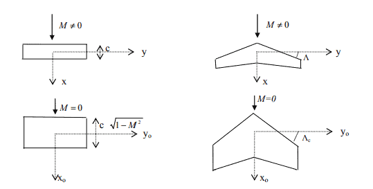
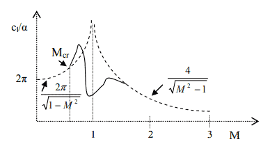
The evaluation methods for the sectional as well as the total lift and moment coefficients for unsteady subsonic and supersonic flows will be given in Chap. 5. It is, however, possible to obtain approximate expressions for the amplitude of the sectional lift coefficients at high reduced frequencies and at transonic regimes where M approaches to unity as limiting value. For steady flow on the other hand, the analytical expression is not readily available since the equations are nonlinear. However, local linearization process is applied to obtain approximate values for the aerodynamic coefficients.

Now, we can give the expression for the amplitude of the sectional lift coefficient for a simple harmonically pitching thin airfoil in transonic flow,
$$
\bar{c}_l \approx 4(1+i k) \bar{\alpha}, \quad k>1
$$
Here, $\bar{\alpha}$ is the amplitude of the angle of attack. Let us consider the same airfoil in a vertical motion with amplitude of $\bar{h}$.
$$
\bar{c}_l \approx 8 i k \bar{h} / b, \quad k>1
$$
All these formulae are available from (Bisplinghoff et al. 1996).
Aerodynamic response to the arbitrary motion of a thin airfoil in transonic flow will be studied in Chap. 5 with aid of relevant unit response function in different Mach numbers.

物理代写|空气动力学代写Aerodynamics代考|Slender Body Aerodynamics

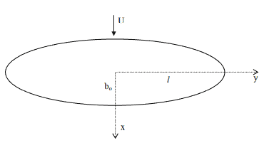
Munk-Jones airship theory is a good old useful tool for analyzing the aerodynamic behavior of slender bodies at small angles of attack even at supersonic speeds. The cross flow of a slender wing at a small angle of attack is approximately incompressible. Therefore, according to the Newton’s second law of motion, during the vertical motion of a slender body, the vertical momentum change of the air parcel with constant density displaced by the body motion is equal to the differential force acting on the body. Using this relation, we can decide on the aerodynamic stability of the slender body if we examine the sign of the aerodynamic moment about the center of gravity of the body. Expressing the change of the vertical force L, as a lifting force in terms of the cross sectional are $S$ and the equation of the axis $z=z_{\mathrm{a}}(x)$ of the body we obtain the following relation
$$
\frac{d L}{d x}=-\rho U^2 \frac{d}{d x}\left(S \frac{d z_a}{d x}\right)
$$
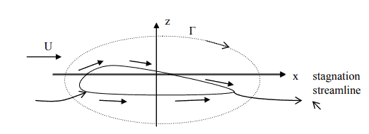
In Fig. 1.7, shown are the vertical forces affecting the slender body whose axis is at an angle of attack $\alpha$ with the free stream direction. Note that the vertical forces are non zero only at the nose and at the tail area because of the cross sectional area increase in those regions. Since there is no area change along the middle portion of the body, there is no vertical force generated at that portion of the body.

As we see in Fig. 1.7, the change of the moment with angle of attack taken around the center of gravity determines the stability of the body. The net moment of the forces acting at the nose and at the tail of the body counteracts with each other to give the sign of the total moment change with $\alpha$. The area increase at the tail section contributes to the stability as opposed to the apparent area increase at the nose region.

物理代写|空气动力学代写Aerodynamics代考|AES3530

空气动力学代考

物理代写|空气动力学代写空气动力学代考|可压缩非定常空气动力学


对于非定常亚音速和超声速流动,截面系数和总升力系数和力矩系数的计算方法将在第五章给出。然而,在M趋近于单位作为极限值的高降低频率和跨声速状态下,可以得到截面升力系数幅值的近似表达式。另一方面,对于定常流,由于方程是非线性的,解析表达式是不容易得到的。但是,采用局部线性化处理得到了气动系数的近似值


现在,我们可以给出跨声速流动中简单谐波俯仰薄翼型截面升力系数的幅值表达式,$$
\bar{c}_l \approx 4(1+i k) \bar{\alpha}, \quad k>1
$$
这里,$\bar{\alpha}$是迎角的幅值。让我们考虑同一翼型的垂直运动,振幅为$\bar{h}$ .
$$
\bar{c}_l \approx 8 i k \bar{h} / b, \quad k>1
$$
所有这些公式都可从(Bisplinghoff et al. 1996)。第五章将借助不同马赫数下的相关单位响应函数,研究薄翼型在跨音速流动中任意运动的气动响应

物理代写|空气动力学代写空气动力学代考|细长体空气动力学


Munk-Jones飞艇理论是一个古老而有用的工具,用于分析细长物体在小迎角下的气动行为,甚至在超音速。细长翼在小迎角时的横流几乎是不可压缩的。因此,根据牛顿第二运动定律,在细长体的垂直运动过程中,密度恒定的空气块被物体运动所移位的垂直动量变化等于作用在物体上的微分力。利用这一关系式,考察细长体重心的气动力矩符号,就可以确定细长体的气动稳定性。将垂直力L的变化表示为横截面的升力$S$和体轴$z=z_{\mathrm{a}}(x)$的方程,我们得到如下关系
$$
\frac{d L}{d x}=-\rho U^2 \frac{d}{d x}\left(S \frac{d z_a}{d x}\right)
$$
图1.7所示为影响细长体的垂直力,其轴与自由水流方向成迎角$\alpha$。注意,垂直力只有在机头和机尾区域不为零,因为这些区域的横截面积增加了。由于身体中间部分的面积没有变化,所以在身体的这部分不会产生垂直力


如图1.7所示,力矩随重心攻角的变化决定了物体的稳定性。作用在身体鼻子和尾部的力的净力矩相互抵消,给出总力矩变化的符号$\alpha$。与机头区域的表观面积增加相反,尾部区域的面积增加有助于稳定性

物理代写|空气动力学代写Aerodynamics代考 请认准statistics-lab™

统计代写请认准statistics-lab™. statistics-lab™为您的留学生涯保驾护航。

金融工程代写

金融工程是使用数学技术来解决金融问题。金融工程使用计算机科学、统计学、经济学和应用数学领域的工具和知识来解决当前的金融问题,以及设计新的和创新的金融产品。

非参数统计代写

非参数统计指的是一种统计方法,其中不假设数据来自于由少数参数决定的规定模型;这种模型的例子包括正态分布模型和线性回归模型。

广义线性模型代考

广义线性模型(GLM)归属统计学领域,是一种应用灵活的线性回归模型。该模型允许因变量的偏差分布有除了正态分布之外的其它分布。

术语 广义线性模型(GLM)通常是指给定连续和/或分类预测因素的连续响应变量的常规线性回归模型。它包括多元线性回归,以及方差分析和方差分析(仅含固定效应)。

有限元方法代写

有限元方法(FEM)是一种流行的方法,用于数值解决工程和数学建模中出现的微分方程。典型的问题领域包括结构分析、传热、流体流动、质量运输和电磁势等传统领域。

有限元是一种通用的数值方法,用于解决两个或三个空间变量的偏微分方程(即一些边界值问题)。为了解决一个问题,有限元将一个大系统细分为更小、更简单的部分,称为有限元。这是通过在空间维度上的特定空间离散化来实现的,它是通过构建对象的网格来实现的:用于求解的数值域,它有有限数量的点。边界值问题的有限元方法表述最终导致一个代数方程组。该方法在域上对未知函数进行逼近。[1] 然后将模拟这些有限元的简单方程组合成一个更大的方程系统,以模拟整个问题。然后,有限元通过变化微积分使相关的误差函数最小化来逼近一个解决方案。

tatistics-lab作为专业的留学生服务机构,多年来已为美国、英国、加拿大、澳洲等留学热门地的学生提供专业的学术服务,包括但不限于Essay代写,Assignment代写,Dissertation代写,Report代写,小组作业代写,Proposal代写,Paper代写,Presentation代写,计算机作业代写,论文修改和润色,网课代做,exam代考等等。写作范围涵盖高中,本科,研究生等海外留学全阶段,辐射金融,经济学,会计学,审计学,管理学等全球99%专业科目。写作团队既有专业英语母语作者,也有海外名校硕博留学生,每位写作老师都拥有过硬的语言能力,专业的学科背景和学术写作经验。我们承诺100%原创,100%专业,100%准时,100%满意。

随机分析代写


随机微积分是数学的一个分支,对随机过程进行操作。它允许为随机过程的积分定义一个关于随机过程的一致的积分理论。这个领域是由日本数学家伊藤清在第二次世界大战期间创建并开始的。

时间序列分析代写

随机过程,是依赖于参数的一组随机变量的全体,参数通常是时间。 随机变量是随机现象的数量表现,其时间序列是一组按照时间发生先后顺序进行排列的数据点序列。通常一组时间序列的时间间隔为一恒定值(如1秒,5分钟,12小时,7天,1年),因此时间序列可以作为离散时间数据进行分析处理。研究时间序列数据的意义在于现实中,往往需要研究某个事物其随时间发展变化的规律。这就需要通过研究该事物过去发展的历史记录,以得到其自身发展的规律。

回归分析代写

多元回归分析渐进(Multiple Regression Analysis Asymptotics)属于计量经济学领域,主要是一种数学上的统计分析方法,可以分析复杂情况下各影响因素的数学关系,在自然科学、社会和经济学等多个领域内应用广泛。

MATLAB代写

MATLAB 是一种用于技术计算的高性能语言。它将计算、可视化和编程集成在一个易于使用的环境中,其中问题和解决方案以熟悉的数学符号表示。典型用途包括:数学和计算算法开发建模、仿真和原型制作数据分析、探索和可视化科学和工程图形应用程序开发,包括图形用户界面构建MATLAB 是一个交互式系统,其基本数据元素是一个不需要维度的数组。这使您可以解决许多技术计算问题,尤其是那些具有矩阵和向量公式的问题,而只需用 C 或 Fortran 等标量非交互式语言编写程序所需的时间的一小部分。MATLAB 名称代表矩阵实验室。MATLAB 最初的编写目的是提供对由 LINPACK 和 EISPACK 项目开发的矩阵软件的轻松访问,这两个项目共同代表了矩阵计算软件的最新技术。MATLAB 经过多年的发展,得到了许多用户的投入。在大学环境中,它是数学、工程和科学入门和高级课程的标准教学工具。在工业领域,MATLAB 是高效研究、开发和分析的首选工具。MATLAB 具有一系列称为工具箱的特定于应用程序的解决方案。对于大多数 MATLAB 用户来说非常重要,工具箱允许您学习应用专业技术。工具箱是 MATLAB 函数(M 文件)的综合集合,可扩展 MATLAB 环境以解决特定类别的问题。可用工具箱的领域包括信号处理、控制系统、神经网络、模糊逻辑、小波、仿真等。

R语言代写问卷设计与分析代写
PYTHON代写回归分析与线性模型代写
MATLAB代写方差分析与试验设计代写
STATA代写机器学习/统计学习代写
SPSS代写计量经济学代写
EVIEWS代写时间序列分析代写
EXCEL代写深度学习代写
SQL代写各种数据建模与可视化代写

物理代写|空气动力学代写Aerodynamics代考|ASC4551

如果你也在 怎样代写空气动力学Aerodynamics这个学科遇到相关的难题,请随时右上角联系我们的24/7代写客服。

空气动力学是指空气在事物周围移动的方式。空气动力学的规则解释了飞机如何能够飞行。

statistics-lab™ 为您的留学生涯保驾护航 在代写空气动力学Aerodynamics方面已经树立了自己的口碑, 保证靠谱, 高质且原创的统计Statistics代写服务。我们的专家在代写空气动力学Aerodynamics代写方面经验极为丰富,各种代写空气动力学Aerodynamics相关的作业也就用不着说。

我们提供的空气动力学Aerodynamics及其相关学科的代写,服务范围广, 其中包括但不限于:

  • Statistical Inference 统计推断
  • Statistical Computing 统计计算
  • Advanced Probability Theory 高等概率论
  • Advanced Mathematical Statistics 高等数理统计学
  • (Generalized) Linear Models 广义线性模型
  • Statistical Machine Learning 统计机器学习
  • Longitudinal Data Analysis 纵向数据分析
  • Foundations of Data Science 数据科学基础
物理代写|空气动力学代写Aerodynamics代考|ASC4551

物理代写|空气动力学代写Aerodynamics代考|Steady Aerodynamics of Thin Wings

The finite wing aerodynamics, for special wing geometries, can yield analytical expressions for the aerodynamic coefficients in terms of the sectional properties of the wing. A special case is the elliptical span wise loading of the wing which is proportional to $\sqrt{l^2-y^2}$, where $\mathrm{y}$ is the span wise coordinate and 1 is the half span. For the wings with large span, using the Prandtl’s lifting line theory the wing’s lift coefficient $C_L$ becomes equal to the constant sectional lift coefficient $c_l$. Hence,
$$
C_L=c_l
$$
Another interesting aspect of the finite wing theory is the effect of the tip vortices on the overall performance of the wing. The tip vortices induce a vertical velocity which in turn induces additional drag on the wing. Hence, the total drag coefficient of the wing reads
$$
C_D=C_{D_o}+\frac{C_L^2}{\pi A R}
$$
Here the aspect ratio is $A R=l^2 / S$, and $\mathrm{S}$ is the wing area. For the symmetric and untwisted wings to have elliptical loading the plan form geometry also should be elliptical as shown in Fig. 1.3.

For the case of non-elliptical wings, we use the Glauert’s Fourier series expansion of the span wise variation of the circulation given by the lifting line theory. The integration of the numerically obtained span wise distribution of the circulation gives us the total lift coefficient.

If the aspect ratio of a wing is not so large and the sweep angle is larger than $15^{\circ}$, then we use the Weissenger’s L-Method to evaluate the lift coefficient of the wing.
For slender delta wings and for very low aspect ratio slender wings, analytical expressions for the lift and drag coefficients are also available. The lift coefficient for a delta wing without a camber in spanwise direction is
$$
C_L=\frac{1}{2} \pi A R \alpha
$$
The induced drag coefficient for delta wings having elliptical load distribution along their span is given as
$$
C_{D_i}=C_L \alpha / 2
$$

物理代写|空气动力学代写Aerodynamics代考|Compressible Steady Aerodynamics

It is a well known fact that at high speeds comparable with the speed of sound the effect of compressibility starts to play an important role on the aerodynamic characteristics of airfoil. At subsonic speeds, there exists a similarity between the compressible and incompressible external flows based on the Mach number $M=$ $U / a_{\infty}, a_{\infty}=$ free stream speed of sound. This similarity enables us to express the compressible pressure coefficient in terms of the incompressible pressure coefficient as follows
$$
c_p=\frac{c_{p_o}}{\sqrt{1-M^2}}
$$
Here,
$$
c_{p_o}=\frac{p_o-p_{\infty}}{\frac{1}{2} \rho_{\infty} U^2}
$$
is the surface pressure coefficient for the incompressible flow about a wing which is kept with a fixed thickness and span but stretched along the flow direction, $x$, with the following rule
$$
x_0=\frac{x}{\sqrt{1-M^2}}, y_0=y, z_0=z
$$
as shown in Fig. 1.4. The Prandtl-Glauert transformation for the wings is summarized by Eq. $1.14$ and Eq. $1.13$ is used to obtain the corresponding surface pressure coefficient. By this transformation, once we know the incompressible pressure coefficient at a point $x, y, z$, Eq. $1.13$ gives the pressure coefficient for the known free stream Mach number at the stretched coordinates $x_0, y_0, z_0$. As seen from Fig. 1.4, it is not practical to build a new plan form for each Mach number. Therefore, we need to find more practical approach in utilizing Prandtl-Glauert transformation.

For this purpose, assuming that the free stream density does not change for the both flows, we integrate Eq. $1.13$ in chord direction to obtain the same sectional lift coefficient for the incompressible and compressible flow. While doing so, if we keep the chord length same, i.e., divide $x_0$ with $\left(1-M^2\right)^{1 / 2}$, then the compressible sectional lift coefficient $c_1$ and moment coefficient $c_m$ become expressible in terms of the incompressible $c_{\mathrm{lo}}$ and $c_{\mathrm{mo}}$ as follows.

物理代写|空气动力学代写Aerodynamics代考|ASC4551

空气动力学代考

物理代写|空气动力学代写空气动力学代考|薄翼的稳定空气动力学


对于特殊的机翼几何形状,有限的机翼空气动力学可以根据机翼的截面特性得出气动系数的解析表达式。一种特殊情况是机翼的椭圆跨度加载,它与$\sqrt{l^2-y^2}$成正比,其中$\mathrm{y}$是跨度坐标,1是半跨度。对于大跨度机翼,根据普朗特升力线理论,机翼升力系数$C_L$等于常截面升力系数$c_l$。
$$
C_L=c_l
$$
有限翼理论另一个有趣的方面是翼尖涡对机翼整体性能的影响。翼尖涡产生垂直速度,进而对机翼产生额外阻力。因此,机翼的总阻力系数为
$$
C_D=C_{D_o}+\frac{C_L^2}{\pi A R}
$$
这里的纵横比是$A R=l^2 / S$, $\mathrm{S}$是机翼面积。为了使对称和未扭曲的机翼具有椭圆载荷,平面形状几何也应该是如图1.3所示的椭圆


对于非椭圆翼,我们使用了由升力线理论给出的循环的跨度变化的格劳埃特傅立叶级数展开。对得到的环流跨界分布的数值进行积分,得到总升力系数


如果机翼的展弦比不是那么大,而后掠角大于$15^{\circ}$,那么我们就用Weissenger’s L-Method来评估机翼的升力系数。对于细长三角翼和非常低展弦比细长翼,升力和阻力系数的解析表达式也可用。无弧度三角翼在展向方向的升力系数为
$$
C_L=\frac{1}{2} \pi A R \alpha
$$
而沿展向具有椭圆载荷分布的三角翼的诱导阻力系数为
$$
C_{D_i}=C_L \alpha / 2
$$

物理代写|空气动力学代写空气动力学代考|可压缩稳定空气动力学


众所周知,在与音速相当的高速下,可压缩性的影响开始对翼型的气动特性起重要作用。在亚声速下,基于马赫数$M=$$U / a_{\infty}, a_{\infty}=$自由声流速度的可压缩和不可压缩外部流之间存在相似性。这种相似性使我们可以用不可压缩压力系数表示可压缩压力系数如下:
$$
c_p=\frac{c_{p_o}}{\sqrt{1-M^2}}
$$
其中
$$
c_{p_o}=\frac{p_o-p_{\infty}}{\frac{1}{2} \rho_{\infty} U^2}
$$
是关于机翼不可压缩流动的表面压力系数,该机翼保持一定的厚度和跨度,但沿流动方向$x$拉伸,其规律如下:
$$
x_0=\frac{x}{\sqrt{1-M^2}}, y_0=y, z_0=z
$$
,如图1.4所示。机翼的Prandtl-Glauert变换由Eq. $1.14$和Eq. $1.13$总结,得到相应的表面压力系数。通过这种变换,一旦我们知道了$x, y, z$点的不可压缩压力系数,Eq. $1.13$就给出了已知自由流马赫数在拉伸坐标$x_0, y_0, z_0$处的压力系数。从图1.4可以看出,为每个马赫数建立一个新的平面形式是不实际的。因此,在利用Prandtl-Glauert变换时,我们需要寻找更实用的方法


为此,假设两种流的自由流密度不变,我们在弦向积分Eq. $1.13$,得到不可压缩流和可压缩流相同的截面升力系数。在此过程中,如果保持弦长不变,即$x_0$除以$\left(1-M^2\right)^{1 / 2}$,则可压缩截面升力系数$c_1$和弯矩系数$c_m$可用不可压缩截面$c_{\mathrm{lo}}$和$c_{\mathrm{mo}}$表示,如下:

物理代写|空气动力学代写Aerodynamics代考 请认准statistics-lab™

统计代写请认准statistics-lab™. statistics-lab™为您的留学生涯保驾护航。

金融工程代写

金融工程是使用数学技术来解决金融问题。金融工程使用计算机科学、统计学、经济学和应用数学领域的工具和知识来解决当前的金融问题,以及设计新的和创新的金融产品。

非参数统计代写

非参数统计指的是一种统计方法,其中不假设数据来自于由少数参数决定的规定模型;这种模型的例子包括正态分布模型和线性回归模型。

广义线性模型代考

广义线性模型(GLM)归属统计学领域,是一种应用灵活的线性回归模型。该模型允许因变量的偏差分布有除了正态分布之外的其它分布。

术语 广义线性模型(GLM)通常是指给定连续和/或分类预测因素的连续响应变量的常规线性回归模型。它包括多元线性回归,以及方差分析和方差分析(仅含固定效应)。

有限元方法代写

有限元方法(FEM)是一种流行的方法,用于数值解决工程和数学建模中出现的微分方程。典型的问题领域包括结构分析、传热、流体流动、质量运输和电磁势等传统领域。

有限元是一种通用的数值方法,用于解决两个或三个空间变量的偏微分方程(即一些边界值问题)。为了解决一个问题,有限元将一个大系统细分为更小、更简单的部分,称为有限元。这是通过在空间维度上的特定空间离散化来实现的,它是通过构建对象的网格来实现的:用于求解的数值域,它有有限数量的点。边界值问题的有限元方法表述最终导致一个代数方程组。该方法在域上对未知函数进行逼近。[1] 然后将模拟这些有限元的简单方程组合成一个更大的方程系统,以模拟整个问题。然后,有限元通过变化微积分使相关的误差函数最小化来逼近一个解决方案。

tatistics-lab作为专业的留学生服务机构,多年来已为美国、英国、加拿大、澳洲等留学热门地的学生提供专业的学术服务,包括但不限于Essay代写,Assignment代写,Dissertation代写,Report代写,小组作业代写,Proposal代写,Paper代写,Presentation代写,计算机作业代写,论文修改和润色,网课代做,exam代考等等。写作范围涵盖高中,本科,研究生等海外留学全阶段,辐射金融,经济学,会计学,审计学,管理学等全球99%专业科目。写作团队既有专业英语母语作者,也有海外名校硕博留学生,每位写作老师都拥有过硬的语言能力,专业的学科背景和学术写作经验。我们承诺100%原创,100%专业,100%准时,100%满意。

随机分析代写


随机微积分是数学的一个分支,对随机过程进行操作。它允许为随机过程的积分定义一个关于随机过程的一致的积分理论。这个领域是由日本数学家伊藤清在第二次世界大战期间创建并开始的。

时间序列分析代写

随机过程,是依赖于参数的一组随机变量的全体,参数通常是时间。 随机变量是随机现象的数量表现,其时间序列是一组按照时间发生先后顺序进行排列的数据点序列。通常一组时间序列的时间间隔为一恒定值(如1秒,5分钟,12小时,7天,1年),因此时间序列可以作为离散时间数据进行分析处理。研究时间序列数据的意义在于现实中,往往需要研究某个事物其随时间发展变化的规律。这就需要通过研究该事物过去发展的历史记录,以得到其自身发展的规律。

回归分析代写

多元回归分析渐进(Multiple Regression Analysis Asymptotics)属于计量经济学领域,主要是一种数学上的统计分析方法,可以分析复杂情况下各影响因素的数学关系,在自然科学、社会和经济学等多个领域内应用广泛。

MATLAB代写

MATLAB 是一种用于技术计算的高性能语言。它将计算、可视化和编程集成在一个易于使用的环境中,其中问题和解决方案以熟悉的数学符号表示。典型用途包括:数学和计算算法开发建模、仿真和原型制作数据分析、探索和可视化科学和工程图形应用程序开发,包括图形用户界面构建MATLAB 是一个交互式系统,其基本数据元素是一个不需要维度的数组。这使您可以解决许多技术计算问题,尤其是那些具有矩阵和向量公式的问题,而只需用 C 或 Fortran 等标量非交互式语言编写程序所需的时间的一小部分。MATLAB 名称代表矩阵实验室。MATLAB 最初的编写目的是提供对由 LINPACK 和 EISPACK 项目开发的矩阵软件的轻松访问,这两个项目共同代表了矩阵计算软件的最新技术。MATLAB 经过多年的发展,得到了许多用户的投入。在大学环境中,它是数学、工程和科学入门和高级课程的标准教学工具。在工业领域,MATLAB 是高效研究、开发和分析的首选工具。MATLAB 具有一系列称为工具箱的特定于应用程序的解决方案。对于大多数 MATLAB 用户来说非常重要,工具箱允许您学习应用专业技术。工具箱是 MATLAB 函数(M 文件)的综合集合,可扩展 MATLAB 环境以解决特定类别的问题。可用工具箱的领域包括信号处理、控制系统、神经网络、模糊逻辑、小波、仿真等。

R语言代写问卷设计与分析代写
PYTHON代写回归分析与线性模型代写
MATLAB代写方差分析与试验设计代写
STATA代写机器学习/统计学习代写
SPSS代写计量经济学代写
EVIEWS代写时间序列分析代写
EXCEL代写深度学习代写
SQL代写各种数据建模与可视化代写

物理代写|空气动力学代写Aerodynamics代考|ME471

如果你也在 怎样代写空气动力学Aerodynamics这个学科遇到相关的难题,请随时右上角联系我们的24/7代写客服。

空气动力学是指空气在事物周围移动的方式。空气动力学的规则解释了飞机如何能够飞行。

statistics-lab™ 为您的留学生涯保驾护航 在代写空气动力学Aerodynamics方面已经树立了自己的口碑, 保证靠谱, 高质且原创的统计Statistics代写服务。我们的专家在代写空气动力学Aerodynamics代写方面经验极为丰富,各种代写空气动力学Aerodynamics相关的作业也就用不着说。

我们提供的空气动力学Aerodynamics及其相关学科的代写,服务范围广, 其中包括但不限于:

  • Statistical Inference 统计推断
  • Statistical Computing 统计计算
  • Advanced Probability Theory 高等概率论
  • Advanced Mathematical Statistics 高等数理统计学
  • (Generalized) Linear Models 广义线性模型
  • Statistical Machine Learning 统计机器学习
  • Longitudinal Data Analysis 纵向数据分析
  • Foundations of Data Science 数据科学基础
物理代写|空气动力学代写Aerodynamics代考|ME471

物理代写|空气动力学代写Aerodynamics代考|Generation of Lift

The very basic theory of aerodynamics lies in the Kutta-Joukowski theorem. This theorem states that for an airfoil with round leading and sharp trailing edge immersed in a uniform stream with an effective angle of attack, there exists a lifting force proportional to the density of air $\rho$, free stream velocity $U$ and the circulation $\Gamma$ generated by the bound vortex. Hence, the sectional lifting force $l$ is equal to
$$
l=\rho U \Gamma
$$
Figure $1.1$ depicts the pertinent quantities involved in generation of lift.

The strength of the bound vortex is given by the circulation around the airfoil, $\Gamma=\oint \mathbf{V} . \mathbf{d s} .$

If the effective angle of attack is $\alpha$, and the chord length of the airfoil is $c=2 b$, with the Ionkowski transformation the magnitude of the circulation is found as $\Gamma=2 \pi \alpha \mathrm{b} U$. Substituting the value of $\Gamma$ into Eq. $1.1$ gives the sectional lift force as
$$
l=2 \rho \pi \alpha b U^2
$$
Using the definition of sectional lift coefficient for the steady flow we obtain,
$$
c_l=\frac{l}{\rho U^2 b}=2 \pi \alpha
$$
The very same result can be obtained by integrating the relation between the vortex sheet strength $\gamma_{\mathrm{a}}$ and the lifting surface pressure coefficient $\mathrm{c}{\mathrm{pa}}$ along the chord as follows. $$ \mathrm{c}{\mathrm{pa}}(x)=\mathrm{c}{\mathrm{pl}}-\mathrm{c}{\mathrm{pu}}=2 \gamma_{\mathrm{a}}(x) / \mathrm{U}
$$
The lifting presssure coéfficient for an aairfoil with angle of attack reads as
$$
c_{p a}(x)=2 \alpha \sqrt{\frac{b-x}{b+x}}, \quad-b \leq x \leq b
$$

物理代写|空气动力学代写Aerodynamics代考|Unsteady Lifting Force Coefficient

During rapidly changing unsteady motion of an airfoil the aerodynamic response is no longer the timewise slightly changing steady phenomenon.

For example, let us consider a thin airfoil with a chord length of $2 \mathrm{~b}$ undergoing a vertical simple harmonic motion in a free stream of $U$ with zero angle of attack. If the amplitude of the vertical motion is $\bar{h}$ and the angular frequency is $\omega$ then the profile location at any lime $t$ reads as
$$
z_a(t)=\bar{h} e^{i \omega t}
$$
If we implement the pure steady aerodynamics approach, because of Eq. $1.3$ the sectional lift coefficient will read as zero. Now, we write the time dependent sectional lift coefficient in terms of the reduced frequency $k=\omega \mathrm{b} / \mathrm{U}$ and the non-dimensional amplitude $\bar{h}^=\bar{h} / b$. $$ c_l(t)=\left[-2 i k C(k) \bar{h}^+k^2 \bar{h}^\right] \pi e^{i \omega t} $$ Let us now analyze each term in Eq. $1.6$ in terms of the relevant aerodynamics. (i) Unsteady Aerodynamics: If we consider all the terms in Eq. $1.6$ then the analysis is based on unsteady aerodynamics. $C(k)$ in the first term of the expression is a complex function and called the Theodorsen function which is the measure of the phase lag between the motion and aerodynamic response. The second term, on the other hand, is the acceleration term based on the inertia of the air parcel displaced during the motion. It is called the apparent mass term and is significant for the reduced frequency values larger than unity. (ii) Quasi Unsteady Aerodynamics: If we neglect the apparent mass term in Eq. 1.6 the aerodynamic analysis is then called quasi unsteady aerodynamics. Accordingly, the sectional lift coefficient reads as $$ c_l(t)=\left[-2 \pi i k C(k) \bar{h}^\right] e^{i \omega t}
$$

物理代写|空气动力学代写Aerodynamics代考|ME471

空气动力学代考

物理代写|空气动力学代写空气动力学代考|产生升力


空气动力学最基本的理论是库塔-朱可夫斯基定理。该定理指出,当前缘圆后缘尖的翼型浸没在具有有效迎角的均匀气流中时,存在与空气密度$\rho$、自由气流速度$U$和束缚涡产生的循环$\Gamma$成正比的升力。因此,截面升力$l$等于
$$
l=\rho U \Gamma
$$
图$1.1$描述了产生升力的相关量。


结合涡旋的强度是由翼型周围的环流给出的,$\Gamma=\oint \mathbf{V} . \mathbf{d s} .$


如果有效迎角为$\alpha$,翼型的弦长为$c=2 b$,通过Ionkowski变换得到环流的大小为$\Gamma=2 \pi \alpha \mathrm{b} U$。将$\Gamma$的值代入Eq. $1.1$,则截面升力为
$$
l=2 \rho \pi \alpha b U^2
$$
根据我们得到的稳态流动的截面升力系数的定义,
$$
c_l=\frac{l}{\rho U^2 b}=2 \pi \alpha
$$
将涡旋片强度$\gamma_{\mathrm{a}}$与沿chord升力面压力系数$\mathrm{c}{\mathrm{pa}}$之间的关系积分,也可以得到同样的结果。$$ \mathrm{c}{\mathrm{pa}}(x)=\mathrm{c}{\mathrm{pl}}-\mathrm{c}{\mathrm{pu}}=2 \gamma_{\mathrm{a}}(x) / \mathrm{U}
$$
提升压力coéfficient为一个迎角翼型读为
$$
c_{p a}(x)=2 \alpha \sqrt{\frac{b-x}{b+x}}, \quad-b \leq x \leq b
$$

物理代写|空气动力学代写空气动力学代考|非定常升力系数


在翼型快速变化的非定常运动过程中,气动响应不再是按时间顺序的微小变化的稳态现象


例如,让我们考虑一个弦长为$2 \mathrm{~b}$的薄翼型,以零迎角在$U$的自由流中进行垂直简谐运动。如果垂直运动的振幅是$\bar{h}$,角频率是$\omega$,那么在任何位置$t$处的剖面位置读起来都是
$$
z_a(t)=\bar{h} e^{i \omega t}
$$
如果我们采用纯稳定空气动力学方法,由于Eq. $1.3$,截面升力系数将读起来是零。现在,我们用减少的频率$k=\omega \mathrm{b} / \mathrm{U}$和无维振幅$\bar{h}^=\bar{h} / b$来表示与时间相关的截面升力系数。$$ c_l(t)=\left[-2 i k C(k) \bar{h}^+k^2 \bar{h}^\right] \pi e^{i \omega t} $$现在让我们从相关的空气动力学角度来分析Eq. $1.6$中的每一项。(i)非定常空气动力学:如果我们考虑Eq. $1.6$中的所有术语,那么分析是基于非定常空气动力学的。$C(k)$在表达式的第一项是一个复函数,称为Theodorsen函数,它是运动和气动响应之间相位滞后的度量。第二项,另一方面,是加速度项基于运动中移位的空气块的惯性。它被称为表观质量项,对于大于单位的频率值的减少是有意义的。(ii)准非定常空气动力学:如果忽略式1.6中的表观质量项,则气动分析称为准非定常空气动力学。因此,截面升力系数为$$ c_l(t)=\left[-2 \pi i k C(k) \bar{h}^\right] e^{i \omega t}
$$

物理代写|空气动力学代写Aerodynamics代考 请认准statistics-lab™

统计代写请认准statistics-lab™. statistics-lab™为您的留学生涯保驾护航。

金融工程代写

金融工程是使用数学技术来解决金融问题。金融工程使用计算机科学、统计学、经济学和应用数学领域的工具和知识来解决当前的金融问题,以及设计新的和创新的金融产品。

非参数统计代写

非参数统计指的是一种统计方法,其中不假设数据来自于由少数参数决定的规定模型;这种模型的例子包括正态分布模型和线性回归模型。

广义线性模型代考

广义线性模型(GLM)归属统计学领域,是一种应用灵活的线性回归模型。该模型允许因变量的偏差分布有除了正态分布之外的其它分布。

术语 广义线性模型(GLM)通常是指给定连续和/或分类预测因素的连续响应变量的常规线性回归模型。它包括多元线性回归,以及方差分析和方差分析(仅含固定效应)。

有限元方法代写

有限元方法(FEM)是一种流行的方法,用于数值解决工程和数学建模中出现的微分方程。典型的问题领域包括结构分析、传热、流体流动、质量运输和电磁势等传统领域。

有限元是一种通用的数值方法,用于解决两个或三个空间变量的偏微分方程(即一些边界值问题)。为了解决一个问题,有限元将一个大系统细分为更小、更简单的部分,称为有限元。这是通过在空间维度上的特定空间离散化来实现的,它是通过构建对象的网格来实现的:用于求解的数值域,它有有限数量的点。边界值问题的有限元方法表述最终导致一个代数方程组。该方法在域上对未知函数进行逼近。[1] 然后将模拟这些有限元的简单方程组合成一个更大的方程系统,以模拟整个问题。然后,有限元通过变化微积分使相关的误差函数最小化来逼近一个解决方案。

tatistics-lab作为专业的留学生服务机构,多年来已为美国、英国、加拿大、澳洲等留学热门地的学生提供专业的学术服务,包括但不限于Essay代写,Assignment代写,Dissertation代写,Report代写,小组作业代写,Proposal代写,Paper代写,Presentation代写,计算机作业代写,论文修改和润色,网课代做,exam代考等等。写作范围涵盖高中,本科,研究生等海外留学全阶段,辐射金融,经济学,会计学,审计学,管理学等全球99%专业科目。写作团队既有专业英语母语作者,也有海外名校硕博留学生,每位写作老师都拥有过硬的语言能力,专业的学科背景和学术写作经验。我们承诺100%原创,100%专业,100%准时,100%满意。

随机分析代写


随机微积分是数学的一个分支,对随机过程进行操作。它允许为随机过程的积分定义一个关于随机过程的一致的积分理论。这个领域是由日本数学家伊藤清在第二次世界大战期间创建并开始的。

时间序列分析代写

随机过程,是依赖于参数的一组随机变量的全体,参数通常是时间。 随机变量是随机现象的数量表现,其时间序列是一组按照时间发生先后顺序进行排列的数据点序列。通常一组时间序列的时间间隔为一恒定值(如1秒,5分钟,12小时,7天,1年),因此时间序列可以作为离散时间数据进行分析处理。研究时间序列数据的意义在于现实中,往往需要研究某个事物其随时间发展变化的规律。这就需要通过研究该事物过去发展的历史记录,以得到其自身发展的规律。

回归分析代写

多元回归分析渐进(Multiple Regression Analysis Asymptotics)属于计量经济学领域,主要是一种数学上的统计分析方法,可以分析复杂情况下各影响因素的数学关系,在自然科学、社会和经济学等多个领域内应用广泛。

MATLAB代写

MATLAB 是一种用于技术计算的高性能语言。它将计算、可视化和编程集成在一个易于使用的环境中,其中问题和解决方案以熟悉的数学符号表示。典型用途包括:数学和计算算法开发建模、仿真和原型制作数据分析、探索和可视化科学和工程图形应用程序开发,包括图形用户界面构建MATLAB 是一个交互式系统,其基本数据元素是一个不需要维度的数组。这使您可以解决许多技术计算问题,尤其是那些具有矩阵和向量公式的问题,而只需用 C 或 Fortran 等标量非交互式语言编写程序所需的时间的一小部分。MATLAB 名称代表矩阵实验室。MATLAB 最初的编写目的是提供对由 LINPACK 和 EISPACK 项目开发的矩阵软件的轻松访问,这两个项目共同代表了矩阵计算软件的最新技术。MATLAB 经过多年的发展,得到了许多用户的投入。在大学环境中,它是数学、工程和科学入门和高级课程的标准教学工具。在工业领域,MATLAB 是高效研究、开发和分析的首选工具。MATLAB 具有一系列称为工具箱的特定于应用程序的解决方案。对于大多数 MATLAB 用户来说非常重要,工具箱允许您学习应用专业技术。工具箱是 MATLAB 函数(M 文件)的综合集合,可扩展 MATLAB 环境以解决特定类别的问题。可用工具箱的领域包括信号处理、控制系统、神经网络、模糊逻辑、小波、仿真等。

R语言代写问卷设计与分析代写
PYTHON代写回归分析与线性模型代写
MATLAB代写方差分析与试验设计代写
STATA代写机器学习/统计学习代写
SPSS代写计量经济学代写
EVIEWS代写时间序列分析代写
EXCEL代写深度学习代写
SQL代写各种数据建模与可视化代写

物理代写|空气动力学代写Aerodynamics代考|AOE4124

如果你也在 怎样代写空气动力学Aerodynamics这个学科遇到相关的难题,请随时右上角联系我们的24/7代写客服。

空气动力学是对空气运动的研究,特别是当受到固体物体,如飞机机翼影响时。

statistics-lab™ 为您的留学生涯保驾护航 在代写空气动力学Aerodynamics方面已经树立了自己的口碑, 保证靠谱, 高质且原创的统计Statistics代写服务。我们的专家在代写空气动力学Aerodynamics代写方面经验极为丰富,各种代写空气动力学Aerodynamics相关的作业也就用不着说。

我们提供的空气动力学Aerodynamics及其相关学科的代写,服务范围广, 其中包括但不限于:

  • Statistical Inference 统计推断
  • Statistical Computing 统计计算
  • Advanced Probability Theory 高等概率论
  • Advanced Mathematical Statistics 高等数理统计学
  • (Generalized) Linear Models 广义线性模型
  • Statistical Machine Learning 统计机器学习
  • Longitudinal Data Analysis 纵向数据分析
  • Foundations of Data Science 数据科学基础
物理代写|空气动力学代写Aerodynamics代考|AOE4124

物理代写|空气动力学代写Aerodynamics代考|Mathematical Models of Fluid Flow

The Navier-Stokes equations state the laws of conservation of mass, momentum, and energy for the flow of a gas in thermodynamic equilibrium. Using the Cartesian tensor notation, let $x_i$ be the coordinates; $p, \rho, T, E$, and $H$ the pressure, density, temperature, and total energy and enthalpy; and $u_i$ the velocity components, where for three-dimensional flow $i$ ranges from 1 to 3 . Also, we use the summation convention that a repeated index implies a sum over that index. Each conservation equation has the differential form
$$
\frac{\partial w}{\partial t}+\frac{\partial f_j}{\partial x_j}=0,
$$
which can be derived from the integral form
$$
\frac{\partial}{\partial t} \int_D w d V+\int_B f_j n_j d S=0,
$$
for a control volume $D$ with boundary $B$, where $d V$ and $d S$ are the volume and area elements, and $n_j$ are the components of the surface normal. The integral form remains valid in the presence of discontinuities such as shock waves and is the basis of the finite volume method, which is discussed in detail in subsequent chapters. For the mass equation,
$$
w=p, \quad f_j=\rho u_j .
$$
For the $i$ momentum equation,
$$
w_i=\rho u_i, \quad f_{i j}=\rho u_i u_j+p \delta_{i j}-\tau_{i j},
$$
where $\tau_{i j}$ is the viscous stress tensor, which for a Newtonian fluid is proportional to the rate of strain tensor and the bulk dilatation, and $\delta_{i j}$ is the Kronecker delta
$$
\delta_{i j}=\left{\begin{array}{lll}
1 & \text { if } \quad i=j \
0 & \text { if } \quad i \neq j
\end{array} .\right.
$$
If $\mu$ and $\lambda$ are the coefficients of viscosity and bulk viscosity, then
$$
\tau_{i j}=\mu\left(\frac{\partial u_i}{\partial x_j}+\frac{\partial u_j}{\partial x_i}\right)+\lambda \delta_{i j}\left(\frac{\partial u_k}{\partial x_k}\right) .
$$

物理代写|空气动力学代写Aerodynamics代考|Coordinate Transformations

In order to calculate solutions for flows in complex geometric domains, it is often useful to introduce body-fitted coordinates through global or, as in the case of isoparametric elements, local transformations. With the body now coinciding with a coordinate surface, it is much easier to enforce the boundary conditions accurately. Suppose that the mapping to computational coordinates $\left(\varepsilon_1, \varepsilon_2, \varepsilon_3\right)$ is defined by the transformation matrices
$$
K_{i j}=\frac{\partial x_i}{\partial \xi_j}, \quad K_{i j}^{-1}=\frac{\partial \xi_i}{\partial x_j}, \quad J=\operatorname{det}(K)
$$
where for the sake of simplicity it is assumed that $K$ and $J$ are independent of time.
Also define
$$
S=J K^{-1}
$$
The elements of $S$ are the cofactors of $K$, and in a finite volume discretization, they are just the face areas of the computational cells projected in the $x_1, x_2$, and $x_3$ directions. Using the Levi-Civita permutation symbol
$$
\epsilon_{i j k}= \begin{cases}+1 & \text { if } \quad(i, j, k) \text { is }(1,2,3),(2,3,1), \text { or }(3,1,2) \ -1 & \text { if }(i, j, k) \text { is }(3,2,1),(1,3,2), \text { or }(2,1,3), \ 0 & \text { if } i=j \quad \text { or } j=k \quad \text { or } \quad k=i\end{cases}
$$
we can express the elements of $S$ as
$$
S_{i j}=\frac{1}{2} \epsilon_{j p q} \epsilon_{i r s} \frac{\partial x_p}{\partial \xi_r} \frac{\partial x_q}{\partial \xi_s} .
$$

物理代写|空气动力学代写Aerodynamics代考|AOE4124

空气动力学代考

物理代写|空气动力学代写空气动力学代考|流体流动数学模型


Navier-Stokes方程描述了气体在热力学平衡中流动的质量、动量和能量守恒定律。利用笛卡尔张量符号,让 $x_i$ 是坐标; $p, \rho, T, E$,以及 $H$ 压强,密度,温度,总能量和焓;和 $u_i$ 速度分量,这里是三维流动 $i$ 取值范围为1 ~ 3。此外,我们使用求和约定,重复索引意味着对该索引的和。每个守恒方程都有微分形式
$$
\frac{\partial w}{\partial t}+\frac{\partial f_j}{\partial x_j}=0,
$$
,它可以由积分形式
导出$$
\frac{\partial}{\partial t} \int_D w d V+\int_B f_j n_j d S=0,
$$
为控制卷 $D$ 有边界 $B$,其中 $d V$ 和 $d S$ 体积和面积元素,和 $n_j$ 是曲面法线的分量。积分形式在诸如激波等不连续情况下仍然有效,是有限体积法的基础,我们将在后续章节详细讨论。对于质量方程,
$$
w=p, \quad f_j=\rho u_j .
$$
对于 $i$ 动量方程,
$$
w_i=\rho u_i, \quad f_{i j}=\rho u_i u_j+p \delta_{i j}-\tau_{i j},
$$
where $\tau_{i j}$ 为粘滞应力张量,对于牛顿流体,粘滞应力张量与应变张量的速率和体积膨胀率成正比,且 $\delta_{i j}$ 克罗内克函数是否
$$
\delta_{i j}=\left{\begin{array}{lll}
1 & \text { if } \quad i=j \
0 & \text { if } \quad i \neq j
\end{array} .\right.
$$
如果 $\mu$ 和 $\lambda$ 那么粘度系数和体粘度系数是否
$$
\tau_{i j}=\mu\left(\frac{\partial u_i}{\partial x_j}+\frac{\partial u_j}{\partial x_i}\right)+\lambda \delta_{i j}\left(\frac{\partial u_k}{\partial x_k}\right) .
$$

物理代写|空气动力学代写空气动力学代考|坐标转换


为了计算复杂几何域中流动的解,通常通过全局变换或如等参元素的情况下的局部变换引入拟合坐标是有用的。由于物体现在与一个坐标曲面重合,精确地执行边界条件就容易得多了。假设到计算坐标$\left(\varepsilon_1, \varepsilon_2, \varepsilon_3\right)$的映射由转换矩阵
$$
K_{i j}=\frac{\partial x_i}{\partial \xi_j}, \quad K_{i j}^{-1}=\frac{\partial \xi_i}{\partial x_j}, \quad J=\operatorname{det}(K)
$$
定义,其中为了简单起见,假设$K$和$J$与时间无关。
也定义
$$
S=J K^{-1}
$$
$S$的元素是$K$的余因子,并且在有限体积离散化中,它们只是计算单元在$x_1, x_2$和$x_3$方向上投影的面面积。使用Levi-Civita排列符号
$$
\epsilon_{i j k}= \begin{cases}+1 & \text { if } \quad(i, j, k) \text { is }(1,2,3),(2,3,1), \text { or }(3,1,2) \ -1 & \text { if }(i, j, k) \text { is }(3,2,1),(1,3,2), \text { or }(2,1,3), \ 0 & \text { if } i=j \quad \text { or } j=k \quad \text { or } \quad k=i\end{cases}
$$
,我们可以将$S$的元素表示为
$$
S_{i j}=\frac{1}{2} \epsilon_{j p q} \epsilon_{i r s} \frac{\partial x_p}{\partial \xi_r} \frac{\partial x_q}{\partial \xi_s} .
$$

物理代写|空气动力学代写Aerodynamics代考 请认准statistics-lab™

统计代写请认准statistics-lab™. statistics-lab™为您的留学生涯保驾护航。

金融工程代写

金融工程是使用数学技术来解决金融问题。金融工程使用计算机科学、统计学、经济学和应用数学领域的工具和知识来解决当前的金融问题,以及设计新的和创新的金融产品。

非参数统计代写

非参数统计指的是一种统计方法,其中不假设数据来自于由少数参数决定的规定模型;这种模型的例子包括正态分布模型和线性回归模型。

广义线性模型代考

广义线性模型(GLM)归属统计学领域,是一种应用灵活的线性回归模型。该模型允许因变量的偏差分布有除了正态分布之外的其它分布。

术语 广义线性模型(GLM)通常是指给定连续和/或分类预测因素的连续响应变量的常规线性回归模型。它包括多元线性回归,以及方差分析和方差分析(仅含固定效应)。

有限元方法代写

有限元方法(FEM)是一种流行的方法,用于数值解决工程和数学建模中出现的微分方程。典型的问题领域包括结构分析、传热、流体流动、质量运输和电磁势等传统领域。

有限元是一种通用的数值方法,用于解决两个或三个空间变量的偏微分方程(即一些边界值问题)。为了解决一个问题,有限元将一个大系统细分为更小、更简单的部分,称为有限元。这是通过在空间维度上的特定空间离散化来实现的,它是通过构建对象的网格来实现的:用于求解的数值域,它有有限数量的点。边界值问题的有限元方法表述最终导致一个代数方程组。该方法在域上对未知函数进行逼近。[1] 然后将模拟这些有限元的简单方程组合成一个更大的方程系统,以模拟整个问题。然后,有限元通过变化微积分使相关的误差函数最小化来逼近一个解决方案。

tatistics-lab作为专业的留学生服务机构,多年来已为美国、英国、加拿大、澳洲等留学热门地的学生提供专业的学术服务,包括但不限于Essay代写,Assignment代写,Dissertation代写,Report代写,小组作业代写,Proposal代写,Paper代写,Presentation代写,计算机作业代写,论文修改和润色,网课代做,exam代考等等。写作范围涵盖高中,本科,研究生等海外留学全阶段,辐射金融,经济学,会计学,审计学,管理学等全球99%专业科目。写作团队既有专业英语母语作者,也有海外名校硕博留学生,每位写作老师都拥有过硬的语言能力,专业的学科背景和学术写作经验。我们承诺100%原创,100%专业,100%准时,100%满意。

随机分析代写


随机微积分是数学的一个分支,对随机过程进行操作。它允许为随机过程的积分定义一个关于随机过程的一致的积分理论。这个领域是由日本数学家伊藤清在第二次世界大战期间创建并开始的。

时间序列分析代写

随机过程,是依赖于参数的一组随机变量的全体,参数通常是时间。 随机变量是随机现象的数量表现,其时间序列是一组按照时间发生先后顺序进行排列的数据点序列。通常一组时间序列的时间间隔为一恒定值(如1秒,5分钟,12小时,7天,1年),因此时间序列可以作为离散时间数据进行分析处理。研究时间序列数据的意义在于现实中,往往需要研究某个事物其随时间发展变化的规律。这就需要通过研究该事物过去发展的历史记录,以得到其自身发展的规律。

回归分析代写

多元回归分析渐进(Multiple Regression Analysis Asymptotics)属于计量经济学领域,主要是一种数学上的统计分析方法,可以分析复杂情况下各影响因素的数学关系,在自然科学、社会和经济学等多个领域内应用广泛。

MATLAB代写

MATLAB 是一种用于技术计算的高性能语言。它将计算、可视化和编程集成在一个易于使用的环境中,其中问题和解决方案以熟悉的数学符号表示。典型用途包括:数学和计算算法开发建模、仿真和原型制作数据分析、探索和可视化科学和工程图形应用程序开发,包括图形用户界面构建MATLAB 是一个交互式系统,其基本数据元素是一个不需要维度的数组。这使您可以解决许多技术计算问题,尤其是那些具有矩阵和向量公式的问题,而只需用 C 或 Fortran 等标量非交互式语言编写程序所需的时间的一小部分。MATLAB 名称代表矩阵实验室。MATLAB 最初的编写目的是提供对由 LINPACK 和 EISPACK 项目开发的矩阵软件的轻松访问,这两个项目共同代表了矩阵计算软件的最新技术。MATLAB 经过多年的发展,得到了许多用户的投入。在大学环境中,它是数学、工程和科学入门和高级课程的标准教学工具。在工业领域,MATLAB 是高效研究、开发和分析的首选工具。MATLAB 具有一系列称为工具箱的特定于应用程序的解决方案。对于大多数 MATLAB 用户来说非常重要,工具箱允许您学习应用专业技术。工具箱是 MATLAB 函数(M 文件)的综合集合,可扩展 MATLAB 环境以解决特定类别的问题。可用工具箱的领域包括信号处理、控制系统、神经网络、模糊逻辑、小波、仿真等。

R语言代写问卷设计与分析代写
PYTHON代写回归分析与线性模型代写
MATLAB代写方差分析与试验设计代写
STATA代写机器学习/统计学习代写
SPSS代写计量经济学代写
EVIEWS代写时间序列分析代写
EXCEL代写深度学习代写
SQL代写各种数据建模与可视化代写

物理代写|空气动力学代写Aerodynamics代考|ASC4551

如果你也在 怎样代写空气动力学Aerodynamics这个学科遇到相关的难题,请随时右上角联系我们的24/7代写客服。

空气动力学是对空气运动的研究,特别是当受到固体物体,如飞机机翼影响时。

statistics-lab™ 为您的留学生涯保驾护航 在代写空气动力学Aerodynamics方面已经树立了自己的口碑, 保证靠谱, 高质且原创的统计Statistics代写服务。我们的专家在代写空气动力学Aerodynamics代写方面经验极为丰富,各种代写空气动力学Aerodynamics相关的作业也就用不着说。

我们提供的空气动力学Aerodynamics及其相关学科的代写,服务范围广, 其中包括但不限于:

  • Statistical Inference 统计推断
  • Statistical Computing 统计计算
  • Advanced Probability Theory 高等概率论
  • Advanced Mathematical Statistics 高等数理统计学
  • (Generalized) Linear Models 广义线性模型
  • Statistical Machine Learning 统计机器学习
  • Longitudinal Data Analysis 纵向数据分析
  • Foundations of Data Science 数据科学基础
物理代写|空气动力学代写Aerodynamics代考|ASC4551

物理代写|空气动力学代写Aerodynamics代考|The Development of Methods for the Euler and Navier–Stokes Equations

By the $1980 \mathrm{~s}$, advances in computer hardware had made it feasible to solve the full Euler equations using software that could be cost-effective in industrial use. The idea of directly discretizing the conservation laws to produce a finite volume scheme had been introduced by MacCormack (MacCormack \& Paullay 1972). Most of the early flow solvers tended to exhibit strong pre- or post-shock oscillations. Also, in a workshop held in Stockholm in 1979 (Rizzi \& Viviand 1981), it was apparent that none of the existing schemes converged to a steady state. These difficulties were resolved during the following decade.

The Jameson-Schmidt-Turkel scheme (Jameson, Schmidt, \& Turkel 1981), which used Runge-Kutta time stepping and a blend of second- and fourth-differences (both to control oscillations and to provide background dissipation), consistently demonstrated convergence to a steady state, with the consequence that it has remained one of the most widely used methods to the present day.

A fairly complete understanding of shock capturing algorithms was achieved, stemming from the ideas of Godunov, Van Leer, Harten, and Roe. The issue of oscillation control and positivity had already been addressed by Godunov (1959) in his pioneering work in the 1950s (translated into English in 1959). He had introduced the concept of representing the flow as piecewise constant in each computational cell and solving a Riemann problem at each interface, thus obtaining a first order accurate solution that avoids nonphysical features such as expansion shocks. When this work was eventually recognized in the West, it became very influential. It was also widely recognized that numerical schemes might benefit from distinguishing the various wave speeds, and this motivated the development of characteristics-based schemes.

The earliest higher order characteristics-based methods used flux vector splitting (Steger \& Warming 1981) but suffered from oscillations near discontinuities similar to those of central difference schemes in the absence of numerical dissipation. The Monotone Upwind Scheme for Conservation Laws (MUSCL) of Van Leer (1974) extended the monotonicity-preserving behavior of Godunov’s scheme to higher order through the use of limiters. The use of limiters dates back to the fluxcorrected transport (FCT) scheme of Boris and Book (1973). A general framework for oscillation control in the solution of nonlinear problems was provided by Harten’s concept of Total Variation Diminishing (TVD) schemes. It finally proved possible to give a rigorous justification of the JST scheme (Jameson 1995a, 1995b).

物理代写|空气动力学代写Aerodynamics代考|Overview of the Simulation Process

The essential steps of developing a numerical simulation of a physical problem can be outlined as follows:

  1. Formulate a mathematical model of the physical problem that captures the important aspects for the purpose in hand and can provide the desired accuracy. Here it should be noted that models of widely varying complexity and levels of fidelity can be useful. For example, potential flow models based on Laplace’s equation can provide reasonably accurate predictions of low speed aerodynamic flows over streamlined shapes at a low computational cost, and this is very useful at an early stage in the design when rapid turnaround is crucial. At the final stage of the design, one would wish to confirm the expected performance using a model with the highest possible fidelity, typically the Reynolds averaged Navier-Stokes equations in actual practice.
  2. Analyze the mathematical properties of the model, such as proper formulation of boundary conditions that ensure the existence and convergence of a solution.
  3. Formulate a discrete numerical scheme to approximate the mathematical model that has been selected. Analyze the stability, accuracy, and convergence of the scheme. Can we prove, for example, that the error in the numerical approximation decreases as some power of the mesh spacing when the spacing is progressively reduced?
  4. Implement the discrete scheme in software that makes efficient use of the available hardware. This is becoming harder with the emergence of parallel systems with multiple levels of parallelism down to multiple threads within each core of multi-core processing chips, which are in turn arranged in parallel clusters. This stage also requires the use of every possible procedure to assure that the software is actually correct.
  5. Validate the software by showing that it produces trustworthy results in practice. Here we should distinguish between the questions of whether the software is correct and whether the selected mathematical model adequately represents the physics. To address the first question, we may test whether the results are correct for some limiting situations for which the true answer is known. For example, an arbitrary body has zero drag in inviscid flow. Or is the numerical solution symmetric for flow over a symmetric profile at zero angle of attack? We should also test the convergence of the numerical solution as the grid is refined. Does it exhibit the expected order of accuracy? We may also compare the results with those obtained by other software developed to solve the same problem. Workshops such as the AIAA Drag Prediction Workshops can play a useful role in this process. Finally, once a sufficiently high confidence level has been established for the software, comparisons with experimental data can be used to address the question of whether the mathematical model adequately represents the physical problem of interest.
物理代写|空气动力学代写Aerodynamics代考|ASC4551

空气动力学代考

物理代写|空气动力学代写空气动力学代考|欧拉和Navier-Stokes方程方法的发展


到$1980 \mathrm{~s}$时,计算机硬件的进步已使使用在工业上具有成本效益的软件解决完整的欧拉方程成为可能。将守恒律直接离散以产生有限体积格式的思想是由MacCormack (MacCormack &Paullay 1972)。大多数早期的流体求解器往往表现出强烈的冲击前后振荡。此外,在1979年斯德哥尔摩举行的研讨会上(Rizzi &Viviand 1981年),显然没有一个现有的方案收敛到稳定状态。这些困难在随后的十年中得到了解决

Jameson-Schmidt- turkel方案(Jameson, Schmidt, &Turkel 1981),它使用龙格-库塔时间步进和第二差分和第四差分的混合(用于控制振荡和提供背景耗散),一致证明了收敛到稳态,其结果是它一直是最广泛使用的方法之一直到今天


基于Godunov、Van Leer、Harten和Roe的思想,人们对冲击捕获算法有了相当完整的理解。振荡控制和正的问题已经被Godunov(1959)在他的开创性工作在20世纪50年代(1959年翻译成英语)。他引入了在每个计算单元中将流表示为分段常数的概念,并在每个接口上求解黎曼问题,从而获得一阶精确解,避免了膨胀冲击等非物理特征。当这项工作最终在西方得到认可时,它变得非常有影响力。人们也普遍认识到,数值格式可能受益于区分不同的波速,这推动了基于特征的格式的发展


最早的高阶基于特征的方法使用通量矢量分裂(Steger &但在没有数值耗散的情况下,与中心差分格式的振荡相似,在不连续附近产生振荡。Van Leer(1974)的守恒定律单调逆风格式(MUSCL)通过使用限制子将Godunov格式的保持单调性扩展到更高阶。限制器的使用可以追溯到Boris和Book(1973年)的通量校正传输(FCT)方案。Harten的全变分递减(TVD)格式的概念为非线性问题的振荡控制提供了一个总体框架。最终证明了对JST方案给出一个严格的证明是可能的(Jameson 1995a, 1995b)

物理代写|空气动力学代写空气动力学代考|模拟过程概述

.


建立一个物理问题的数值模拟的基本步骤可以概括如下


为物理问题建立一个数学模型,抓住手头目标的重要方面,并能提供所需的准确性。这里应该指出的是,复杂程度和保真程度差异很大的模型可能是有用的。例如,基于拉普拉斯方程的势流模型可以以较低的计算成本为流线型形状上的低速气动流动提供相当准确的预测,这在设计的早期阶段非常有用,当时快速转弯至关重要。在设计的最后阶段,人们希望使用一个具有最高保真度的模型来确认预期性能,通常在实际操作中使用Reynolds平均Navier-Stokes方程。分析模型的数学性质,如适当的边界条件的表述,保证解的存在和收敛。建立一个离散的数值格式来近似所选的数学模型。分析方案的稳定性、准确性和收敛性。例如,我们能否证明,当网格间距逐渐减小时,数值逼近中的误差随着网格间距的某次方减小?在软件中实现离散方案,使可用硬件得到有效利用。随着具有多层并行性的并行系统的出现,这变得越来越困难,多核处理芯片的每个核心中都有多个线程,这些线程依次排列在并行集群中。这个阶段还需要使用所有可能的过程来确保软件实际上是正确的。验证该软件在实践中产生了值得信赖的结果。在这里,我们应该区分软件是否正确和所选数学模型是否充分代表物理的问题。为了解决第一个问题,我们可以测试在某些已知真实答案的极限情况下,结果是否正确。例如,任意物体在无粘流动中阻力为零。或者说,零迎角的对称剖面上的流动的数值解是对称的吗?当网格被细化时,我们还应该测试数值解的收敛性。它是否表现出预期的精度顺序?我们还可以将结果与其他解决相同问题的软件所得到的结果进行比较。AIAA阻力预测研讨会等研讨会可以在这一过程中发挥有用的作用。最后,一旦软件建立了足够高的置信度,与实验数据的比较就可以用来解决数学模型是否充分代表感兴趣的物理问题的问题

物理代写|空气动力学代写Aerodynamics代考 请认准statistics-lab™

统计代写请认准statistics-lab™. statistics-lab™为您的留学生涯保驾护航。

金融工程代写

金融工程是使用数学技术来解决金融问题。金融工程使用计算机科学、统计学、经济学和应用数学领域的工具和知识来解决当前的金融问题,以及设计新的和创新的金融产品。

非参数统计代写

非参数统计指的是一种统计方法,其中不假设数据来自于由少数参数决定的规定模型;这种模型的例子包括正态分布模型和线性回归模型。

广义线性模型代考

广义线性模型(GLM)归属统计学领域,是一种应用灵活的线性回归模型。该模型允许因变量的偏差分布有除了正态分布之外的其它分布。

术语 广义线性模型(GLM)通常是指给定连续和/或分类预测因素的连续响应变量的常规线性回归模型。它包括多元线性回归,以及方差分析和方差分析(仅含固定效应)。

有限元方法代写

有限元方法(FEM)是一种流行的方法,用于数值解决工程和数学建模中出现的微分方程。典型的问题领域包括结构分析、传热、流体流动、质量运输和电磁势等传统领域。

有限元是一种通用的数值方法,用于解决两个或三个空间变量的偏微分方程(即一些边界值问题)。为了解决一个问题,有限元将一个大系统细分为更小、更简单的部分,称为有限元。这是通过在空间维度上的特定空间离散化来实现的,它是通过构建对象的网格来实现的:用于求解的数值域,它有有限数量的点。边界值问题的有限元方法表述最终导致一个代数方程组。该方法在域上对未知函数进行逼近。[1] 然后将模拟这些有限元的简单方程组合成一个更大的方程系统,以模拟整个问题。然后,有限元通过变化微积分使相关的误差函数最小化来逼近一个解决方案。

tatistics-lab作为专业的留学生服务机构,多年来已为美国、英国、加拿大、澳洲等留学热门地的学生提供专业的学术服务,包括但不限于Essay代写,Assignment代写,Dissertation代写,Report代写,小组作业代写,Proposal代写,Paper代写,Presentation代写,计算机作业代写,论文修改和润色,网课代做,exam代考等等。写作范围涵盖高中,本科,研究生等海外留学全阶段,辐射金融,经济学,会计学,审计学,管理学等全球99%专业科目。写作团队既有专业英语母语作者,也有海外名校硕博留学生,每位写作老师都拥有过硬的语言能力,专业的学科背景和学术写作经验。我们承诺100%原创,100%专业,100%准时,100%满意。

随机分析代写


随机微积分是数学的一个分支,对随机过程进行操作。它允许为随机过程的积分定义一个关于随机过程的一致的积分理论。这个领域是由日本数学家伊藤清在第二次世界大战期间创建并开始的。

时间序列分析代写

随机过程,是依赖于参数的一组随机变量的全体,参数通常是时间。 随机变量是随机现象的数量表现,其时间序列是一组按照时间发生先后顺序进行排列的数据点序列。通常一组时间序列的时间间隔为一恒定值(如1秒,5分钟,12小时,7天,1年),因此时间序列可以作为离散时间数据进行分析处理。研究时间序列数据的意义在于现实中,往往需要研究某个事物其随时间发展变化的规律。这就需要通过研究该事物过去发展的历史记录,以得到其自身发展的规律。

回归分析代写

多元回归分析渐进(Multiple Regression Analysis Asymptotics)属于计量经济学领域,主要是一种数学上的统计分析方法,可以分析复杂情况下各影响因素的数学关系,在自然科学、社会和经济学等多个领域内应用广泛。

MATLAB代写

MATLAB 是一种用于技术计算的高性能语言。它将计算、可视化和编程集成在一个易于使用的环境中,其中问题和解决方案以熟悉的数学符号表示。典型用途包括:数学和计算算法开发建模、仿真和原型制作数据分析、探索和可视化科学和工程图形应用程序开发,包括图形用户界面构建MATLAB 是一个交互式系统,其基本数据元素是一个不需要维度的数组。这使您可以解决许多技术计算问题,尤其是那些具有矩阵和向量公式的问题,而只需用 C 或 Fortran 等标量非交互式语言编写程序所需的时间的一小部分。MATLAB 名称代表矩阵实验室。MATLAB 最初的编写目的是提供对由 LINPACK 和 EISPACK 项目开发的矩阵软件的轻松访问,这两个项目共同代表了矩阵计算软件的最新技术。MATLAB 经过多年的发展,得到了许多用户的投入。在大学环境中,它是数学、工程和科学入门和高级课程的标准教学工具。在工业领域,MATLAB 是高效研究、开发和分析的首选工具。MATLAB 具有一系列称为工具箱的特定于应用程序的解决方案。对于大多数 MATLAB 用户来说非常重要,工具箱允许您学习应用专业技术。工具箱是 MATLAB 函数(M 文件)的综合集合,可扩展 MATLAB 环境以解决特定类别的问题。可用工具箱的领域包括信号处理、控制系统、神经网络、模糊逻辑、小波、仿真等。

R语言代写问卷设计与分析代写
PYTHON代写回归分析与线性模型代写
MATLAB代写方差分析与试验设计代写
STATA代写机器学习/统计学习代写
SPSS代写计量经济学代写
EVIEWS代写时间序列分析代写
EXCEL代写深度学习代写
SQL代写各种数据建模与可视化代写

物理代写|空气动力学代写Aerodynamics代考|ME471

如果你也在 怎样代写空气动力学Aerodynamics这个学科遇到相关的难题,请随时右上角联系我们的24/7代写客服。

空气动力学是对空气运动的研究,特别是当受到固体物体,如飞机机翼影响时。

statistics-lab™ 为您的留学生涯保驾护航 在代写空气动力学Aerodynamics方面已经树立了自己的口碑, 保证靠谱, 高质且原创的统计Statistics代写服务。我们的专家在代写空气动力学Aerodynamics代写方面经验极为丰富,各种代写空气动力学Aerodynamics相关的作业也就用不着说。

我们提供的空气动力学Aerodynamics及其相关学科的代写,服务范围广, 其中包括但不限于:

  • Statistical Inference 统计推断
  • Statistical Computing 统计计算
  • Advanced Probability Theory 高等概率论
  • Advanced Mathematical Statistics 高等数理统计学
  • (Generalized) Linear Models 广义线性模型
  • Statistical Machine Learning 统计机器学习
  • Longitudinal Data Analysis 纵向数据分析
  • Foundations of Data Science 数据科学基础
物理代写|空气动力学代写Aerodynamics代考|ME471

物理代写|空气动力学代写Aerodynamics代考|Classical Aerodynamics

This chapter surveys some of the principal developments of computational aerodynamics, with a focus on aeronautical applications. It is written with the perspective that computational mathematics is a natural extension of classical methods of applied mathematics, which has enabled the treatment of more complex, in particular nonlinear, mathematical models, and also the calculation of solutions in very complex geometric domains not amenable to classical techniques such as the separation of variables.

This is particularly true for aerodynamics. Efficient flight can be achieved only by establishing highly coherent flows. Consequently there are many important applications where it is not necessary to solve the full Navier-Stokes equations in order to gain an insight into the nature of the flow, and useful predictions can be made with simplified mathematical models. It was already recognized by Prandtl in 1904 (Prandtl 1904, Schlichting \& Gersten 1999), essentially contemporaneous with the first successful flights of the Wright brothers, that in flows at the large Reynolds numbers typical of powered flight, viscous effects are important chiefly in thin shear layers adjacent to the surface. While these boundary layers play a critical role in determining whether the flow will separate and how much circulation will be generated around a lifting surface, the equations of inviscid flow are a good approximation in the bulk of the flow field external to the boundary layer. In the absence of separation, a first estimate of the effect of the boundary layer is provided by regarding it as increasing the effective thickness of the body. This procedure can be justified by asymptotic analysis (Van Dyke 1964, Ashley \& Landahl 1985).

The classical treatment of the external inviscid flow is based on Kelvin’s theorem that in the absence of discontinuities, the circulation around a material loop remains constant. Consequently an initially irrotational flow remains irrotational. This allows us to simplify the equations further by representing the velocity as the gradient of a potential. If the flow is also regarded as incompressible, the governing equation reduces to Laplace’s equation. These simplifications provided the basis for the classical airfoil theory of Joukowsky (Glauert 1926) and Prandtl’s wing theory (Prandtl \& Tietjens 1957, Ashley \& Landahl 1985). Supersonic flow over slender bodies at Mach numbers greater than two is also well represented by the linearized equations. Techniques for the solution of linearized flow were perfected in the period 1935-1950, particularly by W.D. Hayes, who derived the supersonic area rule (Hayes 1947).
Classical aerodynamic theory provided engineers with a good insight into the nature of the flow phenomena and a fairly good estimate of the force on simple contigurations such as an isolated wing, but could not predict the details of the flow over the complex configuration of a complete aircraft. Consequently, the primary tool for the development of aerodynamic configurations was the wind tunnel. Shapes were tested and modifications selected in the light of pressure and force measurements together with flow visualization techniques. In much the same way that Michelangelo, della Porta, and Fontana could design the dome of St. Peter’s through a good physical understanding of stress paths, so could experienced aerodynamicists arrive at efficient shapes through testing guided by good physical insight. Notable examples of the power of this method include the achievement of the Wright brothers in leaving the ground (after first building a wind tunnel) and more recently Whitcomb’s discovery of the area rule for transonic flow, followed by his development of aftloaded supercritical airfoils and winglets (Whitcomb 1956, 1974, 1976). The process was expensive. More than 20,000 hours of wind tunnel testing were expended in the development of some modern designs, such as the Boeing $747 .$

物理代写|空气动力学代写Aerodynamics代考|The Emergence of Computational Aerodynamics

Prior to 1960 , computational methods were hardly used in aerodynamic analysis, although they were already widely used for structural analysis. The NACA 6 series of airfoils had been developed during the forties, using hand computation to implement the Theodorsen method for conformal mapping (Theodorsen 1931). The first major success in computational aerodynamics was the introduction of boundary integral methods by Hess and Smith (1962) to calculate potential flow over an arbitrary configuration. Generally known in the aeronautical community as panel methods, these continue to be used to the present day to make initial predictions of low speed aerodynamic characteristics of preliminary designs. It was the compelling need, however, both to predict transonic flow and to gain a better understanding of its properties and character, that was a driving force for the development of computational aerodynamics through the period 1970-1990.

In the case of military aircraft capable of supersonic flight, the high drag associated with high $g$ maneuvers forces them to be performed in the transonic regime. In the case of commercial aircraft, the importance of transonic flow stems from the Breguet range equation. This provides a good first estimate of range as
$$
R=\frac{V}{s f c} \frac{L}{D} \log \frac{W_0+W_f}{W_0} .
$$
Here $V$ is the speed, $L / D$ is the lift to drag ratio, $s f c$ is the specific fuel consumption of the engines, $W_0$ is the landing weight, and $W_f$ is the weight of the fuel burnt. The Breguet equation clearly exposes the multi-disciplinary nature of the design problem. A lightweight structure is needed to minimize $W_0$. The specific fuel consumption is mainly the province of the engine manufacturers, and in fact the largest advances during the last thirty years have been in engine efficiency. The aerodynamic designer should try to maximize $V L / D$. This means that the cruising speed should be increased until the onset of drag-rise due to the formation of shock waves. Consequently the best cruising speed is in the transonic regime. The typical pattern of transonic flow over a wing section is illustrated in Figure 1.1.

Transonic flow had proved essentially intractable to analytic methods. Garabedian and Korn had demonstrated the feasibility of designing airfoils for shock-free flow in the transonic regime numerically by the method of complex characteristics (Bauer, Garabedian, \& Korn 1972). Their method was formulated in the hodograph plane, and it required great skill to obtain solutions corresponding to physically realizable shapes. It was also known from Morawetz’s theorem (Morawetz 1956) that shock free transonic solutions are isolated points.

物理代写|空气动力学代写Aerodynamics代考|ME471

空气动力学代考

物理代写|空气动力学代写空气动力学代考|经典空气动力学


本章概述了计算空气动力学的一些主要发展,重点放在航空应用上。它的观点是,计算数学是应用数学经典方法的自然延伸,这使得处理更复杂的,特别是非线性的,数学模型,以及在非常复杂的几何域的解的计算不适合经典的技术,如分离变量


对于空气动力学来说尤其如此。高效飞行只能通过建立高度一致的气流来实现。因此,在许多重要的应用中,不需要求解完整的Navier-Stokes方程就可以洞察流体的本质,并且可以用简化的数学模型进行有用的预测。它已经在1904年被普朗特(Prandtl 1904, Schlichting &Gersten 1999),基本上与莱特兄弟的第一次成功飞行是同时的,在大雷诺数的流动中,典型的动力飞行,粘性效应是重要的,主要是在靠近表面的薄剪切层。虽然这些边界层在决定流动是否会分离以及在升力面周围会产生多少循环方面起着关键作用,但无粘流方程对于边界层外的流场是一个很好的近似。在没有分离的情况下,边界层效应的初步估计是将边界层看作是增加了体的有效厚度。这一过程可以通过渐近分析(Van Dyke 1964, Ashley &Landahl 1985)。


对外部无粘流动的经典处理是基于开尔文定理,即在没有不连续的情况下,围绕物质环的循环保持恒定。因此,最初的无旋流仍然是无旋流。这使得我们可以通过将速度表示为势的梯度来进一步简化方程。如果流体也被视为不可压缩,则控制方程简化为拉普拉斯方程。这些简化为Joukowsky (Glauert 1926)的经典翼型理论和Prandtl的机翼理论(Prandtl &蒂金斯1957年,阿什利&安培;Landahl 1985)。在马赫数大于2的细长物体上的超声速流动也可以用线性化方程很好地表示。求解线性化流动的技术在1935-1950年期间得到了完善,特别是W.D. Hayes推导出了超音速面积规则(Hayes 1947)。经典的空气动力学理论为工程师们提供了对流动现象本质的良好洞察,并对孤立的机翼等简单结构上的力进行了相当好的估计,但无法预测整个飞机复杂结构上的流动细节。因此,开发气动结构的主要工具是风洞。根据压力和力的测量以及流动可视化技术,对形状进行了测试并选择了修改。就像米开朗基罗、德拉·波塔和丰塔纳通过对应力路径的物理理解来设计圣彼得大教堂的圆顶一样,经验丰富的空气动力学家也可以在良好的物理洞察力指导下通过测试得出有效的形状。该方法威力的显著例子包括莱特兄弟在离开地面方面的成就(在首次建造风洞之后),以及最近惠特科姆发现跨音速流动的面积规则,随后他开发了后载超临界翼型和小翼(惠特科姆1956年,1974年,1976年)。这个过程非常昂贵。在一些现代设计的开发中,例如波音$747 .$ ,花费了超过2万小时的风洞测试

物理代写|空气动力学代写空气动力学代考|计算空气动力学的出现


在1960年以前,计算方法很少用于气动分析,尽管它们已经广泛用于结构分析。NACA 6系列的翼型已经在40年代开发,使用人工计算实现西奥多森保形映射方法(西奥多森1931)。计算空气动力学的第一个主要成功是Hess和Smith(1962)引入边界积分方法来计算任意构型上的势流。这些方法在航空学界被称为面板方法,直到今天仍被用于初步设计的低速气动特性的初步预测。然而,对跨音速流动的预测和对其性质和特性的更好理解是一种迫切的需要,这是1970-1990年计算空气动力学发展的推动力


在军用飞机能够超音速飞行的情况下,与高$g$机动相关联的高阻力迫使他们在跨音速体制下执行。在商用飞机的情况下,跨音速流动的重要性源于宝玑距离方程。这为
$$
R=\frac{V}{s f c} \frac{L}{D} \log \frac{W_0+W_f}{W_0} .
$$
提供了一个很好的射程的初步估计,这里$V$是速度,$L / D$是升阻比,$s f c$是发动机的比油耗,$W_0$是着陆重量,$W_f$是燃料燃烧的重量。Breguet方程清楚地揭示了设计问题的多学科性质。需要一个轻量级的结构来最小化$W_0$。具体的燃料消耗主要是发动机制造商的领域,事实上,在过去三十年中最大的进步是在发动机效率方面。空气动力学设计师应该尽量最大化$V L / D$。这意味着巡航速度应该提高,直到由于激波形成的阻力上升开始。因此,最好的巡航速度是在跨音速状态。飞过机翼截面的跨音速流动的典型模式如图1.1所示


跨声速流动被证明对分析方法来说本质上是难以处理的。Garabedian和Korn已经证明了用复特征法(Bauer, Garabedian, &科恩1972年)。他们的方法是在hodograph平面上制定的,需要很高的技巧来获得对应于物理上可实现的形状的解。根据Morawetz定理(Morawetz 1956),无激波跨音速解是孤立的点

物理代写|空气动力学代写Aerodynamics代考 请认准statistics-lab™

统计代写请认准statistics-lab™. statistics-lab™为您的留学生涯保驾护航。

金融工程代写

金融工程是使用数学技术来解决金融问题。金融工程使用计算机科学、统计学、经济学和应用数学领域的工具和知识来解决当前的金融问题,以及设计新的和创新的金融产品。

非参数统计代写

非参数统计指的是一种统计方法,其中不假设数据来自于由少数参数决定的规定模型;这种模型的例子包括正态分布模型和线性回归模型。

广义线性模型代考

广义线性模型(GLM)归属统计学领域,是一种应用灵活的线性回归模型。该模型允许因变量的偏差分布有除了正态分布之外的其它分布。

术语 广义线性模型(GLM)通常是指给定连续和/或分类预测因素的连续响应变量的常规线性回归模型。它包括多元线性回归,以及方差分析和方差分析(仅含固定效应)。

有限元方法代写

有限元方法(FEM)是一种流行的方法,用于数值解决工程和数学建模中出现的微分方程。典型的问题领域包括结构分析、传热、流体流动、质量运输和电磁势等传统领域。

有限元是一种通用的数值方法,用于解决两个或三个空间变量的偏微分方程(即一些边界值问题)。为了解决一个问题,有限元将一个大系统细分为更小、更简单的部分,称为有限元。这是通过在空间维度上的特定空间离散化来实现的,它是通过构建对象的网格来实现的:用于求解的数值域,它有有限数量的点。边界值问题的有限元方法表述最终导致一个代数方程组。该方法在域上对未知函数进行逼近。[1] 然后将模拟这些有限元的简单方程组合成一个更大的方程系统,以模拟整个问题。然后,有限元通过变化微积分使相关的误差函数最小化来逼近一个解决方案。

tatistics-lab作为专业的留学生服务机构,多年来已为美国、英国、加拿大、澳洲等留学热门地的学生提供专业的学术服务,包括但不限于Essay代写,Assignment代写,Dissertation代写,Report代写,小组作业代写,Proposal代写,Paper代写,Presentation代写,计算机作业代写,论文修改和润色,网课代做,exam代考等等。写作范围涵盖高中,本科,研究生等海外留学全阶段,辐射金融,经济学,会计学,审计学,管理学等全球99%专业科目。写作团队既有专业英语母语作者,也有海外名校硕博留学生,每位写作老师都拥有过硬的语言能力,专业的学科背景和学术写作经验。我们承诺100%原创,100%专业,100%准时,100%满意。

随机分析代写


随机微积分是数学的一个分支,对随机过程进行操作。它允许为随机过程的积分定义一个关于随机过程的一致的积分理论。这个领域是由日本数学家伊藤清在第二次世界大战期间创建并开始的。

时间序列分析代写

随机过程,是依赖于参数的一组随机变量的全体,参数通常是时间。 随机变量是随机现象的数量表现,其时间序列是一组按照时间发生先后顺序进行排列的数据点序列。通常一组时间序列的时间间隔为一恒定值(如1秒,5分钟,12小时,7天,1年),因此时间序列可以作为离散时间数据进行分析处理。研究时间序列数据的意义在于现实中,往往需要研究某个事物其随时间发展变化的规律。这就需要通过研究该事物过去发展的历史记录,以得到其自身发展的规律。

回归分析代写

多元回归分析渐进(Multiple Regression Analysis Asymptotics)属于计量经济学领域,主要是一种数学上的统计分析方法,可以分析复杂情况下各影响因素的数学关系,在自然科学、社会和经济学等多个领域内应用广泛。

MATLAB代写

MATLAB 是一种用于技术计算的高性能语言。它将计算、可视化和编程集成在一个易于使用的环境中,其中问题和解决方案以熟悉的数学符号表示。典型用途包括:数学和计算算法开发建模、仿真和原型制作数据分析、探索和可视化科学和工程图形应用程序开发,包括图形用户界面构建MATLAB 是一个交互式系统,其基本数据元素是一个不需要维度的数组。这使您可以解决许多技术计算问题,尤其是那些具有矩阵和向量公式的问题,而只需用 C 或 Fortran 等标量非交互式语言编写程序所需的时间的一小部分。MATLAB 名称代表矩阵实验室。MATLAB 最初的编写目的是提供对由 LINPACK 和 EISPACK 项目开发的矩阵软件的轻松访问,这两个项目共同代表了矩阵计算软件的最新技术。MATLAB 经过多年的发展,得到了许多用户的投入。在大学环境中,它是数学、工程和科学入门和高级课程的标准教学工具。在工业领域,MATLAB 是高效研究、开发和分析的首选工具。MATLAB 具有一系列称为工具箱的特定于应用程序的解决方案。对于大多数 MATLAB 用户来说非常重要,工具箱允许您学习应用专业技术。工具箱是 MATLAB 函数(M 文件)的综合集合,可扩展 MATLAB 环境以解决特定类别的问题。可用工具箱的领域包括信号处理、控制系统、神经网络、模糊逻辑、小波、仿真等。

R语言代写问卷设计与分析代写
PYTHON代写回归分析与线性模型代写
MATLAB代写方差分析与试验设计代写
STATA代写机器学习/统计学习代写
SPSS代写计量经济学代写
EVIEWS代写时间序列分析代写
EXCEL代写深度学习代写
SQL代写各种数据建模与可视化代写