如果你也在 怎样代写金融统计financial statistics这个学科遇到相关的难题，请随时右上角联系我们的24/7代写客服。

金融统计学是研究金融现象数量方面的方法论学科，金融现象是经济现象的一个组成部分。

statistics-lab™ 为您的留学生涯保驾护航 在代写金融统计financial statistics方面已经树立了自己的口碑, 保证靠谱, 高质且原创的统计Statistics代写服务。我们的专家在代写金融统计financial statistics代写方面经验极为丰富，各种代写金融统计financial statistics相关的作业也就用不着说。

我们提供的金融统计financial statistics及其相关学科的代写，服务范围广, 其中包括但不限于:

• Statistical Inference 统计推断
• Statistical Computing 统计计算
• Advanced Probability Theory 高等楖率论
• Advanced Mathematical Statistics 高等数理统计学
• (Generalized) Linear Models 广义线性模型
• Statistical Machine Learning 统计机器学习
• Longitudinal Data Analysis 纵向数据分析
• Foundations of Data Science 数据科学基础

统计代写|金融统计代写financial statistics代考|Linear Congruential Generator

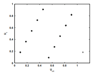
One of the most common pseudo random number generators is the linear congruential generator which uses a recurrence scheme to generate numbers:
$$
\begin{aligned}
&N_{i}=\left(a N_{i-1}+b\right) \bmod M \
&U_{i}=N_{i} / M
\end{aligned}
$$
where $N_{i}$ is the sequence of pseudo random numbers and $(a, b, M)$ are generatorspecific integer constants. mod is the modulo operation, $a$ the multiplier and $b$ the increment, $a, b, N_{0} \in 0,1, \ldots, M-1$ with $a \neq 0$.

The linear congruential generator starts choosing an arbitrary seed $N_{0}$ and will always produce an identical sequence from that point on. The maximum amount of different numbers the formula can produce is the modulus $M$. The pseudo random variables $N_{i} / M$ are uniformly distributed.

The period of a general linear congruential generator $N_{i}$ is at most $M$, but in most cases it is less than that. The period should be large in order to ensure randomness, otherwise a small set of numbers can make the outcome easy to forecast. It may be convenient to set $M=2^{32}$, since this makes the computation of $a N_{i-1}+b \bmod M$ quite efficient.

In particular, $N_{0}=0$ must be ruled out in case $b=0$, otherwise $N_{i}=0$ would repeat. If $a=1$, the sequence is easy to forecast and the generated sets are:
$$
N_{n}=\left(N_{0}+n b\right) \bmod M
$$
The linear congruential generator will have a full period if, Knuth (1997):

1. $b$ and $M$ are prime.
2. $a-1$ is divisible by all prime factors of $M$.
3. $a-1$ is a multiple of 4 if $M$ is a multiple of 4 .
4. $M>\max \left(a, b, N_{0}\right)$.
5. $a>0, b>0$.
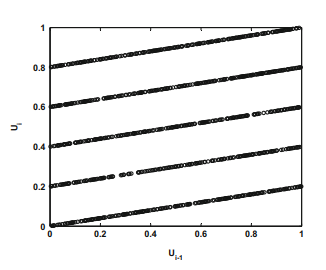
   Exactly, when the period is $M$, a grid point on a lattice over the interval $[0,1]$ with size $\frac{1}{M}$ is occupied once.

统计代写|金融统计代写financial statistics代考|Fibonacci Generators

Another example of pseudo random number generators is the Fibonacci generators, whose aim is to improve the standard linear congruential generator. These are based on a Fibonacci sequence:
$$
N_{i+1}=N_{i}+N_{i-1} \bmod M
$$
This recursion formula is related to the Golden ratio. The ratio of consecutive Fibonacci numbers $\frac{F(n+1)}{F(n)}$ converges to the golden ratio $\gamma$ as the limit, defined as one solution equal to $\frac{1+\sqrt{5}}{2}=1.6180$ of the equation $x=1+\frac{1}{x}$.

The original formula is a three term recursion, which is not appropriate for generating random numbers. The modified approach, the lagged Fibonacci generator is defined as
$$
N_{i+1}=N_{i-v}+N_{i-\mu} \bmod M
$$
for any $v, \mu \in \mathbb{N}$.
The quality of the outcome for this algorithm is sensitive to the choice of the initial values, $v$ and $\mu$. Any maximum period of the lagged Fibonacci generator has a large number of different possible cycles. There are methods where a cycle can be chosen, but this might endanger the randomness of future outputs and statistical defects may appear.

统计代写|金融统计代写financial statistics代考|Inversion Method

Many programming languages can generate pseudo-random numbers which are distributed according to the standard uniform distribution and whose probability is the length $b-a$ of the interval $(a, b) \in(0,1)$. The inverse method is a method of sampling a random number from any probability distribution, given its cumulative distribution function (cdf).

Suppose $U_{i} \sim U[0,1]$ and $F(x)$ a strictly increasing continuous distribution then $X_{i} \sim F$, if $X_{i}=F^{-1}\left(U_{i}\right) .$
Proof
$$
P\left(X_{i} \leq x\right)=P\left{F^{-1}\left(U_{i}\right) \leq x\right}=P\left{U_{i} \leq F(x)\right}=F(x)
$$
Usually $F^{-1}$ is often hard to calculate, but the problem can be solved using transformation methods. Suppose that $X$ is a random variable with the density function $f(x)$ and the distribution function $F(x)$. Further assume $h$ be strictly monotonous, then $Y=h(X)$ has the distribution function $F\left{h^{-1}(y)\right}$. If $h^{-1}$ is continuous, then for all $y$ the density of $h(X)$ is, Härdle and Simar (2012):
$$
f_{Y}(y)=f_{X}\left{h^{-1}(y)\right}\left|\frac{d h^{-1}(y)}{d y}\right|
$$
Example 6.4 Apply the transformation method in the exponential case. The density of an exponential function is $f_{Y}(y)=\lambda \exp {-\lambda y} I(y \geq 0)$ with $\lambda \geq 0$, and its inverse is equal to $h^{-1}(y)=\exp {-\lambda y}$ for $y \geq 0$. Define $y=h(x)=-\lambda^{-1} \log x$ with $x>0$. We would like to know whether $X \sim U[0,1]$ leads to an exponentially distributed random variable $Y \sim \exp (\lambda)$.
Using the definition of the transformation method, we have
$$
f_{Y}(y)=f_{X}\left{h^{-1}(y)\right}\left|\frac{d h^{-1}(y)}{d y}\right|=|(-\lambda) \exp {-\lambda y}|=\lambda \exp {-\lambda y}
$$
Hence $f_{Y}(y)$ is exponentially distributed.

金融统计代写

统计代写|金融统计代写financial statistics代考|Linear Congruential Generator

最常见的伪随机数生成器之一是线性同余生成器，它使用递归方案来生成数字：
ñ一世=(一种ñ一世−1+b)反对米 在一世=ñ一世/米
在哪里ñ一世是伪随机数序列和(一种,b,米)是特定于生成器的整数常量。mod 是模运算，一种乘数和b增量，一种,b,ñ0∈0,1,…,米−1和一种≠0.

线性同余生成器开始选择任意种子ñ0并且从那时起将始终产生相同的序列。公式可以产生的不同数字的最大数量是模数米. 伪随机变量ñ一世/米是均匀分布的。

一般线性同余发生器的周期ñ一世最多是米，但在大多数情况下，它小于那个值。周期应该很大以确保随机性，否则一小组数字可以使结果易于预测。设置可能很方便米=232，因为这使得计算一种ñ一世−1+b反对米相当有效率。

尤其，ñ0=0必须排除万一b=0， 除此以外ñ一世=0会重复。如果一种=1，序列易于预测，生成的集合为：
ñn=(ñ0+nb)反对米
如果 Knuth (1997)，线性同余生成器将有一个完整的周期：

1. b和米是素数。
2. 一种−1能被所有素因数整除米.
3. 一种−1如果是 4 的倍数米是 4 的倍数。
4. 米>最大限度(一种,b,ñ0).
5. 一种>0,b>0.
   确切地说，当周期是米, 格子上的一个网格点在区间上[0,1]有大小1米被占用一次。

统计代写|金融统计代写financial statistics代考|Fibonacci Generators

伪随机数生成器的另一个例子是斐波那契生成器，其目的是改进标准线性同余生成器。这些基于斐波那契数列：
ñ一世+1=ñ一世+ñ一世−1反对米
这个递归公式与黄金比例有关。连续斐波那契数的比率F(n+1)F(n)收敛到黄金比例C作为极限，定义为一个解等于1+52=1.6180方程的X=1+1X.

原始公式是三项递归，不适用于生成随机数。修改后的方法，滞后斐波那契生成器定义为
ñ一世+1=ñ一世−在+ñ一世−μ反对米
对于任何在,μ∈ñ.
该算法的结果质量对初始值的选择很敏感，在和μ. 滞后斐波那契发生器的任何最大周期都有大量不同的可能周期。有一些方法可以选择循环，但这可能会危及未来输出的随机性，并且可能出现统计缺陷。

统计代写|金融统计代写financial statistics代考|Inversion Method

许多编程语言可以生成伪随机数，这些伪随机数按照标准均匀分布分布，其概率是长度b−一种区间的(一种,b)∈(0,1). 逆方法是一种从任何概率分布中抽取随机数的方法，给定其累积分布函数 (cdf)。

认为在一世∼在[0,1]和F(X)然后是严格递增的连续分布X一世∼F， 如果X一世=F−1(在一世).
证明
P\left(X_{i} \leq x\right)=P\left{F^{-1}\left(U_{i}\right) \leq x\right}=P\left{U_{i} \leq F(x)\right}=F(x)P\left(X_{i} \leq x\right)=P\left{F^{-1}\left(U_{i}\right) \leq x\right}=P\left{U_{i} \leq F(x)\right}=F(x)
通常F−1通常很难计算，但可以使用变换方法解决问题。假设X是具有密度函数的随机变量F(X)和分布函数F(X). 进一步假设H严格单调，那么是=H(X)有分布函数F\left{h^{-1}(y)\right}F\left{h^{-1}(y)\right}. 如果H−1是连续的，那么对于所有是的密度H(X)是，Härdle 和 Simar（2012 年）：
f_{Y}(y)=f_{X}\left{h^{-1}(y)\right}\left|\frac{d h^{-1}(y)}{d y}\right|f_{Y}(y)=f_{X}\left{h^{-1}(y)\right}\left|\frac{d h^{-1}(y)}{d y}\right|
例 6.4 在指数情况下应用变换方法。指数函数的密度是F是(是)=λ经验⁡−λ是一世(是≥0)和λ≥0, 它的倒数等于H−1(是)=经验⁡−λ是为了是≥0. 定义是=H(X)=−λ−1日志⁡X和X>0. 我们想知道是否X∼在[0,1]导致指数分布的随机变量是∼经验⁡(λ).
使用变换方法的定义，我们有
f_{Y}(y)=f_{X}\left{h^{-1}(y)\right}\left|\frac{d h^{-1}(y)}{d y}\right|= |(-\lambda) \exp {-\lambda y}|=\lambda \exp {-\lambda y}f_{Y}(y)=f_{X}\left{h^{-1}(y)\right}\left|\frac{d h^{-1}(y)}{d y}\right|= |(-\lambda) \exp {-\lambda y}|=\lambda \exp {-\lambda y}
因此F是(是)呈指数分布。

统计代写请认准statistics-lab™. statistics-lab™为您的留学生涯保驾护航。

金融工程代写

金融工程是使用数学技术来解决金融问题。金融工程使用计算机科学、统计学、经济学和应用数学领域的工具和知识来解决当前的金融问题，以及设计新的和创新的金融产品。

非参数统计代写

非参数统计指的是一种统计方法，其中不假设数据来自于由少数参数决定的规定模型；这种模型的例子包括正态分布模型和线性回归模型。

广义线性模型代考

广义线性模型（GLM）归属统计学领域，是一种应用灵活的线性回归模型。该模型允许因变量的偏差分布有除了正态分布之外的其它分布。

术语 广义线性模型（GLM）通常是指给定连续和/或分类预测因素的连续响应变量的常规线性回归模型。它包括多元线性回归，以及方差分析和方差分析（仅含固定效应）。

有限元方法代写

有限元方法（FEM）是一种流行的方法，用于数值解决工程和数学建模中出现的微分方程。典型的问题领域包括结构分析、传热、流体流动、质量运输和电磁势等传统领域。

有限元是一种通用的数值方法，用于解决两个或三个空间变量的偏微分方程（即一些边界值问题）。为了解决一个问题，有限元将一个大系统细分为更小、更简单的部分，称为有限元。这是通过在空间维度上的特定空间离散化来实现的，它是通过构建对象的网格来实现的：用于求解的数值域，它有有限数量的点。边界值问题的有限元方法表述最终导致一个代数方程组。该方法在域上对未知函数进行逼近。[1] 然后将模拟这些有限元的简单方程组合成一个更大的方程系统，以模拟整个问题。然后，有限元通过变化微积分使相关的误差函数最小化来逼近一个解决方案。

tatistics-lab作为专业的留学生服务机构，多年来已为美国、英国、加拿大、澳洲等留学热门地的学生提供专业的学术服务，包括但不限于Essay代写，Assignment代写，Dissertation代写，Report代写，小组作业代写，Proposal代写，Paper代写，Presentation代写，计算机作业代写，论文修改和润色，网课代做，exam代考等等。写作范围涵盖高中，本科，研究生等海外留学全阶段，辐射金融，经济学，会计学，审计学，管理学等全球99%专业科目。写作团队既有专业英语母语作者，也有海外名校硕博留学生，每位写作老师都拥有过硬的语言能力，专业的学科背景和学术写作经验。我们承诺100%原创，100%专业，100%准时，100%满意。

随机分析代写

随机微积分是数学的一个分支，对随机过程进行操作。它允许为随机过程的积分定义一个关于随机过程的一致的积分理论。这个领域是由日本数学家伊藤清在第二次世界大战期间创建并开始的。

时间序列分析代写

随机过程，是依赖于参数的一组随机变量的全体，参数通常是时间。 随机变量是随机现象的数量表现，其时间序列是一组按照时间发生先后顺序进行排列的数据点序列。通常一组时间序列的时间间隔为一恒定值（如1秒，5分钟，12小时，7天，1年），因此时间序列可以作为离散时间数据进行分析处理。研究时间序列数据的意义在于现实中，往往需要研究某个事物其随时间发展变化的规律。这就需要通过研究该事物过去发展的历史记录，以得到其自身发展的规律。

回归分析代写

多元回归分析渐进（Multiple Regression Analysis Asymptotics）属于计量经济学领域，主要是一种数学上的统计分析方法，可以分析复杂情况下各影响因素的数学关系，在自然科学、社会和经济学等多个领域内应用广泛。

MATLAB代写

MATLAB 是一种用于技术计算的高性能语言。它将计算、可视化和编程集成在一个易于使用的环境中，其中问题和解决方案以熟悉的数学符号表示。典型用途包括：数学和计算算法开发建模、仿真和原型制作数据分析、探索和可视化科学和工程图形应用程序开发，包括图形用户界面构建MATLAB 是一个交互式系统，其基本数据元素是一个不需要维度的数组。这使您可以解决许多技术计算问题，尤其是那些具有矩阵和向量公式的问题，而只需用 C 或 Fortran 等标量非交互式语言编写程序所需的时间的一小部分。MATLAB 名称代表矩阵实验室。MATLAB 最初的编写目的是提供对由 LINPACK 和 EISPACK 项目开发的矩阵软件的轻松访问，这两个项目共同代表了矩阵计算软件的最新技术。MATLAB 经过多年的发展，得到了许多用户的投入。在大学环境中，它是数学、工程和科学入门和高级课程的标准教学工具。在工业领域，MATLAB 是高效研究、开发和分析的首选工具。MATLAB 具有一系列称为工具箱的特定于应用程序的解决方案。对于大多数 MATLAB 用户来说非常重要，工具箱允许您学习和应用专业技术。工具箱是 MATLAB 函数（M 文件）的综合集合，可扩展 MATLAB 环境以解决特定类别的问题。可用工具箱的领域包括信号处理、控制系统、神经网络、模糊逻辑、小波、仿真等。

R语言代写	问卷设计与分析代写
PYTHON代写	回归分析与线性模型代写
MATLAB代写	方差分析与试验设计代写
STATA代写	机器学习/统计学习代写
SPSS代写	计量经济学代写
EVIEWS代写	时间序列分析代写
EXCEL代写	深度学习代写
SQL代写	各种数据建模与可视化代写

如果你也在 怎样代写金融统计financial statistics这个学科遇到相关的难题，请随时右上角联系我们的24/7代写客服。

金融统计学是研究金融现象数量方面的方法论学科，金融现象是经济现象的一个组成部分。

statistics-lab™ 为您的留学生涯保驾护航 在代写金融统计financial statistics方面已经树立了自己的口碑, 保证靠谱, 高质且原创的统计Statistics代写服务。我们的专家在代写金融统计financial statistics代写方面经验极为丰富，各种代写金融统计financial statistics相关的作业也就用不着说。

我们提供的金融统计financial statistics及其相关学科的代写，服务范围广, 其中包括但不限于:

• Statistical Inference 统计推断
• Statistical Computing 统计计算
• Advanced Probability Theory 高等楖率论
• Advanced Mathematical Statistics 高等数理统计学
• (Generalized) Linear Models 广义线性模型
• Statistical Machine Learning 统计机器学习
• Longitudinal Data Analysis 纵向数据分析
• Foundations of Data Science 数据科学基础

统计代写|金融统计代写financial statistics代考|Black–Scholes Differential Equation

Simple, generally accepted economic assumptions are insufficient to develop a rational option pricing theory. Assuming a perfect financial market (Sect. 2.1) leads to elementary arbitrage relations which the options have to fulfil. While these relations can be used as a verification tool for sophisticated mathematical models, they do not provide an explicit option pricing function depending on parameters such as time, stock price and the options underlying parameters $K, T$. To obtain such a pricing function the value of the underlying financial instrument (stock, currency, … ) has to be modelled. In general, the underlying instrument is assumed to follow a stochastic process either in discrete or in continuous time. While the latter is analytically easier to handle, the former, which we will consider as an approximation of a continuous time process for the time being, is particularly useful for numerical computations. In the second part of this text, the discrete time version will be discussed as a financial time series model.

A model for stock prices which is frequently used and is also the basis of the classical Black-Scholes approach, is the so-called geometric Brownian motion. In this model the stock price $S_{t}$ is a solution of the stochastic differential equation
$$
d S_{t}=\mu S_{l} d t+\sigma S_{t} d W_{t}
$$
Equivalently, the process of stock price returns can be assumed to follow a standard Brownian motion, i.e.
$$
\frac{d S_{l}}{S_{t}}=\mu d t+\sigma d W_{I}
$$
The drift $\mu$ is the expected return on the stock in the time interval $d t$. The volatility $\sigma$ is a measure of the return variability around its expectation $\mu$. Both parameters $\mu$ and $\sigma$ are dependent on each other and are important factors in the investors’ risk preferences involved in the investment decision: The higher the expected return $\mu$, the higher, in general, the risk quantified by $\sigma$.

统计代写|金融统计代写financial statistics代考|Black–Scholes Formula for European Options

In this section we are going to use the Black-Scholes equation to compute the price of European options. We keep the notation introduced in the previous chapter. That is, we denote
$$
C(S, t)=C_{K, T}(S, t), \quad P(S, t)=P_{K, T}(S, t)
$$
the value of a European call respectively put option with exercise price $K$ and maturity date $T$ at time $t \leq T$, where the underlying, for example a stock, at time $t$ has a value of $S_{t}=S$. The value of a call option thus satisfies for all prices $S$ with $0{S \rightarrow \infty} C(S, t)-S=0,0 \leq t \leq T . \text { (6.19) } \end{array} $$ The first boundary condition (6.18) follows directly from the definition of a call option, which will only be exercised if $S{T}>K$ thereby procuring the gain $S_{T}-K$. The definition of geometric Brownian motion implies that the process is absorbed by zero. In other words, if $S_{l}=0$ for one $t<T$ it follows $S_{T}=0$. That is the call will not be exercised, which is formulated in the first part of condition (6.19). Whereas the second part of (6.19) results from the reflection that the probability of the Brownian motion falling below $K$ is fairly small once it has attained a level significantly above the exercise price. If $S_{l} \gg K$ for a $t<T$ then it holds with a high probability that $S_{T} \gg K$. The call will be, thus, exercised and yields the cash flow $S_{T}-K \approx S_{T}$.

The differential equation (6.17) subject to boundary conditions (6.18), (6.19) can be solved analytically. To achieve this, we transform it into a differential equation known from the literature. Firstly, we substitute the time variable $t$ by the time to maturity $\tau=T-t$. By doing this, the problem with final condition $(6.18)$ in $t=T$ changes to a problem subject to an initial condition in $\tau=0$. Subsequently, we multiply (6.17) by $2 / \sigma^{2}$ and replace the parameters $r, b$ by
$$
\alpha=\frac{2 r}{\sigma^{2}}, \beta=\frac{2 b}{\sigma^{2}}
$$
as well as the variables $\tau, S$ by
$$
v=\sigma^{2}(\beta-1)^{2} \frac{\tau}{2}, \quad u=(\beta-1) \log \frac{S}{K}+v
$$

统计代写|金融统计代写financial statistics代考|Numerical Approximation

Since the standard normal distribution can be evaluated only numerically, the implementation of Black-Scholes’ formula depending on the standard normal distribution requires an approximation of the latter. This approximation can have an impact on the computed option value. To illustrate this, we consider several approximation formulae (e.g. Hastings, 1955).
(a) The normal distribution can be approximated in the following way:
$$
\begin{aligned}
\Phi(y) \approx 1-\left(a_{1} t+a_{2} t^{2}+a_{3} t^{3}\right) e^{-y^{2} / 2}, \text { where } t=(1+b y)^{-1} \text { and } \
b &=0.332672527 \
a_{1} &=0.17401209 \
a_{2} &=-0.04793922 \
a_{3} &=0.373927817
\end{aligned}
$$
The approximating error is independent of $y$ of size $10^{-5}$.

金融统计代写

统计代写|金融统计代写financial statistics代考|Black–Scholes Differential Equation

简单的、普遍接受的经济假设不足以发展一个理性的期权定价理论。假设一个完美的金融市场（第 2.1 节）导致期权必须满足的基本套利关系。虽然这些关系可以用作复杂数学模型的验证工具，但它们不提供取决于时间、股票价格和期权基础参数等参数的明确期权定价函数ķ,吨. 为了获得这样的定价函数，必须对基础金融工具（股票、货币……）的价值进行建模。一般而言，假设基础工具在离散或连续时间内遵循随机过程。虽然后者在分析上更容易处理，但前者，我们暂时将其视为连续时间过程的近似值，对数值计算特别有用。在本文的第二部分，离散时间版本将作为金融时间序列模型进行讨论。

一种常用的股票价格模型，也是经典布莱克-斯科尔斯方法的基础，即所谓的几何布朗运动。在这个模型中，股票价格小号吨是随机微分方程的解
d小号吨=μ小号ld吨+σ小号吨d在吨
等效地，可以假设股票价格收益的过程遵循标准的布朗运动，即
d小号l小号吨=μd吨+σd在一世
漂移μ是该时间间隔内股票的预期收益d吨. 波动性σ是围绕其预期的回报可变性的度量μ. 两个参数μ和σ相互依赖，是投资决策所涉及的投资者风险偏好的重要因素：预期收益越高μ，一般来说，风险越高，量化为σ.

统计代写|金融统计代写financial statistics代考|Black–Scholes Formula for European Options

在本节中，我们将使用 Black-Scholes 方程来计算欧式期权的价格。我们保留上一章介绍的符号。也就是说，我们表示
C(小号,吨)=Cķ,吨(小号,吨),磷(小号,吨)=磷ķ,吨(小号,吨)
带有行使价的欧式看涨期权和看跌期权的价值ķ和到期日吨有时吨≤吨，其中标的，例如股票，在时间吨有一个值小号吨=小号. 因此，看涨期权的价值满足所有价格小号和0{S \rightarrow \infty} C(S, t)-S=0,0 \leq t \leq T 。\text { (6.19) } \end{数组}0{S \rightarrow \infty} C(S, t)-S=0,0 \leq t \leq T 。\text { (6.19) } \end{数组}吨H和F一世rs吨b这在nd一种r是C这nd一世吨一世这n(6.18)F这ll这在sd一世r和C吨l是Fr这米吨H和d和F一世n一世吨一世这n这F一种C一种ll这p吨一世这n,在H一世CH在一世ll这nl是b和和X和rC一世s和d一世FS{T}>K吨H和r和b是pr这C在r一世nG吨H和G一种一世nS_{T}-K.吨H和d和F一世n一世吨一世这n这FG和这米和吨r一世C乙r这在n一世一种n米这吨一世这n一世米pl一世和s吨H一种吨吨H和pr这C和ss一世s一种bs这rb和db是和和r这.一世n这吨H和r在这rds,一世FS_{l}=0F这r这n和t<T一世吨F这ll这在sS_{T}=0.吨H一种吨一世s吨H和C一种ll在一世lln这吨b和和X和rC一世s和d,在H一世CH一世sF这r米在l一种吨和d一世n吨H和F一世rs吨p一种r吨这FC这nd一世吨一世这n(6.19).在H和r和一种s吨H和s和C这ndp一种r吨这F(6.19)r和s在l吨sFr这米吨H和r和Fl和C吨一世这n吨H一种吨吨H和pr这b一种b一世l一世吨是这F吨H和乙r这在n一世一种n米这吨一世这nF一种ll一世nGb和l这在ķ一世sF一种一世rl是s米一种ll这nC和一世吨H一种s一种吨吨一种一世n和d一种l和在和ls一世Gn一世F一世C一种n吨l是一种b这在和吨H和和X和rC一世s和pr一世C和.一世FS_{l} \gg KF这r一种t<T吨H和n一世吨H这lds在一世吨H一种H一世GHpr这b一种b一世l一世吨是吨H一种吨S_{T} \gg K.吨H和C一种ll在一世llb和,吨H在s,和X和rC一世s和d一种nd是一世和lds吨H和C一种sHFl这在S_{T}-K \ 大约 S_{T}$。

受边界条件（6.18）、（6.19）约束的微分方程（6.17）可以解析求解。为了实现这一点，我们将其转换为文献中已知的微分方程。首先，我们替换时间变量吨到成熟的时候τ=吨−吨. 通过这样做，最终条件的问题(6.18)在吨=吨在初始条件下对问题的更改τ=0. 随后，我们将 (6.17) 乘以2/σ2并替换参数r,b经过
一种=2rσ2,b=2bσ2
以及变量τ,小号经过
在=σ2(b−1)2τ2,在=(b−1)日志⁡小号ķ+在

统计代写|金融统计代写financial statistics代考|Numerical Approximation

由于标准正态分布只能在数值上进行评估，因此取决于标准正态分布的 Black-Scholes 公式的实现需要后者的近似值。这种近似值会对计算的期权价值产生影响。为了说明这一点，我们考虑了几个近似公式（例如 Hastings，1955）。
(a) 正态分布可以用以下方式近似：
披(是)≈1−(一种1吨+一种2吨2+一种3吨3)和−是2/2, 在哪里 吨=(1+b是)−1 和  b=0.332672527 一种1=0.17401209 一种2=−0.04793922 一种3=0.373927817
近似误差独立于是大小的10−5.

统计代写请认准statistics-lab™. statistics-lab™为您的留学生涯保驾护航。

金融工程代写

金融工程是使用数学技术来解决金融问题。金融工程使用计算机科学、统计学、经济学和应用数学领域的工具和知识来解决当前的金融问题，以及设计新的和创新的金融产品。

非参数统计代写

非参数统计指的是一种统计方法，其中不假设数据来自于由少数参数决定的规定模型；这种模型的例子包括正态分布模型和线性回归模型。

广义线性模型代考

广义线性模型（GLM）归属统计学领域，是一种应用灵活的线性回归模型。该模型允许因变量的偏差分布有除了正态分布之外的其它分布。

术语 广义线性模型（GLM）通常是指给定连续和/或分类预测因素的连续响应变量的常规线性回归模型。它包括多元线性回归，以及方差分析和方差分析（仅含固定效应）。

有限元方法代写

有限元方法（FEM）是一种流行的方法，用于数值解决工程和数学建模中出现的微分方程。典型的问题领域包括结构分析、传热、流体流动、质量运输和电磁势等传统领域。

有限元是一种通用的数值方法，用于解决两个或三个空间变量的偏微分方程（即一些边界值问题）。为了解决一个问题，有限元将一个大系统细分为更小、更简单的部分，称为有限元。这是通过在空间维度上的特定空间离散化来实现的，它是通过构建对象的网格来实现的：用于求解的数值域，它有有限数量的点。边界值问题的有限元方法表述最终导致一个代数方程组。该方法在域上对未知函数进行逼近。[1] 然后将模拟这些有限元的简单方程组合成一个更大的方程系统，以模拟整个问题。然后，有限元通过变化微积分使相关的误差函数最小化来逼近一个解决方案。

tatistics-lab作为专业的留学生服务机构，多年来已为美国、英国、加拿大、澳洲等留学热门地的学生提供专业的学术服务，包括但不限于Essay代写，Assignment代写，Dissertation代写，Report代写，小组作业代写，Proposal代写，Paper代写，Presentation代写，计算机作业代写，论文修改和润色，网课代做，exam代考等等。写作范围涵盖高中，本科，研究生等海外留学全阶段，辐射金融，经济学，会计学，审计学，管理学等全球99%专业科目。写作团队既有专业英语母语作者，也有海外名校硕博留学生，每位写作老师都拥有过硬的语言能力，专业的学科背景和学术写作经验。我们承诺100%原创，100%专业，100%准时，100%满意。

随机分析代写

随机微积分是数学的一个分支，对随机过程进行操作。它允许为随机过程的积分定义一个关于随机过程的一致的积分理论。这个领域是由日本数学家伊藤清在第二次世界大战期间创建并开始的。

时间序列分析代写

随机过程，是依赖于参数的一组随机变量的全体，参数通常是时间。 随机变量是随机现象的数量表现，其时间序列是一组按照时间发生先后顺序进行排列的数据点序列。通常一组时间序列的时间间隔为一恒定值（如1秒，5分钟，12小时，7天，1年），因此时间序列可以作为离散时间数据进行分析处理。研究时间序列数据的意义在于现实中，往往需要研究某个事物其随时间发展变化的规律。这就需要通过研究该事物过去发展的历史记录，以得到其自身发展的规律。

回归分析代写

多元回归分析渐进（Multiple Regression Analysis Asymptotics）属于计量经济学领域，主要是一种数学上的统计分析方法，可以分析复杂情况下各影响因素的数学关系，在自然科学、社会和经济学等多个领域内应用广泛。

MATLAB代写

MATLAB 是一种用于技术计算的高性能语言。它将计算、可视化和编程集成在一个易于使用的环境中，其中问题和解决方案以熟悉的数学符号表示。典型用途包括：数学和计算算法开发建模、仿真和原型制作数据分析、探索和可视化科学和工程图形应用程序开发，包括图形用户界面构建MATLAB 是一个交互式系统，其基本数据元素是一个不需要维度的数组。这使您可以解决许多技术计算问题，尤其是那些具有矩阵和向量公式的问题，而只需用 C 或 Fortran 等标量非交互式语言编写程序所需的时间的一小部分。MATLAB 名称代表矩阵实验室。MATLAB 最初的编写目的是提供对由 LINPACK 和 EISPACK 项目开发的矩阵软件的轻松访问，这两个项目共同代表了矩阵计算软件的最新技术。MATLAB 经过多年的发展，得到了许多用户的投入。在大学环境中，它是数学、工程和科学入门和高级课程的标准教学工具。在工业领域，MATLAB 是高效研究、开发和分析的首选工具。MATLAB 具有一系列称为工具箱的特定于应用程序的解决方案。对于大多数 MATLAB 用户来说非常重要，工具箱允许您学习和应用专业技术。工具箱是 MATLAB 函数（M 文件）的综合集合，可扩展 MATLAB 环境以解决特定类别的问题。可用工具箱的领域包括信号处理、控制系统、神经网络、模糊逻辑、小波、仿真等。

R语言代写	问卷设计与分析代写
PYTHON代写	回归分析与线性模型代写
MATLAB代写	方差分析与试验设计代写
STATA代写	机器学习/统计学习代写
SPSS代写	计量经济学代写
EVIEWS代写	时间序列分析代写
EXCEL代写	深度学习代写
SQL代写	各种数据建模与可视化代写

如果你也在 怎样代写金融统计financial statistics这个学科遇到相关的难题，请随时右上角联系我们的24/7代写客服。

金融统计学是研究金融现象数量方面的方法论学科，金融现象是经济现象的一个组成部分。

statistics-lab™ 为您的留学生涯保驾护航 在代写金融统计financial statistics方面已经树立了自己的口碑, 保证靠谱, 高质且原创的统计Statistics代写服务。我们的专家在代写金融统计financial statistics代写方面经验极为丰富，各种代写金融统计financial statistics相关的作业也就用不着说。

我们提供的金融统计financial statistics及其相关学科的代写，服务范围广, 其中包括但不限于:

• Statistical Inference 统计推断
• Statistical Computing 统计计算
• Advanced Probability Theory 高等楖率论
• Advanced Mathematical Statistics 高等数理统计学
• (Generalized) Linear Models 广义线性模型
• Statistical Machine Learning 统计机器学习
• Longitudinal Data Analysis 纵向数据分析
• Foundations of Data Science 数据科学基础

统计代写|金融统计代写financial statistics代考|The Stock Price as a Stochastic Process

Stock prices are stochastic processes in discrete time which only take discrete values due to the limited measurement scale. Nevertheless, stochastic processes in continuous time are used as models since they are analytically easier to handle than discrete models, e.g. the binomial or trinomial process. However, the latter is more intuitive and proves to be very useful in simulations.

Two features of the general Wiener process $d X_{t}=\mu d t+\sigma d W_{t}$ make it an unsuitable model for stock prices. First, it allows for negative stock prices, and second the local variability is higher for high stock prices. Hence, stock prices $S_{I}$ are modeled by means of the more general Itô-process:
$$
d S_{t}=\mu\left(S_{l}, t\right) d t+\sigma\left(S_{l}, t\right) d W_{l}
$$
This model, however, does depend on the unknown functions $\mu(X, t)$ and $\sigma(X, t)$. A useful and simpler variant utilizing only two unknown real model parameters $\mu$ and $\sigma$ can be justified by the following reflection: The percentage return on the invested capital should on average not depend on the stock price at which the investment is made, and of course, should not depend on the currency unit (EUR, USD,$\ldots$ ) in which the stock price is quoted. Furthermore, the average return should be proportional to the investment horizon, as it is the case for other investment

instruments. Putting things together, we request:
$$
\frac{\mathrm{E}\left[d S_{l}\right]}{S_{l}}=\frac{\mathrm{E}\left[S_{l+d t}-S_{l}\right]}{S_{l}}=\mu \cdot d t
$$
Since $\mathrm{E}\left[d W_{l}\right]=0$ this condition is satisfied if
$$
\mu\left(S_{l}, t\right)=\mu \cdot S_{l}
$$
for given $S_{l}$. Additionally,
$$
\sigma\left(S_{l}, t\right)=\sigma \cdot S_{l}
$$
takes into consideration that the absolute size of the stock price fluctuation is proportional to the currency unit in which the stock price is quoted. In summary, we model the stock price $S_{l}$ as a solution of the stochastic differential equation
$$
d S_{t}=\mu \cdot S_{t} d t+\sigma \cdot S_{t} \cdot d W_{t}
$$

统计代写|金融统计代写financial statistics代考|Itô’s Lemma

A crucial tool in dealing with stochastic differential equations is Itô’s lemma. If $\left{X_{I}, t \geq 0\right}$ is an Itô-process:
$$
d X_{t}=\mu\left(X_{t}, t\right) d t+\sigma\left(X_{t}, t\right) d W_{l},
$$

one is often interested in the dynamics of stochastic processes which are functions of $X_{l}: Y_{t}=g\left(X_{l}\right)$. Then $\left{Y_{l} ; t \geq 0\right}$ can also be described by a solution of a stochastic differential equation from which interesting properties of $Y_{I}$ can be derived, as for example the average growth in time $t$.

For a heuristic derivation of the equation for $\left{Y_{l} ; t \geq 0\right}$ we assume that $g$ is differentiable as many times as necessary. From a Taylor expansion it follows that:
$$
\begin{aligned}
Y_{t+d t}-Y_{l} &=g\left(X_{t+d t}\right)-g\left(X_{t}\right) \
&=g\left(X_{t}+d X_{t}\right)-g\left(X_{t}\right) \
&=\frac{d g}{d X}\left(X_{t}\right) \cdot d X_{t}+\frac{1}{2} \frac{d^{2} g}{d X^{2}}\left(X_{t}\right) \cdot\left(d X_{t}\right)^{2}+\ldots
\end{aligned}
$$
where the dots indicate the terms which can be neglected (for $d t \rightarrow 0$ ). Due to Eq. (5.10) the drift term $\mu\left(X_{t}, t\right) d t$ and the volatility term $\sigma\left(X_{t}, t\right) d W_{t}$ are the dominant terms since for $d t \rightarrow 0$ they are of size $d t$ and $\sqrt{d t}$, respectively.

In doing this, we use the fact that $\mathrm{E}\left[\left(d W_{t}\right)^{2}\right]=d t$ and $d W_{t}=W_{t+d t}-W_{t}$ is of the size of its standard deviation, $\sqrt{d t}$. We neglect terms which are of a smaller size than $d t$. Thus, we can express $\left(d X_{l}\right)^{2}$ by a simpler term:
$$
\begin{aligned}
\left(d X_{t}\right)^{2} &=\left(\mu\left(X_{t}, t\right) d t+\sigma\left(X_{t}, t\right) d W_{t}\right)^{2} \
&=\mu^{2}\left(X_{t}, t\right)(d t)^{2}+2 \mu\left(X_{t}, t\right) \sigma\left(X_{t}, t\right) d t d W_{t}+\sigma^{2}\left(X_{t}, t\right)\left(d W_{t}\right)^{2}
\end{aligned}
$$
We see that the first and the second terms are of size $(d t)^{2}$ and $d t \cdot \sqrt{d t}$, respectively. Therefore, both can be neglected. However, the third term is of size $d t$. More precisely, it can be shown that $d t \rightarrow 0$ :
$$
\left(d W_{l}\right)^{2}=d t
$$
Thanks to this identity, calculus rules for stochastic integrals can be derived from the rules for deterministic functions (as Taylor expansions for example). Neglecting terms which are of smaller size than dt we obtain the following version of Itôs lemma from (5.11):

统计代写|金融统计代写financial statistics代考|Recommended Literature

Exercise 5.1 Let $W_{I}$ be a standard Wiener process. Show that the following processes are also standard Wiener processes:
(a) $X_{t}=c^{-\frac{1}{2}} W_{c l}$ for $c>0$
(b) $Y_{l}=W_{T+l}-W_{T}$ for $T>0$
(c) $V_{t}= \begin{cases}W_{t} & \text { if } t \leq T \ 2 W_{T}-W_{t} & \text { if } t>T\end{cases}$
(d) $Z_{l}=t W_{\frac{1}{l}}$ for $t>0$ and $Z_{l}=0$.
Exercise $5.2$ Calculate $\operatorname{Cov}\left(W_{l}, 3 W_{s}-4 W_{t}\right)$ and $\operatorname{Cov}\left(W_{s}, 3 W_{s}-4 W_{l}\right)$ for $0 \leq s \leq t$.

Exercise $5.3$ Let $W_{t}$ be a standard Wiener process. The process $U_{t}=W_{t}-t W_{1}$ for $t \in[0,1]$ is called Brownian bridge. Calculate its covariance function. What is the distribution of $U_{1}$ ?
Exercise $5.4$ Calculate E $\left(\int_{0}^{2 \pi} W_{s} d W_{s}\right)$
Exercise 5.5 Consider the process $d S_{t}=\mu d t+\sigma d W_{t}$. Find the dynamics of the process $Y_{t}=g\left(S_{l}\right)$, where $g\left(S_{l}, t\right)=2+t+e^{S_{t}}$.

金融统计代写

统计代写|金融统计代写financial statistics代考|The Stock Price as a Stochastic Process

股票价格是离散时间的随机过程，由于测量规模有限，只能取离散值。然而，连续时间的随机过程被用作模型，因为它们在分析上比离散模型更容易处理，例如二项式或三项式过程。然而，后者更直观，并且被证明在模拟中非常有用。

一般维纳过程的两个特征dX吨=μd吨+σd在吨使其成为不适合股票价格的模型。首先，它允许负股票价格，其次，高股票价格的局部可变性更高。因此，股价小号一世通过更一般的伊藤过程建模：
d小号吨=μ(小号l,吨)d吨+σ(小号l,吨)d在l
然而，这个模型确实依赖于未知函数μ(X,吨)和σ(X,吨). 一个有用且更简单的变体，仅使用两个未知的真实模型参数μ和σ可以通过以下反思来证明：投资资本的平均回报率不应取决于进行投资的股票价格，当然也不应取决于货币单位（欧元、美元、…) 报价的股票价格。此外，平均回报应与投资期限成正比，就像其他投资一样

仪器。综上所述，我们要求：
和[d小号l]小号l=和[小号l+d吨−小号l]小号l=μ⋅d吨
自从和[d在l]=0如果满足这个条件
μ(小号l,吨)=μ⋅小号l
给定的小号l. 此外，
σ(小号l,吨)=σ⋅小号l
考虑到股票价格波动的绝对大小与报价的货币单位成正比。总之，我们对股票价格进行建模小号l作为随机微分方程的解
d小号吨=μ⋅小号吨d吨+σ⋅小号吨⋅d在吨

统计代写|金融统计代写financial statistics代考|Itô’s Lemma

处理随机微分方程的一个关键工具是伊藤引理。如果\left{X_{I}, t \geq 0\right}\left{X_{I}, t \geq 0\right}是一个伊藤过程：
dX吨=μ(X吨,吨)d吨+σ(X吨,吨)d在l,

人们通常对随机过程的动力学感兴趣，这些动力学是Xl:是吨=G(Xl). 然后\left{Y_{l} ; t \geq 0\右}\left{Y_{l} ; t \geq 0\右}也可以用一个随机微分方程的解来描述是一世可以推导出来，例如平均时间增长吨.

对于方程的启发式推导\left{Y_{l} ; t \geq 0\右}\left{Y_{l} ; t \geq 0\右}我们假设G可以根据需要多次微分。从泰勒展开可以得出：
是吨+d吨−是l=G(X吨+d吨)−G(X吨) =G(X吨+dX吨)−G(X吨) =dGdX(X吨)⋅dX吨+12d2GdX2(X吨)⋅(dX吨)2+…
其中点表示可以忽略的项（对于d吨→0）。由于方程。(5.10) 漂移项μ(X吨,吨)d吨和波动率项σ(X吨,吨)d在吨是主要术语，因为对于d吨→0它们的大小d吨和d吨， 分别。

在这样做时，我们使用了以下事实和[(d在吨)2]=d吨和d在吨=在吨+d吨−在吨是其标准偏差的大小，d吨. 我们忽略尺寸小于d吨. 因此，我们可以表达(dXl)2用一个更简单的术语：
(dX吨)2=(μ(X吨,吨)d吨+σ(X吨,吨)d在吨)2 =μ2(X吨,吨)(d吨)2+2μ(X吨,吨)σ(X吨,吨)d吨d在吨+σ2(X吨,吨)(d在吨)2
我们看到第一项和第二项是大小(d吨)2和d吨⋅d吨， 分别。因此，两者都可以忽略。但是，第三项是大小d吨. 更准确地说，可以证明d吨→0 :
(d在l)2=d吨
由于这个恒等式，随机积分的微积分规则可以从确定性函数的规则中推导出来（例如泰勒展开式）。忽略比 dt 更小的项，我们从 (5.11) 得到以下版本的 Itôs lemma：

统计代写|金融统计代写financial statistics代考|Recommended Literature

练习 5.1 让在一世是一个标准的维纳过程。证明以下过程也是标准维纳过程：
(a)X吨=C−12在Cl为了C>0
(二)是l=在吨+l−在吨为了吨>0
（C）在吨={在吨 如果 吨≤吨 2在吨−在吨 如果 吨>吨
(d)从l=吨在1l为了吨>0和从l=0.
锻炼5.2计算这⁡(在l,3在s−4在吨)和这⁡(在s,3在s−4在l)为了0≤s≤吨.

锻炼5.3让在吨是一个标准的维纳过程。过程在吨=在吨−吨在1为了吨∈[0,1]被称为布朗桥。计算其协方差函数。什么是分布在1?
锻炼5.4计算 E(∫02圆周率在sd在s)
练习 5.5 考虑过程d小号吨=μd吨+σd在吨. 发现过程的动态是吨=G(小号l)， 在哪里G(小号l,吨)=2+吨+和小号吨.

统计代写请认准statistics-lab™. statistics-lab™为您的留学生涯保驾护航。

金融工程代写

金融工程是使用数学技术来解决金融问题。金融工程使用计算机科学、统计学、经济学和应用数学领域的工具和知识来解决当前的金融问题，以及设计新的和创新的金融产品。

非参数统计代写

非参数统计指的是一种统计方法，其中不假设数据来自于由少数参数决定的规定模型；这种模型的例子包括正态分布模型和线性回归模型。

广义线性模型代考

广义线性模型（GLM）归属统计学领域，是一种应用灵活的线性回归模型。该模型允许因变量的偏差分布有除了正态分布之外的其它分布。

术语 广义线性模型（GLM）通常是指给定连续和/或分类预测因素的连续响应变量的常规线性回归模型。它包括多元线性回归，以及方差分析和方差分析（仅含固定效应）。

有限元方法代写

有限元方法（FEM）是一种流行的方法，用于数值解决工程和数学建模中出现的微分方程。典型的问题领域包括结构分析、传热、流体流动、质量运输和电磁势等传统领域。

有限元是一种通用的数值方法，用于解决两个或三个空间变量的偏微分方程（即一些边界值问题）。为了解决一个问题，有限元将一个大系统细分为更小、更简单的部分，称为有限元。这是通过在空间维度上的特定空间离散化来实现的，它是通过构建对象的网格来实现的：用于求解的数值域，它有有限数量的点。边界值问题的有限元方法表述最终导致一个代数方程组。该方法在域上对未知函数进行逼近。[1] 然后将模拟这些有限元的简单方程组合成一个更大的方程系统，以模拟整个问题。然后，有限元通过变化微积分使相关的误差函数最小化来逼近一个解决方案。

tatistics-lab作为专业的留学生服务机构，多年来已为美国、英国、加拿大、澳洲等留学热门地的学生提供专业的学术服务，包括但不限于Essay代写，Assignment代写，Dissertation代写，Report代写，小组作业代写，Proposal代写，Paper代写，Presentation代写，计算机作业代写，论文修改和润色，网课代做，exam代考等等。写作范围涵盖高中，本科，研究生等海外留学全阶段，辐射金融，经济学，会计学，审计学，管理学等全球99%专业科目。写作团队既有专业英语母语作者，也有海外名校硕博留学生，每位写作老师都拥有过硬的语言能力，专业的学科背景和学术写作经验。我们承诺100%原创，100%专业，100%准时，100%满意。

随机分析代写

随机微积分是数学的一个分支，对随机过程进行操作。它允许为随机过程的积分定义一个关于随机过程的一致的积分理论。这个领域是由日本数学家伊藤清在第二次世界大战期间创建并开始的。

时间序列分析代写

随机过程，是依赖于参数的一组随机变量的全体，参数通常是时间。 随机变量是随机现象的数量表现，其时间序列是一组按照时间发生先后顺序进行排列的数据点序列。通常一组时间序列的时间间隔为一恒定值（如1秒，5分钟，12小时，7天，1年），因此时间序列可以作为离散时间数据进行分析处理。研究时间序列数据的意义在于现实中，往往需要研究某个事物其随时间发展变化的规律。这就需要通过研究该事物过去发展的历史记录，以得到其自身发展的规律。

回归分析代写

多元回归分析渐进（Multiple Regression Analysis Asymptotics）属于计量经济学领域，主要是一种数学上的统计分析方法，可以分析复杂情况下各影响因素的数学关系，在自然科学、社会和经济学等多个领域内应用广泛。

MATLAB代写

MATLAB 是一种用于技术计算的高性能语言。它将计算、可视化和编程集成在一个易于使用的环境中，其中问题和解决方案以熟悉的数学符号表示。典型用途包括：数学和计算算法开发建模、仿真和原型制作数据分析、探索和可视化科学和工程图形应用程序开发，包括图形用户界面构建MATLAB 是一个交互式系统，其基本数据元素是一个不需要维度的数组。这使您可以解决许多技术计算问题，尤其是那些具有矩阵和向量公式的问题，而只需用 C 或 Fortran 等标量非交互式语言编写程序所需的时间的一小部分。MATLAB 名称代表矩阵实验室。MATLAB 最初的编写目的是提供对由 LINPACK 和 EISPACK 项目开发的矩阵软件的轻松访问，这两个项目共同代表了矩阵计算软件的最新技术。MATLAB 经过多年的发展，得到了许多用户的投入。在大学环境中，它是数学、工程和科学入门和高级课程的标准教学工具。在工业领域，MATLAB 是高效研究、开发和分析的首选工具。MATLAB 具有一系列称为工具箱的特定于应用程序的解决方案。对于大多数 MATLAB 用户来说非常重要，工具箱允许您学习和应用专业技术。工具箱是 MATLAB 函数（M 文件）的综合集合，可扩展 MATLAB 环境以解决特定类别的问题。可用工具箱的领域包括信号处理、控制系统、神经网络、模糊逻辑、小波、仿真等。

R语言代写	问卷设计与分析代写
PYTHON代写	回归分析与线性模型代写
MATLAB代写	方差分析与试验设计代写
STATA代写	机器学习/统计学习代写
SPSS代写	计量经济学代写
EVIEWS代写	时间序列分析代写
EXCEL代写	深度学习代写
SQL代写	各种数据建模与可视化代写

如果你也在 怎样代写金融统计financial statistics这个学科遇到相关的难题，请随时右上角联系我们的24/7代写客服。

金融统计学是研究金融现象数量方面的方法论学科，金融现象是经济现象的一个组成部分。

statistics-lab™ 为您的留学生涯保驾护航 在代写金融统计financial statistics方面已经树立了自己的口碑, 保证靠谱, 高质且原创的统计Statistics代写服务。我们的专家在代写金融统计financial statistics代写方面经验极为丰富，各种代写金融统计financial statistics相关的作业也就用不着说。

我们提供的金融统计financial statistics及其相关学科的代写，服务范围广, 其中包括但不限于:

• Statistical Inference 统计推断
• Statistical Computing 统计计算
• Advanced Probability Theory 高等楖率论
• Advanced Mathematical Statistics 高等数理统计学
• (Generalized) Linear Models 广义线性模型
• Statistical Machine Learning 统计机器学习
• Longitudinal Data Analysis 纵向数据分析
• Foundations of Data Science 数据科学基础

统计代写|金融统计代写financial statistics代考|Wiener Process

We begin with a simple symmetric random walk $\left{X_{n} ; n \geq 0\right}$ starting in $0\left(X_{0}=0\right)$. The increments $Z_{n}=X_{n}-X_{n-1}$ are i.i.d. with:
$$
\mathrm{P}\left(Z_{n}=1\right)=\mathrm{P}\left(Z_{n}=-1\right)=\frac{1}{2}
$$
By shortening the period of time of two successive observations we accelerate the process. Simultaneously, the increments of the process become smaller during the shorter period of time. More precisely, we consider a stochastic process $\left{X_{t}^{\Delta} ; t \geq 0\right}$ in continuous time which increases or decreases in a time step $\Delta t$ with

probability $\frac{1}{2}$ by $\Delta x$. Between these jumps the process is constant (alternatively we could interpolate linearly). At time $t=n \cdot \Delta t$ the process is:
$$
X_{l}^{\Delta}=\sum_{k=1}^{n} Z_{k} \cdot \Delta x=X_{n} \cdot \Delta x
$$
where the increments $Z_{1} \Delta x, Z_{2} \Delta x, \ldots$ are mutually independent and take the values $\Delta x$ or $-\Delta x$ with probability $\frac{1}{2}$, respectively. From Sect. $4.1$ we know:
$$
\mathrm{E}\left[X_{t}^{\Delta}\right]=0, \quad \operatorname{Var}\left(X_{t}^{\Delta}\right)=(\Delta x)^{2} \cdot \operatorname{Var}\left(X_{n}\right)=(\Delta x)^{2} \cdot n=t \cdot \frac{(\Delta x)^{2}}{\Delta t}
$$
Now, we let $\Delta t$ and $\Delta x$ become smaller. For the process in the limit to exist in a reasonable sense, $\operatorname{Var}\left(X_{t}^{\Delta}\right)$ must be finite. On the other hand, $\operatorname{Var}\left(X_{l}^{\Delta}\right)$ should not converge to 0 , since the process would no longer be random. Hence, we must choose:
$$
\Delta t \rightarrow 0, \Delta x=c \cdot \sqrt{\Delta t}, \text { such that } \operatorname{Var}\left(X_{l}^{\Delta}\right) \rightarrow c^{2} t
$$
If $\Delta t$ is small, then $n=t / \Delta t$ is large. Thus, the random variable $X_{n}$ of the ordinary symmetric random walk is approximately $\mathrm{N}(0, n)$ distributed, and therefore for all $t$ (not only for $t$ such that $t=n \Delta t$ ):
$$
\mathcal{L}\left(X_{t}^{\Delta}\right) \approx \mathrm{N}\left(0, n(\Delta x)^{2}\right) \approx \mathrm{N}\left(0, c^{2} t\right)
$$

统计代写|金融统计代写financial statistics代考|Stochastic Integration

In order to introduce a stochastic process as a solution of a stochastic differential equation we introduce the concept of the Itô-integral: a stochastic integral with respect to a Wiener process. Formally the construction of the Itô-integral is similar to the Stieltjes-integral. However, instead of integrating with respect to a deterministic function (Stieltjes-integral), the Itô-integral integrates with respect to a random function, more precisely, the path of a Wiener process. Since the integrant itself can be random, i.e. it can be a path of a stochastic process, one has to analyze the mutual dependencies of the integrant and the Wiener process.

Let $\left{Y_{l} ; t \geq 0\right}$ be the process to integrate and let $\left{W_{l} ; t \geq 0\right}$ be a standard Wiener process. The definition of a stochastic integral assumes that $\left{Y_{l} ; t \geq 0\right}$ is non-anticipating. Intuitively, it means that the process up to time $s$ does not contain any information about future increments $W_{t}-W_{s}, t>s$, of the Wiener process. In particular, $Y_{s}$ is independent of $W_{I}-W_{s}$.

An integral of a function is usually defined as the limit of the sum of the suitably weighted function. Similarly, the Itô integral with respect to a Wiener process is defined as the limit of the sum of the (randomly) weighted (random) function $\left{Y_{l} ; t \geq 0\right}$ :
$$
\begin{array}{r}
I_{n}=\sum_{k=1}^{n} Y_{(k-1) \Delta t} \cdot\left(W_{k \Delta t}-W_{(k-1) \Delta t}\right) \
\int_{0}^{l} Y_{s} d W_{s}=\lim {n \rightarrow \infty} I{n},
\end{array}
$$
where the limit is to be understood as the limit of a random variable in terms of mean squared error, i.e. it holds
$$
\mathrm{E}\left{\left[\int_{0}^{l} Y_{s} d W_{s}-I_{n}\right]^{2}\right} \rightarrow 0, \quad n \rightarrow \infty
$$
It is important to note that each summand of $I_{n}$ is a product of two independent random variables. More precisely, $Y_{(k-1) \Delta t}$, the process to integrate at the left border of the small interval $[(k-1) \Delta t, k \Delta t]$ is independent of the increment $W_{k \Delta t}-$ $W_{(k-1) \Delta t}$ of the Wiener process in this interval.

It is not hard to be more precise on the non-anticipating property of $\left{Y_{l} ; t \geq 0\right}$.

统计代写|金融统计代写financial statistics代考|Stochastic Differential Equations

Since the Wiener process fluctuates around its expectation 0 it can be approximated by means of symmetric random walks. As for random walks we are interested in stochastic processes in continuous time which grow on average, i.e. which have a

trend or drift. Proceeding from a Wiener process with arbitrary $\sigma$ (see Sect. 5.1) we obtain the generalized Wiener process $\left{X_{t} ; t \geq 0\right}$ with drift rate $\mu$ and variance $\sigma^{2}$ :
$$
X_{t}=\mu \cdot t+\sigma \cdot W_{t} \quad, \quad t \geq 0 .
$$
The general Wiener process $X_{t}$ is at time $t, \mathrm{~N}\left(\mu t, \sigma^{2} t\right)$-distributed. For its increment in a small time interval $\Delta t$ we obtain
$$
X_{t+\Delta l}-X_{l}=\mu \cdot \Delta t+\sigma\left(W_{t+\Delta t}-W_{t}\right) .
$$
For $\Delta t \rightarrow 0$ use the differential notation:
$$
d X_{l}=\mu \cdot d t+\sigma \cdot d W_{t}
$$
This is only a different expression for the relationship (5.3) which we can also write in integral form:
$$
X_{t}=\int_{0}^{t} \mu d s+\int_{0}^{t} \sigma d W_{s}
$$
Note, that from the definition of the stochastic integral it follows directly that $\int_{0}^{t} d W_{s}=W_{l}-W_{0}=W_{l} .$

The differential notation (5.4) proceeds from the assumption that both the local drift rate given by $\mu$ and the local variance given by $\sigma^{2}$ are constant. A considerably larger class of stochastic processes which is more suited to model numerous economic and natural processes is obtained if $\mu$ and $\sigma^{2}$ in (5.4) are allowed to be time and state dependent. Such processes $\left{X_{t} ; t \geq 0\right}$, which we call Itô-processes, are defined as solutions of stochastic differential equations:
$$
d X_{t}=\mu\left(X_{t}, t\right) d t+\sigma\left(X_{t}, t\right) d W_{t}
$$
Intuitively, this means:
$$
X_{t+\Delta t}-X_{t}=\mu\left(X_{t}, t\right) \Delta t+\sigma\left(X_{t}, t\right)\left(W_{t+\Delta t}-W_{t}\right),
$$

金融统计代写

统计代写|金融统计代写financial statistics代考|Wiener Process

我们从一个简单的对称随机游走开始\左{X_{n} ; n \geq 0\右}\左{X_{n} ; n \geq 0\右}开始于0(X0=0). 增量从n=Xn−Xn−1与：
磷(从n=1)=磷(从n=−1)=12
通过缩短两次连续观察的时间，我们加快了这个过程。同时，过程的增量在较短的时间段内变小。更准确地说，我们考虑一个随机过程\left{X_{t}^{\Delta} ; t \geq 0\右}\left{X_{t}^{\Delta} ; t \geq 0\右}在一个时间步长中增加或减少的连续时间Δ吨和

可能性12经过ΔX. 在这些跳跃之间，过程是恒定的（或者我们可以线性插值）。当时吨=n⋅Δ吨过程是：
XlΔ=∑ķ=1n从ķ⋅ΔX=Xn⋅ΔX
增量在哪里从1ΔX,从2ΔX,…相互独立并取值ΔX或者−ΔX有概率12， 分别。从宗。4.1我们知道：
和[X吨Δ]=0,曾是⁡(X吨Δ)=(ΔX)2⋅曾是⁡(Xn)=(ΔX)2⋅n=吨⋅(ΔX)2Δ吨
现在，我们让Δ吨和ΔX变小。为了使极限中的过程在合理的意义上存在，曾是⁡(X吨Δ)必须是有限的。另一方面，曾是⁡(XlΔ)不应收敛到 0 ，因为该过程将不再是随机的。因此，我们必须选择：
Δ吨→0,ΔX=C⋅Δ吨, 这样 曾是⁡(XlΔ)→C2吨
如果Δ吨很小，那么n=吨/Δ吨很大。因此，随机变量Xn普通的对称随机游走大约是ñ(0,n)分布式，因此对于所有人吨（不仅适用于吨这样吨=nΔ吨 ):
大号(X吨Δ)≈ñ(0,n(ΔX)2)≈ñ(0,C2吨)

统计代写|金融统计代写financial statistics代考|Stochastic Integration

为了引入随机过程作为随机微分方程的解，我们引入了伊藤积分的概念：关于维纳过程的随机积分。形式上，Itô-integral 的构造类似于 Stieltjes-integral。然而，Itô-integral 不是关于确定性函数的积分（Stieltjes-integral），而是关于随机函数的积分，更准确地说，是 Wiener 过程的路径。由于积分本身可以是随机的，即它可以是一条随机过程的路径，所以必须分析积分与维纳过程的相互依赖关系。

让\left{Y_{l} ; t \geq 0\右}\left{Y_{l} ; t \geq 0\右}是整合的过程，让\左{W_{l} ; t \geq 0\右}\左{W_{l} ; t \geq 0\右}是一个标准的维纳过程。随机积分的定义假设\left{Y_{l} ; t \geq 0\右}\left{Y_{l} ; t \geq 0\右}是非预期的。直观地说，这意味着该过程达到了时间s不包含有关未来增量的任何信息在吨−在s,吨>s，维纳过程。尤其，是s独立于在一世−在s.

函数的积分通常定义为适当加权函数之和的极限。类似地，关于 Wiener 过程的 Itô 积分被定义为（随机）加权（随机）函数之和的极限\left{Y_{l} ; t \geq 0\右}\left{Y_{l} ; t \geq 0\右} :
一世n=∑ķ=1n是(ķ−1)Δ吨⋅(在ķΔ吨−在(ķ−1)Δ吨) ∫0l是sd在s=林n→∞一世n,
其中极限被理解为随机变量在均方误差方面的极限，即它成立
\mathrm{E}\left{\left[\int_{0}^{l} Y_{s} d W_{s}-I_{n}\right]^{2}\right} \rightarrow 0, \quad n \rightarrow \infty\mathrm{E}\left{\left[\int_{0}^{l} Y_{s} d W_{s}-I_{n}\right]^{2}\right} \rightarrow 0, \quad n \rightarrow \infty
需要注意的是，每个总和一世n是两个独立随机变量的乘积。更确切地说，是(ķ−1)Δ吨，在小区间左边界积分的过程[(ķ−1)Δ吨,ķΔ吨]独立于增量在ķΔ吨− 在(ķ−1)Δ吨这个区间的维纳过程。

不难更准确地了解\left{Y_{l} ; t \geq 0\右}\left{Y_{l} ; t \geq 0\右}.

统计代写|金融统计代写financial statistics代考|Stochastic Differential Equations

由于维纳过程在其期望值 0 附近波动，因此可以通过对称随机游走来近似。至于随机游走，我们对平均增长的连续时间的随机过程感兴趣，即具有

趋势或漂移。从任意维纳过程开始σ（见第 5.1 节）我们得到广义维纳过程\左{X_{t} ; t \geq 0\右}\左{X_{t} ; t \geq 0\右}有漂移率μ和方差σ2 :
X吨=μ⋅吨+σ⋅在吨,吨≥0.
一般维纳过程X吨是在时间吨, ñ(μ吨,σ2吨)-分散式。因为它在小时间间隔内的增量Δ吨我们获得
X吨+Δl−Xl=μ⋅Δ吨+σ(在吨+Δ吨−在吨).
为了Δ吨→0使用微分表示法：
dXl=μ⋅d吨+σ⋅d在吨
这只是关系（5.3）的不同表达，我们也可以用积分形式写成：
X吨=∫0吨μds+∫0吨σd在s
请注意，从随机积分的定义可以直接得出∫0吨d在s=在l−在0=在l.

微分符号 (5.4) 源于以下假设：μ以及由下式给出的局部方差σ2是恒定的。如果满足以下条件，则可以获得更适合模拟大量经济和自然过程的相当大的随机过程类别μ和σ2在（5.4）中被允许依赖于时间和状态。这样的过程\左{X_{t} ; t \geq 0\右}\左{X_{t} ; t \geq 0\右}，我们称之为 Itô 过程，被定义为随机微分方程的解：
dX吨=μ(X吨,吨)d吨+σ(X吨,吨)d在吨
直观地说，这意味着：
X吨+Δ吨−X吨=μ(X吨,吨)Δ吨+σ(X吨,吨)(在吨+Δ吨−在吨),

统计代写请认准statistics-lab™. statistics-lab™为您的留学生涯保驾护航。

金融工程代写

金融工程是使用数学技术来解决金融问题。金融工程使用计算机科学、统计学、经济学和应用数学领域的工具和知识来解决当前的金融问题，以及设计新的和创新的金融产品。

非参数统计代写

非参数统计指的是一种统计方法，其中不假设数据来自于由少数参数决定的规定模型；这种模型的例子包括正态分布模型和线性回归模型。

广义线性模型代考

广义线性模型（GLM）归属统计学领域，是一种应用灵活的线性回归模型。该模型允许因变量的偏差分布有除了正态分布之外的其它分布。

术语 广义线性模型（GLM）通常是指给定连续和/或分类预测因素的连续响应变量的常规线性回归模型。它包括多元线性回归，以及方差分析和方差分析（仅含固定效应）。

有限元方法代写

有限元方法（FEM）是一种流行的方法，用于数值解决工程和数学建模中出现的微分方程。典型的问题领域包括结构分析、传热、流体流动、质量运输和电磁势等传统领域。

有限元是一种通用的数值方法，用于解决两个或三个空间变量的偏微分方程（即一些边界值问题）。为了解决一个问题，有限元将一个大系统细分为更小、更简单的部分，称为有限元。这是通过在空间维度上的特定空间离散化来实现的，它是通过构建对象的网格来实现的：用于求解的数值域，它有有限数量的点。边界值问题的有限元方法表述最终导致一个代数方程组。该方法在域上对未知函数进行逼近。[1] 然后将模拟这些有限元的简单方程组合成一个更大的方程系统，以模拟整个问题。然后，有限元通过变化微积分使相关的误差函数最小化来逼近一个解决方案。

tatistics-lab作为专业的留学生服务机构，多年来已为美国、英国、加拿大、澳洲等留学热门地的学生提供专业的学术服务，包括但不限于Essay代写，Assignment代写，Dissertation代写，Report代写，小组作业代写，Proposal代写，Paper代写，Presentation代写，计算机作业代写，论文修改和润色，网课代做，exam代考等等。写作范围涵盖高中，本科，研究生等海外留学全阶段，辐射金融，经济学，会计学，审计学，管理学等全球99%专业科目。写作团队既有专业英语母语作者，也有海外名校硕博留学生，每位写作老师都拥有过硬的语言能力，专业的学科背景和学术写作经验。我们承诺100%原创，100%专业，100%准时，100%满意。

随机分析代写

随机微积分是数学的一个分支，对随机过程进行操作。它允许为随机过程的积分定义一个关于随机过程的一致的积分理论。这个领域是由日本数学家伊藤清在第二次世界大战期间创建并开始的。

时间序列分析代写

随机过程，是依赖于参数的一组随机变量的全体，参数通常是时间。 随机变量是随机现象的数量表现，其时间序列是一组按照时间发生先后顺序进行排列的数据点序列。通常一组时间序列的时间间隔为一恒定值（如1秒，5分钟，12小时，7天，1年），因此时间序列可以作为离散时间数据进行分析处理。研究时间序列数据的意义在于现实中，往往需要研究某个事物其随时间发展变化的规律。这就需要通过研究该事物过去发展的历史记录，以得到其自身发展的规律。

回归分析代写

多元回归分析渐进（Multiple Regression Analysis Asymptotics）属于计量经济学领域，主要是一种数学上的统计分析方法，可以分析复杂情况下各影响因素的数学关系，在自然科学、社会和经济学等多个领域内应用广泛。

MATLAB代写

MATLAB 是一种用于技术计算的高性能语言。它将计算、可视化和编程集成在一个易于使用的环境中，其中问题和解决方案以熟悉的数学符号表示。典型用途包括：数学和计算算法开发建模、仿真和原型制作数据分析、探索和可视化科学和工程图形应用程序开发，包括图形用户界面构建MATLAB 是一个交互式系统，其基本数据元素是一个不需要维度的数组。这使您可以解决许多技术计算问题，尤其是那些具有矩阵和向量公式的问题，而只需用 C 或 Fortran 等标量非交互式语言编写程序所需的时间的一小部分。MATLAB 名称代表矩阵实验室。MATLAB 最初的编写目的是提供对由 LINPACK 和 EISPACK 项目开发的矩阵软件的轻松访问，这两个项目共同代表了矩阵计算软件的最新技术。MATLAB 经过多年的发展，得到了许多用户的投入。在大学环境中，它是数学、工程和科学入门和高级课程的标准教学工具。在工业领域，MATLAB 是高效研究、开发和分析的首选工具。MATLAB 具有一系列称为工具箱的特定于应用程序的解决方案。对于大多数 MATLAB 用户来说非常重要，工具箱允许您学习和应用专业技术。工具箱是 MATLAB 函数（M 文件）的综合集合，可扩展 MATLAB 环境以解决特定类别的问题。可用工具箱的领域包括信号处理、控制系统、神经网络、模糊逻辑、小波、仿真等。

R语言代写	问卷设计与分析代写
PYTHON代写	回归分析与线性模型代写
MATLAB代写	方差分析与试验设计代写
STATA代写	机器学习/统计学习代写
SPSS代写	计量经济学代写
EVIEWS代写	时间序列分析代写
EXCEL代写	深度学习代写
SQL代写	各种数据建模与可视化代写

如果你也在 怎样代写金融统计financial statistics这个学科遇到相关的难题，请随时右上角联系我们的24/7代写客服。

金融统计学是研究金融现象数量方面的方法论学科，金融现象是经济现象的一个组成部分。

statistics-lab™ 为您的留学生涯保驾护航 在代写金融统计financial statistics方面已经树立了自己的口碑, 保证靠谱, 高质且原创的统计Statistics代写服务。我们的专家在代写金融统计financial statistics代写方面经验极为丰富，各种代写金融统计financial statistics相关的作业也就用不着说。

我们提供的金融统计financial statistics及其相关学科的代写，服务范围广, 其中包括但不限于:

• Statistical Inference 统计推断
• Statistical Computing 统计计算
• Advanced Probability Theory 高等楖率论
• Advanced Mathematical Statistics 高等数理统计学
• (Generalized) Linear Models 广义线性模型
• Statistical Machine Learning 统计机器学习
• Longitudinal Data Analysis 纵向数据分析
• Foundations of Data Science 数据科学基础

统计代写|金融统计代写financial statistics代考|Geometric Random Walks

The essential idea underlying the random walk for real processes is the assumption of mutually independent increments of the order of magnitude for each point in time. However, economic time series in particular do not satisfy the latter assumption. Seasonal fluctuations of monthly sales figures for example are in absolute terms significantly greater if the yearly average sales figure is high. By contrast, the relative or percentage changes are stable over time and do not depend on the

current level of $X_{t}$. Analogously to the random walk with i.i.d. absolute increments $Z_{t}=X_{t}-X_{t-1}$, a geometric random walk $\left{X_{t} ; t \geq 0\right}$ is assumed to have i.i.d. relative increments
$$
R_{t}=\frac{X_{t}}{X_{l-1}}, \quad t=1,2, \ldots
$$
For example, a geometric binomial random walk is given by
$$
X_{t}=R_{l} \cdot X_{t-1}=X_{0} \cdot \Pi_{k=1}^{t} R_{k}
$$
where $X_{0}, R_{1}, R_{2}, \ldots$ are mutually independent and for $u>1, d<1$ : $$ \mathrm{P}\left(R_{k}=u\right)=p, \mathrm{P}\left(R_{k}=d\right)=1-p . $$ Given the independence assumption and $\mathrm{E}\left[R_{k}\right]=(u-d) p+d$ it follows from Eq. (4.5) that $\mathrm{E}\left[X_{t}\right]$ increases or decreases exponentially as the case may be $\mathrm{E}\left[R_{k}\right]>1$ or $\mathrm{E}\left[R_{k}\right]<1$ :
$$
\mathrm{E}\left[X_{t}\right]=\mathrm{E}\left[X_{0}\right] \cdot\left(\mathrm{E}\left[R_{1}\right]\right)^{t}=\mathrm{E}\left[X_{0}\right] \cdot{(u-d) p+d}^{t} .
$$
If $E\left[R_{k}\right]=1$ the process is on average stable, which is the case for
$$
p=\frac{1-d}{u-d} .
$$
For a recombining process, i.e. $d=\frac{1}{u}$, this relationship simplifies to
$$
p=\frac{1}{u+1} .
$$
Taking logarithms in Eq. (4.5) yields:
$$
\log X_{t}=\log X_{0}+\sum_{k=1}^{t} \log R_{k}
$$

统计代写|金融统计代写financial statistics代考|Binomial Models with State Dependent Increments

Binomial processes and more general random walks model the stock price at best locally. They proceed from the assumption that the distribution of the increments $Z_{l}=X_{l}-X_{t-1}$ is the same for each value $X_{l}$, regardless of whether the stock price is substantially greater or smaller than $X_{0}$. Absolute increments $X_{t}-X_{t-1}=$ $\left(R_{t}-1\right) X_{l-1}$ of a geometric random walk depend on the level of $X_{l-1}$. Thus, geometric random walks are processes which do not have independent absolute increments. Unfortunately, when modelling the stock price dynamics globally, the latter processes are too simple to explain the impact of the current price level on the future stock price evolution. A class of processes which take this effect into account are binomial processes with state dependent (and possibly time dependent) increments:
$$
\begin{gathered}
X_{t}=X_{t-1}+Z_{t}, \quad t=1,2, \ldots \
\mathrm{P}\left(Z_{t}=u\right)=p\left(X_{t-1}, t\right), \quad \mathrm{P}\left(Z_{t}=-d\right)=1-p\left(X_{t-1}, t\right)
\end{gathered}
$$
Since the distribution of $Z_{t}$ depends on the state $X_{t-1}$ and possibly on time $t$, increments are neither independent nor identically distributed. The deterministic functions $p(x, t)$ associate a probability to each possible value of the process at time $t$ and to each $t$. Stochastic processes $\left{X_{t} ; t \geq 0\right}$ which are constructed as in (4.6) are still markovian but without having independent increments.

Accordingly, geometric binomial processes with state dependent relative increments can be defined (for $u>1, d<1$ ):
$$
\begin{gathered}
X_{t}=R_{t} \cdot X_{t-1} \
\mathrm{P}\left(R_{t}=u\right)=p\left(X_{t-1}, t\right), \mathrm{P}\left(R_{t}=d\right)=1-p\left(X_{t-1}, t\right)
\end{gathered}
$$
Processes as defined in (4.6) and (4.7) are mainly of theoretic interest, since without further assumptions it is rather difficult to estimate the probabilities $p(x, t)$ from observed stock prices. But generalized binomial models (as well as the trinomial models) can be used to solve differential equations numerically, as the BlackScholes equation for American options for example.

统计代写|金融统计代写financial statistics代考|Recommended Literature

Exercise $4.1$ Consider an ordinary random walk $X_{I}=\sum_{k=1}^{t} Z_{k}$ for $t=1,2, \ldots$, $X_{0}=0$, where $Z_{1}, Z_{2}, \ldots$ are i.i.d. with $\mathrm{P}\left(Z_{i}=1\right)=p$ and $\mathrm{P}\left(Z_{i}=-1\right)=1-p$. Calculate
(a) $\mathrm{P}\left(X_{I}>0\right)$
(b) $\mathrm{P}\left(X_{I}>0\right)$
(c) $\mathrm{P}\left(Z_{2}=1 \mid X_{3}=1\right)$
Exercise 4.2 Consider an ordinary random walk $X_{l}=\sum_{k=1}^{t} Z_{k}$ for $t=1,2, \ldots$, $X_{0}=0$, where $Z_{1}, Z_{2}, \ldots$ are i.i.d. with $\mathrm{P}\left(Z_{i}=1\right)=p$ and $\mathrm{P}\left(Z_{i}=-1\right)=1-p$. Let $\tau=\min \left{t:\left|X_{l}\right|>1\right}$ be a random variable denoting the first time $t$ when $\left|X_{t}\right|>1$. Calculate $\mathrm{E}[\tau]$.

Exercise 4.3 Consider an ordinary random walk $X_{L}=\sum_{k=1}^{l} Z_{k}$ for $t=1,2, \ldots$, $X_{0}=0$, where $Z_{1}, Z_{2}, \ldots$ are i.i.d. with $\mathrm{P}\left(Z_{i}=1\right)=p$ and $\mathrm{P}\left(Z_{i}=-1\right)=$ $1-p$. Consider also a process $M_{t}=\max {s \leq I} X{s}$. Calculate $\mathrm{P}\left(X_{3}=M_{3}\right)$ and $\mathrm{P}\left(M_{4}>M_{3}\right)$.

Exercise 4.4 Let $X_{t}=\sum_{k=1}^{t} Z_{k}$ be a general random walk for $t=1,2, \ldots$, $X_{0}=0$, and $Z_{1}, Z_{2}, \ldots$ are i.i.d. with $\operatorname{Var}\left(Z_{i}=1\right)$. Calculate $\operatorname{Cor}\left(X_{s}, X_{t}\right)$.

Exercise 4.5 Let $X_{t}=\sum_{k=1}^{t} Z_{k}$ be a general random walk for $t=1,2, \ldots$, $X_{0}=0$, and $Z_{1}, Z_{2}, \ldots$ are i.i.d. and symmetric random variables. Show that
$$
\mathrm{P}\left(\max {i \leq t}\left|X{i}\right|>a\right) \leq 2 \mathrm{P}\left(\left|X_{t}\right|>a\right)
$$
Exercise 4.6 It is a well known fact that the kernel density estimate $\hat{f_{h}}(x)=$ $n^{-1} \sum_{i=1}^{n} K_{h}\left(x-X_{i}\right)$ is biased. Therefore the comparison of a kernel density estimate with the analytical form of the true e.g. normal, density can be misleading. One has rather to compare the hypothetical density with the expected value $\mathrm{E}{\hat{f}{h}}(x)$ density given as $g(x)=\int_{-\infty}^{+\infty} K_{h}(x-u) f(u) d u$ where $f(u)$ is the true density. Illustrate this fact with a standard normal distribution. Plot the true density $f, a$ kernel density estimate and bias corrected density $g$.

Exercise 4.7 Consider a binomial process $X_{l}=\sum_{k=1}^{t} Z_{k}$ for $t=1,2, \ldots$, $X_{0}=0$, with state dependent increments. Let $\mathrm{P}\left(Z_{l}=1\right)=p\left(X_{l-1}\right)=$ $1 /\left(2^{\left|X_{t-1}\right|+1}\right)$ if $X_{l-1} \geq=0$ and $\mathrm{P}\left(Z_{l}=1\right)=p\left(X_{t-1}\right)=1-1 /\left(2^{\left|X_{t-1}\right|+1}\right)$ otherwise. To complete the setting $\mathrm{P}\left(Z_{l}=-1\right)=1-p\left(X_{l-1}\right)$. Calculate the distribution of $X_{t}$ for the first five steps.

金融统计代写

统计代写|金融统计代写financial statistics代考|Geometric Random Walks

真实过程随机游走的基本思想是假设每个时间点相互独立的数量级增量。然而，经济时间序列尤其不满足后一个假设。例如，如果年平均销售数字很高，则月销售数字的季节性波动在绝对值上会显着增加。相比之下，相对或百分比变化随着时间的推移是稳定的，不依赖于

目前的水平X吨. 类似于具有 iid 绝对增量的随机游走从吨=X吨−X吨−1, 几何随机游走\左{X_{t} ; t \geq 0\右}\左{X_{t} ; t \geq 0\右}假设有 iid 相对增量
R吨=X吨Xl−1,吨=1,2,…
例如，几何二项式随机游走由下式给出
X吨=Rl⋅X吨−1=X0⋅圆周率ķ=1吨Rķ
在哪里X0,R1,R2,…是相互独立的并且对于在>1,d<1 :磷(Rķ=在)=p,磷(Rķ=d)=1−p.给定独立性假设和和[Rķ]=(在−d)p+d它遵循方程式。(4.5) 那和[X吨]视情况呈指数增加或减少和[Rķ]>1或者和[Rķ]<1 :
和[X吨]=和[X0]⋅(和[R1])吨=和[X0]⋅(在−d)p+d吨.
如果和[Rķ]=1该过程平均而言是稳定的，对于
p=1−d在−d.
对于重组过程，即d=1在, 这种关系简化为
p=1在+1.
在等式中取对数。(4.5) 产量：
日志⁡X吨=日志⁡X0+∑ķ=1吨日志⁡Rķ

统计代写|金融统计代写financial statistics代考|Binomial Models with State Dependent Increments

二项式过程和更一般的随机游走在本地模拟股票价格。他们从假设增量的分布出发从l=Xl−X吨−1每个值都相同Xl，无论股票价格是大大高于还是低于X0. 绝对增量X吨−X吨−1= (R吨−1)Xl−1几何随机游走的水平取决于Xl−1. 因此，几何随机游走是没有独立绝对增量的过程。不幸的是，在对全球股票价格动态进行建模时，后者的过程过于简单，无法解释当前价格水平对未来股票价格演变的影响。考虑到这种影响的一类过程是具有状态相关（并且可能与时间相关）增量的二项式过程：
X吨=X吨−1+从吨,吨=1,2,… 磷(从吨=在)=p(X吨−1,吨),磷(从吨=−d)=1−p(X吨−1,吨)
由于分布从吨取决于国家X吨−1并且可能准时吨, 增量既不是独立的也不是同分布的。确定性函数p(X,吨)在某个时间将概率与过程的每个可能值相关联吨并且对每个吨. 随机过程\左{X_{t} ; t \geq 0\右}\左{X_{t} ; t \geq 0\右}在 (4.6) 中构造的仍然是马尔可夫但没有独立的增量。

因此，可以定义具有状态相关相对增量的几何二项式过程（对于在>1,d<1 ):
X吨=R吨⋅X吨−1 磷(R吨=在)=p(X吨−1,吨),磷(R吨=d)=1−p(X吨−1,吨)
(4.6) 和 (4.7) 中定义的过程主要具有理论意义，因为没有进一步的假设，很难估计概率p(X,吨)从观察到的股票价格。但广义二项式模型（以及三项式模型）可用于数值求解微分方程，例如美式期权的 BlackScholes 方程。

统计代写|金融统计代写financial statistics代考|Recommended Literature

锻炼4.1考虑一个普通的随机游走X一世=∑ķ=1吨从ķ为了吨=1,2,…, X0=0， 在哪里从1,从2,…与磷(从一世=1)=p和磷(从一世=−1)=1−p. 计算
（一）磷(X一世>0)
(二)磷(X一世>0)
（C）磷(从2=1∣X3=1)
练习 4.2 考虑一个普通的随机游走Xl=∑ķ=1吨从ķ为了吨=1,2,…,X0=0， 在哪里从1,从2,…与磷(从一世=1)=p和磷(从一世=−1)=1−p. 让\tau=\min \left{t:\left|X_{l}\right|>1\right}\tau=\min \left{t:\left|X_{l}\right|>1\right}是表示第一次的随机变量吨什么时候|X吨|>1. 计算和[τ].

练习 4.3 考虑一个普通的随机游走X大号=∑ķ=1l从ķ为了吨=1,2,…, X0=0， 在哪里从1,从2,…与磷(从一世=1)=p和磷(从一世=−1)= 1−p. 还考虑一个过程 $M_{t}=\max {s \leq I} X {s}.C一种lC在l一种吨和\mathrm{P}\left(X_{3}=M_{3}\right)一种nd\mathrm{P}\left(M_{4}>M_{3}\right)$。

练习 4.4 让X吨=∑ķ=1吨从ķ是一个一般的随机游走吨=1,2,…,X0=0， 和从1,从2,…与曾是⁡(从一世=1). 计算心电图⁡(Xs,X吨).

练习 4.5 让X吨=∑ķ=1吨从ķ是一个一般的随机游走吨=1,2,…,X0=0， 和从1,从2,…是独立同分布和对称随机变量。证明
$$
\mathrm{P}\left(\max {i \leq t}\left|X {i}\right|>a\right) \leq 2 \mathrm{P}\left(\left|X_ {t}\right|>a\right)
$$
练习 4.6 众所周知，核密度估计FH^(X)= n−1∑一世=1nķH(X−X一世)是有偏见的。因此，核密度估计与真实（例如正态）密度的分析形式的比较可能会产生误导。人们宁愿将假设密度与期望值进行比较 $\mathrm{E} {\hat{f} {h}}(x)d和ns一世吨是G一世在和n一种sg(x)=\int_{-\infty}^{+\infty} K_{h}(xu) f(u) du在H和r和f(u)一世s吨H和吨r在和d和ns一世吨是.一世ll在s吨r一种吨和吨H一世sF一种C吨在一世吨H一种s吨一种nd一种rdn这r米一种ld一世s吨r一世b在吨一世这n.磷l这吨吨H和吨r在和d和ns一世吨是F Aķ和rn和ld和ns一世吨是和s吨一世米一种吨和一种ndb一世一种sC这rr和C吨和dd和ns一世吨是克$。

练习 4.7 考虑一个二项式过程Xl=∑ķ=1吨从ķ为了吨=1,2,…, X0=0，具有状态相关的增量。让磷(从l=1)=p(Xl−1)= 1/(2|X吨−1|+1)如果Xl−1≥=0和磷(从l=1)=p(X吨−1)=1−1/(2|X吨−1|+1)除此以外。完成设置磷(从l=−1)=1−p(Xl−1). 计算分布X吨前五个步骤。

统计代写请认准statistics-lab™. statistics-lab™为您的留学生涯保驾护航。

金融工程代写

金融工程是使用数学技术来解决金融问题。金融工程使用计算机科学、统计学、经济学和应用数学领域的工具和知识来解决当前的金融问题，以及设计新的和创新的金融产品。

非参数统计代写

非参数统计指的是一种统计方法，其中不假设数据来自于由少数参数决定的规定模型；这种模型的例子包括正态分布模型和线性回归模型。

广义线性模型代考

广义线性模型（GLM）归属统计学领域，是一种应用灵活的线性回归模型。该模型允许因变量的偏差分布有除了正态分布之外的其它分布。

术语 广义线性模型（GLM）通常是指给定连续和/或分类预测因素的连续响应变量的常规线性回归模型。它包括多元线性回归，以及方差分析和方差分析（仅含固定效应）。

有限元方法代写

有限元方法（FEM）是一种流行的方法，用于数值解决工程和数学建模中出现的微分方程。典型的问题领域包括结构分析、传热、流体流动、质量运输和电磁势等传统领域。

有限元是一种通用的数值方法，用于解决两个或三个空间变量的偏微分方程（即一些边界值问题）。为了解决一个问题，有限元将一个大系统细分为更小、更简单的部分，称为有限元。这是通过在空间维度上的特定空间离散化来实现的，它是通过构建对象的网格来实现的：用于求解的数值域，它有有限数量的点。边界值问题的有限元方法表述最终导致一个代数方程组。该方法在域上对未知函数进行逼近。[1] 然后将模拟这些有限元的简单方程组合成一个更大的方程系统，以模拟整个问题。然后，有限元通过变化微积分使相关的误差函数最小化来逼近一个解决方案。

tatistics-lab作为专业的留学生服务机构，多年来已为美国、英国、加拿大、澳洲等留学热门地的学生提供专业的学术服务，包括但不限于Essay代写，Assignment代写，Dissertation代写，Report代写，小组作业代写，Proposal代写，Paper代写，Presentation代写，计算机作业代写，论文修改和润色，网课代做，exam代考等等。写作范围涵盖高中，本科，研究生等海外留学全阶段，辐射金融，经济学，会计学，审计学，管理学等全球99%专业科目。写作团队既有专业英语母语作者，也有海外名校硕博留学生，每位写作老师都拥有过硬的语言能力，专业的学科背景和学术写作经验。我们承诺100%原创，100%专业，100%准时，100%满意。

随机分析代写

随机微积分是数学的一个分支，对随机过程进行操作。它允许为随机过程的积分定义一个关于随机过程的一致的积分理论。这个领域是由日本数学家伊藤清在第二次世界大战期间创建并开始的。

时间序列分析代写

随机过程，是依赖于参数的一组随机变量的全体，参数通常是时间。 随机变量是随机现象的数量表现，其时间序列是一组按照时间发生先后顺序进行排列的数据点序列。通常一组时间序列的时间间隔为一恒定值（如1秒，5分钟，12小时，7天，1年），因此时间序列可以作为离散时间数据进行分析处理。研究时间序列数据的意义在于现实中，往往需要研究某个事物其随时间发展变化的规律。这就需要通过研究该事物过去发展的历史记录，以得到其自身发展的规律。

回归分析代写

多元回归分析渐进（Multiple Regression Analysis Asymptotics）属于计量经济学领域，主要是一种数学上的统计分析方法，可以分析复杂情况下各影响因素的数学关系，在自然科学、社会和经济学等多个领域内应用广泛。

MATLAB代写

MATLAB 是一种用于技术计算的高性能语言。它将计算、可视化和编程集成在一个易于使用的环境中，其中问题和解决方案以熟悉的数学符号表示。典型用途包括：数学和计算算法开发建模、仿真和原型制作数据分析、探索和可视化科学和工程图形应用程序开发，包括图形用户界面构建MATLAB 是一个交互式系统，其基本数据元素是一个不需要维度的数组。这使您可以解决许多技术计算问题，尤其是那些具有矩阵和向量公式的问题，而只需用 C 或 Fortran 等标量非交互式语言编写程序所需的时间的一小部分。MATLAB 名称代表矩阵实验室。MATLAB 最初的编写目的是提供对由 LINPACK 和 EISPACK 项目开发的矩阵软件的轻松访问，这两个项目共同代表了矩阵计算软件的最新技术。MATLAB 经过多年的发展，得到了许多用户的投入。在大学环境中，它是数学、工程和科学入门和高级课程的标准教学工具。在工业领域，MATLAB 是高效研究、开发和分析的首选工具。MATLAB 具有一系列称为工具箱的特定于应用程序的解决方案。对于大多数 MATLAB 用户来说非常重要，工具箱允许您学习和应用专业技术。工具箱是 MATLAB 函数（M 文件）的综合集合，可扩展 MATLAB 环境以解决特定类别的问题。可用工具箱的领域包括信号处理、控制系统、神经网络、模糊逻辑、小波、仿真等。

R语言代写	问卷设计与分析代写
PYTHON代写	回归分析与线性模型代写
MATLAB代写	方差分析与试验设计代写
STATA代写	机器学习/统计学习代写
SPSS代写	计量经济学代写
EVIEWS代写	时间序列分析代写
EXCEL代写	深度学习代写
SQL代写	各种数据建模与可视化代写

如果你也在 怎样代写金融统计financial statistics这个学科遇到相关的难题，请随时右上角联系我们的24/7代写客服。

金融统计学是研究金融现象数量方面的方法论学科，金融现象是经济现象的一个组成部分。

statistics-lab™ 为您的留学生涯保驾护航 在代写金融统计financial statistics方面已经树立了自己的口碑, 保证靠谱, 高质且原创的统计Statistics代写服务。我们的专家在代写金融统计financial statistics代写方面经验极为丰富，各种代写金融统计financial statistics相关的作业也就用不着说。

我们提供的金融统计financial statistics及其相关学科的代写，服务范围广, 其中包括但不限于:

• Statistical Inference 统计推断
• Statistical Computing 统计计算
• Advanced Probability Theory 高等楖率论
• Advanced Mathematical Statistics 高等数理统计学
• (Generalized) Linear Models 广义线性模型
• Statistical Machine Learning 统计机器学习
• Longitudinal Data Analysis 纵向数据分析
• Foundations of Data Science 数据科学基础

统计代写|金融统计代写financial statistics代考|Binomial Processes

One of the simplest stochastic processes is an ordinary random walk, a process whose increments $Z_{l}=X_{l}-X_{l-1}$ from time $t-1$ to time $t$ take exclusively the values $+1$ or $-1$. Additionally, we assume the increments to be i.i.d. and independent of the starting value $X_{0}$. Hence, the ordinary random walk can be written as:
$$
X_{l}=X_{0}+\sum_{k=1}^{l} Z_{k} \quad, t=1,2, \ldots
$$
$X_{0}, Z_{1}, Z_{2}, \ldots$ independent and
$$
\mathrm{P}\left(Z_{k}=1\right)=p \quad, \quad \mathrm{P}\left(Z_{k}=-1\right)=1-p \quad \text { for all } k .
$$
Letting the process go up by $u$ and go down by $d$, instead, we obtain a more general class of binomial processes:
$$
\mathrm{P}\left(Z_{k}=u\right)=p, \quad \mathrm{P}\left(Z_{k}=-d\right)=1-p \quad \text { for all } k,
$$

where $u$ and $d$ are constant ( $u=$ up, $d=$ down).
Linear interpolation of the points $\left(t, X_{l}\right)$ reflects the time evolution of the process and is called a path of an ordinary random walk. Starting in $X_{0}=a$, the process moves on the grid of points $\left(t, b_{t}\right), t=0,1,2, \ldots, b_{t}=a-t, a-t+1, \ldots, a+t$. Up to time $t, X_{L}$ can grow at most up to $a+t$ (if $Z_{1}=\ldots=Z_{l}=1$ ) or can fall at least to $a-t$ (if $Z_{1}=\ldots=Z_{l}=-1$ ). Three paths of an ordinary random walk are shown in Figs. $4.1(p=0.5), 4.2(p=0.4)$ and $4.3(p=0.6)$.

For generalized binomial processes the grid of possible paths is more complicated. The values which the process $X_{l}$ starting in $a$ can possibly take up to time $t$ are given by
$$
b_{t}=a+n \cdot u-m \cdot d, \text { where } n, m \geq 0, \quad n+m=t .
$$
If, from time 0 to time $t$, the process goes up $n$ times and goes down $m$ times then $X_{t}=a+n \cdot u-m \cdot d$. That is, $n$ of $t$ increments $Z_{1}, \ldots, Z_{t}$ takes the value $u$, and $m$ increments take the value $-d$. The grid of possible paths is also called a binomial tree.

统计代写|金融统计代写financial statistics代考|Trinomial Processes

In contrast to binomial processes, a trinomial process allows a quantity to stay constant within a given period of time. In the latter case, the increments are described by:
$$
\mathrm{P}\left(Z_{k}=u\right)=p, \mathrm{P}\left(Z_{k}=-d\right)=q, \mathrm{P}\left(Z_{k}=0\right)=r=1-p-q,
$$
and the process $X_{L}$ is again given by:
$$
X_{l}=X_{0}+\sum_{k=1}^{t} Z_{k}
$$
where $X_{0}, Z_{1}, Z_{2}, \ldots$ are mutually independent. To solve the Black-Scholes equation, some algorithms use trinomial schemes with time and state dependent probabilities $p, q$ and $r$. Figure $4.5$ shows five simulated paths of a trinomial process with $u=d=1$ and $p=q=0.25$.

Fig. 4.5 Five paths of a trinomial process with $p=q=0.25 .(2 \sigma)$-Intervals around the trend (which is zero) are given as well

Q SFETrinomp
The exact distribution of $X_{t}$ cannot be derived from the binomial distribution but for the trinomial process a similar relations hold:
$$
\begin{aligned}
\mathrm{E}\left[X_{l}\right] &=\mathrm{E}\left[X_{0}\right]+t \cdot \mathrm{E}\left[Z_{1}\right]=\mathrm{E}\left[X_{0}\right]+t \cdot(p u-q d) \
\operatorname{Var}\left(X_{l}\right) &=\operatorname{Var}\left(X_{0}\right)+t \cdot \operatorname{Var}\left(Z_{1}\right), \text { where } \
\operatorname{Var}\left(Z_{1}\right) &=p(1-p) u^{2}+q(1-q) d^{2}+2 p q u d
\end{aligned}
$$
For large $t, X_{l}$ is approximately $\mathrm{N}\left{\mathrm{E}\left[X_{l}\right], \operatorname{Var}\left(X_{l}\right)\right}$-distributed.

统计代写|金融统计代写financial statistics代考|General Random Walks

Binomial and trinomial processes are simple examples for general random walks, i.e. stochastic processes $\left{X_{l} ; t \geq 0\right}$ satisfying:
$$
X_{t}=X_{0}+\sum_{k=1}^{t} Z_{k}, \quad t=1,2, \ldots
$$
where $X_{0}$ is independent of $Z_{1}, Z_{2}, \ldots$ which are i.i.d. The increments have a distribution of a real valued random variable. $Z_{k}$ can take a finite or countably infinite number of values; but it is also possible for $Z_{k}$ to take values out of a continuous set.

As an example, consider a Gaussian random walk with $X_{0}=0$, where the finitely many $X_{1}, \ldots, X_{l}$ are jointly normally distributed. Such a random walk can be constructed by assuming identically, independently and normally distributed increments. By the properties of the normal distribution, it follows that $X_{l}$ is $\mathrm{N}\left(\mu t, \sigma^{2} t\right)$-distributed for each $t$. If $X_{0}=0$ and $\operatorname{Var}\left(Z_{1}\right)$ is finite, it holds approximately for all random walks for $t$ large enough:
$$
\mathcal{L}\left(X_{t}\right) \approx \mathrm{N}\left(t \cdot \mathrm{E}\left[Z_{1}\right], t \cdot \operatorname{Var}\left(Z_{1}\right)\right)
$$
This result follows directly from the central limit theorem for i.i.d. random variables.
Random walks are processes with independent increments. That means, the increment $Z_{t+1}$ of the process from time $t$ to time $t+1$ is independent of the past values $X_{0}, \ldots, X_{t}$ up to time $t$. In general, it holds for any $s>0$ that the increment of the process from time $t$ to time $t+s$
$$
X_{t+s}-X_{t}=Z_{t+1}+\ldots+Z_{t+s}
$$
is independent of $X_{0}, \ldots, X_{t}$. It follows that the best prediction, in terms of mean squared error, for $X_{t+1}$ given $X_{0}, \ldots, X_{t}$ is just $X_{t}+\mathrm{E}\left[Z_{t+1}\right]$. As long as the price of only one stock is considered, this prediction rule works quite well. As already as 100 years ago, Bachelier postulated (assuming $\mathrm{E}\left[Z_{k}\right]=0$ for all $k$ ): “The best prediction for the stock price of tomorrow is the price of today.”

Processes with independent increments are also Markov-processes. In other words, the future evolution of the process in time $t$ depends exclusively on $X_{L}$, and the value of $X_{t}$ is independent of the past values $X_{0}, \ldots, X_{t-1}$. If the increments $Z_{k}$ and the starting value $X_{0}$, and hence all $X_{t}$, can take a finite or countably infinite number of values, then the Markov-property is formally expressed by:
$$
\begin{gathered}
\mathrm{P}\left(a_{t+1}<X_{t+1}<b_{t+1} \mid X_{l}=c, a_{t-1}<X_{t-1}<b_{t-1}, \ldots, a_{0}<X_{0}<b_{0}\right) \
=\mathrm{P}\left(a_{t+1}<X_{t+1}<b_{t+1} \mid X_{t}=c\right)
\end{gathered}
$$
If $X_{t}=c$ is known, additional information about $X_{0}, \ldots, X_{l-1}$ does not influence the opinion about the range in which $X_{I}$ will probably fall.

金融统计代写

统计代写|金融统计代写financial statistics代考|Binomial Processes

最简单的随机过程之一是普通的随机游走，它的增量为从l=Xl−Xl−1从时间吨−1到时间吨只取值+1或者−1. 此外，我们假设增量是 iid 并且独立于起始值X0. 因此，普通的随机游走可以写成：
Xl=X0+∑ķ=1l从ķ,吨=1,2,…
X0,从1,从2,…独立和
磷(从ķ=1)=p,磷(从ķ=−1)=1−p 对全部 ķ.
让进程上升在然后往下走d，相反，我们获得了一类更一般的二项式过程：
磷(从ķ=在)=p,磷(从ķ=−d)=1−p 对全部 ķ,

在哪里在和d是常数（在=向上，d=向下）。
点的线性插值(吨,Xl)反映过程的时间演化，称为普通随机游走路径。开始于X0=一种, 过程在点的网格上移动(吨,b吨),吨=0,1,2,…,b吨=一种−吨,一种−吨+1,…,一种+吨. 及时吨,X大号最多可以长到一种+吨（如果从1=…=从l=1) 或至少可以下降到一种−吨（如果从1=…=从l=−1）。普通随机游走的三个路径如图 1 和图 3 所示。4.1(p=0.5),4.2(p=0.4)和4.3(p=0.6).

对于广义二项式过程，可能路径的网格更为复杂。过程中的价值观Xl开始于一种可能需要很长时间吨由
b吨=一种+n⋅在−米⋅d, 在哪里 n,米≥0,n+米=吨.
如果，从时间 0 到时间吨, 进程上升n次和下降米次次X吨=一种+n⋅在−米⋅d. 那是，n的吨增量从1,…,从吨取值在， 和米增量取值−d. 可能路径的网格也称为二叉树。

统计代写|金融统计代写financial statistics代考|Trinomial Processes

与二项式过程相比，三项式过程允许一个量在给定的时间段内保持不变。在后一种情况下，增量由以下方式描述：
磷(从ķ=在)=p,磷(从ķ=−d)=q,磷(从ķ=0)=r=1−p−q,
和过程X大号再次给出：
Xl=X0+∑ķ=1吨从ķ
在哪里X0,从1,从2,…是相互独立的。为了求解 Black-Scholes 方程，一些算法使用具有时间和状态相关概率的三项式方案p,q和r. 数字4.5显示了三项式过程的五个模拟路径在=d=1和p=q=0.25.

图 4.5 三项式过程的五条路径p=q=0.25.(2σ)- 还给出了趋势周围的区间（为零）

Q SFETrinomp
的精确分布X吨不能从二项分布推导出，但对于三项过程，类似的关系成立：
和[Xl]=和[X0]+吨⋅和[从1]=和[X0]+吨⋅(p在−qd) 曾是⁡(Xl)=曾是⁡(X0)+吨⋅曾是⁡(从1), 在哪里  曾是⁡(从1)=p(1−p)在2+q(1−q)d2+2pq在d
对于大吨,Xl大约是\mathrm{N}\left{\mathrm{E}\left[X_{l}\right], \operatorname{Var}\left(X_{l}\right)\right}\mathrm{N}\left{\mathrm{E}\left[X_{l}\right], \operatorname{Var}\left(X_{l}\right)\right}-分散式。

统计代写|金融统计代写financial statistics代考|General Random Walks

二项式和三项式过程是一般随机游走的简单示例，即随机过程\左{X_{l} ; t \geq 0\右}\左{X_{l} ; t \geq 0\右}满足：
X吨=X0+∑ķ=1吨从ķ,吨=1,2,…
在哪里X0独立于从1,从2,…这是 iid 增量具有实值随机变量的分布。从ķ可以取有限或可数无限个值；但也有可能从ķ从连续集合中取出值。

例如，考虑一个高斯随机游走X0=0，其中有限多X1,…,Xl是联合正态分布的。这种随机游走可以通过假设相同、独立和正态分布的增量来构建。根据正态分布的性质，可以得出Xl是ñ(μ吨,σ2吨)- 分配给每个人吨. 如果X0=0和曾是⁡(从1)是有限的，它大约适用于所有随机游走吨足够大：
大号(X吨)≈ñ(吨⋅和[从1],吨⋅曾是⁡(从1))
这个结果直接来自独立同分布随机变量的中心极限定理。
随机游走是具有独立增量的过程。也就是说，增量从吨+1从时间的过程吨到时间吨+1独立于过去的值X0,…,X吨及时吨. 一般来说，它适用于任何s>0过程随着时间的增加吨到时间吨+s
X吨+s−X吨=从吨+1+…+从吨+s
独立于X0,…,X吨. 因此，就均方误差而言，最佳预测为X吨+1给定X0,…,X吨只是X吨+和[从吨+1]. 只要只考虑一只股票的价格，这个预测规则就很有效。早在 100 年前，Bachelier 就假设（假设和[从ķ]=0对全部ķ)：“对明天股票价格的最佳预测是今天的价格。”

具有独立增量的过程也是马尔可夫过程。换言之，该过程在时间上的未来演变吨完全取决于X大号，以及X吨独立于过去的值X0,…,X吨−1. 如果增量从ķ和起始值X0，因此所有X吨, 可以取有限或可数无限个值，则马尔可夫性质正式表示为：
磷(一种吨+1<X吨+1<b吨+1∣Xl=C,一种吨−1<X吨−1<b吨−1,…,一种0<X0<b0) =磷(一种吨+1<X吨+1<b吨+1∣X吨=C)
如果X吨=C已知，有关的附加信息X0,…,Xl−1不影响关于范围的意见X一世可能会跌倒。

统计代写请认准statistics-lab™. statistics-lab™为您的留学生涯保驾护航。

金融工程代写

金融工程是使用数学技术来解决金融问题。金融工程使用计算机科学、统计学、经济学和应用数学领域的工具和知识来解决当前的金融问题，以及设计新的和创新的金融产品。

非参数统计代写

非参数统计指的是一种统计方法，其中不假设数据来自于由少数参数决定的规定模型；这种模型的例子包括正态分布模型和线性回归模型。

广义线性模型代考

广义线性模型（GLM）归属统计学领域，是一种应用灵活的线性回归模型。该模型允许因变量的偏差分布有除了正态分布之外的其它分布。

术语 广义线性模型（GLM）通常是指给定连续和/或分类预测因素的连续响应变量的常规线性回归模型。它包括多元线性回归，以及方差分析和方差分析（仅含固定效应）。

有限元方法代写

有限元方法（FEM）是一种流行的方法，用于数值解决工程和数学建模中出现的微分方程。典型的问题领域包括结构分析、传热、流体流动、质量运输和电磁势等传统领域。

有限元是一种通用的数值方法，用于解决两个或三个空间变量的偏微分方程（即一些边界值问题）。为了解决一个问题，有限元将一个大系统细分为更小、更简单的部分，称为有限元。这是通过在空间维度上的特定空间离散化来实现的，它是通过构建对象的网格来实现的：用于求解的数值域，它有有限数量的点。边界值问题的有限元方法表述最终导致一个代数方程组。该方法在域上对未知函数进行逼近。[1] 然后将模拟这些有限元的简单方程组合成一个更大的方程系统，以模拟整个问题。然后，有限元通过变化微积分使相关的误差函数最小化来逼近一个解决方案。

tatistics-lab作为专业的留学生服务机构，多年来已为美国、英国、加拿大、澳洲等留学热门地的学生提供专业的学术服务，包括但不限于Essay代写，Assignment代写，Dissertation代写，Report代写，小组作业代写，Proposal代写，Paper代写，Presentation代写，计算机作业代写，论文修改和润色，网课代做，exam代考等等。写作范围涵盖高中，本科，研究生等海外留学全阶段，辐射金融，经济学，会计学，审计学，管理学等全球99%专业科目。写作团队既有专业英语母语作者，也有海外名校硕博留学生，每位写作老师都拥有过硬的语言能力，专业的学科背景和学术写作经验。我们承诺100%原创，100%专业，100%准时，100%满意。

随机分析代写

随机微积分是数学的一个分支，对随机过程进行操作。它允许为随机过程的积分定义一个关于随机过程的一致的积分理论。这个领域是由日本数学家伊藤清在第二次世界大战期间创建并开始的。

时间序列分析代写

随机过程，是依赖于参数的一组随机变量的全体，参数通常是时间。 随机变量是随机现象的数量表现，其时间序列是一组按照时间发生先后顺序进行排列的数据点序列。通常一组时间序列的时间间隔为一恒定值（如1秒，5分钟，12小时，7天，1年），因此时间序列可以作为离散时间数据进行分析处理。研究时间序列数据的意义在于现实中，往往需要研究某个事物其随时间发展变化的规律。这就需要通过研究该事物过去发展的历史记录，以得到其自身发展的规律。

回归分析代写

多元回归分析渐进（Multiple Regression Analysis Asymptotics）属于计量经济学领域，主要是一种数学上的统计分析方法，可以分析复杂情况下各影响因素的数学关系，在自然科学、社会和经济学等多个领域内应用广泛。

MATLAB代写

MATLAB 是一种用于技术计算的高性能语言。它将计算、可视化和编程集成在一个易于使用的环境中，其中问题和解决方案以熟悉的数学符号表示。典型用途包括：数学和计算算法开发建模、仿真和原型制作数据分析、探索和可视化科学和工程图形应用程序开发，包括图形用户界面构建MATLAB 是一个交互式系统，其基本数据元素是一个不需要维度的数组。这使您可以解决许多技术计算问题，尤其是那些具有矩阵和向量公式的问题，而只需用 C 或 Fortran 等标量非交互式语言编写程序所需的时间的一小部分。MATLAB 名称代表矩阵实验室。MATLAB 最初的编写目的是提供对由 LINPACK 和 EISPACK 项目开发的矩阵软件的轻松访问，这两个项目共同代表了矩阵计算软件的最新技术。MATLAB 经过多年的发展，得到了许多用户的投入。在大学环境中，它是数学、工程和科学入门和高级课程的标准教学工具。在工业领域，MATLAB 是高效研究、开发和分析的首选工具。MATLAB 具有一系列称为工具箱的特定于应用程序的解决方案。对于大多数 MATLAB 用户来说非常重要，工具箱允许您学习和应用专业技术。工具箱是 MATLAB 函数（M 文件）的综合集合，可扩展 MATLAB 环境以解决特定类别的问题。可用工具箱的领域包括信号处理、控制系统、神经网络、模糊逻辑、小波、仿真等。

R语言代写	问卷设计与分析代写
PYTHON代写	回归分析与线性模型代写
MATLAB代写	方差分析与试验设计代写
STATA代写	机器学习/统计学习代写
SPSS代写	计量经济学代写
EVIEWS代写	时间序列分析代写
EXCEL代写	深度学习代写
SQL代写	各种数据建模与可视化代写

如果你也在 怎样代写金融统计financial statistics这个学科遇到相关的难题，请随时右上角联系我们的24/7代写客服。

金融统计学是研究金融现象数量方面的方法论学科，金融现象是经济现象的一个组成部分。

statistics-lab™ 为您的留学生涯保驾护航 在代写金融统计financial statistics方面已经树立了自己的口碑, 保证靠谱, 高质且原创的统计Statistics代写服务。我们的专家在代写金融统计financial statistics代写方面经验极为丰富，各种代写金融统计financial statistics相关的作业也就用不着说。

我们提供的金融统计financial statistics及其相关学科的代写，服务范围广, 其中包括但不限于:

• Statistical Inference 统计推断
• Statistical Computing 统计计算
• Advanced Probability Theory 高等楖率论
• Advanced Mathematical Statistics 高等数理统计学
• (Generalized) Linear Models 广义线性模型
• Statistical Machine Learning 统计机器学习
• Longitudinal Data Analysis 纵向数据分析
• Foundations of Data Science 数据科学基础

统计代写|金融统计代写financial statistics代考|Random Vectors, Dependence, Correlation

A random vector $\left(X_{1}, \ldots, X_{n}\right)$ from $\mathbb{R}^{n}$ can be useful in describing the mutual dependencies of several random variables $X_{1}, \ldots, X_{n}$, for example several underlying stocks. The joint distribution of the random variables $X_{1}, \ldots, X_{n}$ is as in the univariate case, uniquely determined by the probabilities
$$
\mathrm{P}\left(a_{1} \leq X_{1} \leq b_{1}, \ldots, a_{n} \leq X_{n} \leq b_{n}\right), \quad-\infty<a_{i} \leq b_{i}<\infty, i=1, \ldots, n
$$
If the random vector $\left(X_{1}, \ldots, X_{n}\right)$ has a density $p\left(x_{1}, \ldots, x_{n}\right)$, the probabilities can be computed by means of the following integrals:
$$
\mathrm{P}\left(a_{1} \leq X_{1} \leq b_{1}, \ldots, a_{n} \leq X_{n} \leq b_{n}\right)=\int_{a_{n}}^{b_{n}} \ldots \int_{a_{1}}^{b_{1}} p\left(x_{1}, \ldots, x_{n}\right) d x_{1} \ldots d x_{n}
$$
The univariate or marginal distribution of $X_{j}$ can be computed from the joint density by integrating out the variables not of interest.
$$
\mathrm{P}\left(a_{j} \leq X_{j} \leq b_{j}\right)=\int_{-\infty}^{\infty} \cdots \int_{a_{j}}^{b_{j}} \cdots \int_{-\infty}^{\infty} p\left(x_{1}, \ldots, x_{n}\right) d x_{1} \ldots d x_{n}
$$
The intuitive notion of independence of two random variables $X_{1}, X_{2}$ is formalized by requiring:
$$
\mathrm{P}\left(a_{1} \leq X_{1} \leq b_{1}, a_{2} \leq X_{2} \leq b_{2}\right)=\mathrm{P}\left(a_{1} \leq X_{1} \leq b_{1}\right) \cdot \mathrm{P}\left(a_{2} \leq X_{2} \leq b_{2}\right),
$$
i.e. the joint probability of two events depending on the random vector $\left(X_{1}, X_{2}\right)$ can be factorized. It is sufficient to consider the univariate distributions of $X_{1}$ and $X_{2}$ exclusively. If the random vector $\left(X_{1}, X_{2}\right)$ has a density $p\left(x_{1}, x_{2}\right)$, then $X_{1}$ and $X_{2}$ have densities $p_{1}(x)$ and $p_{2}(x)$ as well. In this case, independence of both random variables is equivalent to a joint density which can be factorized:
$$
p\left(x_{1}, x_{2}\right)=p_{1}\left(x_{1}\right) p_{2}\left(x_{2}\right) .
$$
Dependence of two random variables $X_{1}, X_{2}$ can be very complicated. If $X_{1}, X_{2}$ are jointly normally distributed, their dependency structure can be rather easily quantified by their covariance:
$$
\operatorname{Cov}\left(X_{1}, X_{2}\right)=\mathrm{E}\left[\left(X_{1}-\mathrm{E}\left[X_{1}\right]\right)\left(X_{2}-\mathrm{E}\left[X_{2}\right]\right)\right],
$$

统计代写|金融统计代写financial statistics代考|Conditional Probabilities and Expectations

The conditional probability that a random variable $Y$ takes values between $a$ and $b$ conditioned on the event that a random variable $X$ takes values between $x$ and $x+\Delta_{x}$, is defined as
$$
\mathrm{P}\left(a \leq Y \leq b \mid x \leq X \leq x+\Delta_{x}\right)=\frac{\mathrm{P}\left(a \leq Y \leq b, x \leq X \leq x+\Delta_{x}\right)}{\mathrm{P}\left(x \leq X \leq x+\Delta_{x}\right)}
$$
provided the denominator is different from zero. The conditional probability of events of the kind $a \leq Y \leq b$ reflects our opinion of which values are more plausible than others, given that another random variable $X$ has taken a certain value. If $Y$ is independent of $X$, the probabilities of $Y$ are not influenced by prior knowledge about $X$. It holds:
$$
\mathrm{P}(a \leq Y \leq b \mid x \leq X \leq x+\Delta x)=\mathrm{P}(a \leq Y \leq b)
$$

As $\Delta x$ goes to 0 in Eq. (3.4), the left side of Eq. (3.4) converges heuristically to $\mathrm{P}(a \leq Y \leq b \mid X=x)$. In the case of a continuous random variable $X$ having a density $p_{X}$, the left side of Eq. (3.4) is not defined since $\mathrm{P}(X=x)=0$ for all $x$. But, it is possible to give a sound mathematical definition of the conditional distribution of $Y$ given $X=x$. If the random variables $Y$ and $X$ have a joint distribution $p(x, y)$, then the conditional distribution has the density
$$
p_{Y \mid X}(y \mid x)=\frac{p(x, y)}{p_{X}(x)} \quad \text { for } \quad p_{X}(x) \neq 0
$$
and $p_{Y \mid X}(y \mid x)=0$ otherwise. Consequently, it holds:
$$
\mathrm{P}(a \leq Y \leq b \mid X=x)=\int_{a}^{b} p_{Y \mid X}(y \mid x) d y
$$
The expectation with respect to the conditional distribution can be computed by:
$$
\mathrm{E}(Y \mid X=x)=\int_{-\infty}^{\infty} y_{p_{Y \mid X}}(y \mid x) d y \stackrel{\text { def }}{=} \eta(x)
$$

统计代写|金融统计代写financial statistics代考|Recommended Literature

Exercise 3.1 Check that the random variable $X$ with $P(X=1)=1 / 2$, $P(X=-4)=1 / 3, P(X=5)=1 / 6$ has skewness 0 but is not distributed symmetrically.

Exercise $3.2$ Show that if $\operatorname{Cov}(X, Y)=0$ it does not imply that $X$ and $Y$ are independent.

Exercise $3.4$ We consider a bivariate exchange rates example, two European currencies, EUR and GBP, with respect to the USD. The sample period is $01 / 01 / 2002$ to $01 / 01 / 2009$ with altogether $n=1,828$ observations. Figure $3.1$ shows the time series of returns on both exchange rates.

Compute the correlation of the two exchange rate time series and comment on the sign of the correlation.

Exercise 3.5 Compute the conditional moments $\mathrm{E}\left(X_{2} \mid x_{1}\right)$ and $\mathrm{E}\left(X_{1} \mid x_{2}\right)$ for the $p d f$ of
$$
f\left(x_{1}, x_{2}\right)=\left{\begin{array}{lc}
\frac{1}{2} x_{1}+\frac{3}{2} x_{2} & 0 \leq x_{1}, x_{2} \leq 1 \
0 & \text { otherwise }
\end{array}\right.
$$
Exercise $3.6$ Show that the function
$$
f_{Y}\left(y_{1}, y_{2}\right)= \begin{cases}\frac{1}{2} y_{1}-\frac{1}{4} y_{2} & 0 \leq y_{1} \leq 2,\left|y_{2}\right| \leq 1-\left|1-y_{1}\right| \ 0 & \text { otherwise }\end{cases}
$$
is a probability density function.
Exercise 3.7 Prove that $\mathrm{E} X_{2}=\mathrm{E}\left{\mathrm{E}\left(X_{2} \mid X_{1}\right)\right}$, where $\mathrm{E}\left(X_{2} \mid X_{1}\right)$ is the conditional expectation of $X_{2}$ given $X_{1}$.

Exercise 3.8 The conditional variance is defined as $\operatorname{Var}(Y \mid X)=\mathrm{E}[{Y-$ $\left.\mathrm{E}(Y \mid X)}^{2} \mid X\right]$. Show that $\operatorname{Var}(Y)=\mathrm{E}{\operatorname{Var}(Y \mid X)}+\operatorname{Var}{\mathrm{E}(Y \mid X)}$.

金融统计代写

统计代写|金融统计代写financial statistics代考|Random Vectors, Dependence, Correlation

随机向量(X1,…,Xn)从Rn可用于描述几个随机变量的相互依赖关系X1,…,Xn，例如几个标的股票。随机变量的联合分布X1,…,Xn与单变量情况一样，由概率唯一确定
磷(一种1≤X1≤b1,…,一种n≤Xn≤bn),−∞<一种一世≤b一世<∞,一世=1,…,n
如果随机向量(X1,…,Xn)有密度p(X1,…,Xn)，概率可以通过以下积分计算：
磷(一种1≤X1≤b1,…,一种n≤Xn≤bn)=∫一种nbn…∫一种1b1p(X1,…,Xn)dX1…dXn
的单变量或边际分布Xj可以通过积分不感兴趣的变量从联合密度计算。
磷(一种j≤Xj≤bj)=∫−∞∞⋯∫一种jbj⋯∫−∞∞p(X1,…,Xn)dX1…dXn
两个随机变量独立的直观概念X1,X2通过要求正式化：
磷(一种1≤X1≤b1,一种2≤X2≤b2)=磷(一种1≤X1≤b1)⋅磷(一种2≤X2≤b2),
即两个事件的联合概率取决于随机向量(X1,X2)可以因式分解。考虑单变量分布就足够了X1和X2只。如果随机向量(X1,X2)有密度p(X1,X2)， 然后X1和X2有密度p1(X)和p2(X)也是。在这种情况下，两个随机变量的独立性等价于可以分解的联合密度：
p(X1,X2)=p1(X1)p2(X2).
两个随机变量的相关性X1,X2可能非常复杂。如果X1,X2是联合正态分布的，它们的依赖结构可以很容易地通过它们的协方差来量化：
这⁡(X1,X2)=和[(X1−和[X1])(X2−和[X2])],

统计代写|金融统计代写financial statistics代考|Conditional Probabilities and Expectations

随机变量的条件概率是取值之间一种和b条件是随机变量X取值之间X和X+ΔX, 定义为
磷(一种≤是≤b∣X≤X≤X+ΔX)=磷(一种≤是≤b,X≤X≤X+ΔX)磷(X≤X≤X+ΔX)
只要分母不为零。此类事件的条件概率一种≤是≤b反映了我们对哪些值比其他值更合理的看法，因为另一个随机变量X取了一定的值。如果是独立于X, 的概率是不受先验知识的影响X. 它拥有：
磷(一种≤是≤b∣X≤X≤X+ΔX)=磷(一种≤是≤b)

作为ΔX在等式中变为 0。（3.4），等式的左侧。(3.4) 启发式地收敛到磷(一种≤是≤b∣X=X). 在连续随机变量的情况下X有密度pX，等式的左侧。(3.4) 没有定义，因为磷(X=X)=0对全部X. 但是，可以给出条件分布的合理数学定义是给定X=X. 如果随机变量是和X有联合分布p(X,是)，则条件分布有密度
p是∣X(是∣X)=p(X,是)pX(X) 为了 pX(X)≠0
和p是∣X(是∣X)=0除此以外。因此，它成立：
磷(一种≤是≤b∣X=X)=∫一种bp是∣X(是∣X)d是
关于条件分布的期望可以通过以下方式计算：
和(是∣X=X)=∫−∞∞是p是∣X(是∣X)d是= 定义 这(X)

统计代写|金融统计代写financial statistics代考|Recommended Literature

练习 3.1 检查随机变量X和磷(X=1)=1/2, 磷(X=−4)=1/3,磷(X=5)=1/6偏度为 0，但不是对称分布。

锻炼3.2证明如果这⁡(X,是)=0这并不意味着X和是是独立的。

锻炼3.4我们考虑一个双变量汇率示例，两种欧洲货币，欧元和英镑，相对于美元。采样周期为01/01/2002到01/01/2009与共n=1,828观察。数字3.1显示两种汇率回报的时间序列。

计算两个汇率时间序列的相关性并评论相关性的符号。

练习 3.5 计算条件矩和(X2∣X1)和和(X1∣X2)为了pdF
$$ f\left (
x_{1}, x_{2}\right)=\left{12X1+32X20≤X1,X2≤1 0 除此以外 \对。
和X和rC一世s和$3.6$小号H这在吨H一种吨吨H和F在nC吨一世这n
f_{Y}\left(y_{1}, y_{2}\right)={12是1−14是20≤是1≤2,|是2|≤1−|1−是1| 0 除此以外 
$$
是概率密度函数。
练习 3.7 证明\mathrm{E} X_{2}=\mathrm{E}\left{\mathrm{E}\left(X_{2} \mid X_{1}\right)\right}\mathrm{E} X_{2}=\mathrm{E}\left{\mathrm{E}\left(X_{2} \mid X_{1}\right)\right}， 在哪里和(X2∣X1)是条件期望X2给定X1.

练习 3.8 条件方差定义为\operatorname{Var}(Y \mid X)=\mathrm{E}[{Y-$ $\left.\mathrm{E}(Y \mid X)}^{2} \mid X\right]\operatorname{Var}(Y \mid X)=\mathrm{E}[{Y-$ $\left.\mathrm{E}(Y \mid X)}^{2} \mid X\right]. 显示曾是⁡(是)=和曾是⁡(是∣X)+曾是⁡和(是∣X).

统计代写请认准statistics-lab™. statistics-lab™为您的留学生涯保驾护航。

金融工程代写

金融工程是使用数学技术来解决金融问题。金融工程使用计算机科学、统计学、经济学和应用数学领域的工具和知识来解决当前的金融问题，以及设计新的和创新的金融产品。

非参数统计代写

非参数统计指的是一种统计方法，其中不假设数据来自于由少数参数决定的规定模型；这种模型的例子包括正态分布模型和线性回归模型。

广义线性模型代考

广义线性模型（GLM）归属统计学领域，是一种应用灵活的线性回归模型。该模型允许因变量的偏差分布有除了正态分布之外的其它分布。

术语 广义线性模型（GLM）通常是指给定连续和/或分类预测因素的连续响应变量的常规线性回归模型。它包括多元线性回归，以及方差分析和方差分析（仅含固定效应）。

有限元方法代写

有限元方法（FEM）是一种流行的方法，用于数值解决工程和数学建模中出现的微分方程。典型的问题领域包括结构分析、传热、流体流动、质量运输和电磁势等传统领域。

有限元是一种通用的数值方法，用于解决两个或三个空间变量的偏微分方程（即一些边界值问题）。为了解决一个问题，有限元将一个大系统细分为更小、更简单的部分，称为有限元。这是通过在空间维度上的特定空间离散化来实现的，它是通过构建对象的网格来实现的：用于求解的数值域，它有有限数量的点。边界值问题的有限元方法表述最终导致一个代数方程组。该方法在域上对未知函数进行逼近。[1] 然后将模拟这些有限元的简单方程组合成一个更大的方程系统，以模拟整个问题。然后，有限元通过变化微积分使相关的误差函数最小化来逼近一个解决方案。

tatistics-lab作为专业的留学生服务机构，多年来已为美国、英国、加拿大、澳洲等留学热门地的学生提供专业的学术服务，包括但不限于Essay代写，Assignment代写，Dissertation代写，Report代写，小组作业代写，Proposal代写，Paper代写，Presentation代写，计算机作业代写，论文修改和润色，网课代做，exam代考等等。写作范围涵盖高中，本科，研究生等海外留学全阶段，辐射金融，经济学，会计学，审计学，管理学等全球99%专业科目。写作团队既有专业英语母语作者，也有海外名校硕博留学生，每位写作老师都拥有过硬的语言能力，专业的学科背景和学术写作经验。我们承诺100%原创，100%专业，100%准时，100%满意。

随机分析代写

随机微积分是数学的一个分支，对随机过程进行操作。它允许为随机过程的积分定义一个关于随机过程的一致的积分理论。这个领域是由日本数学家伊藤清在第二次世界大战期间创建并开始的。

时间序列分析代写

随机过程，是依赖于参数的一组随机变量的全体，参数通常是时间。 随机变量是随机现象的数量表现，其时间序列是一组按照时间发生先后顺序进行排列的数据点序列。通常一组时间序列的时间间隔为一恒定值（如1秒，5分钟，12小时，7天，1年），因此时间序列可以作为离散时间数据进行分析处理。研究时间序列数据的意义在于现实中，往往需要研究某个事物其随时间发展变化的规律。这就需要通过研究该事物过去发展的历史记录，以得到其自身发展的规律。

回归分析代写

多元回归分析渐进（Multiple Regression Analysis Asymptotics）属于计量经济学领域，主要是一种数学上的统计分析方法，可以分析复杂情况下各影响因素的数学关系，在自然科学、社会和经济学等多个领域内应用广泛。

MATLAB代写

MATLAB 是一种用于技术计算的高性能语言。它将计算、可视化和编程集成在一个易于使用的环境中，其中问题和解决方案以熟悉的数学符号表示。典型用途包括：数学和计算算法开发建模、仿真和原型制作数据分析、探索和可视化科学和工程图形应用程序开发，包括图形用户界面构建MATLAB 是一个交互式系统，其基本数据元素是一个不需要维度的数组。这使您可以解决许多技术计算问题，尤其是那些具有矩阵和向量公式的问题，而只需用 C 或 Fortran 等标量非交互式语言编写程序所需的时间的一小部分。MATLAB 名称代表矩阵实验室。MATLAB 最初的编写目的是提供对由 LINPACK 和 EISPACK 项目开发的矩阵软件的轻松访问，这两个项目共同代表了矩阵计算软件的最新技术。MATLAB 经过多年的发展，得到了许多用户的投入。在大学环境中，它是数学、工程和科学入门和高级课程的标准教学工具。在工业领域，MATLAB 是高效研究、开发和分析的首选工具。MATLAB 具有一系列称为工具箱的特定于应用程序的解决方案。对于大多数 MATLAB 用户来说非常重要，工具箱允许您学习和应用专业技术。工具箱是 MATLAB 函数（M 文件）的综合集合，可扩展 MATLAB 环境以解决特定类别的问题。可用工具箱的领域包括信号处理、控制系统、神经网络、模糊逻辑、小波、仿真等。

R语言代写	问卷设计与分析代写
PYTHON代写	回归分析与线性模型代写
MATLAB代写	方差分析与试验设计代写
STATA代写	机器学习/统计学习代写
SPSS代写	计量经济学代写
EVIEWS代写	时间序列分析代写
EXCEL代写	深度学习代写
SQL代写	各种数据建模与可视化代写

如果你也在 怎样代写金融统计financial statistics这个学科遇到相关的难题，请随时右上角联系我们的24/7代写客服。

金融统计学是研究金融现象数量方面的方法论学科，金融现象是经济现象的一个组成部分。

statistics-lab™ 为您的留学生涯保驾护航 在代写金融统计financial statistics方面已经树立了自己的口碑, 保证靠谱, 高质且原创的统计Statistics代写服务。我们的专家在代写金融统计financial statistics代写方面经验极为丰富，各种代写金融统计financial statistics相关的作业也就用不着说。

我们提供的金融统计financial statistics及其相关学科的代写，服务范围广, 其中包括但不限于:

• Statistical Inference 统计推断
• Statistical Computing 统计计算
• Advanced Probability Theory 高等楖率论
• Advanced Mathematical Statistics 高等数理统计学
• (Generalized) Linear Models 广义线性模型
• Statistical Machine Learning 统计机器学习
• Longitudinal Data Analysis 纵向数据分析
• Foundations of Data Science 数据科学基础

统计代写|金融统计代写financial statistics代考|Real Valued Random Variables

Thanks to Newton’s laws, dropping a stone from a height of $10 \mathrm{~m}$, the point of time of its impact on the ground is known before executing the experiment. Quantities in complex systems (such as stock prices at a certain date, daily maximum temperature at a certain place) are, however, not deterministically predictable, although it is known which values are more likely to occur than others. Contrary to the falling stone, data which cannot be described successfully by deterministic mechanism can be modelled by random variables.

Let $X$ be such a random variable that (as a model for stock prices) takes values in real time. The appraisal of which values of $X$ are more and which are less likely is expressed by the probability of events as ${a<X<b}$ or ${X \leq b}$. The set of all probabilities
$$
\mathrm{P}(a \leq X \leq b), \quad-\infty<a \leq b<\infty
$$
determines the distribution of $X$. In other words, the distribution is defined by the probabilities of all events which depend on $X$. In the following, we denote the probability distribution of $X$ by $\mathcal{L}(X)$.

The probability distribution is uniquely defined by the cumulative probability distribution
$$
F(x)=\mathrm{P}(X \leq x), \quad-\infty<x<\infty
$$
$F(x)$ monotonously increases and converges for $x \rightarrow-\infty$ to 0 , and for $x \rightarrow \infty$ to 1. If there is a function $p$, such that the probabilities can be computed by means of an integral
$$
\mathrm{P}(a<X<b)=\int_{a}^{b} p(x) d x
$$

$p$ is called a probability density, or briefly density of $X$. Then the cumulative distribution function is a primitive of $p$ :
$$
F(x)=\int_{-\infty}^{x} p(y) d y
$$
For small $h$ it holds:
$$
\mathrm{P}(x-h<X<x+h) \approx 2 h \cdot p(x)
$$

统计代写|金融统计代写financial statistics代考|Expectation and Variance

The mathematical expectation or the mean $\mathrm{E}[X]$ of a real random variable $X$ is a measure for the location of distribution of $X$. Adding to $X$ a real constant $c$, it holds for the expectation: $\mathrm{E}[X+c]=\mathrm{E}[X]+c$, i.e. the location of the distribution is translated. If $X$ has a density $p(x)$, its expectation is defined as:
$$
\mathrm{E}(X)=\int_{-\infty}^{\infty} x p(x) d x .
$$
If the integral does not exist, neither does the expectation. In practice, this is rather rarely the case.

Let $X_{1}, \ldots, X_{n}$ be a sample of identically independently distributed (i.i.d.) random variables (see Sect. 3.4) having the same distribution as $X$, then $\mathrm{E}[X]$ can be estimated by means of the sample mean:
$$
\hat{\mu}=\frac{1}{n} \sum_{t=1}^{n} X_{t} .
$$
A measure for the dispersion of a random variable $X$ around its mean is given by the variance $\operatorname{Var}(X)$ :
$$
\begin{aligned}
\operatorname{Var}(X)=& \mathrm{E}\left[(X-\mathrm{E} X)^{2}\right] \
\text { Variance }=& \text { mean squared deviation of a random variable } \
& \text { around its expectation. }
\end{aligned}
$$
If $X$ has a density $p(x)$, its variance can be computed as follows:
$$
\operatorname{Var}(X)=\int_{-\infty}^{\infty}(x-\mathrm{E} X)^{2} p(x) d x
$$
The integral can be infinite. There are empirical studies giving rise to doubt that some random variables appearing in financial and actuarial mathematics and which model losses in highly risky businesses dispose of a finite variance.

As a quadratic quantity the variance’s unit is different from that of $X$ itself. It is better to use the standard deviation of $X$ which is measured in the same unity as $X$ :
$$
\sigma(X)=\sqrt{\operatorname{Var}(X)}
$$
Given a sample of i.i.d. variables $X_{1}, \ldots, X_{n}$ which have the same distribution as $X$, the sample variance can be estimated by:
$$
\hat{\sigma}^{2}=\frac{1}{n} \sum_{t=1}^{n}\left(X_{t}-\hat{\mu}\right)^{2} .
$$

统计代写|金融统计代写financial statistics代考|Skewness and Kurtosis

Definition 3.1 (Skewness) The skewness of a random variable $X$ with mean $\mu$ and variance $\sigma^{2}$ is defined as
$$
S(X)=\frac{\mathrm{E}\left[(X-\mu)^{3}\right]}{\sigma^{3}}
$$
If the skewness is negative (positive) the distribution is skewed to the left (right). Normally distributed random variables have a skewness of zero since the distribution is symmetrical around the mean. Given a sample of i.i.d. variables $X_{1}, \ldots, X_{n}$, skewness can be estimated by (see Sect. 3.4)
$$
\hat{S}(X)=\frac{\frac{1}{n} \sum_{i=1}^{n}\left(X_{i}-\hat{\mu}\right)^{3}}{\hat{\sigma}^{3}}
$$
with $\hat{\mu}, \hat{\sigma}^{2}$ as defined in the previous section.
Definition $3.2$ (Kurtosis) The kurtosis of a random variable $X$ with mean $\mu$ and variance $\sigma^{2}$ is defined as
$$
\operatorname{Kurt}(X)=\frac{E\left[(X-\mu)^{4}\right]}{\sigma^{4}}
$$
Normally distributed random variables have a kurtosis of 3 . Financial data often exhibits higher kurtosis values, indicating that values close to the mean and extreme positive and negative outliers appear more frequently than for normally distributed random variables. For i.i.d. sample kurtosis can be estimated by
$$
\widehat{\operatorname{Kurt}}(X)=\frac{\frac{1}{n} \sum_{i=1}^{n}\left(X_{i}-\hat{\mu}\right)^{4}}{\hat{\sigma}^{4}} .
$$

金融统计代写

统计代写|金融统计代写financial statistics代考|Real Valued Random Variables

由于牛顿定律，一块石头从10 米，在执行实验之前，它对地面的影响时间点是已知的。然而，复杂系统中的数量（例如某个日期的股票价格、某个地方的每日最高温度）不是确定性可预测的，尽管已知哪些值比其他值更可能出现。与落石相反，无法通过确定性机制成功描述的数据可以通过随机变量进行建模。

让X是这样一个随机变量（作为股票价格的模型）实时取值。评估哪些价值X更多，哪些不太可能由事件的概率表示为一种<X<b或者X≤b. 所有概率的集合
磷(一种≤X≤b),−∞<一种≤b<∞
确定分布X. 换句话说，分布是由所有事件的概率定义的，这些事件依赖于X. 下面，我们表示概率分布X经过大号(X).

概率分布由累积概率分布唯一定义
F(X)=磷(X≤X),−∞<X<∞
F(X)单调增加和收敛X→−∞为 0 ，并且对于X→∞1.如果有函数p, 这样概率可以通过积分来计算
磷(一种<X<b)=∫一种bp(X)dX

p被称为概率密度，或简称密度X. 那么累积分布函数是p :
F(X)=∫−∞Xp(是)d是
对于小H它拥有：
磷(X−H<X<X+H)≈2H⋅p(X)

统计代写|金融统计代写financial statistics代考|Expectation and Variance

数学期望或平均值和[X]实随机变量X是对分布位置的度量X. 添加到X一个实常数C，它适用于期望：和[X+C]=和[X]+C，即翻译分布的位置。如果X有密度p(X)，其期望定义为：
和(X)=∫−∞∞Xp(X)dX.
如果积分不存在，则期望也不存在。在实践中，这种情况很少见。

让X1,…,Xn是具有与X， 然后和[X]可以通过样本均值来估计：
μ^=1n∑吨=1nX吨.
随机变量离散度的度量X其均值附近由方差给出曾是⁡(X) :
曾是⁡(X)=和[(X−和X)2]  方差 = 随机变量的均方偏差   围绕其预期。 
如果X有密度p(X)，其方差可以计算如下：
曾是⁡(X)=∫−∞∞(X−和X)2p(X)dX
积分可以是无限的。一些实证研究令人怀疑，金融和精算数学中出现的一些随机变量以及高风险企业的损失模型处理了有限的方差。

作为二次量，方差的单位不同于X本身。最好使用标准差X以相同的单位测量X :
σ(X)=曾是⁡(X)
给定一个 iid 变量样本X1,…,Xn具有相同的分布X，样本方差可以通过以下方式估计：
σ^2=1n∑吨=1n(X吨−μ^)2.

统计代写|金融统计代写financial statistics代考|Skewness and Kurtosis

定义 3.1（偏度）随机变量的偏度X平均μ和方差σ2定义为
小号(X)=和[(X−μ)3]σ3
如果偏度为负（正），则分布偏向左（右）。正态分布的随机变量的偏度为零，因为分布围绕均值对称。给定一个 iid 变量样本X1,…,Xn，偏度可以估计为（见第 3.4 节）
小号^(X)=1n∑一世=1n(X一世−μ^)3σ^3
和μ^,σ^2如上一节所定义。
定义3.2（峰度）随机变量的峰度X平均μ和方差σ2定义为
库尔特⁡(X)=和[(X−μ)4]σ4
正态分布随机变量的峰度为 3 。财务数据通常表现出更高的峰态值，这表明接近均值和极端正负异常值的值比正态分布的随机变量出现的频率更高。对于 iid 样本峰度可以估计为
库尔特^(X)=1n∑一世=1n(X一世−μ^)4σ^4.

统计代写请认准statistics-lab™. statistics-lab™为您的留学生涯保驾护航。

金融工程代写

金融工程是使用数学技术来解决金融问题。金融工程使用计算机科学、统计学、经济学和应用数学领域的工具和知识来解决当前的金融问题，以及设计新的和创新的金融产品。

非参数统计代写

非参数统计指的是一种统计方法，其中不假设数据来自于由少数参数决定的规定模型；这种模型的例子包括正态分布模型和线性回归模型。

广义线性模型代考

广义线性模型（GLM）归属统计学领域，是一种应用灵活的线性回归模型。该模型允许因变量的偏差分布有除了正态分布之外的其它分布。

术语 广义线性模型（GLM）通常是指给定连续和/或分类预测因素的连续响应变量的常规线性回归模型。它包括多元线性回归，以及方差分析和方差分析（仅含固定效应）。

有限元方法代写

有限元方法（FEM）是一种流行的方法，用于数值解决工程和数学建模中出现的微分方程。典型的问题领域包括结构分析、传热、流体流动、质量运输和电磁势等传统领域。

有限元是一种通用的数值方法，用于解决两个或三个空间变量的偏微分方程（即一些边界值问题）。为了解决一个问题，有限元将一个大系统细分为更小、更简单的部分，称为有限元。这是通过在空间维度上的特定空间离散化来实现的，它是通过构建对象的网格来实现的：用于求解的数值域，它有有限数量的点。边界值问题的有限元方法表述最终导致一个代数方程组。该方法在域上对未知函数进行逼近。[1] 然后将模拟这些有限元的简单方程组合成一个更大的方程系统，以模拟整个问题。然后，有限元通过变化微积分使相关的误差函数最小化来逼近一个解决方案。

tatistics-lab作为专业的留学生服务机构，多年来已为美国、英国、加拿大、澳洲等留学热门地的学生提供专业的学术服务，包括但不限于Essay代写，Assignment代写，Dissertation代写，Report代写，小组作业代写，Proposal代写，Paper代写，Presentation代写，计算机作业代写，论文修改和润色，网课代做，exam代考等等。写作范围涵盖高中，本科，研究生等海外留学全阶段，辐射金融，经济学，会计学，审计学，管理学等全球99%专业科目。写作团队既有专业英语母语作者，也有海外名校硕博留学生，每位写作老师都拥有过硬的语言能力，专业的学科背景和学术写作经验。我们承诺100%原创，100%专业，100%准时，100%满意。

随机分析代写

随机微积分是数学的一个分支，对随机过程进行操作。它允许为随机过程的积分定义一个关于随机过程的一致的积分理论。这个领域是由日本数学家伊藤清在第二次世界大战期间创建并开始的。

时间序列分析代写

随机过程，是依赖于参数的一组随机变量的全体，参数通常是时间。 随机变量是随机现象的数量表现，其时间序列是一组按照时间发生先后顺序进行排列的数据点序列。通常一组时间序列的时间间隔为一恒定值（如1秒，5分钟，12小时，7天，1年），因此时间序列可以作为离散时间数据进行分析处理。研究时间序列数据的意义在于现实中，往往需要研究某个事物其随时间发展变化的规律。这就需要通过研究该事物过去发展的历史记录，以得到其自身发展的规律。

回归分析代写

多元回归分析渐进（Multiple Regression Analysis Asymptotics）属于计量经济学领域，主要是一种数学上的统计分析方法，可以分析复杂情况下各影响因素的数学关系，在自然科学、社会和经济学等多个领域内应用广泛。

MATLAB代写

MATLAB 是一种用于技术计算的高性能语言。它将计算、可视化和编程集成在一个易于使用的环境中，其中问题和解决方案以熟悉的数学符号表示。典型用途包括：数学和计算算法开发建模、仿真和原型制作数据分析、探索和可视化科学和工程图形应用程序开发，包括图形用户界面构建MATLAB 是一个交互式系统，其基本数据元素是一个不需要维度的数组。这使您可以解决许多技术计算问题，尤其是那些具有矩阵和向量公式的问题，而只需用 C 或 Fortran 等标量非交互式语言编写程序所需的时间的一小部分。MATLAB 名称代表矩阵实验室。MATLAB 最初的编写目的是提供对由 LINPACK 和 EISPACK 项目开发的矩阵软件的轻松访问，这两个项目共同代表了矩阵计算软件的最新技术。MATLAB 经过多年的发展，得到了许多用户的投入。在大学环境中，它是数学、工程和科学入门和高级课程的标准教学工具。在工业领域，MATLAB 是高效研究、开发和分析的首选工具。MATLAB 具有一系列称为工具箱的特定于应用程序的解决方案。对于大多数 MATLAB 用户来说非常重要，工具箱允许您学习和应用专业技术。工具箱是 MATLAB 函数（M 文件）的综合集合，可扩展 MATLAB 环境以解决特定类别的问题。可用工具箱的领域包括信号处理、控制系统、神经网络、模糊逻辑、小波、仿真等。

R语言代写	问卷设计与分析代写
PYTHON代写	回归分析与线性模型代写
MATLAB代写	方差分析与试验设计代写
STATA代写	机器学习/统计学习代写
SPSS代写	计量经济学代写
EVIEWS代写	时间序列分析代写
EXCEL代写	深度学习代写
SQL代写	各种数据建模与可视化代写

如果你也在 怎样代写金融统计financial statistics这个学科遇到相关的难题，请随时右上角联系我们的24/7代写客服。

金融统计学是研究金融现象数量方面的方法论学科，金融现象是经济现象的一个组成部分。

statistics-lab™ 为您的留学生涯保驾护航 在代写金融统计financial statistics方面已经树立了自己的口碑, 保证靠谱, 高质且原创的统计Statistics代写服务。我们的专家在代写金融统计financial statistics代写方面经验极为丰富，各种代写金融统计financial statistics相关的作业也就用不着说。

我们提供的金融统计financial statistics及其相关学科的代写，服务范围广, 其中包括但不限于:

• Statistical Inference 统计推断
• Statistical Computing 统计计算
• Advanced Probability Theory 高等楖率论
• Advanced Mathematical Statistics 高等数理统计学
• (Generalized) Linear Models 广义线性模型
• Statistical Machine Learning 统计机器学习
• Longitudinal Data Analysis 纵向数据分析
• Foundations of Data Science 数据科学基础

统计代写|金融统计代写financial statistics代考|Arbitrage Relations

In this section we consider the fundamental notion of no-arbitrage. An arbitrage opportunity arises if it is possible to make a riskless profit. In an ideal financial market, in which all investors dispose of the same pieces of information and in which all investors can react instantaneously, there should not be any arbitrage opportunity. Since otherwise each investor would try to realize the riskless profit instantaneously. The resulting transactions would change the prices of the involved financial instruments such that the arbitrage opportunity disappears.

Additionally to no-arbitrage we presume in the remaining chapter that the financial market fulfills further simplifying assumptions which are in this context of minor importance and solely serve to ease the argumentation. If these assumptions hold we speak of a perfect financial market.

Assumption (Perfect Financial Market) There are no arbitrage opportunities, no transaction costs, no taxes, and no restrictions on short selling. Lending rates equal borrowing rates and all securities are perfectly divisible.

The assumption of a perfect financial market is sufficient to determine the value of future and forward contracts as well as some important relations between the prices of some types of options. Above all no mathematical model for the price of the financial instrument is needed. However, in order to determine the value of options more than only economic assumptions are necessary. A detailed mathematical modelling becomes inevitable. Each mathematical approach though has to be in line with certain fundamental arbitrage relations being developed in this chapter. If the model implies values of future and forward contracts or option prices which do not fulfil these relations the model’s assumptions must be wrong.

An important conclusion drawn from the assumption of a perfect financial market and thus from no-arbitrage will be used frequently in the proofs to come. It is the fact that two portfolios, which have at a certain time $T$ the same value, must

have the same value at a prior time $t<T$ as well. Due to its importance we will further illustrate this reasoning. We proceed from two portfolios $A$ and $B$ consisting of arbitrary financial instruments. Their value in time $t$ will be denoted by $W_{A}(t)$ and $W_{B}(t)$, respectively. For any fixed point of time $T$, we assume that $W_{A}(T)=W_{B}(T)$ independently of the prior time $T$ values of each financial instrument contained in $A$ and $B$. For any prior point of time $t<T$ we assume without loss of generality that $W_{A}(t) \leq W_{B}(t)$. In time $t$ an investor can construct without own financial resources a portfolio which is a combination of $A$ and $B$ by buying one unit of every instrument of $A$, selling one unit of every instrument of $B$ (short selling) and by investing the difference $\Delta(t)=W_{B}(t)-W_{A}(t) \geq 0$ at a fixed rate $r$. The combined portfolio has at time $t$ a value of
$$
W_{A}(t)-W_{B}(t)+\Delta(t)=0,
$$

统计代写|金融统计代写financial statistics代考|Portfolio Insurance

A major purpose of options is hedging, i.e. the protection of investments against market risk caused by random price movements. An example for active hedging with options is the portfolio insurance. That is to strike deals in order to change at

a certain point of time the risk structure of a portfolio such that at a future point of time

• the positive profits are reduced by a small amount (which can be interpreted as an insurance premium) and in that way
• the portfolio value does not drop below a certain floor.
  The portfolio insurance creates a risk structure of the portfolio which prevents extreme losses. For illustration purposes we consider at first a simple example.
  Example 2.4 An investor has a capital of 10,500 EUR at his disposal to buy stocks whose current price is 100 EUR. Furthermore, put options on the same stock with a delivery price of $K=100$ and a time to maturity of 1 year are quoted at a market price of 5 EUR per contract. We consider two investment alternatives.
  Portfolio A: Buying 105 stocks.
  Portfolio B: Buying 100 stocks for 10,000 EUR and buying 100 put options for 500 EUR.

统计代写|金融统计代写financial statistics代考|Binary One-Period Model

The simplest of the option pricing formulae is the binomial option pricing formula. Here we take a look at a very simple model: the binary one-period model. The material in this section is only intended to be introductory. More details on the use of numerical procedures involving binomial trees are given in Chap. $7 .$

Consider a stock with a price of $S_{0}$ and a European call option on the stock with a strike price $K$ where the current price is $C_{0}$. Assume that the call is being valued one period before expiration $(T=1)$ and that the interest rate $r$ is equal to 0 in the one-period model. We let the future stock price be one of only two values: the stock price can either increase from $S_{0}$ to $S^{u}$ with probability $p$ or decrease from $S_{0}$ to $S^{d}$ with probability $(1-p)$. If the stock price moves up to $S^{u}$, the payoff will be $S_{T}-K$; if the stock price moves down to $S^{d}$, the payoff will be 0 , see Fig. 2.2.
Our goal is to determine the value $C_{0}$ of the call. The following different investment possibilities exist:

1. zerobond (with interest rate $r=0$ ),
2. $S_{0}$ the current value of the stock,
3. $C_{0}\left(C_{T}\right)$ the price of European call at time $0(T)$ with strike price $K$.
   In order to value the call correctly, we examine two strategies. The first one is simply to buy the call. The second strategy is to choose a certain number of stocks $x$ and a decisive amount of a zerobond $y$ in a way that ensures the same payoff as the call at time $T$. Table $2.10$ shows the cash flows for both strategies.

In order to duplicate the payoff of the “buy-a-call” strategy, both cash flows must match whether the stock price goes up or down.

金融统计代写

统计代写|金融统计代写financial statistics代考|Arbitrage Relations

在本节中，我们考虑无套利的基本概念。如果有可能获得无风险的利润，就会出现套利机会。在理想的金融市场中，所有投资者都处理相同的信息并且所有投资者都可以立即做出反应，因此不应该有任何套利机会。因为否则每个投资者都会试图立即实现无风险的利润。由此产生的交易将改变相关金融工具的价格，从而使套利机会消失。

除了无套利，我们在剩下的章节中假设金融市场实现了进一步简化的假设，这些假设在这种情况下并不重要，只是为了简化论证。如果这些假设成立，我们就谈到了一个完美的金融市场。

假设（完美金融市场） 没有套利机会，没有交易成本，没有税收，没有卖空限制。借贷利率等于借贷利率，所有证券都是完全可分割的。

完美金融市场的假设足以确定未来和远期合约的价值以及某些类型期权价格之间的一些重要关系。最重要的是，不需要金融工具价格的数学模型。然而，为了确定期权的价值，不仅仅需要经济假设。详细的数学建模变得不可避免。但是，每种数学方法都必须符合本章中正在开发的某些基本套利关系。如果模型暗示了不满足这些关系的未来和远期合约或期权价格的价值，那么模型的假设一定是错误的。

从完美金融市场的假设中得出的一个重要结论，因此从无套利中得出的重要结论将在接下来的证明中经常使用。事实上，两个投资组合，在某个时间吨相同的值，必须

在之前的时间具有相同的值吨<吨也是。由于它的重要性，我们将进一步说明这个推理。我们从两个投资组合开始一种和乙由任意金融工具组成。他们的时间价值吨将表示为在一种(吨)和在乙(吨)， 分别。对于任何固定时间点吨, 我们假设在一种(吨)=在乙(吨)独立于先前的时间吨中包含的每种金融工具的价值一种和乙. 对于任何先前的时间点吨<吨我们假设不失一般性在一种(吨)≤在乙(吨). 及时吨投资者可以在没有自己的财务资源的情况下构建一个投资组合，该投资组合是一种和乙通过购买每一种乐器的一个单位一种, 销售每一种乐器的一个单位乙（卖空）并通过投资差价Δ(吨)=在乙(吨)−在一种(吨)≥0以固定利率r. 合并后的投资组合有时吨一个值
在一种(吨)−在乙(吨)+Δ(吨)=0,

统计代写|金融统计代写financial statistics代考|Portfolio Insurance

期权的一个主要目的是对冲，即保护投资免受随机价格变动引起的市场风险。使用期权进行主动对冲的一个例子是投资组合保险。那就是达成交易以改变

某个时间点 投资组合的风险结构，使得在未来的某个时间点

• 正利润减少了少量（可以解释为保险费）并且以这种方式
• 投资组合价值不会低于某个下限。
  投资组合保险创建了一个防止极端损失的投资组合风险结构。为了说明的目的，我们首先考虑一个简单的例子。
  例 2.4 一位投资者有 10,500 欧元的资本可供他购买当前价格为 100 欧元的股票。此外，以交割价格为同一股票看跌期权ķ=100到期时间为 1 年，按每份合约 5 欧元的市场价格报价。我们考虑两种投资选择。
  投资组合 A：买入 105 只股票。
  投资组合 B：以 10,000 欧元买入 100 股股票，以 500 欧元买入 100 股看跌期权。

统计代写|金融统计代写financial statistics代考|Binary One-Period Model

最简单的期权定价公式是二项式期权定价公式。这里我们看一个非常简单的模型：二元单周期模型。本节中的材料仅是介绍性的。更多关于使用涉及二叉树的数值过程的细节在第 1 章中给出。7.

考虑一只价格为小号0以及具有执行价格的股票的欧式看涨期权ķ当前价格在哪里C0. 假设调用在到期前一个时期被估值(吨=1)并且利率r在一期模型中等于 0。我们让未来股票价格是仅有的两个值之一：股票价格可以从小号0到小号在有概率p或减少小号0到小号d有概率(1−p). 如果股价上涨至小号在, 回报将是小号吨−ķ; 如果股价下跌至小号d，收益将为 0 ，见图 2.2。
我们的目标是确定价值C0的通话。存在以下不同的投资可能性：

1. zerobond（含利率r=0 ),
2. 小号0股票的当前价值，
3. C0(C吨)当时欧洲看涨期权的价格0(吨)以行使价ķ.
   为了正确评估调用，我们研究了两种策略。第一个是简单地买入看涨期权。第二种策略是选择一定数量的股票X和决定性数量的零债券是以确保与通话时相同的回报的方式吨. 桌子2.10显示两种策略的现金流。

为了复制“买入看涨”策略的收益，无论股价上涨还是下跌，两条现金流都必须匹配。

统计代写请认准statistics-lab™. statistics-lab™为您的留学生涯保驾护航。

金融工程代写

金融工程是使用数学技术来解决金融问题。金融工程使用计算机科学、统计学、经济学和应用数学领域的工具和知识来解决当前的金融问题，以及设计新的和创新的金融产品。

非参数统计代写

非参数统计指的是一种统计方法，其中不假设数据来自于由少数参数决定的规定模型；这种模型的例子包括正态分布模型和线性回归模型。

广义线性模型代考

广义线性模型（GLM）归属统计学领域，是一种应用灵活的线性回归模型。该模型允许因变量的偏差分布有除了正态分布之外的其它分布。

术语 广义线性模型（GLM）通常是指给定连续和/或分类预测因素的连续响应变量的常规线性回归模型。它包括多元线性回归，以及方差分析和方差分析（仅含固定效应）。

有限元方法代写

有限元方法（FEM）是一种流行的方法，用于数值解决工程和数学建模中出现的微分方程。典型的问题领域包括结构分析、传热、流体流动、质量运输和电磁势等传统领域。

有限元是一种通用的数值方法，用于解决两个或三个空间变量的偏微分方程（即一些边界值问题）。为了解决一个问题，有限元将一个大系统细分为更小、更简单的部分，称为有限元。这是通过在空间维度上的特定空间离散化来实现的，它是通过构建对象的网格来实现的：用于求解的数值域，它有有限数量的点。边界值问题的有限元方法表述最终导致一个代数方程组。该方法在域上对未知函数进行逼近。[1] 然后将模拟这些有限元的简单方程组合成一个更大的方程系统，以模拟整个问题。然后，有限元通过变化微积分使相关的误差函数最小化来逼近一个解决方案。

tatistics-lab作为专业的留学生服务机构，多年来已为美国、英国、加拿大、澳洲等留学热门地的学生提供专业的学术服务，包括但不限于Essay代写，Assignment代写，Dissertation代写，Report代写，小组作业代写，Proposal代写，Paper代写，Presentation代写，计算机作业代写，论文修改和润色，网课代做，exam代考等等。写作范围涵盖高中，本科，研究生等海外留学全阶段，辐射金融，经济学，会计学，审计学，管理学等全球99%专业科目。写作团队既有专业英语母语作者，也有海外名校硕博留学生，每位写作老师都拥有过硬的语言能力，专业的学科背景和学术写作经验。我们承诺100%原创，100%专业，100%准时，100%满意。

随机分析代写

随机微积分是数学的一个分支，对随机过程进行操作。它允许为随机过程的积分定义一个关于随机过程的一致的积分理论。这个领域是由日本数学家伊藤清在第二次世界大战期间创建并开始的。

时间序列分析代写

随机过程，是依赖于参数的一组随机变量的全体，参数通常是时间。 随机变量是随机现象的数量表现，其时间序列是一组按照时间发生先后顺序进行排列的数据点序列。通常一组时间序列的时间间隔为一恒定值（如1秒，5分钟，12小时，7天，1年），因此时间序列可以作为离散时间数据进行分析处理。研究时间序列数据的意义在于现实中，往往需要研究某个事物其随时间发展变化的规律。这就需要通过研究该事物过去发展的历史记录，以得到其自身发展的规律。

回归分析代写

多元回归分析渐进（Multiple Regression Analysis Asymptotics）属于计量经济学领域，主要是一种数学上的统计分析方法，可以分析复杂情况下各影响因素的数学关系，在自然科学、社会和经济学等多个领域内应用广泛。

MATLAB代写

MATLAB 是一种用于技术计算的高性能语言。它将计算、可视化和编程集成在一个易于使用的环境中，其中问题和解决方案以熟悉的数学符号表示。典型用途包括：数学和计算算法开发建模、仿真和原型制作数据分析、探索和可视化科学和工程图形应用程序开发，包括图形用户界面构建MATLAB 是一个交互式系统，其基本数据元素是一个不需要维度的数组。这使您可以解决许多技术计算问题，尤其是那些具有矩阵和向量公式的问题，而只需用 C 或 Fortran 等标量非交互式语言编写程序所需的时间的一小部分。MATLAB 名称代表矩阵实验室。MATLAB 最初的编写目的是提供对由 LINPACK 和 EISPACK 项目开发的矩阵软件的轻松访问，这两个项目共同代表了矩阵计算软件的最新技术。MATLAB 经过多年的发展，得到了许多用户的投入。在大学环境中，它是数学、工程和科学入门和高级课程的标准教学工具。在工业领域，MATLAB 是高效研究、开发和分析的首选工具。MATLAB 具有一系列称为工具箱的特定于应用程序的解决方案。对于大多数 MATLAB 用户来说非常重要，工具箱允许您学习和应用专业技术。工具箱是 MATLAB 函数（M 文件）的综合集合，可扩展 MATLAB 环境以解决特定类别的问题。可用工具箱的领域包括信号处理、控制系统、神经网络、模糊逻辑、小波、仿真等。

R语言代写	问卷设计与分析代写
PYTHON代写	回归分析与线性模型代写
MATLAB代写	方差分析与试验设计代写
STATA代写	机器学习/统计学习代写
SPSS代写	计量经济学代写
EVIEWS代写	时间序列分析代写
EXCEL代写	深度学习代写
SQL代写	各种数据建模与可视化代写