统计代写|贝叶斯统计代写beyesian statistics代考|Bayes’ theorem for parametric inference
Consider a general problem in which we have data $x$ and require inference about a parameter $\theta$. In a Bayesian analysis $\theta$ is unknown and viewed as a random variable. Thus, it possesses a density function $f(\theta)$. From Bayes’ theorem ${ }^2,(1.6)$, we have $$ \begin{aligned} f(\theta \mid x) & =\frac{f(x \mid \theta) f(\theta)}{f(x)} \ & \propto f(x \mid \theta) f(\theta) \end{aligned} $$ Colloquially (1.7) is Posterior $\propto$ Likelihood $\times$ Prior.
Most commonly, both the parameter $\theta$ and data $x$ are continuous. There are cases when $\theta$ is continuous and $x$ is discrete ${ }^3$. In exceptional cases $\theta$ could be discrete. The Bayesian method comprises of the following principle steps
Prior Obtain the prior density $f(\theta)$ which expresses our knowledge about $\theta$ prior to observing the data.
Likelihood Obtain the likelihood function $f(x \mid \theta)$. This step simply describes the process giving rise to the data $x$ in terms of $\theta$.
Posterior Apply Bayes’ theorem to derive posterior density $f(\theta \mid x)$ which expresses all that is known about $\theta$ after observing the data.
Inference Derive appropriate inference statements from the posterior distribution e.g. point estimates, interval estimates, probabilities of specified hypotheses.
Example 4 Beta-Binomial. Suppose that $X \mid \theta \sim \operatorname{Bin}(n, \theta)$. We specify a prior distribution for $\theta$ and consider $\theta \sim \operatorname{Beta}(\alpha, \beta)$ for $\alpha, \beta>0$ known ${ }^4$. Thus, for $0 \leq \theta \leq 1$ we have $$ f(\theta)=\frac{1}{B(\alpha, \beta)} \theta^{\alpha-1}(1-\theta)^{\beta-1} $$ where $B(\alpha, \beta)=\frac{\Gamma(\alpha) \Gamma(\beta)}{\Gamma(\alpha+\beta)}$ is the beta function and $E(\theta)=\frac{\alpha}{\alpha+\beta}$. Recall that as $$ \int_0^1 f(\theta) d \theta=1 $$ then $$ B(\alpha, \beta)=\int_0^1 \theta^{\alpha-1}(1-\theta)^{\beta-1} d \theta . $$ Using Bayes’ theorem, (1.7), the posterior is $$ \begin{aligned} f(\theta \mid x) \propto f(x \mid \theta) f(\theta) & =\left(\begin{array}{c} n \ x \end{array}\right) \theta^x(1-\theta)^{n-x} \times \frac{1}{B(\alpha, \beta)} \theta^{\alpha-1}(1-\theta)^{\beta-1} \ & \propto \theta^x(1-\theta)^{n-x} \theta^{\alpha-1}(1-\theta)^{\beta-1} \ & =\theta^{\alpha+x-1}(1-\theta)^{\beta+n-x-1} . \end{aligned} $$ So, $f(\theta \mid x)=c \theta^{\alpha+x-1}(1-\theta)^{\beta+n-x-1}$ for some constant $c$ not involving $\theta$. Now $$ \int_0^1 f(\theta \mid x) d \theta=1 \Rightarrow c^{-1}=\int_0^1 \theta^{\alpha+x-1}(1-\theta)^{\beta+n-x-1} d \theta . $$ Notice that from (1.12) we can evaluate this integral so that $$ c^{-1}=\int_0^1 \theta^{\alpha+x-1}(1-\theta)^{\beta+n-x-1} d \theta=B(\alpha+x, \beta+n-x) $$ whence $$ \begin{aligned} & \qquad f(\theta \mid x)=\frac{1}{B(\alpha+x, \beta+n-x)} \theta^{\alpha+x-1}(1-\theta)^{\beta+n-x-1} \ & \text { i.e. } \theta \mid x \sim \operatorname{Beta}(\alpha+x, \beta+n-x) \end{aligned} $$ Notice the tractability of this update: the prior and posterior distribution are both from the same family of distributions, in this case the Beta family. This is an example of conjugacy. The update is simple to perform: the number of successes observed, $x$, is added to $\alpha$ whilst the number of failures observed, $n-x$, is added to $\beta$.
Consider a problem where we wish to make inferences about a parameter $\theta$ given data $x$. In a classical setting the data is treated as if it is random, even after it has been observed, and the parameter is viewed as a fixed unknown constant. Consequently, no probability distribution can be attached to the parameter. Conversely in a Bayesian approach parameters, having not been observed, are treated as random and thus possess a probability distribution whilst the data, having been observed, is treated as being fixed.
Example 1 Suppose that we perform $n$ independent Bernoulli trials in which we observe $x$, the number of times an event occurs. We are interested in making inferences about $\theta$, the probability of the event occurring in a single trial. Let’s consider the classical approach to this problem. Prior to observing the data, the probability of observing $x$ was $$ P(X=x \mid \theta)=\left(\begin{array}{l} n \ x \end{array}\right) \theta^x(1-\theta)^{n-x} $$
This is a function of the (future) $x$, assuming that $\theta$ is known. If we know $x$ but don’t know $\theta$ we could treat (1) as a function of $\theta, L(\theta)$, the likelihood function. We then choose the value which maximises this likelihood. The maximum likelihood estimate is $\frac{x}{n}$ with corresponding estimator $\frac{X}{n}$.
In the general case, the classical approach uses an estimate $T(x)$ for $\theta$. Justifications for the estimate depend upon the properties of the corresponding estimator $T(X)$ (bias, consistency, …) using its sampling distribution (given $\theta$ ). That is, we treat the data as being random even though it is known! Such an approach can lead to nonsensical answers.
Example 2 Suppose in the Bernoulli trials of Example 1 we wish to estimate $\theta^2$. The maximum likelihood estimator ${ }^1$ is $\left(\frac{X}{n}\right)^2$. However this is a biased estimator as $$ \begin{aligned} E\left(X^2 \mid \theta\right) & =\operatorname{Var}(X \mid \theta)+E^2(X \mid \theta) \ & =n \theta(1-\theta)+n^2 \theta^2 \ & =n \theta+n(n-1) \theta^2 . \end{aligned} $$
统计代写|贝叶斯统计代写beyesian statistics代考|Bayes’ theorem
Let $X$ and $Y$ be random variables with joint density function $f(x, y)$. The marginal distribution of $Y, f(y)$, is the joint density function averaged over all possible values of $X$, $$ f(y)=\int_X f(x, y) d x . $$ For example, if $Y$ is univariate and $X=\left(X_1, X_2\right)$ where $X_1$ and $X_2$ are univariate then $$ f(y)=\int_{-\infty}^{\infty} \int_{-\infty}^{\infty} f\left(x_1, x_2, y\right) d x_1 d x_2 . $$ The conditional distribution of $Y$ given $X=x$ is $$ f(y \mid x)=\frac{f(x, y)}{f(x)} $$ so that by substituting (1.2) into (1.1) we have $$ f(y)=\int_X f(y \mid x) f(x) d x . $$ which is often known as the theory of total probability. $X$ and $Y$ are independent if and only if $$ f(x, y)=f(x) f(y) . $$ Substituting (1.2) into (1.3) we see that an equivalent result is that $$ f(y \mid x)=f(y) $$
so that independence reflects the notion that learning the outcome of $X$ gives us no information about the distribution of $Y$ (and vice versa). If $Z$ is a third random variable then $X$ and $Y$ are conditionally independent given $Z$ if and only if $$ f(x, y \mid z)=f(x \mid z) f(y \mid z) . $$
There are those who think philosophers have already spilled more ink on the paradoxes of confirmation than they are worth, others who think them among the deepest conceptual knots in the foundations of knowledge. Like the problem of free will, the Goodman paradox owes much of its fascination to the way in which it combines urgent and topical philosophical concerns, above all, interest in the inductive roots of language and the linguistic roots of our theoretical construction of the world. My own view is that the paradoxes have at least one lesson, fraught with significance, to convey: that general laws are not necessarily confirmed by their positive cases. I. J. Good ${ }^1$ was, I believe, the first to both point this out and make a convincing case. One of his examples is rather artificial. He invites us to imagine that the live possibilities have been narrowed to just two: either the world contains a single white raven and a vast number of black ravens, or else it contains no white ravens and a modest number of black ravens. (In either case, of course, it may contain other things as well.) Since a random sample of the general population is more likely to contain a black raven in the first case than in the second, the first possibility is confirmed (i.e., made more probable). Hence, by confirming the first possibility (many black ravens and a single white raven), observation of a black raven disconfirms the hypothesis that all ravens are black.
Good’s other example is less precise but more suggestive. Crows and ravens being related species, observation of white crows (mutants, perhaps) would tend rather to lower than raise the probability that all ravens (including mutants) are black. This example provides more insight. When we fill out the description of a non-black non-raven to include its being a white crow, we bring relevant background knowledge into the foreground. The same dramatic affect on our probabilities is illustrated in a somewhat sharper form when we fill out our description of a non-reactive specimen of non $\mathrm{U}^{238}$ (the heavy isotope of uranium) to include its being an inert specimen of $\mathrm{U}^{235}$ (the lighter isotope). Atomic theory instructs us that the chemical properties of an element are independent of isotopy, and so we should hardly expect observation of inert specimens of the lighter isotope of uranium to increase our confidence that samples of the heavier isotope are reactive. There is an even better example to illustrate the point, one which has the virtue of bringing knowable probabilities into play.
Consider the classical problem of matches. ${ }^2$ A case would be assorting $N$ hats at random among their $N$ owners; the problem is to compute the probability of a match (a man receiving his own hat). Let $H$ be the hypothesis that no man receives his own hat (no matches). Of the first two men queried, we learn that neither received his own hat (in conformity with $H$ ). This outcome, call it $X$, will confirm $H$. But let us see what happens when we pick out various subevents of $X$.
统计代写|贝叶斯统计代写beyesian statistics代考|RESOLUTION OF THE PARADOXES
The lynch pin of the Goodman paradox is the inference from ‘a green emerald examined before time $t$ is a grue emerald’ to ‘examination of an emerald before time $t$ which proves to be green confirms the hypothesis that all emeralds are grue’. But when we fill out our description of a grue emerald to include its being green and examined prior to time $t$, we single out a subevent, and no inference to the confirmation of the grue hypothesis can be drawn. No more than we can infer confirmation of the reactivity of the heavy isotope of uranium by inert specimens of the light isotope from the fact that the latter are non-samples of the heavy isotope.
Nor, for that matter, can we even infer confirmation of the grue hypothesis by observation of grue emeralds, for, in general, as Good’s first example illustrates, we cannot conclude confirmation of ‘All $A$ are $B$ ‘ from observation of $A B$ ‘s. The possible worlds (i.e., the possible states of the actual world with respect to a specific population and set of properties) which are assigned high prior probability in the light of background knowledge and contain many $A B$ ‘s may all contain an $A$ which is non- $B$. Just as in Good’s example, finding an $A B$ would, by raising the probabilities of these possible worlds, lower the probability that all $A$ are without exception $B$.
The same is true, a fortiori, of non- $A B$ ‘s. In fact, it is quite easy to think up cases where observation of a non- $A B$ would disconfirm ‘All $A$ are $B$ ‘. This would be true, for example, if the numbers of $A$ ‘s and $B$ ‘s were known and finite. (For ‘All $A$ are $B$ ‘ to have non-zero prior probability would then require that the known number of $B$ ‘s exceed the known number of $A$ ‘s.) Each non- $A B$ found would then reduce the probability that all $A$ are $B$, the probability vanishing entirely when the observed number of non- $A B$ ‘s surpassed the known excess of $B$ ‘s over $A$ ‘s.
When background knowledge is admitted, e.g., in the form of a probability distribution over possible states of the considered population, very little can be inferred in general about the confirmation of a general law by its ‘positive cases’ (in any straightforward sense of this term). Given a probabilistic analysis of confirmation, then, the paradoxes are stopped dead in their tracks. We cannot infer the confirmation of the grue hypothesis by grue emeralds (much less by green emeralds), nor that of the raven hypothesis by white shoes or red herrings.
Good 的另一个例子不太精确,但更具启发性。乌鸦和渡鸦是相关物种,观察白乌鸦(也许是突变体)倾向于降低而不是提高所有乌鸦(包括突变体)都是黑色的概率。这个例子提供了更多的洞察力。当我们填写非黑非乌鸦的描述以包括它是一只白乌鸦时,我们将相关的背景知识带入了前台。当我们填写对非反应性样本的描述时,对我们概率的同样戏剧性影响会以一种更清晰的形式说明。在238(铀的重同位素)包括它是在235(较轻的同位素)。原子理论告诉我们,元素的化学性质与同位素无关,因此我们几乎不应该期望通过观察铀的较轻同位素的惰性样品来增加我们对较重同位素样品具有反应性的信心。有一个更好的例子来说明这一点,它具有将可知概率发挥作用的优点。
统计代写|贝叶斯统计代写beyesian statistics代考|RESOLUTION OF THE PARADOXES
古德曼悖论的关键是来自“在时间之前检查过的绿翡翠”的推论吨is a grue emerald’ to ‘examination of an emerald before time吨被证明是绿色的,证实了所有祖母绿都是绿色的假设。但是当我们填写我们对祖母绿的描述时,包括它是绿色的,并且在时间之前进行了检查吨,我们挑出一个子事件,并且不能推断出对正确假设的确认。我们只能通过轻同位素的惰性样品来推断铀的重同位素的反应性,因为后者不是重同位素的样品。
就此而言,我们甚至不能通过观察绿色祖母绿来推断对真实假设的证实,因为一般来说,正如古德的第一个例子所说明的那样,我们不能得出结论证实“所有一个是乙’从观察一个乙的。根据背景知识分配了高先验概率并包含许多一个乙可能都包含一个一个这是非乙. 就像在 Good 的例子中一样,找到一个一个乙将通过提高这些可能世界的概率,降低所有可能世界的概率一个无一例外乙.
An experiment $X$ (or channel) is noiseless for $\theta$ if $H_\theta(X)=0$. I.e., knowledge of the true state or transmitted message removes all uncertainty regarding the outcome of $X$. Each outcome $x$ of $X$ may then be identified with the set of states $\theta$ such that $x$ occurs when $\theta$ obtains, and so $X$ is effectively a partition of $\theta$, the set of states or possible messages. Consider now sequences of experiments or repetitions of an experiment where at each step there are $n$ possible outcomes. Following Sneed (1967), I shall speak of $n$-ary questioning procedures. Given a noiseless channel, our problem may be to find the most efficient of all the $n$-ary questioning procedures ( $n$ is typically a function of the channel). It is not hard to see that the most efficient maximizes the $E S I$ or transmitted information. (This maximum is often called the channel capacity.) For noiseless channels, $T(X ; \theta)=T(\theta ; X)=H(X)-H_\theta(X)=H(X)$. The best questioning procedure therefore maximizes $H(X)$, the outcome entropy, at each step. In particular, this procedure will identify the true state or message in a minimum number of steps, provided all partitions are feasible. In general, we must distinguish between the average number of steps it takes a procedure to identify the true state and the number of steps it requires to identify the true state. The latter is found by assuming the a priori least favorable distribution of states – the uniform distribution. For equiprobable messages, the best questioning procedure partitions the set of live possibilities into equinumerous subsets. I refer to this principle as the uniform partition strategy. For the problem of locating a square on a checkerboard discussed earlier, this strategy directs us to divide the number of remaining squares in half at each step. The following example further illustrates the efficiency of the uniform partition strategy.
EXAMPLE 5 (the odd ball). Given twelve steel balls, eleven of which are of the same weight, the problem is to locate the odd ball in three weighings with a pan balance, and to determine whether the odd ball is heavier or lighter than the eleven standard weights. (Thus, we seek a 3-ary questioning procedure that requires only three steps.) I number the balls $1, \ldots, 12$, and assign each of the 24 possible states $1 H, 1 L, 2 H, 2 L, \ldots, 12 H, 12 L$ (‘ $H$ ‘ for ‘heavier’, ‘ $L$ ‘ for ‘lighter’) equal probability. To insure noiselessness, I permit only weighings of equal numbers of balls. (Before reading on, the reader may wish to attempt a solution of this problem by trial and error.)
Solution. The uniform partition strategy determines the best first weighing as four against four (not, as many people initially guess, six against six). Say we weigh $1,2,3,4$ against $5,6,7,8$. Then all three possible outcomes of the weighing are equiprobable and the set of 24 possibilities is uniformly partitioned into three sets of 8 elements each. E.g., if the left pan is heavier, the unexcluded possibilities are $1 H, 2 H, 3 H, 4 H, 5 L, 6 L, 7 L, 8 L$. Given this outcome, let us find a best second weighing. Since there are 8 remaining possibilities, the best second weighing will partition this set into three subsets of 3,3 and 2 elements, the best feasible approximation to a uniform partition. Weighing $1,2,9$ against $3,4,5$ achieves this most nearly uniform partition, and is therefore a best second weighing. (N.B., 9 is known to be a standard weight.) Whatever outcome this best second weighing produces, the true state can be found on a third weighing. E.g., if the pans balance on the second weighing, leaving the possibilities $6 L, 7 L, 8 L$, weigh ball 6 against ball 7. If they balance, you are left with $8 L$, etc. The reader is invited to find a best second weighing in the case where the pans balance on the first weighing. Pursuit of the uniform partition strategy will yield the solution in three weighings whatever the outcome of each weighing. I.e., this questioning procedure requires only three questions.
统计代写|贝叶斯统计代写beyesian statistics代考|INFORMATION
Our discussion has by no means exhausted the measures of information that have been proposed. I have focused on what seem to me the most fundamental and most useful concepts, and on those which play a role in subsequent chapters. I have also wholly neglected the vast psychological literature dealing with applications of information theory to learning, perception and related problem areas. Much of this material is relevant to our concerns and highly suggestive, and so this is a serious omission. For a useful introduction to this literature, consult Atneave (1954), (1959), and Garner (1962). One would expect the ‘disinterested’ measures studied here to induce the same (or nearly the same) ranking of experiments, but I have not investigated the matter in detail (nor has anyone else, to my knowledge). When we compare ‘interested’ with ‘disinterested’ measures, on the other hand, the matter is quite otherwise. The EVSI, we saw (Example 6), is not an increasing function of the $E S I$ and the two can induce opposite rankings of the same pair of experiments. Consider another ‘interested’ measure (Blackwell and Girshick, 1954) which ranks one experiment higher than another if any loss function attainable with the latter is at tainable with the former. As Lindley (1956) shows, one experiment ranked higher than another by this method must also have higher $E S I$, but the converse fails. Blackwell and Girshick show, for example, that in comparing the hypothesis that two traits $F$ and $G$ are unassociated with any alternative of dependence (where the proportions with which the two traits $F, G$ occur in the general population are known), it is most informative to sample that one of the four traits $F, G$, non- $F$, non- $G$ which is rarest in the considered population. This result can be verified directly for the ESI, and it follows from Lindley’s more general result.
If utility one is assigned to the ‘acceptance’ of a true hypothesis and utility zero to the ‘acceptance’ of a false hypothesis, then expected loss reduces to the expected proportion of errors (i.e., of false accepted hypotheses). Lindley’s result, seen in this light, is somewhat reassuring. On the other hand, as Marshak (1974) observes, if $a_i$ is the action of affirming $H_i$, and we posit the ‘disinterested’ utilities $U\left(a_i, s_j\right)=\delta_{i j}$ (Kronecker’s delta, which is 1 or 0 according as $i=j$ or $i \neq j$ ), then the $C V S I$ of outcome $x$ becomes $$ \text { (1.34) } \max _i P\left(H_i / x\right)-\max _i P\left(H_i\right) $$ as the reader can easily verify. However, not even this drastic constraint on the scientist’s utilities will insure that the $E V S I$ and $E S I$ induce the same ranking of two or more experiments. One has only to note that the entropy of one distribution can exceed that of a second even though the maximal element of the first also exceeds the maximal element of the second.
统计代写|贝叶斯统计代写beyesian statistics代考|THE UTILITY OF INFORMATION
This section concerns risky decision making, or decision making with incomplete knowledge of the state of nature. For example, the decision might involve classifying a patient as infected or uninfected, marketing or withholding a new drug, or determining an optimal allocation of stock. When one of the options is best under every possible circumstance, the choice is clear (the so-called ‘sure-thing principle’). In general, though, the best course of action depends on which state of nature obtains. It is clear that if one has fairly sharply defined probabilities for the different states, and fairly well defined views on the desirability of performing the several actions under the considered states, then the best action is that which has highest utility at the most probable states. If numerical utilities and probabilities are assigned, we are led to a sharper, quantitative form of this principle; choose that action which maximizes expected utility. The expected utility of an action is the weighted average of its utilities under the several states, the weights being the respective probabilities of those states. The rule in question is variously referred to as the expected utility rule or the Bayes decision rule. An action which is best by the lights of the rule (i.e., an action which maximizes expected utility) is called a Bayes act.
In many cases, numerical utilities can be identified with monetary payoffs for practical purposes. But utility cannot generally be identified with money; it depends on such additional factors as the prospective uses to which the money is put, levels of aspiration, externalities, risk averseness, and, of course, on the agent’s initial fortune. Thus, ten dollars generally has more utility for a pauper than for a millionaire, and more utility still for a pauper who needs just ten dollars more to realize a life-long ambition. Moreover, it may not be easy to find a monetary equivalent for the dire consequences of an inappropriate decision (which might even result in death). We shall not enter into these and other complications here, since our interest is largely confined to the bearing of probability and probability changes on decisions taken. In what follows, therefore, I take utilities (or payoffs) as given, but my treatment of probabilities will be more realistic. To see right off how the Bayes rule may apply where probabilities are incompletely known, consider a simple two-act two-state decision problem, whether or not to invest $\$ 5000.00$ in a corporate stock, with payoffs given in Table I.
We take up now the theory of disinterested information; the problem here is to maximize information without regard to its utility for any particular decision problem. We base our treatment on the obvious analogy between experimentation and communication over a noisy channel. The parameter space of an assumed model plays the role of source or message ensemble from which the input, the state of nature or setting of the parameters, is selected. The input is then transmitted by the experiment to the target, the experimenter, who proceeds to decode the message. Noise enters in the form of sampling error, systematic bias, the masking effects of hidden variables, uncontrolled variation in the experimental materials, and so forth. The information transmitted from source to target measures the average amount by which the experiment reduces the experimenter’s uncertainty regarding the parameters of his model. Thus, for a fixed model, each of the available experiments has an associated expected yield of information. If, as we assume throughout, information is the goal of research, then the experimenter should, by performing the experiment with the highest expected yield of information, select the least noisy of the available channels. In a straightforward sense, that experiment can be regarded as most sensitive, or as providing the weightiest evidence.
Transmitted information does not depend on the direction of flow, that is, on whether the parameter space of the model or the outcome space of the experiment plays the role of source. The symmetry suggests that, for purposes of predicting the outcome of a fixed experiment, that model should be preferred which transmits, on the average, a maximal quantity of information regarding the outcome space. Such models can be said to be maximally informative with respect to the experiment.
The first thing we need in carrying out the projected development is a suitable measure of uncertainty. Let $X$ be a discrete ${ }^2$ random variable with possible values $x_i$ which have probabilities $p_i, i=1, \ldots, m$. By the entropy of $X$ (or its distribution) is meant the quantity: (1.7) $\quad H\left(p_1, \ldots, p_m\right)=-\Sigma_i p_i \log p_i$. Logarithms may be taken to any base $b>1$. While we confine discussion to the discrete case, theorems given here can be extended to continuous random variables. ${ }^3$
统计代写|贝叶斯统计代写beyesian statistics代考|The Bayes theorem for probability
The Bayes theorem allows us to calculate probabilities of events when additional information for some other events is available. For example, a person may have a certain disease whether or not they show any symptoms of it. Suppose a randomly selected person is found to have the symptom. Given this additional information, what is the probability that they have the disease? Note that having the symptom does not fully guarantee that the person has the disease.
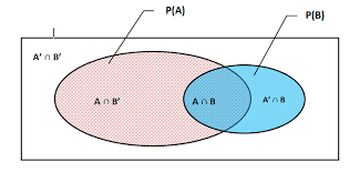
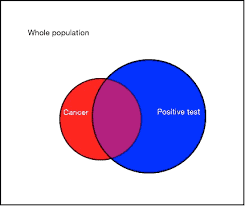
To formally state the Bayes theorem, let $B_{1}, B_{2}, \ldots, B_{k}$ be a set of mutually exclusive and exhaustive events and let $A$ be another event with positive probability (see illustration in Figure 4.1). The Bayes theorem states that for any $i, i=1, \ldots, k$, $$ P\left(B_{i} \mid A\right)=\frac{P\left(B_{i} \cap A\right)}{P(A)}=\frac{P\left(A \mid B_{i}\right) P\left(B_{i}\right)}{\sum_{j=1}^{k} P\left(A \mid B_{j}\right) P\left(B_{j}\right)} $$ Example 4.1. We can understand the theorem using a simple example. Consider a rare disease that is thought to occur in $0.1 \%$ of the population. Using a particular blood test a physician observes that out of the patients with disease $99 \%$ possess a particular symptom. Also assume that $1 \%$ of the population without the disease have the same symptom. A randomly chosen person from the population is blood tested and is shown to have the symptom. What is the conditional probability that the person has the disease?
Here $k=2$ and let $B_{1}$ be the event that a randomly chosen person has the disease and $B_{2}$ is the complement of $B_{1}$. Let $A$ be the event that a randomly chosen person has the symptom. The problem is to determine $P\left(B_{1} \mid A\right)$. We have $P\left(B_{1}\right)=0.001$ since $0.1 \%$ of the population has the disease, and $P\left(B_{2}\right)=0.999$. Also, $P\left(A \mid B_{1}\right)=0.99$ and $P\left(A \mid B_{2}\right)=0.01$. Now $$ \begin{aligned} P(\text { disease } \mid \text { symptom })=P\left(B_{1} \mid A\right) &=\frac{P\left(A \mid B_{1}\right) P\left(B_{1}\right)}{P\left(A \mid B_{1}\right) P\left(B_{1}\right)+P\left(A \mid B_{2}\right) P\left(B_{2}\right)} \ &=\frac{0.99 \times 0.001}{0.99 \times 0.001+0.999 \times 0.01} \ &=\frac{99}{99+999}=0.09 . \end{aligned} $$ The probability of disease given symptom here is very low, only $9 \%$, since the
disease is a very rare disease and there will be a large percentage of individuals in the population who have the symptom but not the disease, highlighted by the figure 999 as the second last term in the denominator above.
It is interesting to see what happens if the same person is found to have the same symptom in another independent blood test. In this case, the prior probability of $0.1 \%$ would get revised to $0.09$ and the revised posterior probability is given by: $$ P(\text { disease } \mid \text { twice positive })=\frac{0.99 \times 0.09}{0.99 \times 0.09+0.91 \times 0.01}=0.908 . $$ As expected, this probability is much higher since it combines the evidence from two independent tests. This illustrates an aspect of the Bayesian world view: the prior probability gets continually updated in the light of new evidence.
统计代写|贝叶斯统计代写beyesian statistics代考|Bayes theorem for random variables
The Bayes theorem stated above is generalized for two random variables instead of two events $A$ and $B_{i}$ ‘s as noted above. In the generalization, $B_{i}$ ‘s will be replaced by the generic parameter $\theta$ which we want to estimate and $A$ will be replaced by the observation random variable denoted by $Y$. Also, the probabilities of events will be replaced by the probability (mass or density) function of the argument random variable. Thus, $P\left(A \mid B_{i}\right)$ will be substituted by $f(y \mid \theta)$ where $f(\cdot$ ) denotes the probability (mass or density) function of the random variable $X$ given a particular value of $\theta$. The replacement for $P\left(B_{i}\right)$ is $\pi(\theta)$, which is the prior distribution of the unknown parameter $\theta$. If $\theta$ is
a discrete parameter taking only finite many, $k$ say, values, then the summation in the denominator of the above Bayes theorem will stay as it is since $\sum_{j=1}^{k} \pi\left(\theta_{j}\right)$ must be equal to 1 as the total probability. If, however, $\theta$ is a continuous parameter then the summation in the denominator of the Bayes theorem must be replaced by an integral over the range of $\theta$, which is generally taken as the whole of the real line.
The Bayes theorem for random variables is now stated as follows. Suppose that two random variables $Y$ and $\theta$ are given with probability density functions (pdfs) $f(y \mid \theta)$ and $\pi(\theta)$, then $$ \pi(\theta \mid y)=\frac{f(y \mid \theta) \pi(\theta)}{\int_{-\infty}^{\infty} f(y \mid \theta) \pi(\theta) d \theta},-\infty<\theta<\infty . $$ The probability distribution given by $\pi(\theta)$ captures the prior beliefs about the unknown parameter $\theta$ and is the prior distribution in the Bayes theorem. The posterior distribution of $\theta$ is given by $\pi(\theta \mid y)$ after observing the value $y$ of the random variable $Y$. We illustrate the theorem with the following example. Example 4.2. Binomial Suppose $Y \sim \operatorname{binomial}(n, \theta)$ where $n$ is known and we assume $\operatorname{Beta}(\alpha, \beta)$ prior distribution for $\theta$. Here the likelihood function is $$ f(y \mid \theta)=\left(\begin{array}{l} n \ y \end{array}\right) \theta^{y}(1-\theta)^{n-y} $$ for $0<\theta<1$. The function $f(y \mid \theta)$ is to be viewed as a function of $\theta$ for a given value of $y$, although its argument is written as $y \mid \theta$ instead of $\theta \mid y$. This is because we use the probability density function of $Y$, which is more widely known, and we avoid introducing further notation for the likelihood function e.g. $L(\theta ; y)$.
Suppose that the prior distribution is the beta distribution (A.22) having density $$ \pi(\theta)=\frac{1}{B(\alpha, \beta)} \theta^{\alpha-1}(1-\theta)^{\beta-1}, \quad 0<\theta<1 . $$
统计代写|贝叶斯统计代写beyesian statistics代考|Sequential updating of the posterior distribution
Consider the denominator in the posterior distribution. The denominator, given by, $\int_{-\infty}^{\infty} f(y \mid \theta) \pi(\theta) d \theta$ or $\int_{-\infty}^{\infty} f\left(y_{1}, \ldots, y_{n} \mid \theta\right) \pi(\theta) d \theta$ is free of the unknown parameter $\theta$ since $\theta$ is only a dummy in the integral, and it has been integrated out in the expression. The posterior distribution $\pi\left(\theta \mid y_{1}, \ldots, y_{n}\right)$ is to be viewed as a function of $\theta$ and the denominator is merely a constant. That is why, we often ignore the constant denominator and write the posterior distribution $\pi\left(\theta \mid y_{1}, \ldots, y_{n}\right)$ as $$ \pi\left(\theta \mid y_{1}, \ldots, y_{n}\right) \propto f\left(y_{1}, \ldots, y_{n} \mid \theta\right) \times \pi(\theta) $$ By noting that $f\left(y_{1}, \ldots, y_{n} \mid \theta\right)$ provides the likelihood function of $\theta$ and $\pi(\theta)$ is the prior distribution for $\theta$, we write: Posterior $\propto$ Likelihood $\times$ Prior. Hence we always know the posterior distribution up-to a normalizing constant. Often we are able to identify the posterior distribution of $\theta$ just by looking at the numerator as in the two preceding examples.
The structure of the Bayes theorem allows sequential updating of the posterior distribution. By Bayes theorem we “update” the prior belief $\pi(\theta)$ to $\pi(\theta \mid \mathbf{y})$. Note that $\pi\left(\theta \mid y_{1}\right) \propto f\left(y_{1} \mid \theta\right) \pi(\theta)$ and if $Y_{2}$ is independent of $Y_{2}$ given the parameter $\theta$, then: $$ \begin{aligned} \pi\left(\theta \mid y_{1}, y_{2}\right) & \propto & f\left(y_{2} \mid \theta\right) f\left(y_{1} \mid \theta\right) \pi(\theta) \ & \propto f\left(y_{2} \mid \theta\right) \pi\left(\theta \mid y_{1}\right) \end{aligned} $$ Thus, at the second stage of data collection, the first stage posterior distribution, $\pi\left(\theta \mid y_{1}\right)$ acts as the prior distribution to update our belief about $\theta$ after. Thus, the Bayes theorem shows how the knowledge about the state of nature represented by $\theta$ is continually modified as new data becomes available. There is another strong point that jumps out of this sequential updating. It is possible to start with a very weak prior distribution $\pi(\theta)$ and upon observing data sequentially the prior distribution gets revised to a stronger one, e.g. $\pi\left(\theta \mid y_{1}\right)$ when just one observation has been recorded – of course, assuming that data are informative about the unknown parameter $\theta$.
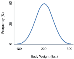
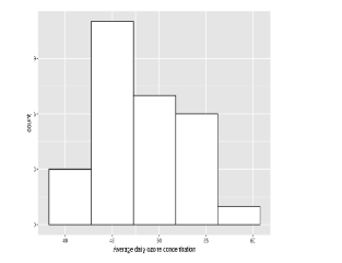
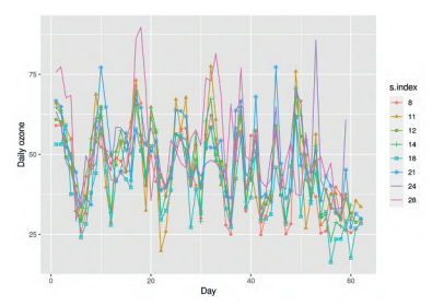
Recall the air pollution data set nysptime introduced in Section $1.3 .1$ which contains the daily maximum ozone concentration values at the 28 sites shown in Figure $1.1$ in the state of New York for the 62 days in July and August 2006. From this data set we have created a spatial data set, named nyspatial, which contains the average air pollution and the average values of the three covariates at the 28 sites. Figure $3.1$ provides a histogram for the response, average daily ozone concentration levels, at the 28 monitoring sites. The plot does not show a symmetric bell-shaped histogram but it does admit the possibility of a unimodal distribution for the response. The $R$ command used to draw the plot is given below:
The geom_histogram command has been invoked with a bin width argument of $4.5$. The shape of the histogram will change if a different bin width is supplied. As is well known, a lower value will provide a lesser degree of smoothing while a higher value will increase more smoothing by collapsing the number of classes. It is also possible to adopt a different scale, e.g. square root or logarithm, but we have not done so here to illustrate modeling on the original scale of the data. We shall explore different scales for the spatio-temporal version of this data set.
Figure $3.2$ provides a pair-wise scatter plot of the response against the three explanatory covariates: maximum temperature, wind speed and relative humidity. The diagonal panels in this plot provides kernel density estimates of the variables. This plot reveals that wind speed correlates the most with ozone levels at this aggregated average level. As is well known, see e.g. Sahu and Bakar (2012a), the maximum temperature also positively correlates with the ozone levels. Relative humidity is seen to have the least amount of correlation with ozone levels. This plot has been obtained using the commands.
统计代写|贝叶斯统计代写beyesian statistics代考|Exploring spatio-temporal point reference data
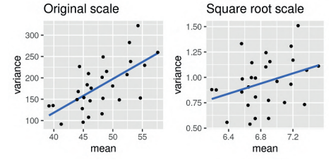
This section illustrates EDA methods with the nysptime data set in bmstdr. To decide the modeling scale Figure $3.5$ plots the mean against variance for each site on the original scale and also on the square root scale for the response. A stronger linear mean-variance relationship with a larger value of the slope for the superimposed regression line is observed on the original scale making this less suitable for modeling purposes. This is because in linear statistical modeling we often model the mean as a function of the available covariates and assume equal variance (homoscedasticity) for the residual differences between the observed and modeled values. A word of caution here is that the right panel does not show a complete lack of mean-variance relationship. However, we still prefer to model on the square root scale to stabilize the variance and in this case the predictions we make in Chapter 7 for ozone concentration values do not become negative.
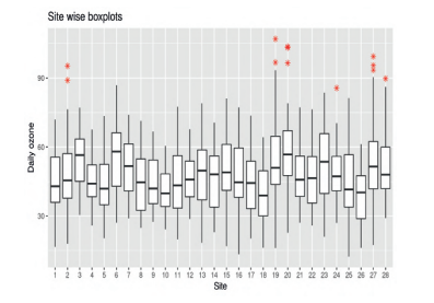
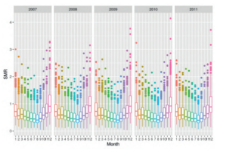
Temporal variations are illustrated in Figures $3.6$ for all 28 sites and in Figure $3.8$ for the 8 sites which have been used for model validation purposes in Chapters 6 and 7. Figure $3.7$ shows variations of ozone concentration values for the 28 monitoring sites. Suspected outliers, data values which are at a distance beyond $1.5$ times the inter quartile range from the whiskers, are plotted as red stars. Such high values of ground level ozone pollution are especially harmful to humans.
统计代写|贝叶斯统计代写beyesian statistics代考|Exploring areal Covid-19 case and death data
This section explores the Covid-19 mortality data introduced in Section 1.4.1. The bmstdr data frame engtotals contains aggregated number of deaths along with other relevant information for analyzing and modeling this data set. The data frame object engdeaths contains the death numbers by the 20 weeks from March 13 to July 31,2020 . These two data sets will be used to illustrate spatial and spatio-temporal modeling for areal data in Chapter 10 . Typical such areal data are represented by a choropleth map which uses shades of color or grey scale to classify values into a few broad classes, like a histogram. Two choropleth maps have been provided in Figure $1.9$.
For the engtotals data set the minimum and maximum number of deaths were 4 and 1223 respectively for the City of London (a very small borough within greater London with population 9721) and Birmingham with population $1,141,816$ in 2019 . However, the minimum and maximum death rates per 100,000 were $10.79$ and $172.51$ respectively for Hastings (in the South East) and Hertsmere (near Watford in greater London) respectively.
Calculation of the Moran’s I for number and rate of deaths is performed by using the moran .me function in the library spdep. This function requires the spatial adjacency matrix in a list format, which is obtained by the poly2nb and nb2listw functions in the spdep library. The Moran’s I statistics for the raw observed death numbers and the rate are found to be $0.34$ and $0.45$ respectively both with a p-value smaller than $0.001$ for the null hypothesis of no spatial autocorrelation. The permutation tests in statistics randomly permute the observed data and then calculates the relevant statistics for a number of replications. These replicate values of the statistics are used to approximate the null distribution of the statistics against which the observed value of the statistics for the observed data is compared and an approximate $\mathrm{p}$-value is found. The tests with Geary’s $\mathrm{C}$ statistics gave a $\mathrm{p}$-value of less than $0.001$ for the death rate per 100,000 but the p-value was higher, $0.025$, for the un-adjusted observed Covid death numbers. Thus, the higher degree of spatial variation in the death rates has been successfully detected by the Geary’s statistics. The code lines to obtain these results are given below.
统计代写|贝叶斯统计代写Bayesian statistics代考|Exploratory data analysis methods
已使用 bin 宽度参数调用 geom_histogram 命令4.5. 如果提供不同的 bin 宽度,直方图的形状将发生变化。众所周知,较低的值将提供较小程度的平滑,而较高的值将通过折叠类的数量来增加更多的平滑度。也可以采用不同的尺度,例如平方根或对数,但我们在这里没有这样做来说明对数据原始尺度的建模。我们将探索该数据集时空版本的不同尺度。
数字3.2提供了对三个解释性协变量的响应的成对散点图:最高温度、风速和相对湿度。该图中的对角线面板提供了变量的核密度估计。该图显示,风速与此聚合平均水平的臭氧水平最相关。众所周知,参见例如 Sahu 和 Bakar (2012a),最高温度也与臭氧水平正相关。相对湿度被认为与臭氧水平的相关性最小。该图是使用命令获得的。
统计代写|贝叶斯统计代写beyesian statistics代考|Exploring spatio-temporal point reference data
The keyword CAR in CAR models stands for Conditional AutoRegression. This concept is often used in the context of modeling areal data which can be either discrete counts or continuous measurements. However, the CAR models are best described using the assumption of the normal distribution although CAR models for discrete data are also available. In our Bayesian modeling for areal data CAR models are used as prior distributions for spatial effects defined on the areal units. This justifies our treatment of CAR models using the normal distribution assumption.
Assume that we have areal data $Y_{i}$ for the $n$ areal units. The conditional in CAR stands for conditioning based on all the others. For example, we like to think of $Y_{1}$ given $Y_{2}, \ldots, Y_{n}$. The AutoRegression terms stand for regression on itself (auto). Putting these concepts together the CAR models are based on regression of each $Y_{i}$ conditional on the others $Y_{j}$ for $j=1, \ldots n$ but with
$j \neq i$. The constraint $j \neq i$ makes sure that we do not use $Y_{i}$ to define the distribution of $Y_{i}$. Thus, a typical CAR model will be written as $$ Y_{i} \mid y_{j}, j \neq i \sim N\left(\sum_{j} b_{i j} y_{j}, \sigma_{i}^{2}\right) $$ where the $b_{i j}$ ‘s are presumed to be the regression coefficients for predicting $Y_{i}$ based on all the other $Y_{j}$ ‘s. The full distributional specification for $\mathbf{Y}=\left(Y_{1}, \ldots, Y_{n}\right)$ comes from the independent product specification of the distributions $(2.6)$ for each $i=1, \ldots, n$. There are several key points and concepts that we now discuss to understand and we present those below as a bulleted list.
The models (2.6) can be equivalently rewritten as $$ \mathbf{Y}=B \mathbf{Y}+\epsilon $$ where $\epsilon=\left(\epsilon_{1}, \ldots, \epsilon_{n}\right)$ is a multivariate normal error distribution with zero means. The appearance of $\mathbf{Y}$ on the right hand side of the above emphasizes the keywords AutoRegression in CAR.
The CAR specification defines a valid multivariate normal probability distribution for $\mathbf{Y}$ under the additional conditions $$ \frac{b_{i j}}{\sigma_{i}^{2}}=\frac{b_{j i}}{\sigma_{j}^{2}}, i, j=1, \ldots, n $$ which are required to ensure that the inverse covariance matrix $\Sigma^{-1}$ in (A.24), is symmetric.
统计代写|贝叶斯统计代写beyesian statistics代考|Point processes
Spatial point pattern data arise when an event of interest, e.g. outbreak of a disease, e.g. Covid-19, occurs at random locations inside a study region of interest, $\mathbb{D}$. Often the main interest in such a case lies in discovering any explainable or non-random pattern in a scatter plot of the data locations. Absence of any regular pattern in the data locations is said to correspond to the model of complete spatial randomness, CSR, which is also called a Poisson process. Under CSR, the number of points in any given sub-region will follow the Poisson distribution with a parameter value proportional to the area of the sub-region. Often, researchers are interested in rejecting the model of CSR in favor of their own theories of the evolution or clustering of the points. In this context the researchers have to decide what all type of clustering may possibly explain the clustering pattern of points and which one of those provides the “best” fit to the observed data. There are other obvious investigations to make, for example, are there any suitable covariates which may explain the pattern? To illustrate, a lack of trees in many areas in a city may be explained by a layer of built environment.
Spatio-temporal point process data are naturally found in a number of disciplines, including (human or veterinary) epidemiology where extensive datasets are also becoming more common. One important distinction in practice is between processes defined as a discrete-time sequence of spatial point processes, or as a spatially and temporally continuous point process. See the books by Diggle (2014) and Møller and Waagepetersen (2003) for many examples and theoretical developments.
统计代写|贝叶斯统计代写beyesian statistics代考|Conclusion
The main purpose of this chapter has been to introduce the key concepts we need to pursue spatio-temporal modeling in the later chapters. Spatiotemporal modeling, as any other substantial scientific area of research, has its own unique set of keywords and concept dictionary. Not knowing some of these is a barrier to fully understanding, or more appropriately appreciating, what is going on under the hood of modeling equations. Thus, this chapter plugs the knowledge gap a reader may have regarding the typical terminology used while modeling.
It has not been possible to keep the chapter completely notation free. Notations have been introduced to keep the rigor in presentation and also as early and unique reference points for many key concepts assumed in the later chapters. For example, the concepts of Gaussian Process (GP), Kriging, internal and external standardization are defined without the data application overload. Of course, it is possible to skip reading of this chapter until a time when the reader is confronted with an un-familiar jargon.
CAR 模型中的关键字 CAR 代表 Conditional AutoRegression。这个概念通常用于建模区域数据的上下文中,这些数据可以是离散计数或连续测量。然而,CAR 模型最好使用正态分布的假设来描述,尽管也可以使用离散数据的 CAR 模型。在我们对面积数据的贝叶斯建模中,CAR 模型被用作在面积单位上定义的空间效应的先验分布。这证明了我们使用正态分布假设处理 CAR 模型的合理性。
统计代写|贝叶斯统计代写Bayesian statistics代考|Measures of spatial association for areal data
统计代写|贝叶斯统计代写beyesian statistics代考|Measures of spatial association for areal data
Exploration of areal spatial data requires definition of a sense of spatial distance between all the constituting areal units within the data set. This measure of distance is parallel to the distance $d$ between any two point referenced spatial locations discussed previously in this chapter. A blank choropleth map, e.g. Figure $1.12$ without the color gradients, provides a quick visual measure of spatial distance, e.g. California, Nevada and Oregon in the west coast are spatial neighbors but they are quite a long distance away from Pennsylvania, New York and Connecticut in the east coast. More formally, the concept of spatial distance for areal data is captured by what is called a neighborhood, or a proximity, or an adjacency, matrix. This is essentially a matrix where each of its entry is used to provide information on the spatial relationship between each possible pair of the areal units in the data set.
The proximity matrix, denoted by $W$, consists of weights which are used to represent the strength of spatial association between the different areal units. Assuming that there are $n$ areal units, the matrix $W$ is of the order $n \times n$ where each of its entry $w_{i j}$ contains the strength of spatial association between the units $i$ and $j$, for $i, j=1, \ldots, n$. Customarily, wii is set to 0 for each $i=1, \ldots, n$. Commonly, the weights $w_{i j}$ for $i \neq j$ are chosen to be binary where it is assigned the value 1 if units $i$ and $j$ share a common boundary and 0 otherwise. This proximity matrix can readily be formed just by inspecting a choropleth map, such as the one in Figure 1.12. However, the weighting function can instead be designed so as to incorporate other spatial information, such as the distances between the areal units. If required, additional proximity matrices can be defined for different orders, whereby the order dictates the proximity of the areal units. For instance we may have a first order proximity matrix representing the direct neighbors for an areal unit,
a second order proximity matrix representing the neighbors of the first order areal units and so on. These considerations will render a proximity matrix, which is symmetric, i.e. $w_{i j}=w_{j i}$ for all $i$ and $j$.
The weighting function $w_{i j}$ can be standardized by calculating a new proximity matrix given by $\tilde{w}{i j}=w{i j} / w_{i+}$ where $w_{i+}=\sum_{j=1}^{n} w_{i j}$, so that each areal unit is given a sense of “equality” in any statistical analysis. However, in this case the new proximity matrix may not remain symmetric, i.e. $\tilde{w}{i j}$ may or may not equal $\tilde{w}{j i}$ for all $i$ and $j$.
When working with grid based areal data, where the proximity matrix is defined based on touching areal units, it is useful to specify whether “queen” or “rook”, in a game of chess, based neighbors are being used. In the $R$ package spdep, “queen” based neighbors refer to any touching areal units, whereas “rook” based neighbors use the stricter criteria that both areal units must share an edge (Bivand, 2020).
There are two popular measures of spatial association for areal data which together serve as parallel to the concept of the covariance function, and equivalently variogram, defined earlier in this chapter. The first of these two measures is the Moran’s $I$ (Moran, 1950) which acts as an adaptation of Pearson’s correlation coefficient and summarizes the level of spatial autocorrelation present in the data. The measure $I$ is calculated by comparing each observed area $i$ to its neighboring areas using the weights, $w_{i j}$, from the proximity matrix for all $j=1, \ldots, n$. The formula for Moran’s $I$ is written as: $$ I=\frac{n}{\sum_{i \neq j} w_{i j}} \frac{\sum_{i=1}^{n} \sum_{j=1}^{n} w_{i j}\left(Y_{i}-\bar{Y}\right)\left(Y_{j}-\bar{Y}\right)}{\sum_{i=1}^{n}\left(Y_{i}-\bar{Y}\right)^{2}}, $$ where $Y_{i}, i=1, \ldots, n$ is the random sample from the $n$ areal units and $\bar{Y}$ is the sample mean. It can be shown that $I$ lies in the interval $[-1,1]$, and its sampling variance can be found, see e.g. Section $4.1$ in Banerjee et al. (2015) so that an asymptotic test can be performed by appealing to the central limit theorem. For small values of $n$ there are permutation tests which compares the observed value of $I$ to a null distribution of the test statistic $I$ obtained by simulation. We shall illustrate these with a real data example in Section 3.4. An alternative to the Moran’s $I$ is the Geary’s $C$ (Geary, 1954) which also measures spatial autocorrelation present in the data. The Geary’s $C$ is given by $$ C=\frac{(n-1)}{2 \sum_{i \neq j} w_{i j}} \frac{\sum_{i=1}^{n} \sum_{j=1}^{n} w_{i j}\left(Y_{i}-Y_{j}\right)^{2}}{\sum_{i=1}^{n}\left(Y_{i}-\bar{Y}\right)^{2}} . $$ The measure $C$ being the ratio of two weighted sum of squares is never negative. It can be shown that $E(C)=1$ under the assumption of no spatial association. Small values of $C$ away from the mean 1 indicate positive spatial association. An asymptotic test can be performed but the speed of convergence to the limiting null distribution is expected to be very slow since it is a ratio of weighted sum of squares. Monte Carlo permutation tests can be performed and those will be illustrated in Section $3.4$ with a real data example.
统计代写|贝叶斯统计代写beyesian statistics代考|Internal and external standardization for areal data
Internal and external standardization are two oft-quoted keywords in areal data modeling, especially in disease mapping where rates of a disease over different geographical (areal) units are compared. These two are now defined along with other relevant key words. To facilitate the comparison often we aim to understand what would have happened if all the areal units had the same uniform rate. This uniform rate scenario serves as a kind of a null hypothesis of “no spatial clustering or association”. Disease incidence rates in excess or in deficit relative to the uniform rate is called the relative risk. Relative risk is often expressed as a ratio where the denominator corresponds to the standard dictated by the above null hypothesis. Thus, a relative risk of $1.2$ will imply $20 \%$ increased risk relative to the prevailing standard rate. The relative risk can be associated with a particular geographical areal unit or even for the whole study domain when the standard may refer to an absence of the disease. Statistical models are often postulated for the relative risk for the ease of interpretation.
Return to the issue of comparison of disease rates relative to the uniform rate. Often in practical data modeling situation, the counts of number of individuals over different geographies and other categories, e.g. sex and ethnicity, are available. Standardization, internal and external, is a process by which we obtain the corresponding counts of diseased individuals under the assumption of the null hypothesis of uniform disease rates being true. We now introduce the notation $n_{i}$, for $i=1, \ldots, k$ being the total number of individuals in region $i$ and $y_{i}$ being the observed number of individuals with the disease, often called cases, in region $i$. Under the null hypothesis $$ \bar{r}=\frac{\sum_{i=1}^{k} y_{i}}{\sum_{i=1}^{k} n_{i}} $$ will be an estimate of the uniform disease rate. As a result, $$ E_{i}=n_{i} \bar{r} $$ will be the expected number of individuals with the disease in region $i$ if the null hypothesis of uniform disease rate is true. Note that $\sum_{i=1}^{k} E_{i}=\sum_{i=1}^{k} y_{i}$ so that the total number of observed and expected cases are same. Note that to find $E_{i}$ we used the observations $y_{i}, i=1, \ldots, k$. This process of finding the $E_{i}$ ‘s is called internal standardization. The word internal highlights the use of the data itself to perform the standardization.
The technique of internal standardization is appealing to the analysts since no new external data are needed for the purposes of modeling and analysis. However, this technique is often criticized since in the modeling process $E_{i}$ ‘s are treated as fixed values when in reality these are functions of the random observations $y_{i}$ ‘s of the associated random variables $Y_{i}$ ‘s. Modeling of the $Y_{i}$ ‘s while treating the $E_{i}$ s as fixed is the unsatisfactory aspect of this strategy. To overcome this drawback the concept of external standardization is often used and this is what is discussed next.
Observed spatially referenced data will not be smooth in general due to the presence of noise and many other factors, such as data being observed at a
coarse irregular spatial resolution where observation locations are not on a regular grid. Such irregular variations hinder making inference regarding any dominant spatial pattern that may be present in the data. Hence researchers often feel the need to smooth the data to discover important discernible spatial trend from the data. Statistical modeling, as proposed in this book, based on formal coherent methods for fitting and prediction, is perhaps the best formal method for such smoothing needs. However, researchers often use many non-rigorous off-the shelf methods for spatial smoothing either as exploratory tools demonstrating some key features of the data or more dangerously for making inference just by “eye estimation” methods. Our view in this book is that we welcome those techniques primarily as exploratory data analysis tools but not as inference making tools. Model based approaches are to be used for smoothing and inference so that the associated uncertainties of any final inferential product may be quantified fully.
For spatially point referenced data we briefly discuss the inverse distance weighting (IDW) method as an example method for spatial smoothing. There are many other methods based on Thiessen polygons and crude application of Kriging (using ad-hoc estimation methods for the unknown parameters). These, however, will not be discussed here due to their limitations in facilitating rigorous model based inference.
To perform spatial smoothing, the IDW method first prepares a fine grid of locations covering the study region. The IDW method then performs interpolation at each of those grid locations separately. The formula for interpolation is a weighted linear function of the observed data points where the weight for each observation is inversely proportional to the distance between the observation and interpolation locations. Thus to predict $Y\left(\mathrm{~s}{0}\right)$ at location $\mathbf{s}{0}$ the IDW method first calculates the distance $d_{i 0}=\left|\mathbf{s}{i}-\mathbf{s}{0}\right|$ for $i=1, \ldots, n$. The prediction is now given by: $$ \hat{Y}\left(\mathbf{s}{0}\right)=\frac{1}{\sum{i=1}^{n} \frac{1}{d_{i 0}}} \sum_{i=1}^{n} \frac{y\left(\mathbf{s}{i}\right)}{d{i 0}} $$ Variations in the basic IDW methods are introduced by replacing $d_{i 0}$ by the $p$ th power, $d_{i 0}^{p}$ for some values of $p>0$. The higher the value of $p$, the quicker the rate of decay of influence of the distant observations in the interpolation. Note that it is not possible to attach any uncertainty measure to the individual predictions $Y\left(\mathbf{s}{0}\right)$ since a joint model has not been specified for the random vector $Y\left(\mathbf{s}{0}\right), Y\left(\mathbf{s}{1}\right), \ldots, Y\left(\mathbf{s}{n}\right)$. However, in practice, an overall error rate such as the root mean square prediction error can be calculated for set aside validation data sets. Such an overall error rate will fail to ascertain uncertainty for prediction at an individual location.
There are many methods for smoothing areal data as well. One such method is inspired by what are known as conditionally auto-regressive (CAR) models which will be discussed more formally later in Section 2.14. In implementing this method we first need to define a neighborhood structure.
统计代写|贝叶斯统计代写Bayesian statistics代考|Measures of spatial association for areal data
A particular covariance structure must be assumed for the $Y\left(\mathbf{s}{i}, t\right)$ process. The pivotal space-time covariance function is defined as $$ C\left(\mathbf{s}{1}, \mathbf{s}{2} ; t{1}, t_{2}\right)=\operatorname{Cov}\left[Y\left(\mathbf{s}{1}, t{1}\right), Y\left(\mathbf{s}{2}, t{2}\right)\right] . $$ The zero mean spatio-temporal process $Y(s, t)$ is said to be covariance stationary if $$ C\left(\mathbf{s}{1}, \mathbf{s}{2} ; t_{1}, t_{2}\right)=C\left(\mathbf{s}{1}-\mathbf{s}{2} ; t_{1}-t_{2}\right)=C(d ; \tau) $$
where $d=\mathbf{s}{1}-\mathbf{s}{2}$ and $\tau=t_{1}-t_{2}$. The process is said to be isotropic if $$ C(d ; \tau)=C(|d| ;|\tau|), $$ that is, the covariance function depends upon the separation vectors only through their lengths ||$d||$ and $|\tau|$. Processes which are not isotropic are called anisotropic. In the literature isotropic processes are popular because of their simplicity and interpretability. Moreover, there is a number of simple parametric forms available to model those.
A further simplifying assumption to make is the assumption of separability; see for example, Mardia and Goodall (1993). Separability is a concept used in modeling multivariate spatial data including spatio-temporal data. A separable covariance function in space and time is simply the product of two covariance functions one for space and the other for time. The process $Y(\mathbf{s}, t)$ is said to be separable if $$ \left.C(|d| ;|\tau|)=C_{s}(|d|)\right) C_{t}(|\tau|) . $$ Now suitable forms for the functions $C_{s}(\cdot)$ and $C_{t}(\cdot)$ are to be assumed. A very general choice is to adopt the Matèrn covariance function introduced before. There is a growing literature on methods for constructing non-separable and non-stationary spatio-temporal covariance functions that are useful for modeling. See for example, Gneiting (2002) who develops a class of nonseparable covariance functions. A simple example is: $$ C(|d| ;|\tau|)=(1+|\tau|)^{-1} \exp \left{-| d|| /(1+|\tau|)^{\beta / 2}\right}, $$ where $\beta \in[0,1]$ is a space-time interaction parameter. For $\beta=0,(2.3)$ provides a separable covariance function. The other extreme case at $\beta=1$ corresponds to a totally non-separable covariance function. Figure $2.3$ plots this function for four different values: $0,0.25,0.5$ and 1 of $\beta$. There are some discernible differences between the functions can be seen for higher distances at the top right corner of each plot. However, it is true that it is not easy to describe the differences, and it gets even harder to see differences in model fits. The paper by Gneiting (2002) provides further descriptions of non-separable covariance functions.
There are other ways to construct non-separable covariance functions, for example, by mixing more than one spatio-temporal processes, see e.g. Sahu et al. (2006) or by including a further level of hierarchy where the covariance matrix obtained using $C(|d| ;|\tau|)$ follows a inverse-Wishart distribution centred around a separable covariance matrix. Section $8.3$ of the book by Banerjee et al. (2015) also lists many more strategies. For example, Schmidt and O’Hagan (2003) construct non-stationary spatio-temporal covariance structure via deformations.
统计代写|贝叶斯统计代写beyesian statistics代考|Kriging or optimal spatial prediction
The jargon “Kriging” refers to a form of spatial prediction at an unobserved location based on the observed data. That it is a popular method is borne by the fact that “Kriging” is verbification of a method of spatial prediction named after its inventor D.G. Krige, a South African mining engineer. Kriging solves the problem of predicting $Y(\mathbf{s})$ at a new location $\mathbf{s}{0}$ having observed data $y\left(\mathbf{s}{1}\right), \ldots, y\left(\mathbf{s}_{n}\right)$.
Classical statistical theory based on squared error loss function in prediction will yield the sample mean $\bar{y}$ to be the optimal predictor for $Y\left(\mathbf{s}{0}\right)$ if spatial dependency is ignored between the random variables $Y\left(\mathbf{s}{0}\right), Y\left(\mathbf{s}{1}\right), \ldots, Y\left(\mathbf{s}{n}\right)$. Surely, because of the Tobler’s law, the prediction for $Y\left(\mathbf{s}{0}\right)$ will be improved if instead spatial dependency is taken into account. The observations nearer to the prediction location, $\mathbf{s}{0}$, will receive higher weights in the prediction formula than the observations further apart. So, now the question is how do we determine these weights? Kriging provides the answer. In order to proceed further we assume that $Y(\mathbf{s})$ is a GP, although some of the results we discuss below also hold in general without this assumption. In order to perform Kriging it is assumed that the best linear unbiased predictor with weights $l_{i}, \hat{Y}\left(\mathrm{~s}{0}\right)$, is of the form $\sum{i=1}^{n} \ell_{i} Y\left(\mathbf{s}{i}\right)$ and dependence between the $Y\left(\mathbf{s}{0}\right), Y\left(\mathbf{s}{1}\right), \ldots, Y\left(\mathbf{s}{n}\right)$ is described by a covariance function, $C(d \mid \psi)$, of the distance $d$ between any two locations as defined above in this chapter. The Kriging weights are easily determined by evaluating the conditional mean of $Y\left(\mathbf{s}{0}\right)$ given the observed values $y\left(\mathbf{s}{1}\right), \ldots, y\left(\mathbf{s}{n}\right)$. These weights are “optimal” in the same statistical sense that the mean $E(X)$ minimizes the expected value of the squared error loss function, i.e. $E(X-a)^{2}$ is minimized at $a=$ $E(X)$. Here we take $X$ to be the conditional random variable $Y\left(\mathrm{~s}{0}\right)$ given $y\left(\mathbf{s}{1}\right), \ldots, y\left(\mathbf{s}{n}\right) .$
The actual values of the optimal weights are derived by partitioning the mean vector, $\boldsymbol{\mu}{n+1}$ and the covariance matrix, $\Sigma$, of $Y\left(\mathbf{s}{0}\right), Y\left(\mathbf{s}{1}\right), \ldots, Y\left(\mathbf{s}{n}\right)$ as follows. Let $$ \boldsymbol{\mu}{n+1}=\left(\begin{array}{c} \mu{0} \ \boldsymbol{\mu} \end{array}\right), \quad \Sigma=\left(\begin{array}{cc} \sigma_{00} & \Sigma_{01} \ \Sigma_{10} & \Sigma_{11} \end{array}\right) $$ where $\boldsymbol{\mu}$ is the vector of the means of $\mathbf{Y}=\left(Y\left(\mathbf{s}{1}\right), \ldots, Y\left(\mathbf{s}{n}\right)\right)^{\prime} ; \sigma_{00}=$ $\operatorname{Var}\left(Y\left(\mathbf{s}{0}\right)\right) ; \Sigma{01}=\Sigma_{1,0}^{\prime}=\operatorname{Cov}\left(\begin{array}{c}Y\left(\mathbf{s}{0}\right) \ \mathbf{Y}{1}\end{array}\right) ; \Sigma_{11}=\operatorname{Var}\left(\mathbf{Y}{1}\right)$. Now standard multivariate normal distribution theory tells us that $$ Y\left(\mathbf{s}{0}\right) \mid \mathbf{y} \sim N\left(\mu_{0}+\Sigma_{01} \Sigma_{11}^{-1}(\mathbf{y}-\boldsymbol{\mu}), \sigma_{00}-\Sigma_{01} \Sigma_{11}^{-1} \Sigma_{10}\right) . $$ In order to facilitate a clear understanding of the underlying spatial dependence on Kriging we assume a zero-mean GP, i.e. $\boldsymbol{\mu}{\mathrm{n}+1}=\mathbf{0}$. Now we have $E\left(Y\left(\mathbf{s}{0}\right) \mid \mathbf{y}\right)=\Sigma_{01} \Sigma_{11}^{-1} \mathbf{y}$ and thus we see that the optimal Kriging weights are particular functions of the assumed covariance function. Note that the weights
do not depend on the underlying common spatial variance as that is canceled in the product $\Sigma_{01} \Sigma_{11}^{-1}$. However, the spatial variance will affect the accuracy of the predictor since $\operatorname{Var}\left(Y\left(\mathbf{s}{0}\right) \mid \mathbf{y}\right)=\sigma{00}-\Sigma_{01} \Sigma_{11}^{-1} \Sigma_{10}$.
It is interesting to note that Kriging is an exact predictor in the sense that $E\left(Y\left(\mathbf{s}{i}\right) \mid \mathbf{y}\right)=y\left(\mathbf{s}{i}\right)$ for any $i=1, \ldots, n$. It is intuitively clear why this result will hold. This is because a random variable is an exact predictor of itself. Mathematically, this can be easily proved using the definition of inverse of an matrix. To elaborate further, suppose that $$ \Sigma=\left(\begin{array}{c} \Sigma_{1}^{\prime} \ \Sigma_{2}^{\prime} \ \vdots \ \Sigma_{n}^{\prime} \end{array}\right) $$ where $\Sigma_{i}^{\prime}$ is a row vector of dimension $n$. Then the result $\Sigma \Sigma^{-1}=I_{n}$ where $I_{n}$ is the identity matrix of order $n$, implies that $\Sigma_{i} \Sigma^{-1}=\mathbf{a}{i}$ where the $i$ th element of $\mathbf{a}{i}$ is 1 and all others are zero.
The above discussion, with the simplified assumption of a zero mean GP, is justified since often in practical applications we only assume a zero-mean GP as a prior distribution. The mean surface of the data (or their transformations) is often explicitly modeled by a regression model and hence such models will contribute to determine the mean values of the predictions. In this context we note that in a non-Bayesian geostatistical modeling setup there are various flavors of Kriging such as simple Kriging, ordinary Kriging, universal Kriging, co-Kriging, intrinsic Kriging, depending on the particular assumption of the mean function. In our Bayesian inference set up such flavors of Kriging will automatically ensue since Bayesian inference methods are automatically conditioned on observed data and the explicit model assumptions.
统计代写|贝叶斯统计代写beyesian statistics代考|Autocorrelation and partial autocorrelation
A study of time series for temporally correlated data will not be complete without the knowledge of autocorrelation. Simply put, autocorrelation means correlation with itself at different time intervals. The time interval is technically called the lag in the time series literature. For example, suppose $Y_{t}$ is a time series random variable where $t \geq 1$ is an integer. The autocorrelation at lag $k(\geq 1)$ is defined as $\rho_{k}=\operatorname{Cor}\left(Y_{t+k}, Y_{t}\right)$. It is obvious that the autocorrelation at lag $k=0, \rho_{0}$, is one. Ordinarily, $\rho_{k}$ decreases as $k$ increases just as the spatial correlation decreases when the distance between two locations increases. Viewed as a function of the lag $k, \rho_{k}$ is called the autocorrelation function, often abbreviated as ACF.
Sometimes high autocorrelation at any lag $k>1$ persists because of high correlation between $Y_{t+k}$ and the intermediate time series, $Y_{t+k-1}, \ldots, Y_{t+1}$. The partial autocorrelation at lag $k$ measures the correlation between $Y_{t+k}$ and $Y_{t}$ after removing the autocorrelation at shorter lags. Formally, partial autocorrelation is defined as the conditional autocorrelation between $Y_{t+k}$ and $Y_{t}$ given the values of $Y_{t+k-1}, \ldots, Y_{t+1}$. The partial correlation can also be easily explained with the help of multiple regression. To remove the effects of intermediate time series $Y_{t+k-1}, \ldots, Y_{t+1}$ one considers two regression models: one $Y_{t+k}$ on $Y_{t+k-1}, \ldots, Y_{t+1}$ and the other $Y_{t}$ on $Y_{t+k-1}, \ldots, Y_{t+1}$. The simple correlation coefficient between two sets of residuals after fitting the two regression models is the partial auto-correlation at a given lag $k$. To learn more the interested reader is referred to many excellent introductory text books on time series such as the one by Chatfield (2003).
上述讨论,以及零均值 GP 的简化假设是合理的,因为在实际应用中,我们通常只假设零均值 GP 作为先验分布。数据的平均表面(或其转换)通常由回归模型明确建模,因此此类模型将有助于确定预测的平均值。在这种情况下,我们注意到在非贝叶斯地统计建模设置中,有各种风格的克里金法,例如简单克里金法、普通克里金法、通用克里金法、协同克里金法、内在克里金法,具体取决于均值函数的特定假设。在我们的贝叶斯推理设置中,由于贝叶斯推理方法会自动以观察到的数据和明确的模型假设为条件,因此会自动出现这种风格的克里金法。
统计代写|贝叶斯统计代写beyesian statistics代考|Autocorrelation and partial autocorrelation