标签: GR 5263

统计代写|金融统计代写Mathematics with Statistics for Finance代考|NORMAL DISTRIBUTION

如果你也在 怎样代写金融统计Mathematics with Statistics for Finance G1GH这个学科遇到相关的难题,请随时右上角联系我们的24/7代写客服。

金融统计描述了应用数学和数学模型来解决金融问题。它有时被称为定量金融,金融工程,和计算金融。

statistics-lab™ 为您的留学生涯保驾护航 在代写金融统计Mathematics with Statistics for Finance G1GH方面已经树立了自己的口碑, 保证靠谱, 高质且原创的统计Statistics代写服务。我们的专家在代写金融统计Mathematics with Statistics for Finance G1GH方面经验极为丰富,各种代写金融统计Mathematics with Statistics for Finance G1GH相关的作业也就用不着说。

我们提供的金融统计Mathematics with Statistics for Finance G1GH及其相关学科的代写,服务范围广, 其中包括但不限于:

  • Statistical Inference 统计推断
  • Statistical Computing 统计计算
  • Advanced Probability Theory 高等楖率论
  • Advanced Mathematical Statistics 高等数理统计学
  • (Generalized) Linear Models 广义线性模型
  • Statistical Machine Learning 统计机器学习
  • Longitudinal Data Analysis 纵向数据分析
  • Foundations of Data Science 数据科学基础
统计代写|金融统计代写Mathematics with Statistics for Finance代考|NORMAL DISTRIBUTION

统计代写|金融统计代写Mathematics with Statistics for Finance代考|NORMAL DISTRIBUTION

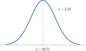
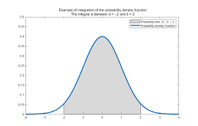
The normal distribution is probably the most widely used distribution in statistics, and is extremely popular in finance. The normal distribution occurs in a large number of settings, and is extremely easy to work with.

In popular literature, the normal distribution is often referred to as the bell curve because of the shape of its probability density function.

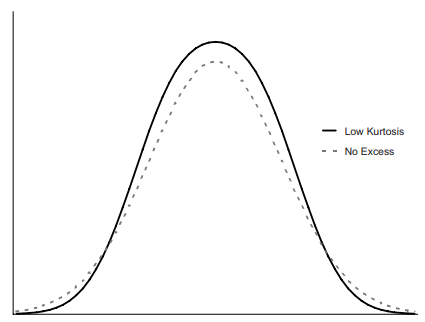
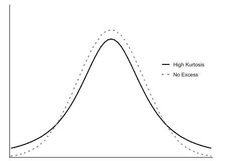
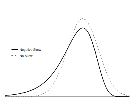
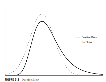
The probability density function of the normal distribution is symmetrical, with the mean and median coinciding with the highest point of the PDF. Because it is symmetrical, the skew of a normal distribution is always zero. The kurtosis of a normal distribution is always 3 . By definition, the excess kurtosis of a normal distribution is zero.

In some fields it is more common to refer to the normal distribution as the Gaussian distribution, after the famous German mathematician Johann Gauss, who is credited with some of the earliest work with the distribution. It is not the case that one name is more precise than the other as with mean and average. Both normal distribution and Gaussian distribution are acceptable terms.

For a random variable $X$, the probability density function for the normal distribution is:
$$
f(x)=\frac{1}{\sigma \sqrt{2 \pi}} e^{-\frac{1}{2}\left(\frac{x-\beta}{\sigma}\right)^{2}}
$$
The distribution is described by two parameters, $\mu$ and $\sigma ; \mu$ is the mean of the distribution and $\sigma$ is the standard deviation. We leave the proofs of these statements for the exercises at the end of the chapter.

Rather than writing out the entire density function, when a variable is normally distributed it is the convention to write:
$$
X \sim N\left(\mu, \sigma^{2}\right)
$$

This would be read ” $X$ is normally distributed with a mean of $\mu$ and variance of $\sigma^{2}$ “

One reason that normal distributions are easy to work with is that any linear combination of independent normal variables is also normal. If we have two normally distributed variables, $X$ and $Y$, and two constants, $a$ and $b$, then $Z$ is also normally distributed:
$$
Z=a X+b Y \text { s.t. } Z \sim N\left(a \mu_{X}+b \mu_{Y}, a^{2} \sigma_{X}^{2}+b^{2} \sigma_{Y}^{2}\right)
$$
This is very convenient. For example, if the log returns of individual stocks are normally distributed, then the average return of those stocks will also be normally distributed.

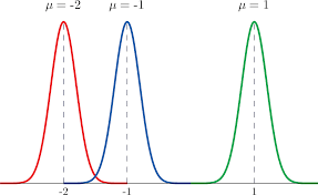
When a normal distribution has a mean of zero and a standard deviation of one, it is referred to as a standard normal distribution.
$$
\phi=\frac{1}{\sqrt{2 \pi}} e^{-\frac{1}{2} x^{2}}
$$
It is the convention to denote the standard normal PDF by $\phi$, and the cumulative standard normal distribution by $\Phi$.

Because a linear combination of normal distributions is also normal, standard normal distributions are the building blocks of many financial models. To get a normal variable with a standard deviation of $\sigma$ and a mean of $\mu$, we simply multiply the standard normal variable by $\sigma$ and add $\mu$.
$$
X=\mu+\sigma \phi \Rightarrow X \sim N\left(\mu, \sigma^{2}\right)
$$
To create two correlated normal variables, we can combine three independent standard normal variables, $X_{1}, X_{2}$, and $X_{3}$, as follows:
$$
\begin{aligned}
&X_{A}=\sqrt{\rho} X_{1}+\sqrt{1-\rho} X_{2} \
&X_{B}=\sqrt{\rho} X_{1}+\sqrt{1-\rho} X_{3}
\end{aligned}
$$

统计代写|金融统计代写Mathematics with Statistics for Finance代考|LOGNORMAL DISTRIBUTION

It’s natural to ask: if we assume that log returns are normally distributed, then how are standard returns distributed? To put it another way: rather than modeling log returns with a normal distribution, can we use another distribution and model standard returns directly?

The answer to these questions lies in the lognormal distribution, whose density function is given by:
$$
f(x)=\frac{1}{x \sigma \sqrt{2 \pi}} e^{-\frac{1}{2}\left(\frac{h x-\mu}{\sigma}\right)^{2}}
$$
If a variable has a lognormal distribution, then the log of that variable has a normal distribution. So, if log returns are assumed to be normally distributed, then one plus the standard return will be lognormally distributed.
Unlike the normal distribution, which ranges from negative infinity to positive infinity, the lognormal distribution is undefined, or zero, for negative values. Given an asset with a standard return, $R$, if we model $(1+R)$ using the lognormal distribution, then $R$ will have a minimum value of $-100 \%$. As mentioned in Chapter 1 , this feature, which we associate with limited liability, is common to most financial assets. Using the lognormal distribution provides an easy way to ensure that we avoid returns less than $-100 \%$. The probability density function for a lognormal distribution is shown in Figure 4.6.

Equation $4.18$ looks almost exactly like the equation for the normal distribution, Equation $4.12$, with $x$ replaced by $\ln (x)$. Be careful, though, as there is also the $x$ in the denominator of the leading fraction. At first it might not be clear what the $x$ is doing there. By carefully rearranging Equation 4.18, we can get something that, while slightly longer, looks more like the normal distribution in form:

While not as pretty, this starts to hint at what we’ve actually done. Rather than being symmetrical around $\mu$, as in the normal distribution, the lognormal distribution is asymmetrical and peaks at $\exp \left(\mu-\sigma^{2}\right)$.

统计代写|金融统计代写Mathematics with Statistics for Finance代考|CENTRAL LIMIT THEOREMa

Assume we have an index made up of a large number of equities, or a bond portfolio that contains a large number of similar bonds. In these situations and many more, it is often convenient to assume that the constituent elements-the equities or bonds-are made up of statistically identical random variables, and that these variables are uncorrelated with each other. As mentioned previously, in statistics we term these variables independent and identically distributed (i.i.d.). If the constituent elements are i.i.d., it turns out we can say a lot about the distribution of the population, even if the distribution of the individual elements is unknown.

We already know that if we add two i.i.d. normal distributions together we get a normal distribution, but what happens if we add two i.i.d. uniform variables together? Looking at the graph of the uniform distribution (Figure 4.1), you might think that we would get another uniform distribution, but this isn’t the case. In fact, the probability density function resembles a triangle.

Assume we have two defaulted bonds, each with a face value of $\$ 100$. The recovery rate for each bond is assumed to be uniform, between $\$ 0$ and $\$ 100$. At best we recover the full face value of the bond; at worst we get nothing. Further, assume the recovery rate for each bond is independent of the other. In other words, the bonds are i.i.d. uniform, between $\$ 0$ and $\$ 100$. What is the distribution for the portfolio of the two bonds? In the worstcase scenario, we recover $\$ 0$ from both bonds, and the total recovery is $\$ 0$. In the best-case scenario, we recover the full amount for both bonds, $\$ 200$ for the portfolio. Because the bonds are independent, these extremes are actually very unlikely. The most likely scenario is right in the middle, where we recover $\$ 100$. This could happen if we recover $\$ 40$ from the first bond and $\$ 60$ from the second, $\$ 90$ from the first and $\$ 10$ from the second, or any of an infinite number of combinations. Figure $4.7$ shows the distribution of values for the portfolio of two i.i.d. bonds.

统计代写|金融统计代写Mathematics with Statistics for Finance代考|NORMAL DISTRIBUTION

金融统计代写

统计代写|金融统计代写Mathematics with Statistics for Finance代考|NORMAL DISTRIBUTION

正态分布可能是统计学中使用最广泛的分布,并且在金融中非常流行。正态分布出现在大量设置中,并且非常易于使用。

在流行的文献中,正态分布通常被称为钟形曲线,因为它的概率密度函数的形状。

正态分布的概率密度函数是对称的,均值和中值与 PDF 的最高点重合。因为它是对称的,所以正态分布的偏斜始终为零。正态分布的峰度始终为 3 。根据定义,正态分布的超峰度为零。

在某些领域,更常见的是将正态分布称为高斯分布,以著名的德国数学家约翰·高斯(Johann Gauss)的名字命名,他被认为是该分布的一些最早工作。并不是一个名字比另一个名字更精确,就像平均值和平均值一样。正态分布和高斯分布都是可接受的术语。

对于随机变量X,正态分布的概率密度函数为:
F(X)=1σ2圆周率和−12(X−bσ)2
分布由两个参数描述,μ和σ;μ是分布的平均值,并且σ是标准差。我们将这些陈述的证明留给本章末尾的练习。

当一个变量是正态分布时,不是写出整个密度函数,而是写成:
X∼ñ(μ,σ2)

这将被阅读”X正态分布,均值为μ和方差σ2 “

正态分布易于使用的一个原因是独立正态变量的任何线性组合也是正态的。如果我们有两个正态分布的变量,X和是, 和两个常数,一种和b, 然后从也是正态分布的:
从=一种X+b是 英石 从∼ñ(一种μX+bμ是,一种2σX2+b2σ是2)
这非常方便。例如,如果个股的对数收益呈正态分布,那么这些股票的平均收益也将呈正态分布。

当正态分布的均值为零且标准差为 1 时,称为标准正态分布。
φ=12圆周率和−12X2
将标准普通 PDF 表示为惯例φ,累积标准正态分布为披.

因为正态分布的线性组合也是正态的,所以标准正态分布是许多金融模型的组成部分。得到一个标准差为的正态变量σ和一个平均值μ,我们只需将标准正态变量乘以σ并添加μ.
X=μ+σφ⇒X∼ñ(μ,σ2)
要创建两个相关的正态变量,我们可以组合三个独立的标准正态变量,X1,X2, 和X3, 如下:
X一种=ρX1+1−ρX2 X乙=ρX1+1−ρX3

统计代写|金融统计代写Mathematics with Statistics for Finance代考|LOGNORMAL DISTRIBUTION

很自然地要问:如果我们假设对数收益是正态分布的,那么标准收益是如何分布的?换句话说:不是用正态分布建模对数收益,我们可以使用另一种分布并直接对标准收益建模吗?

这些问题的答案在于对数正态分布,其密度函数由下式给出:
F(X)=1Xσ2圆周率和−12(HX−μσ)2
如果变量具有对数正态分布,则该变量的对数具有正态分布。因此,如果假设对数回报是正态分布的,那么一加标准回报将是对数正态分布的。
与范围从负无穷到正无穷的正态分布不同,对数正态分布对于负值是未定义的或为零。给定具有标准收益的资产,R,如果我们建模(1+R)使用对数正态分布,然后R将有一个最小值−100%. 如第 1 章所述,我们与有限责任相关的这一特征对大多数金融资产都很常见。使用对数正态分布提供了一种简单的方法来确保我们避免收益小于−100%. 对数正态分布的概率密度函数如图 4.6 所示。

方程4.18看起来几乎完全像正态分布的方程,方程4.12, 和X取而代之ln⁡(X). 不过要小心,因为还有X在前导分数的分母中。一开始可能不清楚是什么X正在那里做。通过仔细重新排列方程 4.18,我们可以得到一些东西,虽然稍长一些,但看起来更像是形式上的正态分布:

虽然不那么漂亮,但这开始暗示我们实际上做了什么。而不是左右对称μ,与正态分布一样,对数正态分布是不对称的,峰值在经验⁡(μ−σ2).

统计代写|金融统计代写Mathematics with Statistics for Finance代考|CENTRAL LIMIT THEOREMa

假设我们有一个由大量股票组成的指数,或者一个包含大量类似债券的债券投资组合。在这些情况以及更多情况下,通常可以方便地假设构成要素(股票或债券)由统计上相同的随机变量组成,并且这些变量彼此不相关。如前所述,在统计学中,我们将这些变量称为独立同分布 (iid)。如果构成元素是独立同分布的,那么即使单个元素的分布是未知的,我们也可以说很多关于总体分布的信息。

我们已经知道,如果我们将两个 iid 正态分布相加,我们会得到一个正态分布,但是如果我们将两个 iid 均匀变量相加会发生什么呢?查看均匀分布图(图 4.1),您可能会认为我们会得到另一个均匀分布,但事实并非如此。事实上,概率密度函数类似于三角形。

假设我们有两个违约债券,每个债券的面值为$100. 假设每个债券的回收率是一致的,在$0和$100. 充其量我们可以收回债券的全部面值;在最坏的情况下,我们什么也得不到。此外,假设每个债券的回收率相互独立。换句话说,键是独立同分布的,在$0和$100. 两种债券的投资组合分布如何?在最坏的情况下,我们恢复$0从这两种债券中,总回收率为$0. 在最好的情况下,我们收回这两种债券的全部金额,$200为投资组合。因为债券是独立的,所以这些极端情况实际上是不太可能的。最有可能的情况就在中间,我们恢复$100. 如果我们恢复,这可能会发生$40从第一个键和$60从第二个开始,$90从第一和$10从第二个或无数种组合中的任何一种。数字4.7显示了两个 iid 债券投资组合的价值分布。

统计代写|金融统计代写Mathematics with Statistics for Finance G1GH代考 请认准statistics-lab™

统计代写请认准statistics-lab™. statistics-lab™为您的留学生涯保驾护航。统计代写|python代写代考

随机过程代考

在概率论概念中,随机过程随机变量的集合。 若一随机系统的样本点是随机函数,则称此函数为样本函数,这一随机系统全部样本函数的集合是一个随机过程。 实际应用中,样本函数的一般定义在时间域或者空间域。 随机过程的实例如股票和汇率的波动、语音信号、视频信号、体温的变化,随机运动如布朗运动、随机徘徊等等。

贝叶斯方法代考

贝叶斯统计概念及数据分析表示使用概率陈述回答有关未知参数的研究问题以及统计范式。后验分布包括关于参数的先验分布,和基于观测数据提供关于参数的信息似然模型。根据选择的先验分布和似然模型,后验分布可以解析或近似,例如,马尔科夫链蒙特卡罗 (MCMC) 方法之一。贝叶斯统计概念及数据分析使用后验分布来形成模型参数的各种摘要,包括点估计,如后验平均值、中位数、百分位数和称为可信区间的区间估计。此外,所有关于模型参数的统计检验都可以表示为基于估计后验分布的概率报表。

广义线性模型代考

广义线性模型(GLM)归属统计学领域,是一种应用灵活的线性回归模型。该模型允许因变量的偏差分布有除了正态分布之外的其它分布。

statistics-lab作为专业的留学生服务机构,多年来已为美国、英国、加拿大、澳洲等留学热门地的学生提供专业的学术服务,包括但不限于Essay代写,Assignment代写,Dissertation代写,Report代写,小组作业代写,Proposal代写,Paper代写,Presentation代写,计算机作业代写,论文修改和润色,网课代做,exam代考等等。写作范围涵盖高中,本科,研究生等海外留学全阶段,辐射金融,经济学,会计学,审计学,管理学等全球99%专业科目。写作团队既有专业英语母语作者,也有海外名校硕博留学生,每位写作老师都拥有过硬的语言能力,专业的学科背景和学术写作经验。我们承诺100%原创,100%专业,100%准时,100%满意。

机器学习代写

随着AI的大潮到来,Machine Learning逐渐成为一个新的学习热点。同时与传统CS相比,Machine Learning在其他领域也有着广泛的应用,因此这门学科成为不仅折磨CS专业同学的“小恶魔”,也是折磨生物、化学、统计等其他学科留学生的“大魔王”。学习Machine learning的一大绊脚石在于使用语言众多,跨学科范围广,所以学习起来尤其困难。但是不管你在学习Machine Learning时遇到任何难题,StudyGate专业导师团队都能为你轻松解决。

多元统计分析代考


基础数据: $N$ 个样本, $P$ 个变量数的单样本,组成的横列的数据表
变量定性: 分类和顺序;变量定量:数值
数学公式的角度分为: 因变量与自变量

时间序列分析代写

随机过程,是依赖于参数的一组随机变量的全体,参数通常是时间。 随机变量是随机现象的数量表现,其时间序列是一组按照时间发生先后顺序进行排列的数据点序列。通常一组时间序列的时间间隔为一恒定值(如1秒,5分钟,12小时,7天,1年),因此时间序列可以作为离散时间数据进行分析处理。研究时间序列数据的意义在于现实中,往往需要研究某个事物其随时间发展变化的规律。这就需要通过研究该事物过去发展的历史记录,以得到其自身发展的规律。

回归分析代写

多元回归分析渐进(Multiple Regression Analysis Asymptotics)属于计量经济学领域,主要是一种数学上的统计分析方法,可以分析复杂情况下各影响因素的数学关系,在自然科学、社会和经济学等多个领域内应用广泛。

MATLAB代写

MATLAB 是一种用于技术计算的高性能语言。它将计算、可视化和编程集成在一个易于使用的环境中,其中问题和解决方案以熟悉的数学符号表示。典型用途包括:数学和计算算法开发建模、仿真和原型制作数据分析、探索和可视化科学和工程图形应用程序开发,包括图形用户界面构建MATLAB 是一个交互式系统,其基本数据元素是一个不需要维度的数组。这使您可以解决许多技术计算问题,尤其是那些具有矩阵和向量公式的问题,而只需用 C 或 Fortran 等标量非交互式语言编写程序所需的时间的一小部分。MATLAB 名称代表矩阵实验室。MATLAB 最初的编写目的是提供对由 LINPACK 和 EISPACK 项目开发的矩阵软件的轻松访问,这两个项目共同代表了矩阵计算软件的最新技术。MATLAB 经过多年的发展,得到了许多用户的投入。在大学环境中,它是数学、工程和科学入门和高级课程的标准教学工具。在工业领域,MATLAB 是高效研究、开发和分析的首选工具。MATLAB 具有一系列称为工具箱的特定于应用程序的解决方案。对于大多数 MATLAB 用户来说非常重要,工具箱允许您学习应用专业技术。工具箱是 MATLAB 函数(M 文件)的综合集合,可扩展 MATLAB 环境以解决特定类别的问题。可用工具箱的领域包括信号处理、控制系统、神经网络、模糊逻辑、小波、仿真等。

R语言代写问卷设计与分析代写
PYTHON代写回归分析与线性模型代写
MATLAB代写方差分析与试验设计代写
STATA代写机器学习/统计学习代写
SPSS代写计量经济学代写
EVIEWS代写时间序列分析代写
EXCEL代写深度学习代写
SQL代写各种数据建模与可视化代写

统计代写|金融统计代写Mathematics with Statistics for Finance代考|Distributions

如果你也在 怎样代写金融统计Mathematics with Statistics for Finance G1GH这个学科遇到相关的难题,请随时右上角联系我们的24/7代写客服。

金融统计描述了应用数学和数学模型来解决金融问题。它有时被称为定量金融,金融工程,和计算金融。

statistics-lab™ 为您的留学生涯保驾护航 在代写金融统计Mathematics with Statistics for Finance G1GH方面已经树立了自己的口碑, 保证靠谱, 高质且原创的统计Statistics代写服务。我们的专家在代写金融统计Mathematics with Statistics for Finance G1GH方面经验极为丰富,各种代写金融统计Mathematics with Statistics for Finance G1GH相关的作业也就用不着说。

我们提供的金融统计Mathematics with Statistics for Finance G1GH及其相关学科的代写,服务范围广, 其中包括但不限于:

  • Statistical Inference 统计推断
  • Statistical Computing 统计计算
  • Advanced Probability Theory 高等楖率论
  • Advanced Mathematical Statistics 高等数理统计学
  • (Generalized) Linear Models 广义线性模型
  • Statistical Machine Learning 统计机器学习
  • Longitudinal Data Analysis 纵向数据分析
  • Foundations of Data Science 数据科学基础
统计代写|金融统计代写Mathematics with Statistics for Finance代考|Distributions

统计代写|金融统计代写Mathematics with Statistics for Finance代考|PARAMETRIC DISTRIBUTIONS

Distributions can be divided into two broad categories: parametric distributions and nonparametric distributions. A parametric distribution can be described by a mathematical function. In the following sections we will explore a number of parametric distributions including the uniform distribution and the normal distribution. A nonparametric distribution cannot be summarized by a mathematical formula. In its simplest form, a nonparametric distribution is just a collection of data. An example of a nonparametric distribution would be a collection of historical returns for a security.

Parametric distributions are often easier to work with, but they force us to make assumptions, which may not be supported by real-world data. Nonparametric distributions can fit the observed data perfectly. The drawback of nonparametric distributions is that they are potentially too specific, which can make it difficult to draw any general conclusions.

统计代写|金融统计代写Mathematics with Statistics for Finance代考|UNIFORM DISTRIBUTION

For a continuous random variable, $X$, recall that the probability of an outcome occurring between $b_{1}$ and $b_{2}$ can be found by integrating as follows:
$$
P\left[b_{1} \leq X \leq b_{2}\right]=\int_{b_{1}}^{b_{2}} f(x) d x
$$
where $f(x)$ is the probability density function (PDF) of $X$.

The uniform distribution is one of the most fundamental distributions in statistics. The probability density function is given by the following formula:
$$
u\left(b_{1}, b_{2}\right)=\left{\begin{array}{ll}
c & \forall b_{1} \leq x \leq b_{2} \
0 & \forall b_{1}>x>b_{2}
\end{array} \quad \text { s.t. } b_{2}>b_{1}\right.
$$
In other words, the probability density is constant and equal to $c$ between $b_{1}$ and $b_{2}$, and zero everywhere else. Figure $4.1$ shows the plot of a uniform distribution’s probability density function.

Because the probability of any outcome occurring must be one, we can find the value of $c$ as follows:
$$
\begin{aligned}
&\int_{-\infty}^{+\infty} u\left(b_{1}, b_{2}\right) d x=1 \
&\int_{-\infty}^{+\infty} u\left(b_{1}, b_{2}\right) d x=\int_{-\infty}^{b_{1}} 0 d x+\int_{b_{1}}^{b_{2}} c d x+\int_{b_{2}}^{+\infty} 0 d x=\int_{b_{1}}^{b_{2}} c d x \
&\int_{b_{1}}^{b_{2}} c d x=[\mathrm{cx}]{b{1}}^{b_{2}}=c\left(b_{2}-b_{1}\right)=1 \
&c=\frac{1}{b_{2}-b_{1}}
\end{aligned}
$$

统计代写|金融统计代写Mathematics with Statistics for Finance代考|BERNOULLI DISTRIBUTION

Bernoulli’s principle explains how the flow of fluids or gases leads to changes in pressure. It can be used to explain a number of phenomena, including how the wings of airplanes provide lift. Without it, modern aviation would be impossible. Bernoulli’s principle is named after Daniel Bernoulli, an eighteenthcentury Dutch-Swiss mathematician and scientist. Daniel came from a family of accomplished mathematicians. Daniel and his cousin Nicolas Bernoulli first described and presented a proof for the St. Petersburg Paradox. But it is not Daniel or Nicolas, but rather their uncle, Jacob Bernoulli, for whom the Bernoulli distribution is named. In addition to the Bernoulli distribution, Jacob is credited with first describing the concept of continuously compounded returns, and, along the way, discovering Euler’s number, $e$, both of which we explored in Chapter $1 .$

The Bernoulli distribution is incredibly simple. A Bernoulli random variable is equal to either zero or one. If we define $p$ as the probability that $X$ equals one, we have:
$$
P[X=1]=p \text { and } P[X=0]=1-p
$$
We can easily calculate the mean and variance of a Bernoulli variable:
$$
\begin{aligned}
\mu &=p \cdot 1+(1-p) \cdot 0=p \
\sigma^{2} &=p \cdot(1-p)^{2}+(1-p) \cdot(0-p)^{2}=p(1-p)
\end{aligned}
$$
Binary outcomes are quite common in finance: a bond can default or not default; the return of a stock can be positive or negative; a central bank can decide to raise rates or not to raise rates.

In a computer simulation, one way to model a Bernoulli variable is to start with a standard uniform variable. Conveniently, both the standard uniform variable and our Bernoulli probability, $p$, range between zero and one. If the draw from the standard uniform variable is less than $p$, we set our Bernoulli variable equal to one; likewise, if the draw is greater than $p$, we set the Bernoulli variable to zero (see Figure 4.2).

统计代写|金融统计代写Mathematics with Statistics for Finance代考|Distributions

金融统计代写

统计代写|金融统计代写Mathematics with Statistics for Finance代考|PARAMETRIC DISTRIBUTIONS

分布可分为两大类:参数分布和非参数分布。参数分布可以用数学函数来描述。在接下来的部分中,我们将探讨一些参数分布,包括均匀分布和正态分布。非参数分布不能用数学公式概括。在最简单的形式中,非参数分布只是数据的集合。非参数分布的一个例子是证券历史收益的集合。

参数分布通常更容易使用,但它们迫使我们做出假设,而现实世界的数据可能不支持这些假设。非参数分布可以完美地拟合观察到的数据。非参数分布的缺点是它们可能过于具体,因此很难得出任何一般性结论。

统计代写|金融统计代写Mathematics with Statistics for Finance代考|UNIFORM DISTRIBUTION

对于连续随机变量,X,回想一下结果发生的概率b1和b2可以通过如下积分得到:
磷[b1≤X≤b2]=∫b1b2F(X)dX
在哪里F(X)是概率密度函数 (PDF)X.

均匀分布是统计学中最基本的分布之一。概率密度函数由以下公式给出:
$$
u\left(b_{1}, b_{2}\right)=\left{C∀b1≤X≤b2 0∀b1>X>b2\quad \text { st } b_{2}>b_{1}\right.
$$
换句话说,概率密度是恒定的,等于C之间b1和b2, 其他地方为零。数字4.1显示均匀分布的概率密度函数图。

因为任何结果发生的概率必须为 1,所以我们可以找到C如下:
$$
\begin{aligned}
&\int_{-\infty}^{+\infty} u\left(b_{1}, b_{2}\right) dx=1 \
&\int_{-\ infty}^{+\infty} u\left(b_{1}, b_{2}\right) dx=\int_{-\infty}^{b_{1}} 0 d x+\int_{b_{1} }^{b_{2}} cd x+\int_{b_{2}}^{+\infty} 0 dx=\int_{b_{1}}^{b_{2}} cdx \
&\int_{b_{ 1}}^{b_{2}} cdx=[\mathrm{cx}] {b {1}}^{b_{2}}=c\left(b_{2}-b_{1}\right)= 1 \
&c=\frac{1}{b_{2}-b_{1}}
\end{对齐}
$$

统计代写|金融统计代写Mathematics with Statistics for Finance代考|BERNOULLI DISTRIBUTION

伯努利原理解释了流体或气体的流动如何导致压力变化。它可以用来解释许多现象,包括飞机的机翼如何提供升力。没有它,现代航空将是不可能的。伯努利原理以 18 世纪荷兰-瑞士数学家和科学家丹尼尔·伯努利的名字命名。丹尼尔来自一个有成就的数学家家庭。丹尼尔和他的堂兄尼古拉斯·伯努利首先描述并提出了圣彼得堡悖论的证明。但伯努利分布的名字不是丹尼尔或尼古拉斯,而是他们的叔叔雅各布伯努利。除了伯努利分布之外,雅各布还首次描述了连续复利的概念,并在此过程中发现了欧拉数,和, 两者我们在第 1 章中探讨1.

伯努利分布非常简单。伯努利随机变量等于零或一。如果我们定义p作为概率X等于一,我们有:
磷[X=1]=p 和 磷[X=0]=1−p
我们可以很容易地计算出伯努利变量的均值和方差:
μ=p⋅1+(1−p)⋅0=p σ2=p⋅(1−p)2+(1−p)⋅(0−p)2=p(1−p)
二元结果在金融中很常见:债券可以违约或不违约;股票的回报可以是正的或负的;中央银行可以决定加息或不加息。

在计算机模拟中,对伯努利变量建模的一种方法是从标准统一变量开始。方便的是,标准统一变量和我们的伯努利概率,p, 范围在零和一之间。如果标准统一变量的平局小于p,我们将伯努利变量设置为1;同样,如果平局大于p,我们将伯努利变量设置为零(见图 4.2)。

统计代写|金融统计代写Mathematics with Statistics for Finance G1GH代考 请认准statistics-lab™

统计代写请认准statistics-lab™. statistics-lab™为您的留学生涯保驾护航。统计代写|python代写代考

随机过程代考

在概率论概念中,随机过程随机变量的集合。 若一随机系统的样本点是随机函数,则称此函数为样本函数,这一随机系统全部样本函数的集合是一个随机过程。 实际应用中,样本函数的一般定义在时间域或者空间域。 随机过程的实例如股票和汇率的波动、语音信号、视频信号、体温的变化,随机运动如布朗运动、随机徘徊等等。

贝叶斯方法代考

贝叶斯统计概念及数据分析表示使用概率陈述回答有关未知参数的研究问题以及统计范式。后验分布包括关于参数的先验分布,和基于观测数据提供关于参数的信息似然模型。根据选择的先验分布和似然模型,后验分布可以解析或近似,例如,马尔科夫链蒙特卡罗 (MCMC) 方法之一。贝叶斯统计概念及数据分析使用后验分布来形成模型参数的各种摘要,包括点估计,如后验平均值、中位数、百分位数和称为可信区间的区间估计。此外,所有关于模型参数的统计检验都可以表示为基于估计后验分布的概率报表。

广义线性模型代考

广义线性模型(GLM)归属统计学领域,是一种应用灵活的线性回归模型。该模型允许因变量的偏差分布有除了正态分布之外的其它分布。

statistics-lab作为专业的留学生服务机构,多年来已为美国、英国、加拿大、澳洲等留学热门地的学生提供专业的学术服务,包括但不限于Essay代写,Assignment代写,Dissertation代写,Report代写,小组作业代写,Proposal代写,Paper代写,Presentation代写,计算机作业代写,论文修改和润色,网课代做,exam代考等等。写作范围涵盖高中,本科,研究生等海外留学全阶段,辐射金融,经济学,会计学,审计学,管理学等全球99%专业科目。写作团队既有专业英语母语作者,也有海外名校硕博留学生,每位写作老师都拥有过硬的语言能力,专业的学科背景和学术写作经验。我们承诺100%原创,100%专业,100%准时,100%满意。

机器学习代写

随着AI的大潮到来,Machine Learning逐渐成为一个新的学习热点。同时与传统CS相比,Machine Learning在其他领域也有着广泛的应用,因此这门学科成为不仅折磨CS专业同学的“小恶魔”,也是折磨生物、化学、统计等其他学科留学生的“大魔王”。学习Machine learning的一大绊脚石在于使用语言众多,跨学科范围广,所以学习起来尤其困难。但是不管你在学习Machine Learning时遇到任何难题,StudyGate专业导师团队都能为你轻松解决。

多元统计分析代考


基础数据: $N$ 个样本, $P$ 个变量数的单样本,组成的横列的数据表
变量定性: 分类和顺序;变量定量:数值
数学公式的角度分为: 因变量与自变量

时间序列分析代写

随机过程,是依赖于参数的一组随机变量的全体,参数通常是时间。 随机变量是随机现象的数量表现,其时间序列是一组按照时间发生先后顺序进行排列的数据点序列。通常一组时间序列的时间间隔为一恒定值(如1秒,5分钟,12小时,7天,1年),因此时间序列可以作为离散时间数据进行分析处理。研究时间序列数据的意义在于现实中,往往需要研究某个事物其随时间发展变化的规律。这就需要通过研究该事物过去发展的历史记录,以得到其自身发展的规律。

回归分析代写

多元回归分析渐进(Multiple Regression Analysis Asymptotics)属于计量经济学领域,主要是一种数学上的统计分析方法,可以分析复杂情况下各影响因素的数学关系,在自然科学、社会和经济学等多个领域内应用广泛。

MATLAB代写

MATLAB 是一种用于技术计算的高性能语言。它将计算、可视化和编程集成在一个易于使用的环境中,其中问题和解决方案以熟悉的数学符号表示。典型用途包括:数学和计算算法开发建模、仿真和原型制作数据分析、探索和可视化科学和工程图形应用程序开发,包括图形用户界面构建MATLAB 是一个交互式系统,其基本数据元素是一个不需要维度的数组。这使您可以解决许多技术计算问题,尤其是那些具有矩阵和向量公式的问题,而只需用 C 或 Fortran 等标量非交互式语言编写程序所需的时间的一小部分。MATLAB 名称代表矩阵实验室。MATLAB 最初的编写目的是提供对由 LINPACK 和 EISPACK 项目开发的矩阵软件的轻松访问,这两个项目共同代表了矩阵计算软件的最新技术。MATLAB 经过多年的发展,得到了许多用户的投入。在大学环境中,它是数学、工程和科学入门和高级课程的标准教学工具。在工业领域,MATLAB 是高效研究、开发和分析的首选工具。MATLAB 具有一系列称为工具箱的特定于应用程序的解决方案。对于大多数 MATLAB 用户来说非常重要,工具箱允许您学习应用专业技术。工具箱是 MATLAB 函数(M 文件)的综合集合,可扩展 MATLAB 环境以解决特定类别的问题。可用工具箱的领域包括信号处理、控制系统、神经网络、模糊逻辑、小波、仿真等。

R语言代写问卷设计与分析代写
PYTHON代写回归分析与线性模型代写
MATLAB代写方差分析与试验设计代写
STATA代写机器学习/统计学习代写
SPSS代写计量经济学代写
EVIEWS代写时间序列分析代写
EXCEL代写深度学习代写
SQL代写各种数据建模与可视化代写

统计代写|金融统计代写Mathematics with Statistics for Finance代考|SKEWNESS

如果你也在 怎样代写金融统计Mathematics with Statistics for Finance G1GH这个学科遇到相关的难题,请随时右上角联系我们的24/7代写客服。

金融统计描述了应用数学和数学模型来解决金融问题。它有时被称为定量金融,金融工程,和计算金融。

statistics-lab™ 为您的留学生涯保驾护航 在代写金融统计Mathematics with Statistics for Finance G1GH方面已经树立了自己的口碑, 保证靠谱, 高质且原创的统计Statistics代写服务。我们的专家在代写金融统计Mathematics with Statistics for Finance G1GH方面经验极为丰富,各种代写金融统计Mathematics with Statistics for Finance G1GH相关的作业也就用不着说。

我们提供的金融统计Mathematics with Statistics for Finance G1GH及其相关学科的代写,服务范围广, 其中包括但不限于:

  • Statistical Inference 统计推断
  • Statistical Computing 统计计算
  • Advanced Probability Theory 高等楖率论
  • Advanced Mathematical Statistics 高等数理统计学
  • (Generalized) Linear Models 广义线性模型
  • Statistical Machine Learning 统计机器学习
  • Longitudinal Data Analysis 纵向数据分析
  • Foundations of Data Science 数据科学基础
统计代写|金融统计代写Mathematics with Statistics for Finance代考|SKEWNESS

统计代写|金融统计代写Mathematics with Statistics for Finance代考|SKEWNESS

The second central moment, variance, tells us how spread-out a random variable is around the mean. The third central moment tells us how symmetrical

the distribution is around the mean. Rather than working with the third central moment directly, by convention we first standardize the statistic. This standardized third central moment is known as skewness:
$$
\text { Skewness }=\frac{E\left[(X-\mu)^{3}\right]}{\sigma^{3}}
$$
where $\sigma$ is the standard deviation of $X$.
By standardizing the central moment, it is much easier to compare two random variables. Multiplying a random variable by a constant will not change the skewness.

A random variable that is symmetrical about its mean will have zero skewness. If the skewness of the random variable is positive, we say that the random variable exhibits positive skew. Figures $3.1$ and $3.2$ show examples of positive and negative skewness.

Skewness is a very important concept in risk management. If the distributions of returns of two investments are the same in all respects, with the same mean and standard deviation but different skews, then the investment with more negative skew is generally considered to be more risky. Historical data suggest that many financial assets exhibit negative skew.

统计代写|金融统计代写Mathematics with Statistics for Finance代考|Negative Skew

As with variance, the equation for skewness differs depending on whether we are calculating the population skewness or the sample skewness. For the population statistic, the skewness of a random variable $X$, based on $n$ observations, $x_{1}, x_{2}, \ldots, x_{n}$, can be calculated as:
$$
\hat{s}=\sum_{i=1}^{n}\left(\frac{x_{i}-\mu}{\sigma}\right)^{3}
$$
where $\mu$ is the population mean and $\sigma$ is the population standard deviation. Similar to our calculation of sample variance, if we are calculating the sample skewness, there is going to be an overlap with the calculation of the sample mean and sample standard deviation. We need to correct for that. The sample skewness can be calculated as:
$$
\tilde{s}=\frac{n}{(n-1)(n-2)} \sum_{i=1}^{n}\left(\frac{x_{i}-\hat{\mu}}{\hat{\sigma}}\right)^{3}
$$

Based on Equation $3.20$ for variance, it is tempting to guess that the formula for the third central moment can be written simply in terms of $E\left[X^{3}\right]$ and $\mu$. Be careful, as the two sides of this equation are not equal:
$$
E\left[(X-\mu)^{k}\right] \neq E\left[X^{3}\right]-\mu^{3}
$$
The correct equation is:
$$
E\left[(X-\mu)^{3}\right]=E\left[X^{3}\right]-3 \mu \sigma^{2}-\mu^{3}
$$

统计代写|金融统计代写Mathematics with Statistics for Finance代考|KURTOSIS

The fourth central moment is similar to the second central moment, in that it tells us how spread-out a random variable is, but it puts more weight on extreme points. As with skewness, rather than working with the central moment directly, we typically work with a standardized statistic. This standardized fourth central moment is known as the kurtosis. For a random variable $X$, we can define the kurtosis as $K$, where:
$$
K=\frac{E\left[(X-\mu)^{4}\right]}{\sigma^{4}}
$$
where $\sigma$ is the standard deviation of $X$, and $\mu$ is its mean.
By standardizing the central moment, it is much easier to compare two random variables. As with skewness, multiplying a random variable by a constant will not change the kurtosis.

The following two populations have the same mean, variance, and skewness. The second population has a higher kurtosis.
Population 1: ${-17,-17,17,17}$
Population 2: ${-23,-7,7,23}$
Notice, to balance out the variance, when we moved the outer two points out six units, we had to move the inner two points in 10 units. Because the random variable with higher kurtosis has points further from the mean, we often refer to distribution with high kurtosis as fat-tailed. Figures $3.3$ and $3.4$ show examples of continuous distributions with high and low kurtosis.
Like skewness, kurtosis is an important concept in risk management. Many financial assets exhibit high levels of kurtosis. If the distribution of

returns of two assets have the same mean, variance, and skewness, but different kurtosis, then the distribution with the higher kurtosis will tend to have more extreme points, and be considered more risky.

As with variance and skewness, the equation for kurtosis differs depending on whether we are calculating the population kurtosis or the sample kurtosis. For the population statistic, the kurtosis of a random variable $X$ can be calculated as:
$$
\hat{K}=\sum_{i=1}^{n}\left(\frac{x_{i}-\mu}{\sigma}\right)^{4}
$$
where $\mu$ is the population mean and $\sigma$ is the population standard deviation. Similar to our calculation of sample variance, if we are calculating the sample kurtosis, there is going to be an overlap with the calculation of the sample mean and sample standard deviation. We need to correct for that. The sample kurtosis can be calculated as:
$$
\tilde{K}=\frac{n(n+1)}{(n-1)(n-2)(n-3)} \sum_{i=1}^{n}\left(\frac{x_{i}-\hat{\mu}}{\hat{\sigma}}\right)^{4}
$$
In the next chapter we will study the normal distribution, which has a kurtosis of 3 . Because normal distributions are so common, many people refer to “excess kurtosis,” which is simply the kurtosis minus 3 .
$$
K_{\text {excess }}=K-3
$$
In this way, the normal distribution has an excess kurtosis of 0 . Distributions with positive excess kurtosis are termed leptokurtotic. Distributions with negative excess kurtosis are termed platykurtotic. Be careful; by default, many applications calculate excess kurtosis.

When we are also estimating the mean and variance, calculating the sample excess kurtosis is somewhat more complicated than just subtracting 3. The correct formula is:
$$
\tilde{K}_{\text {excess }}=\tilde{K}-3 \frac{(n-1)^{2}}{(n-2)(n-3)}
$$
where $\tilde{K}$ is the sample kurtosis from Equation 3.46. As $n$ increases, the last term on the right-hand side converges to 3 .

统计代写|金融统计代写Mathematics with Statistics for Finance代考|SKEWNESS

金融统计代写

统计代写|金融统计代写Mathematics with Statistics for Finance代考|SKEWNESS

第二个中心矩,方差,告诉我们随机变量在均值附近的分布程度。第三个中心矩告诉我们如何对称

分布在均值附近。按照惯例,我们首先对统计数据进行标准化,而不是直接使用第三个中心矩。这个标准化的第三个中心矩称为偏度:
 偏度 =和[(X−μ)3]σ3
在哪里σ是标准差X.
通过标准化中心矩,比较两个随机变量要容易得多。将随机变量乘以常数不会改变偏度。

一个关于其均值对称的随机变量将具有零偏度。如果随机变量的偏度为正,我们称随机变量呈现正偏度。数据3.1和3.2显示正偏度和负偏度的示例。

偏度是风险管理中一个非常重要的概念。如果两种投资的收益分布在所有方面都相同,均值和标准差相同,但偏度不同,则通常认为具有更大负偏度的投资风险更大。历史数据表明,许多金融资产呈现负偏斜。

统计代写|金融统计代写Mathematics with Statistics for Finance代考|Negative Skew

与方差一样,偏度方程的不同取决于我们计算的是总体偏度还是样本偏度。对于总体统计量,随机变量的偏度X, 基于n观察,X1,X2,…,Xn, 可以计算为:
s^=∑一世=1n(X一世−μσ)3
在哪里μ是总体均值和σ是总体标准差。与我们对样本方差的计算类似,如果我们在计算样本偏度,那么样本均值和样本标准差的计算将会有重叠。我们需要对此进行纠正。样本偏度可以计算为:
s~=n(n−1)(n−2)∑一世=1n(X一世−μ^σ^)3

基于方程3.20对于方差,很容易猜测第三个中心矩的公式可以简单地写成和[X3]和μ. 小心,因为这个等式的两边不相等:
和[(X−μ)ķ]≠和[X3]−μ3
正确的方程式是:
和[(X−μ)3]=和[X3]−3μσ2−μ3

统计代写|金融统计代写Mathematics with Statistics for Finance代考|KURTOSIS

第四中心矩与第二中心矩相似,它告诉我们随机变量的分散程度,但它更重视极值点。与偏度一样,我们通常不是直接使用中心矩,而是使用标准化的统计数据。这个标准化的第四中心矩称为峰度。对于随机变量X,我们可以将峰度定义为ķ, 在哪里:
ķ=和[(X−μ)4]σ4
在哪里σ是标准差X, 和μ是它的意思。
通过标准化中心矩,比较两个随机变量要容易得多。与偏度一样,将随机变量乘以常数不会改变峰度。

以下两个总体具有相同的均值、方差和偏度。第二个群体的峰度较高。
人口 1:−17,−17,17,17
人口 2:−23,−7,7,23
请注意,为了平衡方差,当我们将外部两个点移出 6 个单位时,我们必须将内部两个点移出 10 个单位。因为具有较高峰度的随机变量的点距均值较远,所以我们通常将具有高峰度的分布称为肥尾分布。数据3.3和3.4显示具有高峰度和低峰度的连续分布的示例。
像偏度一样,峰度是风险管理中的一个重要概念。许多金融资产表现出高水平的峰态。如果分布

两种资产的收益具有相同的均值、方差和偏度,但峰度不同,那么峰度较高的分布往往会出现更多的极值点,被认为风险更大。

与方差和偏度一样,峰度方程的不同取决于我们计算的是总体峰度还是样本峰度。对于总体统计量,随机变量的峰度X可以计算为:
ķ^=∑一世=1n(X一世−μσ)4
在哪里μ是总体均值和σ是总体标准差。与我们对样本方差的计算类似,如果我们在计算样本峰度,那么样本均值和样本标准差的计算将会有重叠。我们需要对此进行纠正。样本峰度可以计算为:
ķ~=n(n+1)(n−1)(n−2)(n−3)∑一世=1n(X一世−μ^σ^)4
在下一章中,我们将研究峰度为 3 的正态分布。因为正态分布非常普遍,所以很多人提到“过度峰态”,即峰态减 3。
ķ过量的 =ķ−3
这样,正态分布的超峰度为 0 。具有正超峰态的分布称为细峰态。具有负超峰度的分布称为 platykurtotic。当心; 默认情况下,许多应用程序计算超额峰度。

当我们也在估计均值和方差时,计算样本超峰度比仅仅减去 3 稍微复杂一些。正确的公式是:
ķ~过量的 =ķ~−3(n−1)2(n−2)(n−3)
在哪里ķ~是来自公式 3.46 的样本峰度。作为n增加,右侧的最后一项收敛到 3 。

统计代写|金融统计代写Mathematics with Statistics for Finance G1GH代考 请认准statistics-lab™

统计代写请认准statistics-lab™. statistics-lab™为您的留学生涯保驾护航。统计代写|python代写代考

随机过程代考

在概率论概念中,随机过程随机变量的集合。 若一随机系统的样本点是随机函数,则称此函数为样本函数,这一随机系统全部样本函数的集合是一个随机过程。 实际应用中,样本函数的一般定义在时间域或者空间域。 随机过程的实例如股票和汇率的波动、语音信号、视频信号、体温的变化,随机运动如布朗运动、随机徘徊等等。

贝叶斯方法代考

贝叶斯统计概念及数据分析表示使用概率陈述回答有关未知参数的研究问题以及统计范式。后验分布包括关于参数的先验分布,和基于观测数据提供关于参数的信息似然模型。根据选择的先验分布和似然模型,后验分布可以解析或近似,例如,马尔科夫链蒙特卡罗 (MCMC) 方法之一。贝叶斯统计概念及数据分析使用后验分布来形成模型参数的各种摘要,包括点估计,如后验平均值、中位数、百分位数和称为可信区间的区间估计。此外,所有关于模型参数的统计检验都可以表示为基于估计后验分布的概率报表。

广义线性模型代考

广义线性模型(GLM)归属统计学领域,是一种应用灵活的线性回归模型。该模型允许因变量的偏差分布有除了正态分布之外的其它分布。

statistics-lab作为专业的留学生服务机构,多年来已为美国、英国、加拿大、澳洲等留学热门地的学生提供专业的学术服务,包括但不限于Essay代写,Assignment代写,Dissertation代写,Report代写,小组作业代写,Proposal代写,Paper代写,Presentation代写,计算机作业代写,论文修改和润色,网课代做,exam代考等等。写作范围涵盖高中,本科,研究生等海外留学全阶段,辐射金融,经济学,会计学,审计学,管理学等全球99%专业科目。写作团队既有专业英语母语作者,也有海外名校硕博留学生,每位写作老师都拥有过硬的语言能力,专业的学科背景和学术写作经验。我们承诺100%原创,100%专业,100%准时,100%满意。

机器学习代写

随着AI的大潮到来,Machine Learning逐渐成为一个新的学习热点。同时与传统CS相比,Machine Learning在其他领域也有着广泛的应用,因此这门学科成为不仅折磨CS专业同学的“小恶魔”,也是折磨生物、化学、统计等其他学科留学生的“大魔王”。学习Machine learning的一大绊脚石在于使用语言众多,跨学科范围广,所以学习起来尤其困难。但是不管你在学习Machine Learning时遇到任何难题,StudyGate专业导师团队都能为你轻松解决。

多元统计分析代考


基础数据: $N$ 个样本, $P$ 个变量数的单样本,组成的横列的数据表
变量定性: 分类和顺序;变量定量:数值
数学公式的角度分为: 因变量与自变量

时间序列分析代写

随机过程,是依赖于参数的一组随机变量的全体,参数通常是时间。 随机变量是随机现象的数量表现,其时间序列是一组按照时间发生先后顺序进行排列的数据点序列。通常一组时间序列的时间间隔为一恒定值(如1秒,5分钟,12小时,7天,1年),因此时间序列可以作为离散时间数据进行分析处理。研究时间序列数据的意义在于现实中,往往需要研究某个事物其随时间发展变化的规律。这就需要通过研究该事物过去发展的历史记录,以得到其自身发展的规律。

回归分析代写

多元回归分析渐进(Multiple Regression Analysis Asymptotics)属于计量经济学领域,主要是一种数学上的统计分析方法,可以分析复杂情况下各影响因素的数学关系,在自然科学、社会和经济学等多个领域内应用广泛。

MATLAB代写

MATLAB 是一种用于技术计算的高性能语言。它将计算、可视化和编程集成在一个易于使用的环境中,其中问题和解决方案以熟悉的数学符号表示。典型用途包括:数学和计算算法开发建模、仿真和原型制作数据分析、探索和可视化科学和工程图形应用程序开发,包括图形用户界面构建MATLAB 是一个交互式系统,其基本数据元素是一个不需要维度的数组。这使您可以解决许多技术计算问题,尤其是那些具有矩阵和向量公式的问题,而只需用 C 或 Fortran 等标量非交互式语言编写程序所需的时间的一小部分。MATLAB 名称代表矩阵实验室。MATLAB 最初的编写目的是提供对由 LINPACK 和 EISPACK 项目开发的矩阵软件的轻松访问,这两个项目共同代表了矩阵计算软件的最新技术。MATLAB 经过多年的发展,得到了许多用户的投入。在大学环境中,它是数学、工程和科学入门和高级课程的标准教学工具。在工业领域,MATLAB 是高效研究、开发和分析的首选工具。MATLAB 具有一系列称为工具箱的特定于应用程序的解决方案。对于大多数 MATLAB 用户来说非常重要,工具箱允许您学习应用专业技术。工具箱是 MATLAB 函数(M 文件)的综合集合,可扩展 MATLAB 环境以解决特定类别的问题。可用工具箱的领域包括信号处理、控制系统、神经网络、模糊逻辑、小波、仿真等。

R语言代写问卷设计与分析代写
PYTHON代写回归分析与线性模型代写
MATLAB代写方差分析与试验设计代写
STATA代写机器学习/统计学习代写
SPSS代写计量经济学代写
EVIEWS代写时间序列分析代写
EXCEL代写深度学习代写
SQL代写各种数据建模与可视化代写

统计代写|金融统计代写Mathematics with Statistics for Finance代考|CORRELATION

如果你也在 怎样代写金融统计Mathematics with Statistics for Finance G1GH这个学科遇到相关的难题,请随时右上角联系我们的24/7代写客服。

金融统计描述了应用数学和数学模型来解决金融问题。它有时被称为定量金融,金融工程,和计算金融。

statistics-lab™ 为您的留学生涯保驾护航 在代写金融统计Mathematics with Statistics for Finance G1GH方面已经树立了自己的口碑, 保证靠谱, 高质且原创的统计Statistics代写服务。我们的专家在代写金融统计Mathematics with Statistics for Finance G1GH方面经验极为丰富,各种代写金融统计Mathematics with Statistics for Finance G1GH相关的作业也就用不着说。

我们提供的金融统计Mathematics with Statistics for Finance G1GH及其相关学科的代写,服务范围广, 其中包括但不限于:

  • Statistical Inference 统计推断
  • Statistical Computing 统计计算
  • Advanced Probability Theory 高等楖率论
  • Advanced Mathematical Statistics 高等数理统计学
  • (Generalized) Linear Models 广义线性模型
  • Statistical Machine Learning 统计机器学习
  • Longitudinal Data Analysis 纵向数据分析
  • Foundations of Data Science 数据科学基础
统计代写|金融统计代写Mathematics with Statistics for Finance代考|CORRELATION

统计代写|金融统计代写Mathematics with Statistics for Finance代考|CORRELATION

Closely related to the concept of covariance is correlation. To get the correlation of two variables, we simply divide their covariance by their respective standard deviations:
$$
\rho_{X Y}=\frac{\sigma_{X Y}}{\sigma_{X} \sigma_{Y}}
$$
Correlation has the nice property that it varies between $-1$ and $+1$. If two variables have a correlation of $+1$, then we say they are perfectly correlated. If the ratio of one variable to another is always the same and positive then the two variables will be perfectly correlated.

If two variables are highly correlated, it is often the case that one variable causes the other variable, or that both variables share a common underlying driver. We will see in later chapters, though, that it is very easy for two random variables with no causal link to be highly correlated. Correlation does not prove causation. Similarly, if two variables are uncorrelated, it does not necessarily follow that they are unrelated. For example, a random variable that is symmetrical around zero and the square of that variable will have zero correlation.

统计代写|金融统计代写Mathematics with Statistics for Finance代考|PORTFOLIO VARIANCE AND HEDGING

If we have a portfolio of securities and we wish to determine the variance of that portfolio, all we need to know is the variance of the underlying securities and their respective correlations.

For example, if we have two securities with random returns $X_{A}$ and $X_{B}$, with means $\mu_{A}$ and $\mu_{B}$ and standard deviations $\sigma_{A}$ and $\sigma_{B}$, respectively, we can calculate the variance of $X_{A}$ plus $X_{B}$ as follows:
$$
\sigma_{A+B}^{2}=\sigma_{A}^{2}+\sigma_{B}^{2}+2 \rho_{A B} \sigma_{A} \sigma_{B}
$$
where $\rho_{A B}$ is the correlation between $X_{A}$ and $X_{B}$. The proof is left as an exercise. Notice that the last term can either increase or decrease the total variance. Both standard deviations must be positive; therefore, if the correlation is positive, the overall variance will be higher compared to the case where the correlation is negative.

If the variance of both securities is equal, then Equation $3.29$ simplifies to:
$$
\sigma_{A+B}^{2}=2 \sigma^{2}\left(1+\rho_{A B}\right) \text { where } \sigma_{A}^{2}=\sigma_{B}^{2}=\sigma^{2}
$$
Now we know that the correlation can vary between $-1$ and $+1$, so, substituting into our new equation, the portfolio variance must be bound by 0 and $4 \sigma^{2}$. If we take the square root of both sides of the equation, we see that the standard deviation is bound by 0 and $2 \sigma$. Intuitively this should make

sense. If, on the one hand, we own one share of an equity with a standard deviation of $\$ 10$ and then purchase another share of the same equity, then the standard deviation of our two-share portfolio must be $\$ 20$ (trivially, the correlation of a random variable with itself must be one). On the other hand, if we own one share of this equity and then purchase another security that always generates the exact opposite return, the portfolio is perfectly balanced. The returns are always zero, which implies a standard deviation of zero.

In the special case where the correlation between the two securities is zero, we can further simplify our equation. For the standard deviation:
$$
\rho_{A B}=0 \Rightarrow \sigma_{A+B}=\sqrt{2} \sigma
$$
We can extend Equation $3.29$ to any number of variables:
$$
\begin{aligned}
Y &=\sum_{i=1}^{n} X_{i} \
\sigma_{Y}^{2} &=\sum_{i=1}^{n} \sum_{j=1}^{n} \rho_{i j} \sigma_{i} \sigma_{j}
\end{aligned}
$$
In the case where all of the $X_{i}$ ‘s are uncorrelated and all the variances are equal to $\sigma$, Equation $3.32$ simplifies to:
$$
\sigma_{Y}=\sqrt{n} \sigma \quad \text { iff } \rho_{i j}=0 \forall i \neq j
$$

统计代写|金融统计代写Mathematics with Statistics for Finance代考|MOMENTS

Previously, we defined the mean of a variable $X$ as:
$$
\mu=E[X]
$$
It turns out that we can generalize this concept as follows:
$$
m_{k}=E\left[X^{k}\right]
$$
We refer to $m_{k}$ as the $k$ th moment of $X$. The mean of $X$ is also the first moment of $X$.
Similarly, we can generalize the concept of variance as follows:
$$
\mu_{k}=E\left[(X-\mu)^{k}\right]
$$
We refer to $\mu_{k}$ as the $k$ th central moment of $X$. We say that the moment is central because it is central around the mean. Variance is simply the second central moment.

While we can easily calculate any central moment, in risk management it is very rare that we are interested in anything beyond the fourth central moment.

Continuous Random Variables and the Normal Distribution
统计代写|金融统计代写Mathematics with Statistics for Finance代考|CORRELATION

金融统计代写

统计代写|金融统计代写Mathematics with Statistics for Finance代考|CORRELATION

与协方差的概念密切相关的是相关性。为了获得两个变量的相关性,我们只需将它们的协方差除以它们各自的标准差:
ρX是=σX是σXσ是
相关性有一个很好的特性,它在−1和+1. 如果两个变量的相关性为+1,那么我们说它们是完全相关的。如果一个变量与另一个变量的比率始终相同且为正,那么这两个变量将完全相关。

如果两个变量高度相关,通常是一个变量导致另一个变量,或者两个变量共享一个共同的潜在驱动因素。不过,我们将在后面的章节中看到,两个没有因果关系的随机变量很容易高度相关。相关性并不能证明因果关系。类似地,如果两个变量不相关,并不一定意味着它们不相关。例如,一个关于零对称的随机变量和该变量的平方将具有零相关性。

统计代写|金融统计代写Mathematics with Statistics for Finance代考|PORTFOLIO VARIANCE AND HEDGING

如果我们有一个证券组合,并且我们希望确定该组合的方差,我们只需要知道基础证券的方差及其各自的相关性。

例如,如果我们有两种具有随机收益的证券X一种和X乙, 均值μ一种和μ乙和标准差σ一种和σ乙,我们可以分别计算出方差X一种加X乙如下:
σ一种+乙2=σ一种2+σ乙2+2ρ一种乙σ一种σ乙
在哪里ρ一种乙是之间的相关性X一种和X乙. 证明留作练习。请注意,最后一项可以增加或减少总方差。两个标准差都必须为正;因此,如果相关性为正,则与相关性为负的情况相比,整体方差将更高。

如果两种证券的方差相等,则等式3.29简化为:
σ一种+乙2=2σ2(1+ρ一种乙) 在哪里 σ一种2=σ乙2=σ2
现在我们知道相关性可以在−1和+1,因此,代入我们的新方程,投资组合方差必须以 0 为界,并且4σ2. 如果我们对等式两边取平方根,我们会看到标准差以 0 为界,并且2σ. 直觉上,这应该使

感觉。一方面,如果我们拥有一份标准差为$10然后再购买相同股权的另一股,那么我们两股投资组合的标准差必须是$20(通常,随机变量与自身的相关性必须为 1)。另一方面,如果我们拥有该股权的一部分,然后购买另一种总是产生完全相反回报的证券,那么投资组合是完全平衡的。回报始终为零,这意味着标准偏差为零。

在两种证券之间相关性为零的特殊情况下,我们可以进一步简化我们的方程。对于标准偏差:
ρ一种乙=0⇒σ一种+乙=2σ
我们可以扩展方程3.29对任意数量的变量:
是=∑一世=1nX一世 σ是2=∑一世=1n∑j=1nρ一世jσ一世σj
在所有的情况下X一世是不相关的,所有的方差都等于σ, 方程3.32简化为:
σ是=nσ 当且当 ρ一世j=0∀一世≠j

统计代写|金融统计代写Mathematics with Statistics for Finance代考|MOMENTS

之前,我们定义了一个变量的均值X作为:
μ=和[X]
事实证明,我们可以将这个概念概括如下:
米ķ=和[Xķ]
我们指米ķ作为ķ时刻X. 的平均值X也是第一时间X.
同样,我们可以将方差的概念概括如下:
μķ=和[(X−μ)ķ]
我们指μķ作为ķ的中心时刻X. 我们说时刻是中心的,因为它是围绕均值的中心。方差只是第二个中心时刻。

虽然我们可以很容易地计算出任何中心矩,但在风险管理中,我们很少对超出第四个中心矩的任何事物感兴趣。

统计代写|金融统计代写Mathematics with Statistics for Finance G1GH代考 请认准statistics-lab™

统计代写请认准statistics-lab™. statistics-lab™为您的留学生涯保驾护航。统计代写|python代写代考

随机过程代考

在概率论概念中,随机过程随机变量的集合。 若一随机系统的样本点是随机函数,则称此函数为样本函数,这一随机系统全部样本函数的集合是一个随机过程。 实际应用中,样本函数的一般定义在时间域或者空间域。 随机过程的实例如股票和汇率的波动、语音信号、视频信号、体温的变化,随机运动如布朗运动、随机徘徊等等。

贝叶斯方法代考

贝叶斯统计概念及数据分析表示使用概率陈述回答有关未知参数的研究问题以及统计范式。后验分布包括关于参数的先验分布,和基于观测数据提供关于参数的信息似然模型。根据选择的先验分布和似然模型,后验分布可以解析或近似,例如,马尔科夫链蒙特卡罗 (MCMC) 方法之一。贝叶斯统计概念及数据分析使用后验分布来形成模型参数的各种摘要,包括点估计,如后验平均值、中位数、百分位数和称为可信区间的区间估计。此外,所有关于模型参数的统计检验都可以表示为基于估计后验分布的概率报表。

广义线性模型代考

广义线性模型(GLM)归属统计学领域,是一种应用灵活的线性回归模型。该模型允许因变量的偏差分布有除了正态分布之外的其它分布。

statistics-lab作为专业的留学生服务机构,多年来已为美国、英国、加拿大、澳洲等留学热门地的学生提供专业的学术服务,包括但不限于Essay代写,Assignment代写,Dissertation代写,Report代写,小组作业代写,Proposal代写,Paper代写,Presentation代写,计算机作业代写,论文修改和润色,网课代做,exam代考等等。写作范围涵盖高中,本科,研究生等海外留学全阶段,辐射金融,经济学,会计学,审计学,管理学等全球99%专业科目。写作团队既有专业英语母语作者,也有海外名校硕博留学生,每位写作老师都拥有过硬的语言能力,专业的学科背景和学术写作经验。我们承诺100%原创,100%专业,100%准时,100%满意。

机器学习代写

随着AI的大潮到来,Machine Learning逐渐成为一个新的学习热点。同时与传统CS相比,Machine Learning在其他领域也有着广泛的应用,因此这门学科成为不仅折磨CS专业同学的“小恶魔”,也是折磨生物、化学、统计等其他学科留学生的“大魔王”。学习Machine learning的一大绊脚石在于使用语言众多,跨学科范围广,所以学习起来尤其困难。但是不管你在学习Machine Learning时遇到任何难题,StudyGate专业导师团队都能为你轻松解决。

多元统计分析代考


基础数据: $N$ 个样本, $P$ 个变量数的单样本,组成的横列的数据表
变量定性: 分类和顺序;变量定量:数值
数学公式的角度分为: 因变量与自变量

时间序列分析代写

随机过程,是依赖于参数的一组随机变量的全体,参数通常是时间。 随机变量是随机现象的数量表现,其时间序列是一组按照时间发生先后顺序进行排列的数据点序列。通常一组时间序列的时间间隔为一恒定值(如1秒,5分钟,12小时,7天,1年),因此时间序列可以作为离散时间数据进行分析处理。研究时间序列数据的意义在于现实中,往往需要研究某个事物其随时间发展变化的规律。这就需要通过研究该事物过去发展的历史记录,以得到其自身发展的规律。

回归分析代写

多元回归分析渐进(Multiple Regression Analysis Asymptotics)属于计量经济学领域,主要是一种数学上的统计分析方法,可以分析复杂情况下各影响因素的数学关系,在自然科学、社会和经济学等多个领域内应用广泛。

MATLAB代写

MATLAB 是一种用于技术计算的高性能语言。它将计算、可视化和编程集成在一个易于使用的环境中,其中问题和解决方案以熟悉的数学符号表示。典型用途包括:数学和计算算法开发建模、仿真和原型制作数据分析、探索和可视化科学和工程图形应用程序开发,包括图形用户界面构建MATLAB 是一个交互式系统,其基本数据元素是一个不需要维度的数组。这使您可以解决许多技术计算问题,尤其是那些具有矩阵和向量公式的问题,而只需用 C 或 Fortran 等标量非交互式语言编写程序所需的时间的一小部分。MATLAB 名称代表矩阵实验室。MATLAB 最初的编写目的是提供对由 LINPACK 和 EISPACK 项目开发的矩阵软件的轻松访问,这两个项目共同代表了矩阵计算软件的最新技术。MATLAB 经过多年的发展,得到了许多用户的投入。在大学环境中,它是数学、工程和科学入门和高级课程的标准教学工具。在工业领域,MATLAB 是高效研究、开发和分析的首选工具。MATLAB 具有一系列称为工具箱的特定于应用程序的解决方案。对于大多数 MATLAB 用户来说非常重要,工具箱允许您学习应用专业技术。工具箱是 MATLAB 函数(M 文件)的综合集合,可扩展 MATLAB 环境以解决特定类别的问题。可用工具箱的领域包括信号处理、控制系统、神经网络、模糊逻辑、小波、仿真等。

R语言代写问卷设计与分析代写
PYTHON代写回归分析与线性模型代写
MATLAB代写方差分析与试验设计代写
STATA代写机器学习/统计学习代写
SPSS代写计量经济学代写
EVIEWS代写时间序列分析代写
EXCEL代写深度学习代写
SQL代写各种数据建模与可视化代写

统计代写|金融统计代写Mathematics with Statistics for Finance代考|VARIANCE AND STANDARD DEVIATION

如果你也在 怎样代写金融统计Mathematics with Statistics for Finance G1GH这个学科遇到相关的难题,请随时右上角联系我们的24/7代写客服。

金融统计描述了应用数学和数学模型来解决金融问题。它有时被称为定量金融,金融工程,和计算金融。

statistics-lab™ 为您的留学生涯保驾护航 在代写金融统计Mathematics with Statistics for Finance G1GH方面已经树立了自己的口碑, 保证靠谱, 高质且原创的统计Statistics代写服务。我们的专家在代写金融统计Mathematics with Statistics for Finance G1GH方面经验极为丰富,各种代写金融统计Mathematics with Statistics for Finance G1GH相关的作业也就用不着说。

我们提供的金融统计Mathematics with Statistics for Finance G1GH及其相关学科的代写,服务范围广, 其中包括但不限于:

  • Statistical Inference 统计推断
  • Statistical Computing 统计计算
  • Advanced Probability Theory 高等楖率论
  • Advanced Mathematical Statistics 高等数理统计学
  • (Generalized) Linear Models 广义线性模型
  • Statistical Machine Learning 统计机器学习
  • Longitudinal Data Analysis 纵向数据分析
  • Foundations of Data Science 数据科学基础
统计代写|金融统计代写Mathematics with Statistics for Finance代考|VARIANCE AND STANDARD DEVIATION

统计代写|金融统计代写Mathematics with Statistics for Finance代考|VARIANCE AND STANDARD DEVIATION

The variance of a random variable measures how noisy or unpredictable that random variable is. Variance is defined as the expected value of the difference between the variable and its mean squared:
$$
\sigma^{2}=E\left[(X-\mu)^{2}\right]
$$
where $\sigma^{2}$ is the variance of the random variable $X$ with mean $\mu$.
The square root of variance, typically denoted by $\sigma$, is called standard deviation. In finance we often refer to standard deviation as volatility. This is analogous to referring to the mean as the average. Standard deviation is a mathematically precise term, whereas volatility is a more general concept.In the previous example, we were calculating the population variance and standard deviation. $A l l$ of the possible outcomes for the derivative were known.

To calculate the sample variance of a random variable $X$ based on $n$ observations, $x_{1}, x_{2}, \ldots, x_{n}$, we can use the following formula:
$$
E\left[\sigma_{x}^{2}\right]=\hat{\sigma}{x}^{2}=\frac{1}{n-1} \sum{i=1}^{n}\left(x_{i}-\hat{\mu}{x}\right)^{2} $$ where $\hat{\mu}{x}$ is the sample mean from Equation 3.2. Given that we have $n$ data points, it might seem odd that we are dividing the sum by $(n-1)$ and not $n$. The reason has to do with the fact that $\hat{\mu}{x}$ itself is an estimate of the true mean, which also contains a fraction of each $x{i}$. We leave the proof for a problem at the end of the chapter, but it turns out that dividing by $(n-1)$, not $n$, produces an unbiased estimate of $\sigma^{2}$. If the mean is known or we are calculating the population variance, then we divide by $n$. If instead the mean is also being estimated, then we divide by $n-1$.

Equation $3.18$ can easily be rearranged as follows (we leave the proof of this for an exercise, too):
$$
\sigma^{2}=E\left[X^{2}\right]-\mu^{2}=E\left[X^{2}\right]-E[X]^{2}
$$
Note that variance can be nonzero only if $E\left[X^{2}\right] \neq E[X]^{2}$.
When writing computer programs, this last version of the variance formula is often useful, since it allows you to calculate the mean and the variance in the same loop. Also, in finance it is often convenient to assume that the mean of a random variable is close to zero. For example, based on theory, we might expect the spread between two equity indexes to have a mean of zero in the long run. In this case, the variance is simply the mean of the squared returns.

统计代写|金融统计代写Mathematics with Statistics for Finance代考|STANDARDIZED VARIABLES

It is often convenient to work with variables where the mean is zero and the standard deviation is one. From the preceding section it is not difficult to prove that, given a random variable $X$ with mean $\mu$ and standard deviation $\sigma$, we can define a second random variable $Y$ :
$$
Y=\frac{X-\mu}{\sigma}
$$
such that $Y$ will have a mean of zero and a standard deviation of one. We say that $X$ has been standardized, or that $Y$ is a standard random variable. In practice, if we have a data set and we want to standardize it, we first compute the sample mean and the standard deviation. Then, for each data point, we subtract the mean and divide by the standard deviation.

The inverse transformation can also be very useful when it comes to creating computer simulations. Simulations often begin with standardized variables, which need to be transformed into variables with a specific mean and standard deviation. In this case, we simply take the output from the standardized variable, multiply by the desired standard deviation, and then add the desired mean. The order is important. Adding a constant to a random variable will not change the standard deviation, but multiplying a non-meanzero variable by a constant will change the mean.

统计代写|金融统计代写Mathematics with Statistics for Finance代考|COVARIANCE

Up until now we have mostly been looking at statistics that summarize one variable. In risk management, we often want to describe the relationship between two random variables. For example, is there a relationship between the returns of an equity and the returns of a market index?

Covariance is analogous to variance, but instead of looking at the deviation from the mean of one variable, we are going to look at the relationship between the deviations of two variables:
$$
\sigma_{X Y}=E\left[\left(X-\mu_{X}\right)\left(Y-\mu_{Y}\right)\right]
$$
where $\sigma_{X Y}$ is the covariance between two random variables, $X$ and $Y$, with means $\mu_{X}$ and $\mu_{Y}$, respectively. As you can see from the definition, variance is just a special case of covariance. Variance is the covariance of a variable with itself.

If $X$ tends to be above $\mu_{X}$ when $Y$ is above $\mu_{Y}$ (both deviations are positive), and $X$ tends to be below $\mu_{X}$ when $Y$ is below $\mu_{Y}$ (both deviations are negative), then the covariance will be positive (a positive number multiplied by a positive number is positive; likewise, for two negative numbers). If the opposite is true and the deviations tend to be of opposite sign, then the covariance will be negative. If the deviations have no discernible relationship, then the covariance will be zero.

Earlier in this chapter, we cautioned that the expectations operator is not generally multiplicative. This fact turns out to be closely related to the concept of covariance. Just as we rewrote our variance equation earlier, we can rewrite Equation $3.25$ as follows:
$$
\sigma_{X Y}=E\left[\left(X-\mu_{X}\right)\left(Y-\mu_{Y}\right)\right]=E[X Y]-\mu_{X} \mu_{Y}=E[X Y]-E[X] E[Y]
$$
In the special case where the covariance between $X$ and $Y$ is zero, the expected value of $X Y$ is equal to the expected value of $X$ multiplied by the expected value of $Y$ :
$$
\sigma_{X Y}=0 \Rightarrow E[X Y]=E[X] E[Y]
$$
If the covariance is anything other than zero, then the two sides of this equation cannot be equal. Unless we know that the covariance between two variables is zero, we cannot assume that the expectations operator is multiplicative.

In order to calculate the covariance between two random variables, $X$ and $Y$, assuming the means of both variables are known, we can use the following formula:
$$
\hat{\sigma}{X, Y}=\frac{1}{n} \sum{i=1}^{n}\left(x_{i}-\mu_{X}\right)\left(y_{i}-\mu_{Y}\right)
$$
If the means are unknown and must also be estimated, we replace $n$ with $(n-1)$ :
$$
\hat{\sigma}{X, Y}=\frac{1}{n-1} \sum{i=1}^{n}\left(x_{i}-\hat{\mu}{X}\right)\left(y{i}-\hat{\mu}{Y}\right) $$ If we replaced $y{i}$ in these formulas with $x_{i}$, calculating the covariance of $X$ with itself, the resulting equations would be the same as the equations for calculating variance from the previous section.

统计代写|金融统计代写Mathematics with Statistics for Finance代考|VARIANCE AND STANDARD DEVIATION

金融统计代写

统计代写|金融统计代写Mathematics with Statistics for Finance代考|VARIANCE AND STANDARD DEVIATION

随机变量的方差衡量该随机变量的噪声或不可预测程度。方差定义为变量与其均方之差的期望值:
σ2=和[(X−μ)2]
在哪里σ2是随机变量的方差X平均μ.
方差的平方根,通常表示为σ,称为标准差。在金融领域,我们经常将标准差称为波动率。这类似于将平均值称为平均值。标准差是一个数学上精确的术语,而波动性是一个更一般的概念。在前面的例子中,我们计算了总体方差和标准差。一种ll衍生产品的可能结果是已知的。

计算随机变量的样本方差X基于n观察,X1,X2,…,Xn,我们可以使用以下公式:
和[σX2]=σ^X2=1n−1∑一世=1n(X一世−μ^X)2在哪里μ^X是来自公式 3.2 的样本均值。鉴于我们有n数据点,我们将总和除以(n−1)并不是n. 原因与以下事实有关μ^X本身是对真实均值的估计,其中还包含每个均值的一小部分X一世. 我们将一个问题的证明留​​在本章末尾,但事实证明除以(n−1), 不是n, 产生一个无偏估计σ2. 如果均值已知或者我们正在计算总体方差,那么我们除以n. 相反,如果平均值也在估计,那么我们除以n−1.

方程3.18可以很容易地重新排列如下(我们也将这个证明留给练习):
σ2=和[X2]−μ2=和[X2]−和[X]2
请注意,只有当和[X2]≠和[X]2.
在编写计算机程序时,最后一个版本的方差公式通常很有用,因为它允许您在同一循环中计算均值和方差。此外,在金融领域,假设随机变量的平均值接近于零通常很方便。例如,根据理论,我们可能预计两个股票指数之间的价差在长期内的平均值为零。在这种情况下,方差只是收益平方的平均值。

统计代写|金融统计代写Mathematics with Statistics for Finance代考|STANDARDIZED VARIABLES

使用平均值为零且标准差为 1 的变量通常很方便。从上一节不难证明,给定一个随机变量X平均μ和标准差σ,我们可以定义第二个随机变量是 :
是=X−μσ
这样是平均值为零,标准差为一。我们说X已经标准化,或者是是标准随机变量。在实践中,如果我们有一个数据集并且想要对其进行标准化,我们首先计算样本均值和标准差。然后,对于每个数据点,我们减去平均值并除以标准差。

在创建计算机模拟时,逆变换也非常有用。模拟通常从标准化变量开始,需要将其转换为具有特定均值和标准差的变量。在这种情况下,我们只需从标准化变量中获取输出,乘以所需的标准差,然后加上所需的均值。顺序很重要。将常数添加到随机变量不会改变标准差,但将非均值零变量乘以常数会改变均值。

统计代写|金融统计代写Mathematics with Statistics for Finance代考|COVARIANCE

到目前为止,我们主要关注的是总结一个变量的统计数据。在风险管理中,我们经常要描述两个随机变量之间的关系。例如,股票收益与市场指数收益之间是否存在关系?

协方差类似于方差,但不是查看与一个变量均值的偏差,而是查看两个变量的偏差之间的关系:
σX是=和[(X−μX)(是−μ是)]
在哪里σX是是两个随机变量之间的协方差,X和是, 均值μX和μ是, 分别。从定义中可以看出,方差只是协方差的一种特例。方差是变量与其自身的协方差。

如果X往往高于μX什么时候是在上面μ是(两个偏差都是正的),和X往往低于μX什么时候是在下面μ是(两个偏差都是负数),那么协方差将为正数(正数乘以正数是正数;同样,对于两个负数)。如果相反的情况是正确的并且偏差往往是相反的符号,那么协方差将为负。如果偏差没有可辨别的关系,则协方差将为零。

在本章前面,我们警告过期望运算符通常不是乘法的。事实证明,这一事实与协方差的概念密切相关。就像我们之前重写方差方程一样,我们可以重写方程3.25如下:
σX是=和[(X−μX)(是−μ是)]=和[X是]−μXμ是=和[X是]−和[X]和[是]
在特殊情况下,之间的协方差X和是为零,期望值为X是等于期望值X乘以期望值是 :
σX是=0⇒和[X是]=和[X]和[是]
如果协方差不为零,则该等式的两侧不能相等。除非我们知道两个变量之间的协方差为零,否则我们不能假设期望算子是乘法的。

为了计算两个随机变量之间的协方差,X和是,假设两个变量的均值已知,我们可以使用以下公式:
σ^X,是=1n∑一世=1n(X一世−μX)(是一世−μ是)
如果方法未知并且还必须估计,我们替换n和(n−1) :
σ^X,是=1n−1∑一世=1n(X一世−μ^X)(是一世−μ^是)如果我们更换是一世在这些公式中X一世, 计算协方差X就其本身而言,得到的方程与上一节计算方差的方程相同。

统计代写|金融统计代写Mathematics with Statistics for Finance G1GH代考 请认准statistics-lab™

统计代写请认准statistics-lab™. statistics-lab™为您的留学生涯保驾护航。统计代写|python代写代考

随机过程代考

在概率论概念中,随机过程随机变量的集合。 若一随机系统的样本点是随机函数,则称此函数为样本函数,这一随机系统全部样本函数的集合是一个随机过程。 实际应用中,样本函数的一般定义在时间域或者空间域。 随机过程的实例如股票和汇率的波动、语音信号、视频信号、体温的变化,随机运动如布朗运动、随机徘徊等等。

贝叶斯方法代考

贝叶斯统计概念及数据分析表示使用概率陈述回答有关未知参数的研究问题以及统计范式。后验分布包括关于参数的先验分布,和基于观测数据提供关于参数的信息似然模型。根据选择的先验分布和似然模型,后验分布可以解析或近似,例如,马尔科夫链蒙特卡罗 (MCMC) 方法之一。贝叶斯统计概念及数据分析使用后验分布来形成模型参数的各种摘要,包括点估计,如后验平均值、中位数、百分位数和称为可信区间的区间估计。此外,所有关于模型参数的统计检验都可以表示为基于估计后验分布的概率报表。

广义线性模型代考

广义线性模型(GLM)归属统计学领域,是一种应用灵活的线性回归模型。该模型允许因变量的偏差分布有除了正态分布之外的其它分布。

statistics-lab作为专业的留学生服务机构,多年来已为美国、英国、加拿大、澳洲等留学热门地的学生提供专业的学术服务,包括但不限于Essay代写,Assignment代写,Dissertation代写,Report代写,小组作业代写,Proposal代写,Paper代写,Presentation代写,计算机作业代写,论文修改和润色,网课代做,exam代考等等。写作范围涵盖高中,本科,研究生等海外留学全阶段,辐射金融,经济学,会计学,审计学,管理学等全球99%专业科目。写作团队既有专业英语母语作者,也有海外名校硕博留学生,每位写作老师都拥有过硬的语言能力,专业的学科背景和学术写作经验。我们承诺100%原创,100%专业,100%准时,100%满意。

机器学习代写

随着AI的大潮到来,Machine Learning逐渐成为一个新的学习热点。同时与传统CS相比,Machine Learning在其他领域也有着广泛的应用,因此这门学科成为不仅折磨CS专业同学的“小恶魔”,也是折磨生物、化学、统计等其他学科留学生的“大魔王”。学习Machine learning的一大绊脚石在于使用语言众多,跨学科范围广,所以学习起来尤其困难。但是不管你在学习Machine Learning时遇到任何难题,StudyGate专业导师团队都能为你轻松解决。

多元统计分析代考


基础数据: $N$ 个样本, $P$ 个变量数的单样本,组成的横列的数据表
变量定性: 分类和顺序;变量定量:数值
数学公式的角度分为: 因变量与自变量

时间序列分析代写

随机过程,是依赖于参数的一组随机变量的全体,参数通常是时间。 随机变量是随机现象的数量表现,其时间序列是一组按照时间发生先后顺序进行排列的数据点序列。通常一组时间序列的时间间隔为一恒定值(如1秒,5分钟,12小时,7天,1年),因此时间序列可以作为离散时间数据进行分析处理。研究时间序列数据的意义在于现实中,往往需要研究某个事物其随时间发展变化的规律。这就需要通过研究该事物过去发展的历史记录,以得到其自身发展的规律。

回归分析代写

多元回归分析渐进(Multiple Regression Analysis Asymptotics)属于计量经济学领域,主要是一种数学上的统计分析方法,可以分析复杂情况下各影响因素的数学关系,在自然科学、社会和经济学等多个领域内应用广泛。

MATLAB代写

MATLAB 是一种用于技术计算的高性能语言。它将计算、可视化和编程集成在一个易于使用的环境中,其中问题和解决方案以熟悉的数学符号表示。典型用途包括:数学和计算算法开发建模、仿真和原型制作数据分析、探索和可视化科学和工程图形应用程序开发,包括图形用户界面构建MATLAB 是一个交互式系统,其基本数据元素是一个不需要维度的数组。这使您可以解决许多技术计算问题,尤其是那些具有矩阵和向量公式的问题,而只需用 C 或 Fortran 等标量非交互式语言编写程序所需的时间的一小部分。MATLAB 名称代表矩阵实验室。MATLAB 最初的编写目的是提供对由 LINPACK 和 EISPACK 项目开发的矩阵软件的轻松访问,这两个项目共同代表了矩阵计算软件的最新技术。MATLAB 经过多年的发展,得到了许多用户的投入。在大学环境中,它是数学、工程和科学入门和高级课程的标准教学工具。在工业领域,MATLAB 是高效研究、开发和分析的首选工具。MATLAB 具有一系列称为工具箱的特定于应用程序的解决方案。对于大多数 MATLAB 用户来说非常重要,工具箱允许您学习应用专业技术。工具箱是 MATLAB 函数(M 文件)的综合集合,可扩展 MATLAB 环境以解决特定类别的问题。可用工具箱的领域包括信号处理、控制系统、神经网络、模糊逻辑、小波、仿真等。

R语言代写问卷设计与分析代写
PYTHON代写回归分析与线性模型代写
MATLAB代写方差分析与试验设计代写
STATA代写机器学习/统计学习代写
SPSS代写计量经济学代写
EVIEWS代写时间序列分析代写
EXCEL代写深度学习代写
SQL代写各种数据建模与可视化代写

统计代写|金融统计代写Mathematics with Statistics for Finance代考|Basic Statistics

如果你也在 怎样代写金融统计Mathematics with Statistics for Finance G1GH这个学科遇到相关的难题,请随时右上角联系我们的24/7代写客服。

金融统计描述了应用数学和数学模型来解决金融问题。它有时被称为定量金融,金融工程,和计算金融。

statistics-lab™ 为您的留学生涯保驾护航 在代写金融统计Mathematics with Statistics for Finance G1GH方面已经树立了自己的口碑, 保证靠谱, 高质且原创的统计Statistics代写服务。我们的专家在代写金融统计Mathematics with Statistics for Finance G1GH方面经验极为丰富,各种代写金融统计Mathematics with Statistics for Finance G1GH相关的作业也就用不着说。

我们提供的金融统计Mathematics with Statistics for Finance G1GH及其相关学科的代写,服务范围广, 其中包括但不限于:

  • Statistical Inference 统计推断
  • Statistical Computing 统计计算
  • Advanced Probability Theory 高等楖率论
  • Advanced Mathematical Statistics 高等数理统计学
  • (Generalized) Linear Models 广义线性模型
  • Statistical Machine Learning 统计机器学习
  • Longitudinal Data Analysis 纵向数据分析
  • Foundations of Data Science 数据科学基础
统计代写|金融统计代写Mathematics with Statistics for Finance代考|Basic Statistics

统计代写|金融统计代写Mathematics with Statistics for Finance代考|Population and Sample Data

If you wanted to know the mean age of people working in your firm, you would simply ask every person in the firm his or her age, add the ages together, and divide by the number of people in the firm. Assuming there are $n$ employees and $a_{i}$ is the age of the $i$ th employee, then the mean, $\mu$, is simply:
$$
\mu=\frac{1}{n} \sum_{i=1}^{n} a_{i}=\frac{1}{n}\left(a_{1}+a_{2}+\cdots+a_{n-1}+a_{n}\right)
$$
It is important at this stage to differentiate between population statistics and sample statistics. In this example, $\mu$ is the population mean. Assuming nobody lied about his or her age, and forgetting about rounding errors and

other trivial details, we know the mean age of people in your firm exactly. We have a complete data set of everybody in your firm; we’ve surveyed the entire population.

This state of absolute certainty is, unfortunately, quite rare in finance. More often, we are faced with a situation such as this: estimate the mean return of stock $\mathrm{ABC}$, given the most recent year of daily returns. In a situation like this, we assume there is some underlying data generating process, whose statistical properties are constant over time. The underlying process still has a true mean, but we cannot observe it directly. We can only estimate that mean based on our limited data sample. In our example, assuming $n$ returns, we estimate the mean using the same formula as before:
$$
\hat{\mu}=\frac{1}{n} \sum_{i=1}^{n} r_{i}=\frac{1}{n}\left(r_{1}+r_{2}+\cdots+r_{n-1}+r_{n}\right)
$$
where $\hat{\mu}$ (pronounced “mu hat”) is our estimate of the true mean based on our sample of $n$ returns. We call this the sample mean.

The median and mode are also types of averages. They are used less frequently in finance, but both can be useful. The median represents the center of a group of data; within the group, half the data points will be less than the median, and half will be greater. The mode is the value that occurs most frequently.

统计代写|金融统计代写Mathematics with Statistics for Finance代考|Discrete Random Variables

For a discrete random variable, we can also calculate the mean, median, and mode. For a random variable, $X$, with possible values, $x_{i}$, and corresponding probabilities, $p_{i}$, we define the mean, $\mu$, as:
$$
\mu=\sum_{i=1}^{n} p_{i} x_{i}
$$

The equation for the mean of a discrete random variable is a special case of the weighted mean, where the outcomes are weighted by their probabilities, and the sum of the weights is equal to one.

The median of a discrete random variable is the value such that the probability that a value is less than or equal to the median is equal to $50 \%$. Working from the other end of the distribution, we can also define the median such that $50 \%$ of the values are greater than or equal to the median. For a random variable, $X$, if we denote the median as $m$, we have:
$$
P[X \geq m]=P[X \leq m]=0.50
$$
For a discrete random variable, the mode is the value associated with the highest probability. As with population and sample data sets, the mode of a discrete random variable need not be unique.

统计代写|金融统计代写Mathematics with Statistics for Finance代考|Continuous Random Variables

We can also define the mean, median, and mode for a continuous random variable. To find the mean of a continuous random variable, we simply integrate the product of the variable and its probability density function (PDF). In the limit, this is equivalent to our approach to calculating the mean of a discrete random variable. For a continuous random variable, $X$, with a PDF, $f(x)$, the mean, $\mu$, is then:
$$
\mu=\int_{x_{\min }}^{x_{\max }} x f(x) d x
$$
The median of a continuous random variable is defined exactly as it is for a discrete random variable, such that there is a $50 \%$ probability that values are less than or equal to, or greater than or equal to, the median. If we define the median as $m$, then:
$$
\int_{x_{\min }}^{m} f(x) d x=\int_{m}^{x_{\max }} f(x) d x=0.50
$$
Alternatively, we can define the median in terms of the cumulative distribution function. Given the cumulative distribution function, $F(x)$, and the median, $m$, we have:
$$
F(m)=0.50
$$
The mode of a continuous random variable corresponds to the maximum of the density function. As before, the mode need not be unique.

统计代写|金融统计代写Mathematics with Statistics for Finance代考|Basic Statistics

金融统计代写

统计代写|金融统计代写Mathematics with Statistics for Finance代考|Population and Sample Data

如果您想知道在您的公司工作的人的平均年龄,您只需询问公司中每个人的年龄,将年龄相加,然后除以公司的人数。假设有n员工和一种一世是年龄一世th 员工,然后是平均值,μ, 很简单:
μ=1n∑一世=1n一种一世=1n(一种1+一种2+⋯+一种n−1+一种n)
在此阶段区分总体统计数据和样本统计数据很重要。在这个例子中,μ是人口平均数。假设没有人对他或她的年龄撒谎,并且忘记了四舍五入的错误和

其他琐碎的细节,我们准确地知道贵公司人员的平均年龄。我们拥有贵公司每个人的完整数据集;我们调查了整个人口。

不幸的是,这种绝对确定的状态在金融界相当罕见。更多时候,我们会遇到这样的情况:估计股票的平均收益一种乙C,给定最近一年的每日收益。在这种情况下,我们假设存在一些基础数据生成过程,其统计属性随时间保持不变。底层过程仍然有一个真实的均值,但我们无法直接观察到它。我们只能根据我们有限的数据样本来估计这个平均值。在我们的示例中,假设n返回,我们使用与之前相同的公式来估计平均值:
μ^=1n∑一世=1nr一世=1n(r1+r2+⋯+rn−1+rn)
在哪里μ^(发音为“mu hat”)是我们根据我们的样本对真实均值的估计n返回。我们称之为样本均值。

中位数和众数也是平均值的类型。它们在金融领域的使用频率较低,但两者都有用。中位数代表一组数据的中心;在组内,一半的数据点将小于中位数,一半将大于中位数。众数是出现频率最高的值。

统计代写|金融统计代写Mathematics with Statistics for Finance代考|Discrete Random Variables

对于离散随机变量,我们还可以计算均值、中位数和众数。对于随机变量,X,有可能的值,X一世,以及相应的概率,p一世,我们定义平均值,μ, 作为:
μ=∑一世=1np一世X一世

离散随机变量的均值方程是加权均值的一种特殊情况,其中结果按概率加权,权重之和等于 1。

离散随机变量的中位数是一个值小于或等于中位数的概率等于50%. 从分布的另一端开始,我们还可以定义中位数,使得50%的值大于或等于中位数。对于随机变量,X, 如果我们将中位数表示为米, 我们有:
磷[X≥米]=磷[X≤米]=0.50
对于离散随机变量,众数是与最高概率相关的值。与总体和样本数据集一样,离散随机变量的众数不必是唯一的。

统计代写|金融统计代写Mathematics with Statistics for Finance代考|Continuous Random Variables

我们还可以定义连续随机变量的均值、中位数和众数。为了找到连续随机变量的均值,我们只需将变量与其概率密度函数 (PDF) 的乘积进行积分。在极限情况下,这相当于我们计算离散随机变量均值的方法。对于连续随机变量,X, 带有 PDF,F(X), 均值,μ, 那么:
μ=∫X分钟X最大限度XF(X)dX
连续随机变量的中位数的定义与离散随机变量的中位数完全相同,因此存在50%值小于或等于或大于或等于中位数的概率。如果我们将中位数定义为米, 然后:
∫X分钟米F(X)dX=∫米X最大限度F(X)dX=0.50
或者,我们可以根据累积分布函数定义中位数。给定累积分布函数,F(X), 和中位数,米, 我们有:
F(米)=0.50
连续随机变量的众数对应于密度函数的最大值。和以前一样,模式不必是唯一的。

统计代写|金融统计代写Mathematics with Statistics for Finance G1GH代考 请认准statistics-lab™

统计代写请认准statistics-lab™. statistics-lab™为您的留学生涯保驾护航。统计代写|python代写代考

随机过程代考

在概率论概念中,随机过程随机变量的集合。 若一随机系统的样本点是随机函数,则称此函数为样本函数,这一随机系统全部样本函数的集合是一个随机过程。 实际应用中,样本函数的一般定义在时间域或者空间域。 随机过程的实例如股票和汇率的波动、语音信号、视频信号、体温的变化,随机运动如布朗运动、随机徘徊等等。

贝叶斯方法代考

贝叶斯统计概念及数据分析表示使用概率陈述回答有关未知参数的研究问题以及统计范式。后验分布包括关于参数的先验分布,和基于观测数据提供关于参数的信息似然模型。根据选择的先验分布和似然模型,后验分布可以解析或近似,例如,马尔科夫链蒙特卡罗 (MCMC) 方法之一。贝叶斯统计概念及数据分析使用后验分布来形成模型参数的各种摘要,包括点估计,如后验平均值、中位数、百分位数和称为可信区间的区间估计。此外,所有关于模型参数的统计检验都可以表示为基于估计后验分布的概率报表。

广义线性模型代考

广义线性模型(GLM)归属统计学领域,是一种应用灵活的线性回归模型。该模型允许因变量的偏差分布有除了正态分布之外的其它分布。

statistics-lab作为专业的留学生服务机构,多年来已为美国、英国、加拿大、澳洲等留学热门地的学生提供专业的学术服务,包括但不限于Essay代写,Assignment代写,Dissertation代写,Report代写,小组作业代写,Proposal代写,Paper代写,Presentation代写,计算机作业代写,论文修改和润色,网课代做,exam代考等等。写作范围涵盖高中,本科,研究生等海外留学全阶段,辐射金融,经济学,会计学,审计学,管理学等全球99%专业科目。写作团队既有专业英语母语作者,也有海外名校硕博留学生,每位写作老师都拥有过硬的语言能力,专业的学科背景和学术写作经验。我们承诺100%原创,100%专业,100%准时,100%满意。

机器学习代写

随着AI的大潮到来,Machine Learning逐渐成为一个新的学习热点。同时与传统CS相比,Machine Learning在其他领域也有着广泛的应用,因此这门学科成为不仅折磨CS专业同学的“小恶魔”,也是折磨生物、化学、统计等其他学科留学生的“大魔王”。学习Machine learning的一大绊脚石在于使用语言众多,跨学科范围广,所以学习起来尤其困难。但是不管你在学习Machine Learning时遇到任何难题,StudyGate专业导师团队都能为你轻松解决。

多元统计分析代考


基础数据: $N$ 个样本, $P$ 个变量数的单样本,组成的横列的数据表
变量定性: 分类和顺序;变量定量:数值
数学公式的角度分为: 因变量与自变量

时间序列分析代写

随机过程,是依赖于参数的一组随机变量的全体,参数通常是时间。 随机变量是随机现象的数量表现,其时间序列是一组按照时间发生先后顺序进行排列的数据点序列。通常一组时间序列的时间间隔为一恒定值(如1秒,5分钟,12小时,7天,1年),因此时间序列可以作为离散时间数据进行分析处理。研究时间序列数据的意义在于现实中,往往需要研究某个事物其随时间发展变化的规律。这就需要通过研究该事物过去发展的历史记录,以得到其自身发展的规律。

回归分析代写

多元回归分析渐进(Multiple Regression Analysis Asymptotics)属于计量经济学领域,主要是一种数学上的统计分析方法,可以分析复杂情况下各影响因素的数学关系,在自然科学、社会和经济学等多个领域内应用广泛。

MATLAB代写

MATLAB 是一种用于技术计算的高性能语言。它将计算、可视化和编程集成在一个易于使用的环境中,其中问题和解决方案以熟悉的数学符号表示。典型用途包括:数学和计算算法开发建模、仿真和原型制作数据分析、探索和可视化科学和工程图形应用程序开发,包括图形用户界面构建MATLAB 是一个交互式系统,其基本数据元素是一个不需要维度的数组。这使您可以解决许多技术计算问题,尤其是那些具有矩阵和向量公式的问题,而只需用 C 或 Fortran 等标量非交互式语言编写程序所需的时间的一小部分。MATLAB 名称代表矩阵实验室。MATLAB 最初的编写目的是提供对由 LINPACK 和 EISPACK 项目开发的矩阵软件的轻松访问,这两个项目共同代表了矩阵计算软件的最新技术。MATLAB 经过多年的发展,得到了许多用户的投入。在大学环境中,它是数学、工程和科学入门和高级课程的标准教学工具。在工业领域,MATLAB 是高效研究、开发和分析的首选工具。MATLAB 具有一系列称为工具箱的特定于应用程序的解决方案。对于大多数 MATLAB 用户来说非常重要,工具箱允许您学习应用专业技术。工具箱是 MATLAB 函数(M 文件)的综合集合,可扩展 MATLAB 环境以解决特定类别的问题。可用工具箱的领域包括信号处理、控制系统、神经网络、模糊逻辑、小波、仿真等。

R语言代写问卷设计与分析代写
PYTHON代写回归分析与线性模型代写
MATLAB代写方差分析与试验设计代写
STATA代写机器学习/统计学习代写
SPSS代写计量经济学代写
EVIEWS代写时间序列分析代写
EXCEL代写深度学习代写
SQL代写各种数据建模与可视化代写

统计代写|金融统计代写Mathematics with Statistics for Finance代考|Probabilities

如果你也在 怎样代写金融统计Mathematics with Statistics for Finance G1GH这个学科遇到相关的难题,请随时右上角联系我们的24/7代写客服。

金融统计描述了应用数学和数学模型来解决金融问题。它有时被称为定量金融,金融工程,和计算金融。

statistics-lab™ 为您的留学生涯保驾护航 在代写金融统计Mathematics with Statistics for Finance G1GH方面已经树立了自己的口碑, 保证靠谱, 高质且原创的统计Statistics代写服务。我们的专家在代写金融统计Mathematics with Statistics for Finance G1GH方面经验极为丰富,各种代写金融统计Mathematics with Statistics for Finance G1GH相关的作业也就用不着说。

我们提供的金融统计Mathematics with Statistics for Finance G1GH及其相关学科的代写,服务范围广, 其中包括但不限于:

  • Statistical Inference 统计推断
  • Statistical Computing 统计计算
  • Advanced Probability Theory 高等楖率论
  • Advanced Mathematical Statistics 高等数理统计学
  • (Generalized) Linear Models 广义线性模型
  • Statistical Machine Learning 统计机器学习
  • Longitudinal Data Analysis 纵向数据分析
  • Foundations of Data Science 数据科学基础
统计代写|金融统计代写Mathematics with Statistics for Finance代考|Probabilities

统计代写|金融统计代写Mathematics with Statistics for Finance代考|DISCRETE RANDOM VARIABLES

The concept of probability is central to risk management. Many concepts associated with probability are deceptively simple. The basics are easy, but there are many potential pitfalls.

In this chapter, we will be working with both discrete and continuous random variables. Discrete random variables can take on only a countable number of values-for example, a coin, which can only be heads or tails, or a bond, which can only have one of several letter ratings (AAA, AA, A, BBB, etc.). Assume we have a discrete random variable $X$, which can take various values, $x_{i}$. Further assume that the probability of any given $x_{i}$ occurring is $p_{i}$. We write:
$$
P\left[X=x_{i}\right]=p_{i} \text { s.t. } x_{i} \in\left{x_{1}, x_{2}, \ldots, x_{n}\right}
$$
where $P[\cdot]$ is our probability operator.”
An important property of a random variable is that the sum of all the probabilities must equal one. In other words, the probability of any event

occurring must equal one. Something has to happen. Using our current notation, we have:
$$
\sum_{i=i}^{n} p_{i}=1
$$

统计代写|金融统计代写Mathematics with Statistics for Finance代考|CONTINUOUS RANDOM VARIABLES

In contrast to a discrete random variable, a continuous random variable can take on any value within a given range. A good example of a continuous random variable is the return of a stock index. If the level of the index can be any real number between zero and infinity, then the return of the index can be any real number greater than $-1$.

Even if the range that the continuous variable occupies is finite, the number of values that it can take is infinite. For this reason, for a continuous variable, the probability of any specific value occurring is zero.

Even though we cannot talk about the probability of a specific value occurring, we can talk about the probability of a variable being within a certain range. Take, for example, the return on a stock market index over the next year. We can talk about the probability of the index return being between $6 \%$ and $7 \%$, but talking about the probability of the return being exactly $6.001 \%$ or exactly $6.002 \%$ is meaningless. Even between $6.001 \%$ and $6.002 \%$ there are literally an infinite number of possible values. The probability of any one of those infinite values occurring is zero.
For a continuous random variable $X$, then, we can write:
$$
P\left[r_{1}<X<r_{2}\right]=p
$$
which states that the probability of our random variable, $X$, being between $r_{1}$ and $r_{2}$ is equal to $p$.

统计代写|金融统计代写Mathematics with Statistics for Finance代考|Probability Density Functions

For a continuous random variable, the probability of a specific event occurring is not well defined, but some events are still more likely to occur than others. Using annual stock market returns as an example, if we look at 50 years of data, we might notice that there are more data points between $0 \%$ and $10 \%$ than there are between $10 \%$ and $20 \%$. That is, the density of points between $0 \%$ and $10 \%$ is higher than the density of points between $10 \%$ and $20 \%$.

For a continuous random variable we can define a probability density function (PDF), which tells us the likelihood of outcomes occurring between any two points. Given our random variable, $X$, with a probability $p$ of being between $r_{1}$ and $r_{2}$, we can define our density function, $f(x)$, such that:
$$
\int_{r_{1}}^{r_{2}} f(x) d x=p
$$
The probability density function is often referred to as the probability distribution function. Both terms are correct, and, conveniently, both can be abbreviated PDF.

As with discrete random variables, the probability of any value occurring must be one:
$$
\int_{r_{\min }}^{r_{\max }} f(x) d x=1
$$
where $r_{\min }$ and $r_{\max }$ define the lower and upper bounds of $f(x)$.

统计代写|金融统计代写Mathematics with Statistics for Finance代考|Probabilities

金融统计代写

统计代写|金融统计代写Mathematics with Statistics for Finance代考|DISCRETE RANDOM VARIABLES

概率的概念是风险管理的核心。许多与概率相关的概念看似简单。基础很简单,但是有很多潜在的陷阱。

在本章中,我们将使用离散和连续随机变量。离散随机变量只能取可数个值——例如,硬币只能是正面或反面,或债券只能具有几个字母等级(AAA、AA、A、BBB 等)中的一个.)。假设我们有一个离散随机变量X,它可以取不同的值,X一世. 进一步假设任何给定的概率X一世发生是p一世. 我们写:
P\left[X=x_{i}\right]=p_{i} \text { st } x_{i} \in\left{x_{1}, x_{2}, \ldots, x_{n}\对}P\left[X=x_{i}\right]=p_{i} \text { st } x_{i} \in\left{x_{1}, x_{2}, \ldots, x_{n}\对}
在哪里磷[⋅]是我们的概率算子。”
随机变量的一个重要特性是所有概率之和必须等于 1。换句话说,任何事件的概率

发生必须等于一。必须发生一些事情。使用我们当前的符号,我们有:
∑一世=一世np一世=1

统计代写|金融统计代写Mathematics with Statistics for Finance代考|CONTINUOUS RANDOM VARIABLES

与离散随机变量相比,连续随机变量可以取给定范围内的任何值。连续随机变量的一个很好的例子是股票指数的回报。如果索引的级别可以是零到无穷大之间的任何实数,则索引的返回可以是大于等于的任何实数−1.

即使连续变量占据的范围是有限的,它可以取的值的数量也是无限的。因此,对于连续变量,任何特定值出现的概率为零。

即使我们不能谈论特定值出现的概率,我们也可以谈论变量在某个范围内的概率。以明年股票市场指数的回报率为例。我们可以谈谈指数回报率介于6%和7%,但谈论回报的概率是准确的6.001%或者确切地说6.002%是没有意义的。甚至之间6.001%和6.002%从字面上看,可能的值是无限的。这些无限值中的任何一个出现的概率为零。
对于连续随机变量X,那么,我们可以写:
磷[r1<X<r2]=p
这表明我们的随机变量的概率,X, 介于r1和r2等于p.

统计代写|金融统计代写Mathematics with Statistics for Finance代考|Probability Density Functions

对于连续随机变量,特定事件发生的概率没有很好的定义,但某些事件仍然比其他事件更可能发生。以年度股市收益为例,如果我们查看 50 年的数据,我们可能会注意到之间有更多的数据点0%和10%比之间10%和20%. 即,点之间的密度0%和10%高于点之间的密度10%和20%.

对于连续随机变量,我们可以定义一个概率密度函数 (PDF),它告诉我们在任意两点之间发生结果的可能性。给定我们的随机变量,X, 有概率p介于两者之间r1和r2,我们可以定义我们的密度函数,F(X),这样:
∫r1r2F(X)dX=p
概率密度函数通常被称为概率分布函数。这两个术语都是正确的,并且方便地,两者都可以缩写为 PDF。

与离散随机变量一样,任何值出现的概率必须为 1:
∫r分钟r最大限度F(X)dX=1
在哪里r分钟和r最大限度定义下限和上限F(X).

统计代写|金融统计代写Mathematics with Statistics for Finance G1GH代考 请认准statistics-lab™

统计代写请认准statistics-lab™. statistics-lab™为您的留学生涯保驾护航。统计代写|python代写代考

随机过程代考

在概率论概念中,随机过程随机变量的集合。 若一随机系统的样本点是随机函数,则称此函数为样本函数,这一随机系统全部样本函数的集合是一个随机过程。 实际应用中,样本函数的一般定义在时间域或者空间域。 随机过程的实例如股票和汇率的波动、语音信号、视频信号、体温的变化,随机运动如布朗运动、随机徘徊等等。

贝叶斯方法代考

贝叶斯统计概念及数据分析表示使用概率陈述回答有关未知参数的研究问题以及统计范式。后验分布包括关于参数的先验分布,和基于观测数据提供关于参数的信息似然模型。根据选择的先验分布和似然模型,后验分布可以解析或近似,例如,马尔科夫链蒙特卡罗 (MCMC) 方法之一。贝叶斯统计概念及数据分析使用后验分布来形成模型参数的各种摘要,包括点估计,如后验平均值、中位数、百分位数和称为可信区间的区间估计。此外,所有关于模型参数的统计检验都可以表示为基于估计后验分布的概率报表。

广义线性模型代考

广义线性模型(GLM)归属统计学领域,是一种应用灵活的线性回归模型。该模型允许因变量的偏差分布有除了正态分布之外的其它分布。

statistics-lab作为专业的留学生服务机构,多年来已为美国、英国、加拿大、澳洲等留学热门地的学生提供专业的学术服务,包括但不限于Essay代写,Assignment代写,Dissertation代写,Report代写,小组作业代写,Proposal代写,Paper代写,Presentation代写,计算机作业代写,论文修改和润色,网课代做,exam代考等等。写作范围涵盖高中,本科,研究生等海外留学全阶段,辐射金融,经济学,会计学,审计学,管理学等全球99%专业科目。写作团队既有专业英语母语作者,也有海外名校硕博留学生,每位写作老师都拥有过硬的语言能力,专业的学科背景和学术写作经验。我们承诺100%原创,100%专业,100%准时,100%满意。

机器学习代写

随着AI的大潮到来,Machine Learning逐渐成为一个新的学习热点。同时与传统CS相比,Machine Learning在其他领域也有着广泛的应用,因此这门学科成为不仅折磨CS专业同学的“小恶魔”,也是折磨生物、化学、统计等其他学科留学生的“大魔王”。学习Machine learning的一大绊脚石在于使用语言众多,跨学科范围广,所以学习起来尤其困难。但是不管你在学习Machine Learning时遇到任何难题,StudyGate专业导师团队都能为你轻松解决。

多元统计分析代考


基础数据: $N$ 个样本, $P$ 个变量数的单样本,组成的横列的数据表
变量定性: 分类和顺序;变量定量:数值
数学公式的角度分为: 因变量与自变量

时间序列分析代写

随机过程,是依赖于参数的一组随机变量的全体,参数通常是时间。 随机变量是随机现象的数量表现,其时间序列是一组按照时间发生先后顺序进行排列的数据点序列。通常一组时间序列的时间间隔为一恒定值(如1秒,5分钟,12小时,7天,1年),因此时间序列可以作为离散时间数据进行分析处理。研究时间序列数据的意义在于现实中,往往需要研究某个事物其随时间发展变化的规律。这就需要通过研究该事物过去发展的历史记录,以得到其自身发展的规律。

回归分析代写

多元回归分析渐进(Multiple Regression Analysis Asymptotics)属于计量经济学领域,主要是一种数学上的统计分析方法,可以分析复杂情况下各影响因素的数学关系,在自然科学、社会和经济学等多个领域内应用广泛。

MATLAB代写

MATLAB 是一种用于技术计算的高性能语言。它将计算、可视化和编程集成在一个易于使用的环境中,其中问题和解决方案以熟悉的数学符号表示。典型用途包括:数学和计算算法开发建模、仿真和原型制作数据分析、探索和可视化科学和工程图形应用程序开发,包括图形用户界面构建MATLAB 是一个交互式系统,其基本数据元素是一个不需要维度的数组。这使您可以解决许多技术计算问题,尤其是那些具有矩阵和向量公式的问题,而只需用 C 或 Fortran 等标量非交互式语言编写程序所需的时间的一小部分。MATLAB 名称代表矩阵实验室。MATLAB 最初的编写目的是提供对由 LINPACK 和 EISPACK 项目开发的矩阵软件的轻松访问,这两个项目共同代表了矩阵计算软件的最新技术。MATLAB 经过多年的发展,得到了许多用户的投入。在大学环境中,它是数学、工程和科学入门和高级课程的标准教学工具。在工业领域,MATLAB 是高效研究、开发和分析的首选工具。MATLAB 具有一系列称为工具箱的特定于应用程序的解决方案。对于大多数 MATLAB 用户来说非常重要,工具箱允许您学习应用专业技术。工具箱是 MATLAB 函数(M 文件)的综合集合,可扩展 MATLAB 环境以解决特定类别的问题。可用工具箱的领域包括信号处理、控制系统、神经网络、模糊逻辑、小波、仿真等。

R语言代写问卷设计与分析代写
PYTHON代写回归分析与线性模型代写
MATLAB代写方差分析与试验设计代写
STATA代写机器学习/统计学习代写
SPSS代写计量经济学代写
EVIEWS代写时间序列分析代写
EXCEL代写深度学习代写
SQL代写各种数据建模与可视化代写

统计代写|金融统计代写Mathematics with Statistics for Finance代考|COMBINATORICS

如果你也在 怎样代写金融统计Mathematics with Statistics for Finance G1GH这个学科遇到相关的难题,请随时右上角联系我们的24/7代写客服。

金融统计描述了应用数学和数学模型来解决金融问题。它有时被称为定量金融,金融工程,和计算金融。

statistics-lab™ 为您的留学生涯保驾护航 在代写金融统计Mathematics with Statistics for Finance G1GH方面已经树立了自己的口碑, 保证靠谱, 高质且原创的统计Statistics代写服务。我们的专家在代写金融统计Mathematics with Statistics for Finance G1GH方面经验极为丰富,各种代写金融统计Mathematics with Statistics for Finance G1GH相关的作业也就用不着说。

我们提供的金融统计Mathematics with Statistics for Finance G1GH及其相关学科的代写,服务范围广, 其中包括但不限于:

  • Statistical Inference 统计推断
  • Statistical Computing 统计计算
  • Advanced Probability Theory 高等楖率论
  • Advanced Mathematical Statistics 高等数理统计学
  • (Generalized) Linear Models 广义线性模型
  • Statistical Machine Learning 统计机器学习
  • Longitudinal Data Analysis 纵向数据分析
  • Foundations of Data Science 数据科学基础
统计代写|金融统计代写Mathematics with Statistics for Finance代考|COMBINATORICS

统计代写|金融统计代写Mathematics with Statistics for Finance代考|COMBINATORICS

In elementary combinatorics, one typically learns about combinations and permutations. Combinations tell us how many ways we can arrange a number of objects, regardless of the order, whereas permutations tell us how many ways we can arrange a number of objects, taking into account the order.

As an example, assume we have three hedge funds, denoted X, Y, and
$Z$. We want to invest in two of the funds. How many different ways can we invest? We can invest in X and $Y, X$ and Z, or $Y$ and $Z$. That’s it.

In general, if we have $n$ objects and we want to choose $k$ of those objects, the number of combinations, $C(n, k)$, can be expressed as:
$$
C(n, k)=\left(\begin{array}{l}
n \
k
\end{array}\right)=\frac{n !}{k !(n-k) !}
$$
where $n !$ is $n$ factorial, such that:
$$
n !=\left{\begin{array}{cc}
1 & n=0 \
n(n-1)(n-2) \cdots 1 & n>0
\end{array}\right.
$$
In our example with the three hedge funds, we would substitute $n=3$ and $k=2$, to get three possible combinations.

What if the order mattered? What if instead of just choosing two funds, we needed to choose a first-place fund and a second-place fund? How many

ways could we do that? The answer is the number of permutations, which we express as:
$$
P(n, k)=\frac{n !}{(n-k) !}
$$
For each combination, there are $k$ ! ways in which the elements of that combination can be arranged. In our example, each time we choose two funds, there are two ways that we can order them, so we would expect twice as many permutations. This is indeed the case. Substituting $n=3$ and $k=2$ into Equation 1.18, we get six permutations, which is twice the number of combinations computed previously.

Combinations arise in a number of risk management applications. The binomial distribution, which we will introduce in Chapter 4 , is defined using combinations. The binomial distribution, in turn, can be used to model defaults in simple bond portfolios or to back-test Value at Risk (VaR) models, as we will see in Chapter $5 .$

Combinations are also central to the binomial theorem. Given two variables, $x$ and $y$, and a positive integer, $n$, the binomial theorem states:
$$
(x+y)^{n}=\sum_{k=0}^{n}\left(\begin{array}{l}
n \
k
\end{array}\right) x^{n-k} y^{k}
$$
For example:
$$
(x+y)^{3}=x^{3}+3 x^{2} y+3 x y^{2}+y^{3}
$$
The binomial theorem can be useful when computing statistics such as variance, skewness, and kurtosis, which will be discussed in Chapter 3 .

统计代写|金融统计代写Mathematics with Statistics for Finance代考|DISCOUNT FACTORS

Most people have a preference for present income over future income. They would rather have a dollar today than a dollar one year from now. This is why banks charge interest on loans, and why investors expect positive returns on their investments. Even in the absence of inflation, a rational person should prefer a dollar today to a dollar tomorrow. Looked at another way, we should require more than one dollar in the future to replace one dollar today.

In finance we often talk of discounting cash flows or future values. If we are discounting at a fixed rate, $R$, then the present value and future value are related as follows:
$$
V_{t}=\frac{V_{t+n}}{(1+R)^{n}}
$$
where $V_{t}$ is the value of the asset at time $t$ and $V_{t+n}$ is the value of the asset at time $t+n$. Because $R$ is positive, $V_{t}$ will necessarily be less than $V_{t+n}$. All else being equal, a higher discount rate will lead to a lower present value. Similarly, if the cash flow is further in the future-that is, $n$ is greater-then the present value will also be lower.

Rather than work with the discount rate, $R$, it is sometimes easier to work with a discount factor. In order to obtain the present value, we simply multiply the future value by the discount factor:
$$
V_{t}=\left(\frac{1}{1+R}\right)^{n} V_{t+n}=\delta^{n} V_{t+n}
$$
Because $\delta$ is less than one, $V_{t}$ will necessarily be less than $V_{t+n}$. Different authors refer to $\delta$ or $\delta^{n}$ as the discount factor. The concept is the same, and which convention to use should be clear from the context.

统计代写|金融统计代写Mathematics with Statistics for Finance代考|Infinite Series

The ancient Greek philosopher Zeno, in one of his famous paradoxes, tried to prove that motion was an illusion. He reasoned that, in order to get anywhere, you first had to travel half the distance to your ultimate destination. Once you made it to the halfway point, though, you would still have to travel half the remaining distance. No matter how many of these half journeys you completed, there would always be another half journey left. You could never possibly reach your destination.

While Zeno’s reasoning turned out to be wrong, he was wrong in a very profound way. The infinitely decreasing distances that Zeno struggled with

foreshadowed calculus, with its concept of change on an infinitesimal scale. Also, an infinite series of a variety of types turn up in any number of fields. In finance, we are often faced with series that can be treated as infinite. Even when the series is long, but clearly finite, the same basic tools that we develop to handle infinite series can be deployed.

In the case of the original paradox, we are basically trying to calculate the following summation:
$$
S=\frac{1}{2}+\frac{1}{4}+\frac{1}{8}+\cdots
$$
What is $S$ equal to? If we tried the brute force approach, adding up all the terms, we would literally be working on the problem forever. Luckily, there is an easier way. The trick is to notice that multiplying both sides of the equation by $1 / 2$ has the exact same effect as subtracting $1 / 2$ from both sides.

统计代写|金融统计代写Mathematics with Statistics for Finance代考|COMBINATORICS

金融统计代写

统计代写|金融统计代写Mathematics with Statistics for Finance代考|COMBINATORICS

在初级组合学中,人们通常会学习组合和排列。组合告诉我们无论顺序如何,我们可以用多少种方式排列多个对象,而排列告诉我们在考虑顺序的情况下,我们可以用多少种方式排列多个对象。

例如,假设我们有三个对冲基金,分别表示为 X、Y 和
从. 我们想投资其中两个基金。我们可以投资多少种不同的方式?我们可以投资 X 和是,X和 Z,或是和从. 就是这样。

一般来说,如果我们有n对象,我们要选择ķ这些对象,组合的数量,C(n,ķ), 可以表示为:
C(n,ķ)=(n ķ)=n!ķ!(n−ķ)!
在哪里n!是n阶乘,例如:
$$
n !=\left{1n=0 n(n−1)(n−2)⋯1n>0\对。
$$
在我们的三个对冲基金的例子中,我们将替换n=3和ķ=2, 得到三种可能的组合。

如果订单很重要怎么办?如果不是只选择两个基金,我们需要选择一个第一名基金和一个第二名基金怎么办?多少

我们可以这样做吗?答案是排列的数量,我们将其表示为:
磷(n,ķ)=n!(n−ķ)!
对于每个组合,有ķ!可以安排该组合的元素的方式。在我们的示例中,每次我们选择两只基金时,我们可以通过两种方式对它们进行排序,因此我们预计排列次数会增加一倍。情况确实如此。替代n=3和ķ=2进入方程 1.18,我们得到六个排列,这是之前计算的组合数量的两倍。

组合出现在许多风险管理应用程序中。我们将在第 4 章介绍的二项分布是使用组合定义的。反过来,二项分布可用于对简单债券投资组合中的违约建模或对风险价值 (VaR) 模型进行回测,我们将在本章中看到5.

组合也是二项式定理的核心。给定两个变量,X和是, 和一个正整数,n,二项式定理指出:
(X+是)n=∑ķ=0n(n ķ)Xn−ķ是ķ
例如:
(X+是)3=X3+3X2是+3X是2+是3
在计算方差、偏度和峰度等统计数据时,二项式定理很有用,这将在第 3 章中讨论。

统计代写|金融统计代写Mathematics with Statistics for Finance代考|DISCOUNT FACTORS

大多数人更喜欢现在的收入而不是未来的收入。他们宁愿今天有一美元,也不愿一年后有一美元。这就是银行收取贷款利息的原因,也是投资者期望其投资获得正回报的原因。即使没有通货膨胀,一个理性的人应该更喜欢今天的一美元而不是明天的一美元。换个角度看,我们应该在未来需要超过一美元来代替今天的一美元。

在金融领域,我们经常谈论贴现现金流或未来价值。如果我们以固定利率打折,R, 那么现值和未来值的关系如下:
在吨=在吨+n(1+R)n
在哪里在吨是当时资产的价值吨和在吨+n是当时资产的价值吨+n. 因为R是积极的,在吨必然小于在吨+n. 在其他条件相同的情况下,较高的贴现率将导致较低的现值。同样,如果现金流在未来更远——也就是说,n更大——那么现值也将更低。

而不是使用贴现率,R,有时使用折扣因子更容易。为了获得现值,我们只需将未来值乘以贴现因子:
在吨=(11+R)n在吨+n=dn在吨+n
因为d小于一,在吨必然小于在吨+n. 不同的作者参考d或者dn作为折扣因子。概念是相同的,使用哪种约定应该从上下文中清楚。

统计代写|金融统计代写Mathematics with Statistics for Finance代考|Infinite Series

古希腊哲学家芝诺在他的一个著名悖论中试图证明运动是一种幻觉。他推断,为了到达任何地方,您首先必须行驶一半的距离才能到达最终目的地。但是,一旦您到达中途点,您仍然需要行驶剩余距离的一半。无论你完成了多少次半程,总会有另一个半程。你永远不可能到达你的目的地。

虽然芝诺的推理被证明是错误的,但他的错误非常深刻。芝诺苦苦挣扎的无限减少的距离

预示着微积分,其变化的概念是无限小的。此外,在任何数量的领域中都会出现各种类型的无限系列。在金融领域,我们经常遇到可以被视为无限的系列。即使系列很长,但显然是有限的,我们开发的用于处理无限系列的相同基本工具也可以部署。

在原始悖论的情况下,我们基本上是在尝试计算以下总和:
小号=12+14+18+⋯
什么是小号等于?如果我们尝试蛮力方法,将所有条款加起来,我们将永远致力于解决这个问题。幸运的是,有一种更简单的方法。诀窍是注意等式两边乘以1/2与减法具有完全相同的效果1/2从双方。

统计代写|金融统计代写Mathematics with Statistics for Finance G1GH代考 请认准statistics-lab™

统计代写请认准statistics-lab™. statistics-lab™为您的留学生涯保驾护航。统计代写|python代写代考

随机过程代考

在概率论概念中,随机过程随机变量的集合。 若一随机系统的样本点是随机函数,则称此函数为样本函数,这一随机系统全部样本函数的集合是一个随机过程。 实际应用中,样本函数的一般定义在时间域或者空间域。 随机过程的实例如股票和汇率的波动、语音信号、视频信号、体温的变化,随机运动如布朗运动、随机徘徊等等。

贝叶斯方法代考

贝叶斯统计概念及数据分析表示使用概率陈述回答有关未知参数的研究问题以及统计范式。后验分布包括关于参数的先验分布,和基于观测数据提供关于参数的信息似然模型。根据选择的先验分布和似然模型,后验分布可以解析或近似,例如,马尔科夫链蒙特卡罗 (MCMC) 方法之一。贝叶斯统计概念及数据分析使用后验分布来形成模型参数的各种摘要,包括点估计,如后验平均值、中位数、百分位数和称为可信区间的区间估计。此外,所有关于模型参数的统计检验都可以表示为基于估计后验分布的概率报表。

广义线性模型代考

广义线性模型(GLM)归属统计学领域,是一种应用灵活的线性回归模型。该模型允许因变量的偏差分布有除了正态分布之外的其它分布。

statistics-lab作为专业的留学生服务机构,多年来已为美国、英国、加拿大、澳洲等留学热门地的学生提供专业的学术服务,包括但不限于Essay代写,Assignment代写,Dissertation代写,Report代写,小组作业代写,Proposal代写,Paper代写,Presentation代写,计算机作业代写,论文修改和润色,网课代做,exam代考等等。写作范围涵盖高中,本科,研究生等海外留学全阶段,辐射金融,经济学,会计学,审计学,管理学等全球99%专业科目。写作团队既有专业英语母语作者,也有海外名校硕博留学生,每位写作老师都拥有过硬的语言能力,专业的学科背景和学术写作经验。我们承诺100%原创,100%专业,100%准时,100%满意。

机器学习代写

随着AI的大潮到来,Machine Learning逐渐成为一个新的学习热点。同时与传统CS相比,Machine Learning在其他领域也有着广泛的应用,因此这门学科成为不仅折磨CS专业同学的“小恶魔”,也是折磨生物、化学、统计等其他学科留学生的“大魔王”。学习Machine learning的一大绊脚石在于使用语言众多,跨学科范围广,所以学习起来尤其困难。但是不管你在学习Machine Learning时遇到任何难题,StudyGate专业导师团队都能为你轻松解决。

多元统计分析代考


基础数据: $N$ 个样本, $P$ 个变量数的单样本,组成的横列的数据表
变量定性: 分类和顺序;变量定量:数值
数学公式的角度分为: 因变量与自变量

时间序列分析代写

随机过程,是依赖于参数的一组随机变量的全体,参数通常是时间。 随机变量是随机现象的数量表现,其时间序列是一组按照时间发生先后顺序进行排列的数据点序列。通常一组时间序列的时间间隔为一恒定值(如1秒,5分钟,12小时,7天,1年),因此时间序列可以作为离散时间数据进行分析处理。研究时间序列数据的意义在于现实中,往往需要研究某个事物其随时间发展变化的规律。这就需要通过研究该事物过去发展的历史记录,以得到其自身发展的规律。

回归分析代写

多元回归分析渐进(Multiple Regression Analysis Asymptotics)属于计量经济学领域,主要是一种数学上的统计分析方法,可以分析复杂情况下各影响因素的数学关系,在自然科学、社会和经济学等多个领域内应用广泛。

MATLAB代写

MATLAB 是一种用于技术计算的高性能语言。它将计算、可视化和编程集成在一个易于使用的环境中,其中问题和解决方案以熟悉的数学符号表示。典型用途包括:数学和计算算法开发建模、仿真和原型制作数据分析、探索和可视化科学和工程图形应用程序开发,包括图形用户界面构建MATLAB 是一个交互式系统,其基本数据元素是一个不需要维度的数组。这使您可以解决许多技术计算问题,尤其是那些具有矩阵和向量公式的问题,而只需用 C 或 Fortran 等标量非交互式语言编写程序所需的时间的一小部分。MATLAB 名称代表矩阵实验室。MATLAB 最初的编写目的是提供对由 LINPACK 和 EISPACK 项目开发的矩阵软件的轻松访问,这两个项目共同代表了矩阵计算软件的最新技术。MATLAB 经过多年的发展,得到了许多用户的投入。在大学环境中,它是数学、工程和科学入门和高级课程的标准教学工具。在工业领域,MATLAB 是高效研究、开发和分析的首选工具。MATLAB 具有一系列称为工具箱的特定于应用程序的解决方案。对于大多数 MATLAB 用户来说非常重要,工具箱允许您学习应用专业技术。工具箱是 MATLAB 函数(M 文件)的综合集合,可扩展 MATLAB 环境以解决特定类别的问题。可用工具箱的领域包括信号处理、控制系统、神经网络、模糊逻辑、小波、仿真等。

R语言代写问卷设计与分析代写
PYTHON代写回归分析与线性模型代写
MATLAB代写方差分析与试验设计代写
STATA代写机器学习/统计学习代写
SPSS代写计量经济学代写
EVIEWS代写时间序列分析代写
EXCEL代写深度学习代写
SQL代写各种数据建模与可视化代写

统计代写|金融统计代写Mathematics with Statistics for Finance代考|LIMITED LIABILITY

如果你也在 怎样代写金融统计Mathematics with Statistics for Finance G1GH这个学科遇到相关的难题,请随时右上角联系我们的24/7代写客服。

金融统计描述了应用数学和数学模型来解决金融问题。它有时被称为定量金融,金融工程,和计算金融。

statistics-lab™ 为您的留学生涯保驾护航 在代写金融统计Mathematics with Statistics for Finance G1GH方面已经树立了自己的口碑, 保证靠谱, 高质且原创的统计Statistics代写服务。我们的专家在代写金融统计Mathematics with Statistics for Finance G1GH方面经验极为丰富,各种代写金融统计Mathematics with Statistics for Finance G1GH相关的作业也就用不着说。

我们提供的金融统计Mathematics with Statistics for Finance G1GH及其相关学科的代写,服务范围广, 其中包括但不限于:

  • Statistical Inference 统计推断
  • Statistical Computing 统计计算
  • Advanced Probability Theory 高等楖率论
  • Advanced Mathematical Statistics 高等数理统计学
  • (Generalized) Linear Models 广义线性模型
  • Statistical Machine Learning 统计机器学习
  • Longitudinal Data Analysis 纵向数据分析
  • Foundations of Data Science 数据科学基础
统计代写|金融统计代写Mathematics with Statistics for Finance代考|LIMITED LIABILITY

统计代写|金融统计代写Mathematics with Statistics for Finance代考|LIMITED LIABILITY

Another useful feature of log returns relates to limited liability. For many financial assets, including equities and bonds, the most that you can lose is the amount that you’ve put into them. For example, if you purchase a share of $X Y Z$ Corporation for $\$ 100$, the most you can lose is that $\$ 100$. This is known as limited liability. Today, limited liability is such a common feature of financial instruments that it is easy to take it for granted, but this was not always the case. Indeed, the widespread adoption of limited liability in the nineteenth century made possible the large publicly traded companies that are so important to our modern economy, and the vast financial markets that accompany them.

That you can lose only your initial investment is equivalent to saying that the minimum possible return on your investment is $-100 \%$. At the other end of the spectrum, there is no upper limit to the amount you can make in an investment. The maximum possible return is, in theory, infinite. This range for simple returns, $-100 \%$ to infinity, translates to a range of negative infinity to positive infinity for log returns.
$$
\begin{aligned}
&R_{\min }=-100 \% \Rightarrow r_{\min }=-\infty \
&R_{\max }=+\infty \Rightarrow r_{\max }=+\infty
\end{aligned}
$$
As we will see in the following chapters, when it comes to mathematical and computer models in finance, it is often much easier to work with variables that are unbounded, that is variables that can range from negative infinity to positive infinity.

统计代写|金融统计代写Mathematics with Statistics for Finance代考|GRAPHING LOG RETURNS

Another useful feature of log returns is how they relate to log prices. By rearranging Equation $1.10$ and taking logs, it is easy to see that:
$$
r_{t}=p_{t}-p_{t-1}
$$

where $p_{t}$ is the log of $P_{t}$, the price at time $t$. To calculate log returns, rather than taking the log of one plus the simple return, we can simply calculate the logs of the prices and subtract.

Logarithms are also useful for charting time series that grow exponentially. Many computer applications allow you to chart data on a logarithmic scale. For an asset whose price grows exponentially, a logarithmic scale prevents the compression of data at low levels. Also, by rearranging Equation $1.13$, we can easily see that the change in the log price over time is equal to the log return:
$$
\Delta p_{t}=p_{t}-p_{t-1}=r_{t}
$$
It follows that, for an asset whose return is constant, the change in the log price will also be constant over time. On a chart, this constant rate of change over time will translate into a constant slope. Figures $1.2$ and $1.3$ both show an asset whose price is increasing by $20 \%$ each year. The y-axis for the first chart shows the price; the $y$-axis for the second chart displays the log price.

For the chart in Figure $1.2$, it is hard to tell if the rate of return is increasing or decreasing over time. For the chart in Figure 1.3, the fact that

the line is straight is equivalent to saying that the line has a constant slope. From Equation $1.14$ we know that this constant slope is equivalent to a constant rate of return.

In the first chart, the $y$-axis could just have easily been the actual price (on a log scale), but having the log prices allows us to do something else. Using Equation 1.13, we can easily estimate the log return. Over 10 periods, the log price increases from approximately $4.6$ to $6.4$. Subtracting and dividing gives us $(6.4-4.6) / 10=18 \%$. So the log return is $18 \%$ per period, which-because log returns and simple returns are very close for small values-is very close to the actual simple return of $20 \%$.

统计代写|金融统计代写Mathematics with Statistics for Finance代考|CONTINUOUSLY COMPOUNDED RETURNS

Another topic related to the idea of log returns is continuously compounded returns. For many financial products, including bonds, mortgages, and credit cards, interest rates are often quoted on an annualized periodic or nominal basis. At each payment date, the amount to be paid is equal to this nominal rate, divided by the number of periods, multiplied by some notional amount.

For example, a bond with monthly coupon payments, a nominal rate of $6 \%$, and a notional value of $\$ 1,000$, would pay a coupon of $\$ 5$ each month: $(6 \% \times \$ 1,000) / 12=\$ 5$.

How do we compare two instruments with different payment frequencies? Are you better off paying $5 \%$ on an annual basis or $4.5 \%$ on a monthly basis? One solution is to turn the nominal rate into an annualized rate:
$$
R_{\text {Arnual }}=\left(1+\frac{R_{\text {Nominal }}}{n}\right)^{n}-1
$$
where $n$ is the number of periods per year for the instrument.
If we hold $R_{\text {Annual }}$ constant as $n$ increases, $R_{\text {Nominal gets smaller, but at }}$ a decreasing rate. Though the proof is omitted here, using L’Hôpital’s rule, we can prove that, at the limit, as $n$ approaches infinity, $R_{\text {Nominal converges }}$ to the log rate. As $n$ approaches infinity, it is as if the instrument is making infinitesimal payments on a continuous basis. Because of this, when used to define interest rates the log rate is often referred to as the continuously compounded rate, or simply the continuous rate. We can also compare two financial products with different payment periods by comparing their continuous rates.

统计代写|金融统计代写Mathematics with Statistics for Finance代考|LIMITED LIABILITY

金融统计代写

统计代写|金融统计代写Mathematics with Statistics for Finance代考|LIMITED LIABILITY

日志返回的另一个有用功能与有限责任有关。对于包括股票和债券在内的许多金融资产,您可能损失的最大金额是您投入其中的金额。例如,如果您购买了X是从公司为$100,你最多可以失去的是$100. 这被称为有限责任。今天,有限责任是金融工具的共同特征,人们很容易将其视为理所当然,但情况并非总是如此。事实上,有限责任在 19 世纪的广泛采用使得对我们现代经济如此重要的大型上市公司以及与之相伴的庞大金融市场成为可能。

你只能损失你的初始投资,就等于说你的投资的最低可能回报是−100%. 另一方面,您可以投资的金额没有上限。理论上,最大可能的回报是无限的。这个范围对于简单的回报,−100%到无穷大,转换为对数返回的负无穷大到正无穷大的范围。
R分钟=−100%⇒r分钟=−∞ R最大限度=+∞⇒r最大限度=+∞
正如我们将在接下来的章节中看到的,当涉及到金融中的数学和计算机模型时,使用无界变量通常要容易得多,即范围从负无穷到正无穷的变量。

统计代写|金融统计代写Mathematics with Statistics for Finance代考|GRAPHING LOG RETURNS

原木收益的另一个有用特征是它们与原木价格的关系。通过重新排列方程1.10并记录日志,很容易看出:
r吨=p吨−p吨−1

在哪里p吨是日志磷吨,当时的价格吨. 要计算对数收益,我们可以简单地计算价格的对数并减去,而不是取一加简单收益的对数。

对数也可用于绘制呈指数增长的时间序列。许多计算机应用程序允许您以对数刻度绘制数据。对于价格呈指数增长的资产,对数尺度可以防止数据在低水平上的压缩。此外,通过重新排列方程1.13,我们可以很容易地看出,原木价格随时间的变化等于原木收益:
Δp吨=p吨−p吨−1=r吨
由此可见,对于收益不变的资产,对数价格的变化也将随着时间的推移而保持不变。在图表上,这种随时间变化的恒定速率将转化为恒定斜率。数据1.2和1.3两者都显示价格上涨的资产20%每年。第一个图表的 y 轴显示价格;这是第二个图表的 – 轴显示对数价格。

对于图中的图表1.2,很难判断回报率是随时间增加还是减少。对于图 1.3 中的图表,事实是

这条线是直的,相当于说这条线有一个恒定的斜率。从方程1.14我们知道,这个恒定的斜率相当于一个恒定的回报率。

在第一张图表中,是-axis 可以很容易地成为实际价格(在对数刻度上),但是拥有对数价格可以让我们做其他事情。使用公式 1.13,我们可以轻松估计对数回报。在 10 个时期内,原木价格从大约4.6到6.4. 减法和除法给了我们(6.4−4.6)/10=18%. 所以日志返回是18%每个周期,因为日志回报和简单回报对于小值非​​常接近 – 非常接近实际的简单回报20%.

统计代写|金融统计代写Mathematics with Statistics for Finance代考|CONTINUOUSLY COMPOUNDED RETURNS

与对数回报概念相关的另一个主题是连续复合回报。对于许多金融产品,包括债券、抵押贷款和信用卡,利率通常按年化定期或名义报价。在每个付款日期,要支付的金额等于这个名义利率,除以期数,再乘以一些名义金额。

例如,按月支付息票的债券,名义利率为6%, 和一个名义价值$1,000, 会支付一张优惠券$5每一个月:(6%×$1,000)/12=$5.

我们如何比较两种支付频率不同的工具?你最好付钱吗5%每年一次或4.5%在每个月的基础上?一种解决方案是将名义利率转换为年化利率:
R年报 =(1+R标称 n)n−1
在哪里n是该工具每年的周期数。
如果我们持有R年度的 常数为n增加,R标称变小,但在 一个递减率。虽然这里省略了证明,但使用 L’Hôpital 规则,我们可以证明,在极限处,为n接近无穷大,R名义收敛 到对数率。作为n接近无穷大时,就好像该工具在连续进行无限小的支付。因此,当用于定义利率时,对数利率通常被称为连续复合利率,或简称为连续利率。我们还可以通过比较它们的连续费率来比较两种不同支付期限的金融产品。

统计代写|金融统计代写Mathematics with Statistics for Finance G1GH代考 请认准statistics-lab™

统计代写请认准statistics-lab™. statistics-lab™为您的留学生涯保驾护航。统计代写|python代写代考

随机过程代考

在概率论概念中,随机过程随机变量的集合。 若一随机系统的样本点是随机函数,则称此函数为样本函数,这一随机系统全部样本函数的集合是一个随机过程。 实际应用中,样本函数的一般定义在时间域或者空间域。 随机过程的实例如股票和汇率的波动、语音信号、视频信号、体温的变化,随机运动如布朗运动、随机徘徊等等。

贝叶斯方法代考

贝叶斯统计概念及数据分析表示使用概率陈述回答有关未知参数的研究问题以及统计范式。后验分布包括关于参数的先验分布,和基于观测数据提供关于参数的信息似然模型。根据选择的先验分布和似然模型,后验分布可以解析或近似,例如,马尔科夫链蒙特卡罗 (MCMC) 方法之一。贝叶斯统计概念及数据分析使用后验分布来形成模型参数的各种摘要,包括点估计,如后验平均值、中位数、百分位数和称为可信区间的区间估计。此外,所有关于模型参数的统计检验都可以表示为基于估计后验分布的概率报表。

广义线性模型代考

广义线性模型(GLM)归属统计学领域,是一种应用灵活的线性回归模型。该模型允许因变量的偏差分布有除了正态分布之外的其它分布。

statistics-lab作为专业的留学生服务机构,多年来已为美国、英国、加拿大、澳洲等留学热门地的学生提供专业的学术服务,包括但不限于Essay代写,Assignment代写,Dissertation代写,Report代写,小组作业代写,Proposal代写,Paper代写,Presentation代写,计算机作业代写,论文修改和润色,网课代做,exam代考等等。写作范围涵盖高中,本科,研究生等海外留学全阶段,辐射金融,经济学,会计学,审计学,管理学等全球99%专业科目。写作团队既有专业英语母语作者,也有海外名校硕博留学生,每位写作老师都拥有过硬的语言能力,专业的学科背景和学术写作经验。我们承诺100%原创,100%专业,100%准时,100%满意。

机器学习代写

随着AI的大潮到来,Machine Learning逐渐成为一个新的学习热点。同时与传统CS相比,Machine Learning在其他领域也有着广泛的应用,因此这门学科成为不仅折磨CS专业同学的“小恶魔”,也是折磨生物、化学、统计等其他学科留学生的“大魔王”。学习Machine learning的一大绊脚石在于使用语言众多,跨学科范围广,所以学习起来尤其困难。但是不管你在学习Machine Learning时遇到任何难题,StudyGate专业导师团队都能为你轻松解决。

多元统计分析代考


基础数据: $N$ 个样本, $P$ 个变量数的单样本,组成的横列的数据表
变量定性: 分类和顺序;变量定量:数值
数学公式的角度分为: 因变量与自变量

时间序列分析代写

随机过程,是依赖于参数的一组随机变量的全体,参数通常是时间。 随机变量是随机现象的数量表现,其时间序列是一组按照时间发生先后顺序进行排列的数据点序列。通常一组时间序列的时间间隔为一恒定值(如1秒,5分钟,12小时,7天,1年),因此时间序列可以作为离散时间数据进行分析处理。研究时间序列数据的意义在于现实中,往往需要研究某个事物其随时间发展变化的规律。这就需要通过研究该事物过去发展的历史记录,以得到其自身发展的规律。

回归分析代写

多元回归分析渐进(Multiple Regression Analysis Asymptotics)属于计量经济学领域,主要是一种数学上的统计分析方法,可以分析复杂情况下各影响因素的数学关系,在自然科学、社会和经济学等多个领域内应用广泛。

MATLAB代写

MATLAB 是一种用于技术计算的高性能语言。它将计算、可视化和编程集成在一个易于使用的环境中,其中问题和解决方案以熟悉的数学符号表示。典型用途包括:数学和计算算法开发建模、仿真和原型制作数据分析、探索和可视化科学和工程图形应用程序开发,包括图形用户界面构建MATLAB 是一个交互式系统,其基本数据元素是一个不需要维度的数组。这使您可以解决许多技术计算问题,尤其是那些具有矩阵和向量公式的问题,而只需用 C 或 Fortran 等标量非交互式语言编写程序所需的时间的一小部分。MATLAB 名称代表矩阵实验室。MATLAB 最初的编写目的是提供对由 LINPACK 和 EISPACK 项目开发的矩阵软件的轻松访问,这两个项目共同代表了矩阵计算软件的最新技术。MATLAB 经过多年的发展,得到了许多用户的投入。在大学环境中,它是数学、工程和科学入门和高级课程的标准教学工具。在工业领域,MATLAB 是高效研究、开发和分析的首选工具。MATLAB 具有一系列称为工具箱的特定于应用程序的解决方案。对于大多数 MATLAB 用户来说非常重要,工具箱允许您学习应用专业技术。工具箱是 MATLAB 函数(M 文件)的综合集合,可扩展 MATLAB 环境以解决特定类别的问题。可用工具箱的领域包括信号处理、控制系统、神经网络、模糊逻辑、小波、仿真等。

R语言代写问卷设计与分析代写
PYTHON代写回归分析与线性模型代写
MATLAB代写方差分析与试验设计代写
STATA代写机器学习/统计学习代写
SPSS代写计量经济学代写
EVIEWS代写时间序列分析代写
EXCEL代写深度学习代写
SQL代写各种数据建模与可视化代写

统计代写|金融统计代写Mathematics with Statistics for Finance代考|Some Basic Math

如果你也在 怎样代写金融统计Mathematics with Statistics for Finance G1GH这个学科遇到相关的难题,请随时右上角联系我们的24/7代写客服。

金融统计描述了应用数学和数学模型来解决金融问题。它有时被称为定量金融,金融工程,和计算金融。

statistics-lab™ 为您的留学生涯保驾护航 在代写金融统计Mathematics with Statistics for Finance G1GH方面已经树立了自己的口碑, 保证靠谱, 高质且原创的统计Statistics代写服务。我们的专家在代写金融统计Mathematics with Statistics for Finance G1GH方面经验极为丰富,各种代写金融统计Mathematics with Statistics for Finance G1GH相关的作业也就用不着说。

我们提供的金融统计Mathematics with Statistics for Finance G1GH及其相关学科的代写,服务范围广, 其中包括但不限于:

  • Statistical Inference 统计推断
  • Statistical Computing 统计计算
  • Advanced Probability Theory 高等楖率论
  • Advanced Mathematical Statistics 高等数理统计学
  • (Generalized) Linear Models 广义线性模型
  • Statistical Machine Learning 统计机器学习
  • Longitudinal Data Analysis 纵向数据分析
  • Foundations of Data Science 数据科学基础
统计代写|金融统计代写Mathematics with Statistics for Finance代考|Some Basic Math

统计代写|金融统计代写Mathematics with Statistics for Finance代考|LOGARITHMS

In mathematics, logarithms, or logs, are related to exponents, as follows:
$$
\log {b} a=x \Leftrightarrow a=b^{x} $$ We say, “The log of $a$, base $b$, equals $x$, which implies that $a$ equals $b$ to the $x$ and vice versa.” If we take the log of the right-hand side of Equation $1.1$ and use the identity from the left-hand side of the equation, we can show that: $$ \log {b}\left(b^{x}\right)=x
$$
Taking the log of $b^{x}$ effectively cancels out the exponentiation, leaving us with $x$.

An important property of logarithms is that the logarithm of the product of two variables is equal to the sum of the logarithms of those two variables. For two variables, $X$ and $Y$ :
$$
\log {b}(X Y)=\log {b} X+\log {b} Y $$ Similarly, the logarithm of the ratio of two variables is equal to the difference of their logarithms: $$ \log {b}\left(\frac{X}{Y}\right)=\log {b} X-\log {b} Y
$$

If we replace $Y$ with $X$ in Equation 1.3, we get:
$$
\log {b}\left(X^{2}\right)=2 \log {b} X
$$
We can generalize this result to get the following power rule:
$$
\log {b}\left(X^{n}\right)=n \log {b} X
$$
In general, the base of the logarithm, $b$, can have any value. Base 10 and base 2 are popular bases in certain fields, but in many fields, and especially in finance, $e$, Euler’s number, is by far the most popular. Base $e$ is so popular that mathematicians have given it its own name and notation. When the base of a logarithm is $e$, we refer to it as a natural logarithm. In formulas, we write:
$$
\ln (a)=x \Leftrightarrow a=e^{x}
$$
From this point on, unless noted otherwise, assume that any mention of logarithms refers to natural logarithms.

Logarithms are defined for all real numbers greater than or equal to zero. Figure $1.1$ shows a plot of the logarithm function. The logarithm of zero is negative infinity, and the logarithm of one is zero. The function grows without bound; that is, as $X$ approaches infinity, the $\ln (X)$ approaches infinity as well.

统计代写|金融统计代写Mathematics with Statistics for Finance代考|LOG RETURNS

One of the most common applications of logarithms in finance is computing log returns. Log returns are defined as follows:
$$
r_{t} \equiv \ln \left(1+R_{t}\right) \quad \text { where } \quad R_{t}=\frac{P_{t}-P_{t-1}}{P_{t-1}}
$$
Here $r_{t}$ is the log return at time $t, R_{t}$ is the standard or simple return, and $P_{t}$ is the price of the security at time $t$. We use this convention of capital $R$ for simple returns and lowercase $r$ for log returns throughout the rest of the book. This convention is popular, but by no means universal. Also, be careful: Despite the name, the $\log$ return is not the $\log$ of $R_{t}$, but the $\log$ of $\left(1+R_{t}\right)$.

For small values, log returns and simple returns will be very close in size. A simple return of $0 \%$ translates exactly to a log return of $0 \%$. A simple return of $10 \%$ translates to a log return of $9.53 \%$. That the values are so close is convenient for checking data and preventing operational errors. Table $1.1$ shows some additional simple returns along with their corresponding log returns.As long as $R$ is small, the second term on the right-hand side of Equation $1.9$ will be negligible, and the log return and the simple return will have very similar values.

统计代写|金融统计代写Mathematics with Statistics for Finance代考|COMPOUNDING

Log returns might seem more complex than simple returns, but they have a number of advantages over simple returns in financial applications. One of the most useful features of log returns has to do with compounding returns. To get the return of a security for two periods using simple returns, we have to do something that is not very intuitive, namely adding one to each of the returns, multiplying, and then subtracting one:
$$
R_{2, t}=\frac{P_{t}-P_{t-2}}{P_{t-2}}=\left(1+R_{1, t}\right)\left(1+R_{1, t-1}\right)-1
$$
Here the first subscript on $R$ denotes the length of the return, and the second subscript is the traditional time subscript. With log returns, calculating multiperiod returns is much simpler; we simply add:
$$
r_{2, t}=r_{1, t}+r_{1, t-1}
$$
By substituting Equation $1.8$ into Equation $1.10$ and Equation 1.11, you can see that these are equivalent. It is also fairly straightforward to generalize this notation to any return length.

统计代写|金融统计代写Mathematics with Statistics for Finance代考|Some Basic Math

金融统计代写

统计代写|金融统计代写Mathematics with Statistics for Finance代考|LOGARITHMS

在数学中,对数或对数与指数有关,如下所示:
日志⁡b一种=X⇔一种=bX我们说,“日志一种, 根据b, 等于X,这意味着一种等于b到X反之亦然。” 如果我们取方程右边的对数1.1并使用等式左侧的恒等式,我们可以证明:日志⁡b(bX)=X
记录bX有效地取消了幂运算,留下了我们X.

对数的一个重要性质是两个变量乘积的对数等于这两个变量的对数之和。对于两个变量,X和是 :
日志⁡b(X是)=日志⁡bX+日志⁡b是类似地,两个变量的比值的对数等于它们对数的差:日志⁡b(X是)=日志⁡bX−日志⁡b是

如果我们更换是和X在等式 1.3 中,我们得到:
日志⁡b(X2)=2日志⁡bX
我们可以推广这个结果得到以下幂律:
日志⁡b(Xn)=n日志⁡bX
一般来说,对数的底,b, 可以有任何值。Base 10 和 Base 2 在某些领域是流行的基础,但在许多领域,尤其是在金融领域,和,欧拉数,是迄今为止最受欢迎的数。根据和非常受欢迎,以至于数学家给它起了自己的名字和符号。当一个对数的底是和,我们称之为自然对数。在公式中,我们写:
ln⁡(一种)=X⇔一种=和X
从这一点开始,除非另有说明,否则假设对数的任何提及均指自然对数。

对数是为所有大于或等于零的实数定义的。数字1.1显示对数函数的图。零的对数是负无穷大,一的对数是零。功能无限增长;也就是说,作为X接近无穷大,ln⁡(X)也接近无穷大。

统计代写|金融统计代写Mathematics with Statistics for Finance代考|LOG RETURNS

对数在金融中最常见的应用之一是计算对数回报。日志返回定义如下:
r吨≡ln⁡(1+R吨) 在哪里 R吨=磷吨−磷吨−1磷吨−1
这里r吨是当时的日志返回吨,R吨是标准或简单回报,并且磷吨是当时证券的价格吨. 我们使用这种资本惯例R用于简单的返回和小写r用于本书其余部分的日志返回。这个约定很流行,但绝不是普遍的。另外,请注意:尽管有名称,但日志回报不是日志的R吨,但是日志的(1+R吨).

对于较小的值,对数返回和简单返回的大小将非常接近。一个简单的返回0%准确地转换为日志返回0%. 一个简单的返回10%转换为日志返回9.53%. 数值如此接近,便于检查数据和防止操作错误。桌子1.1显示了一些额外的简单返回以及它们相应的日志返回。只要R小,等式右边的第二项1.9将可以忽略不计,并且日志返回和简单返回将具有非常相似的值。

统计代写|金融统计代写Mathematics with Statistics for Finance代考|COMPOUNDING

对数回报可能看起来比简单回报更复杂,但在金融应用程序中它们比简单回报具有许多优势。对数回报最有用的功能之一与复合回报有关。要使用简单收益获得证券两个时期的收益,我们必须做一些不太直观的事情,即将每个收益加一,然后相乘,然后减一:
R2,吨=磷吨−磷吨−2磷吨−2=(1+R1,吨)(1+R1,吨−1)−1
这里的第一个下标R表示返回的长度,第二个下标是传统的时间下标。使用对数收益,计算多期收益要简单得多;我们只需添加:
r2,吨=r1,吨+r1,吨−1
通过代入方程1.8成方程1.10和公式 1.11,你可以看到它们是等价的。将这种表示法推广到任何返回长度也相当简单。

统计代写|金融统计代写Mathematics with Statistics for Finance G1GH代考 请认准statistics-lab™

统计代写请认准statistics-lab™. statistics-lab™为您的留学生涯保驾护航。统计代写|python代写代考

随机过程代考

在概率论概念中,随机过程随机变量的集合。 若一随机系统的样本点是随机函数,则称此函数为样本函数,这一随机系统全部样本函数的集合是一个随机过程。 实际应用中,样本函数的一般定义在时间域或者空间域。 随机过程的实例如股票和汇率的波动、语音信号、视频信号、体温的变化,随机运动如布朗运动、随机徘徊等等。

贝叶斯方法代考

贝叶斯统计概念及数据分析表示使用概率陈述回答有关未知参数的研究问题以及统计范式。后验分布包括关于参数的先验分布,和基于观测数据提供关于参数的信息似然模型。根据选择的先验分布和似然模型,后验分布可以解析或近似,例如,马尔科夫链蒙特卡罗 (MCMC) 方法之一。贝叶斯统计概念及数据分析使用后验分布来形成模型参数的各种摘要,包括点估计,如后验平均值、中位数、百分位数和称为可信区间的区间估计。此外,所有关于模型参数的统计检验都可以表示为基于估计后验分布的概率报表。

广义线性模型代考

广义线性模型(GLM)归属统计学领域,是一种应用灵活的线性回归模型。该模型允许因变量的偏差分布有除了正态分布之外的其它分布。

statistics-lab作为专业的留学生服务机构,多年来已为美国、英国、加拿大、澳洲等留学热门地的学生提供专业的学术服务,包括但不限于Essay代写,Assignment代写,Dissertation代写,Report代写,小组作业代写,Proposal代写,Paper代写,Presentation代写,计算机作业代写,论文修改和润色,网课代做,exam代考等等。写作范围涵盖高中,本科,研究生等海外留学全阶段,辐射金融,经济学,会计学,审计学,管理学等全球99%专业科目。写作团队既有专业英语母语作者,也有海外名校硕博留学生,每位写作老师都拥有过硬的语言能力,专业的学科背景和学术写作经验。我们承诺100%原创,100%专业,100%准时,100%满意。

机器学习代写

随着AI的大潮到来,Machine Learning逐渐成为一个新的学习热点。同时与传统CS相比,Machine Learning在其他领域也有着广泛的应用,因此这门学科成为不仅折磨CS专业同学的“小恶魔”,也是折磨生物、化学、统计等其他学科留学生的“大魔王”。学习Machine learning的一大绊脚石在于使用语言众多,跨学科范围广,所以学习起来尤其困难。但是不管你在学习Machine Learning时遇到任何难题,StudyGate专业导师团队都能为你轻松解决。

多元统计分析代考


基础数据: $N$ 个样本, $P$ 个变量数的单样本,组成的横列的数据表
变量定性: 分类和顺序;变量定量:数值
数学公式的角度分为: 因变量与自变量

时间序列分析代写

随机过程,是依赖于参数的一组随机变量的全体,参数通常是时间。 随机变量是随机现象的数量表现,其时间序列是一组按照时间发生先后顺序进行排列的数据点序列。通常一组时间序列的时间间隔为一恒定值(如1秒,5分钟,12小时,7天,1年),因此时间序列可以作为离散时间数据进行分析处理。研究时间序列数据的意义在于现实中,往往需要研究某个事物其随时间发展变化的规律。这就需要通过研究该事物过去发展的历史记录,以得到其自身发展的规律。

回归分析代写

多元回归分析渐进(Multiple Regression Analysis Asymptotics)属于计量经济学领域,主要是一种数学上的统计分析方法,可以分析复杂情况下各影响因素的数学关系,在自然科学、社会和经济学等多个领域内应用广泛。

MATLAB代写

MATLAB 是一种用于技术计算的高性能语言。它将计算、可视化和编程集成在一个易于使用的环境中,其中问题和解决方案以熟悉的数学符号表示。典型用途包括:数学和计算算法开发建模、仿真和原型制作数据分析、探索和可视化科学和工程图形应用程序开发,包括图形用户界面构建MATLAB 是一个交互式系统,其基本数据元素是一个不需要维度的数组。这使您可以解决许多技术计算问题,尤其是那些具有矩阵和向量公式的问题,而只需用 C 或 Fortran 等标量非交互式语言编写程序所需的时间的一小部分。MATLAB 名称代表矩阵实验室。MATLAB 最初的编写目的是提供对由 LINPACK 和 EISPACK 项目开发的矩阵软件的轻松访问,这两个项目共同代表了矩阵计算软件的最新技术。MATLAB 经过多年的发展,得到了许多用户的投入。在大学环境中,它是数学、工程和科学入门和高级课程的标准教学工具。在工业领域,MATLAB 是高效研究、开发和分析的首选工具。MATLAB 具有一系列称为工具箱的特定于应用程序的解决方案。对于大多数 MATLAB 用户来说非常重要,工具箱允许您学习应用专业技术。工具箱是 MATLAB 函数(M 文件)的综合集合,可扩展 MATLAB 环境以解决特定类别的问题。可用工具箱的领域包括信号处理、控制系统、神经网络、模糊逻辑、小波、仿真等。

R语言代写问卷设计与分析代写
PYTHON代写回归分析与线性模型代写
MATLAB代写方差分析与试验设计代写
STATA代写机器学习/统计学习代写
SPSS代写计量经济学代写
EVIEWS代写时间序列分析代写
EXCEL代写深度学习代写
SQL代写各种数据建模与可视化代写