如果你也在 怎样代写数据科学、大数据和数据多样性Data Science, Big Data and Data Variety这个学科遇到相关的难题，请随时右上角联系我们的24/7代写客服。

数据科学是一个领域。大数据是一种收集、维护和处理巨大信息的技术。它是关于在各种操作中收集、处理、分析和利用数据。它更具有概念性。

statistics-lab™ 为您的留学生涯保驾护航 在代写数据科学、大数据和数据多样性Data Science, Big Data and Data Variety方面已经树立了自己的口碑, 保证靠谱, 高质且原创的统计Statistics代写服务。我们的专家在代写数据科学、大数据和数据多样性Data Science, Big Data and Data Variety代写方面经验极为丰富，各种代写数据科学、大数据和数据多样性Data Science, Big Data and Data Variety相关的作业也就用不着说。

我们提供的数据科学、大数据和数据多样性Data Science, Big Data and Data Variety及其相关学科的代写，服务范围广, 其中包括但不限于:

• Statistical Inference 统计推断
• Statistical Computing 统计计算
• Advanced Probability Theory 高等概率论
• Advanced Mathematical Statistics 高等数理统计学
• (Generalized) Linear Models 广义线性模型
• Statistical Machine Learning 统计机器学习
• Longitudinal Data Analysis 纵向数据分析
• Foundations of Data Science 数据科学基础

统计代写|数据科学、大数据和数据多样性代写Data Science, Big Data and Data Variety代考|Implications About Machine Learning Model Error

Although using MLMs has notable advantages for creating sampling designs, these methods are not without error. Misclassification errors result when MLMs fail to correctly classify units. In sample frame development, machine learning algorithms are applied to classify an image, land plot, or some other related unit as eligible for inclusion in the frame or ineligible. A false positive misclassification error results in a frame that might result in overcoverage of the actual population and lead to inefficiencies in survey data collection. A false negative misclassification error results in undercoverage and may lead to biased estimates if there is a systematic difference between population units correctly included on the frame and those excluded. To our knowledge, there is little work on the impact of this type of machine learning error on final survey estimates although Eck et al. (2019) discuss this as a future area of research. Moreover, there is even less understanding of how tuning parameter selection in these machine learning algorithms might be related to these potential survey errors and how one might incorporate this aspect of survey estimation into the classification algorithm.
By default, most machine learning algorithms optimize classifications to balance false positives with false negatives: however, one can use additional cost functions within these algorithms to penalize false positives at a higher rate than false negatives or vice versa. In frame development, one might argue that false negatives (leading to undercoverage) may be the more critical error. However, if there are no systematic differences on the survey outcome between correctly included and incorrectly excluded cases, then there might be more tolerance for this type of error. On the other hand, one could argue that if data collection costs are expensive (as in in-person or on-the-ground data collection or collection via expensive sensor equipment), then false positives might be the more critical error. If the false positive rate is high, for example then an eligibility screener may be necessary as an additional survey process step to ensure that only eligible population units be included in final analyses. In any case, it seems important to be able to quantify the impact of these errors before using MLMs for sampling frame development so that either the final results or choices of which of many MLMs lead to the best possible sample frame for use in the final sampling design can be assessed accordingly.

统计代写|数据科学、大数据和数据多样性代写Data Science, Big Data and Data Variety代考|Data Type Considerations and Implications About Data Errors

Most of the unsupervised MLMs create population groupings using a collection of continuous covariates. Cluster solutions are often sensitive to variable scaling so if the continuous variables have different scales, transforming the variables so they are all on the same scale is often recommended (Hastie, Tibshirani, and Friedman 2001). However, not all frame or auxiliary variables that are available for use in such segmentation are continuous. Scaling binary or nominal variables and treating them as continuous variables does not make much sense and could impact interpretability of results. Sampling designs seeking to leverage auxiliary information that is a mix of continuous, ordinal, and nominal variables may need to be modified by selecting a different proximity measure or using a method that allows for a mix of variable types such as hierarchical clustering with an appropriate distance measure. Boriah et al. (2008) compared 14 different similarity measures for categorical data for use with a $k$-nearest neighbors algorithm for outlier detection. Their experimental results suggest that there is no one best performing similarity measure, and the authors urge researchers to carefully consider how a particular similarity measure handles the different characteristics of the categorical variables in a given dataset prior to selecting the measure. Rather than focusing on different proximity measures for clustering data based on categorical variables, researchers have also explored using different statistics for creating the clusters including $k$-modes (Huang 1998) or fuzzy $k$-modes (Huang and Ng 1999; Kim, Lee, and Lee 2004). These methods use a single distance function appropriate for categorical variables. For datasets with categorical and continuous variables, Huang (1998) proposes a $k$-prototypes clustering algorithm based on a combination of two distance functions applied to categorical and continuous variables, respectively. When cases are to be clustered using only categorical variables or a mix of categorical and continuous variables, as often occurs in survey research applications, the results of the clustering will likely be more reproducible and interpretable and more likely to represent the underlying constructs, if any. within the collection of variables. Sampling designs seeking to give variables unequal influence on the creation of population segments may also benefit from using an additional weighting variable in the unsupervised MLM where the weights specify each variable’s relative influence on the overall segmentation.

Regardless of the type of data used in the machine learning algorithms, the impact of error within the variables themselves on the overall segmentation results is not well understood. Errors in the measurement of auxiliary, frame, or survey variables that are used in unsupervised machine learning algorithms to create population segments are of particular interest since we readily experience and quantify this type of error within the total survey error framework. Pankowska et al. (2018) explored the impact of survey measurement error on the correct classification of respondents into known groups using both GMMs as well as density-based spatial clustering of applications with noise (DBSCAN). Their simulation experiment varied the type of measurement error, the number of variables considered in the clustering that had error, the error rate, and the magnitude of the error. Pankowska and colleagues found that GMM is less sensitive to measurement errors compared to DBSCAN. Measurement error, regardless of method, has a very strong biasing effect for correctly recovering the true underlying grouping structure if the measurement error is systematic, rather than random, and all variables have high levels of measurement error.

数据科学、大数据和数据多样性代考

统计代写|数据科学、大数据和数据多样性代写Data Science, Big Data and Data Variety代考|Implications About Machine Learning Model Error

尽管使用 MLM 在创建抽样设计方面具有显着优势，但这些方法并非没有错误。当 MLM 未能正确分类单位时，会导致错误分类错误。在样本框架开发中，机器学习算法用于将图像、地块或其他一些相关单元分类为有资格包含在框架中或不符合条件。误报错误分类错误会导致可能导致对实际人口的过度覆盖并导致调查数据收集效率低下的框架。如果框架中正确包含的人口单位与排除的人口单位之间存在系统差异，则假阴性错误分类错误会导致覆盖不足，并可能导致估计有偏差。据我们所知，尽管 Eck 等人，关于这种类型的机器学习错误对最终调查估计的影响的研究很少。（2019）将此作为未来的研究领域进行讨论。此外，对于这些机器学习算法中的调整参数选择如何与这些潜在的调查错误相关，以及如何将调查估计的这一方面纳入分类算法的理解甚至更少。
默认情况下，大多数机器学习算法会优化分类以平衡假阳性和假阴性：但是，可以在这些算法中使用额外的成本函数来以比假阴性更高的速率惩罚假阳性，反之亦然。在框架开发中，有人可能会争辩说假阴性（导致覆盖不足）可能是更严重的错误。但是，如果正确包含和错误排除的案例之间的调查结果没有系统差异，那么对此类错误的容忍度可能会更高。另一方面，有人可能会争辩说，如果数据收集成本很高（例如在现场或现场数据收集或通过昂贵的传感器设备收集），那么误报可能是更严重的错误。如果误报率高，例如，作为额外的调查过程步骤，可能需要资格筛选器，以确保只有符合条件的人口单位被包括在最终分析中。在任何情况下，在使用 MLM 进行抽样框架开发之前，能够量化这些错误的影响似乎很重要，以便最终结果或许多 MLM 的选择导致用于最终抽样的最佳样本框架可以相应地评估设计。

统计代写|数据科学、大数据和数据多样性代写Data Science, Big Data and Data Variety代考|Data Type Considerations and Implications About Data Errors

大多数无监督 MLM 使用一组连续协变量来创建群体分组。聚类解决方案通常对变量尺度敏感，因此如果连续变量具有不同尺度，则通常建议转换变量以使它们都处于相同尺度（Hastie、Tibshirani 和 Friedman 2001）。然而，并非所有可用于此类分割的帧或辅助变量都是连续的。缩放二元或名义变量并将它们视为连续变量没有多大意义，并且可能会影响结果的可解释性。采样设计试图利用连续的、有序的、混合的辅助信息，可能需要通过选择不同的邻近度度量或使用允许混合变量类型的方法（例如具有适当距离度量的层次聚类）来修改名义变量。博里亚等人。(2008) 比较了分类数据的 14 种不同的相似性度量，以用于ķ- 用于异常值检测的最近邻算法。他们的实验结果表明，没有一种表现最好的相似性度量，作者敦促研究人员在选择度量之前仔细考虑特定的相似性度量如何处理给定数据集中分类变量的不同特征。研究人员并没有关注基于分类变量对数据进行聚类的不同邻近度度量，而是探索了使用不同的统计数据来创建聚类，包括ķ-modes (Huang 1998) or fuzzy ķ模式（Huang 和 Ng 1999；Kim、Lee 和 Lee 2004）。这些方法使用适用于分类变量的单个距离函数。对于具有分类变量和连续变量的数据集，Huang (1998) 提出了一个ķ-原型聚类算法基于分别应用于分类变量和连续变量的两个距离函数的组合。当仅使用分类变量或分类变量和连续变量的组合对案例进行聚类时（这在调查研究应用程序中经常发生），聚类结果可能更具有可重复性和可解释性，并且更有可能代表潜在的结构（如果有的话） . 在变量集合中。试图对创建人口细分的变量产生不同影响的抽样设计也可能受益于在无监督 MLM 中使用额外的加权变量，其中权重指定每个变量对整体细分的相对影响。

无论机器学习算法中使用的数据类型如何，变量本身的误差对整体分割结果的影响都不是很清楚。在无监督机器学习算法中用于创建人口细分的辅助、框架或调查变量的测量误差特别令人感兴趣，因为我们很容易在总调查误差框架内体验和量化这种类型的误差。Pankowska 等人。（2018 年）使用 GMM 和基于密度的噪声应用空间聚类（DBSCAN）探讨了调查测量误差对将受访者正确分类为已知组的影响。他们的模拟实验改变了测量误差的类型、聚类中考虑的有误差的变量数量、错误率、以及误差的大小。Pankowska 及其同事发现，与 DBSCAN 相比，GMM 对测量误差的敏感性较低。如果测量误差是系统的而不是随机的，并且所有变量都具有高水平的测量误差，那么无论采用何种方法，测量误差对于正确恢复真实的潜在分组结构具有非常强的偏差效应。

统计代写请认准statistics-lab™. statistics-lab™为您的留学生涯保驾护航。

金融工程代写

金融工程是使用数学技术来解决金融问题。金融工程使用计算机科学、统计学、经济学和应用数学领域的工具和知识来解决当前的金融问题，以及设计新的和创新的金融产品。

非参数统计代写

非参数统计指的是一种统计方法，其中不假设数据来自于由少数参数决定的规定模型；这种模型的例子包括正态分布模型和线性回归模型。



广义线性模型代考

广义线性模型（GLM）归属统计学领域，是一种应用灵活的线性回归模型。该模型允许因变量的偏差分布有除了正态分布之外的其它分布。



术语 广义线性模型（GLM）通常是指给定连续和/或分类预测因素的连续响应变量的常规线性回归模型。它包括多元线性回归，以及方差分析和方差分析（仅含固定效应）。



有限元方法代写

有限元方法（FEM）是一种流行的方法，用于数值解决工程和数学建模中出现的微分方程。典型的问题领域包括结构分析、传热、流体流动、质量运输和电磁势等传统领域。

有限元是一种通用的数值方法，用于解决两个或三个空间变量的偏微分方程（即一些边界值问题）。为了解决一个问题，有限元将一个大系统细分为更小、更简单的部分，称为有限元。这是通过在空间维度上的特定空间离散化来实现的，它是通过构建对象的网格来实现的：用于求解的数值域，它有有限数量的点。边界值问题的有限元方法表述最终导致一个代数方程组。该方法在域上对未知函数进行逼近。[1] 然后将模拟这些有限元的简单方程组合成一个更大的方程系统，以模拟整个问题。然后，有限元通过变化微积分使相关的误差函数最小化来逼近一个解决方案。

tatistics-lab作为专业的留学生服务机构，多年来已为美国、英国、加拿大、澳洲等留学热门地的学生提供专业的学术服务，包括但不限于Essay代写，Assignment代写，Dissertation代写，Report代写，小组作业代写，Proposal代写，Paper代写，Presentation代写，计算机作业代写，论文修改和润色，网课代做，exam代考等等。写作范围涵盖高中，本科，研究生等海外留学全阶段，辐射金融，经济学，会计学，审计学，管理学等全球99%专业科目。写作团队既有专业英语母语作者，也有海外名校硕博留学生，每位写作老师都拥有过硬的语言能力，专业的学科背景和学术写作经验。我们承诺100%原创，100%专业，100%准时，100%满意。

随机分析代写

随机微积分是数学的一个分支，对随机过程进行操作。它允许为随机过程的积分定义一个关于随机过程的一致的积分理论。这个领域是由日本数学家伊藤清在第二次世界大战期间创建并开始的。

时间序列分析代写

随机过程，是依赖于参数的一组随机变量的全体，参数通常是时间。 随机变量是随机现象的数量表现，其时间序列是一组按照时间发生先后顺序进行排列的数据点序列。通常一组时间序列的时间间隔为一恒定值（如1秒，5分钟，12小时，7天，1年），因此时间序列可以作为离散时间数据进行分析处理。研究时间序列数据的意义在于现实中，往往需要研究某个事物其随时间发展变化的规律。这就需要通过研究该事物过去发展的历史记录，以得到其自身发展的规律。



回归分析代写

多元回归分析渐进（Multiple Regression Analysis Asymptotics）属于计量经济学领域，主要是一种数学上的统计分析方法，可以分析复杂情况下各影响因素的数学关系，在自然科学、社会和经济学等多个领域内应用广泛。

MATLAB代写

MATLAB 是一种用于技术计算的高性能语言。它将计算、可视化和编程集成在一个易于使用的环境中，其中问题和解决方案以熟悉的数学符号表示。典型用途包括：数学和计算算法开发建模、仿真和原型制作数据分析、探索和可视化科学和工程图形应用程序开发，包括图形用户界面构建MATLAB 是一个交互式系统，其基本数据元素是一个不需要维度的数组。这使您可以解决许多技术计算问题，尤其是那些具有矩阵和向量公式的问题，而只需用 C 或 Fortran 等标量非交互式语言编写程序所需的时间的一小部分。MATLAB 名称代表矩阵实验室。MATLAB 最初的编写目的是提供对由 LINPACK 和 EISPACK 项目开发的矩阵软件的轻松访问，这两个项目共同代表了矩阵计算软件的最新技术。MATLAB 经过多年的发展，得到了许多用户的投入。在大学环境中，它是数学、工程和科学入门和高级课程的标准教学工具。在工业领域，MATLAB 是高效研究、开发和分析的首选工具。MATLAB 具有一系列称为工具箱的特定于应用程序的解决方案。对于大多数 MATLAB 用户来说非常重要，工具箱允许您学习和应用专业技术。工具箱是 MATLAB 函数（M 文件）的综合集合，可扩展 MATLAB 环境以解决特定类别的问题。可用工具箱的领域包括信号处理、控制系统、神经网络、模糊逻辑、小波、仿真等。



R语言代写	问卷设计与分析代写
PYTHON代写	回归分析与线性模型代写
MATLAB代写	方差分析与试验设计代写
STATA代写	机器学习/统计学习代写
SPSS代写	计量经济学代写
EVIEWS代写	时间序列分析代写
EXCEL代写	深度学习代写
SQL代写	各种数据建模与可视化代写

The graphs above are incomplete. These figures only show a vertex with degree four (vertex E), its nearest neighbors (A, B, C, and D), and segments of A-C Kempe chains. The entire graphs would also contain several other vertices (especially, more colored the same as B or D) and enough edges to be MPG’s. The left figure has A connected to $C$ in a single section of an A-C Kempe chain (meaning that the vertices of this chain are colored the same as A and C). The left figure shows that this A-C Kempe chain prevents B from connecting to $\mathrm{D}$ with a single section of a B-D Kempe chain. The middle figure has A and C in separate sections of A-C Kempe chains. In this case, B could connect to D with a single section of a B-D Kempe chain. However, since the A and C of the vertex with degree four lie on separate sections, the color of C’s chain can be reversed so that in the vertex with degree four, C is effectively recolored to match A’s color, as shown in the right figure. Similarly, D’s section could be reversed in the left figure so that D is effectively recolored to match B’s color.

Kempe also attempted to demonstrate that vertices with degree five are fourcolorable in his attempt to prove the four-color theorem [Ref. 2], but his argument for vertices with degree five was shown by Heawood in 1890 to be insufficient [Ref. 3]. Let’s explore what happens if we attempt to apply our reasoning for vertices with degree four to a vertex with degree five.

数学代写|图论作业代写Graph Theory代考|The previous diagrams

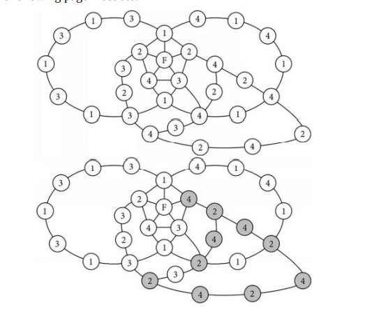
The previous diagrams show that when the two color reversals are performed one at a time in the crossed-chain graph, the first color reversal may break the other chain, allowing the second color reversal to affect the colors of one of F’s neighbors. When we performed the $2-4$ reversal to change B from 2 to 4 , this broke the 1-4 chain. When we then performed the 2-3 reversal to change E from 3, this caused C to change from 3 to 2 . As a result, F remains connected to four different colors; this wasn’t reversed to three as expected.
Unfortunately, you can’t perform both reversals “at the same time” for the following reason. Let’s attempt to perform both reversals “at the same time.” In this crossed-chain diagram, when we swap 2 and 4 on B’s side of the 1-3 chain, one of the 4’s in the 1-4 chain may change into a 2, and when we swap 2 and 3 on E’s side of the 1-4 chain, one of the 3’s in the 1-3 chain may change into a 2 . This is shown in the following figure: one 2 in each chain is shaded gray. Recall that these figures are incomplete; they focus on one vertex (F), its neighbors (A thru E), and Kempe chains. Other vertices and edges are not shown.

Note how one of the 3’s changed into 2 on the left. This can happen when we reverse $\mathrm{C}$ and $\mathrm{E}$ (which were originally 3 and 2 ) on E’s side of the 1-4 chain. Note also how one of the 4’s changed into 2 on the right. This can happen when we reverse B and D (which were originally 2 and 4) outside of the 1-3 chain. Now we see where a problem can occur when attempting to swap the colors of two chains at the same time. If these two 2’s happen to be connected by an edge like the dashed edge shown above, if we perform the double reversal at the same time, this causes two vertices of the same color to share an edge, which isn’t allowed. We’ll revisit Kempe’s strategy for coloring a vertex with degree five in Chapter $25 .$

图论代考

数学代写|图论作业代写Graph Theory代考|The shading of one section of the B-R

由于 Kempe 链的每个部分都与同一颜色对的其他部分隔离，因此 Kempe 链的任何部分的颜色可以颠倒，但仍满足四色定理。这是一个重要且有用的概念。

上面 BR 链的一个部分的阴影说明了任何 Kempe 链的任何部分的颜色如何可以反转。请注意，我们反转了 BR 链的一个部分的颜色，但没有反转中心部分的颜色。同一条链的每个部分的颜色可以独立于该链的其他部分反转。

为什么 PG 有 Kempe 链？很容易理解为什么 MPG 有 Kempe 链。（由于 PG 是通过从 MPG 中去除边缘而形成的，并且由于适用于 MPG 的着色也适用于 PG，因此 PG 也具有 Kempe 链。）

• MPG 是三角测量的。它由具有三个边和三个顶点的面组成。
• 每个面的三个顶点必须是三种不同的颜色。
• 每条边由两个相邻的三角形共享，形成一个四边形。
• 每个四边形将有 3 或 4 种不同的颜色。如果与共享边相对的两个顶点恰好是相同的颜色，则它有 3 种颜色。
• 对于每个四边形，四个顶点中的至少 1 个顶点和最多 3 个顶点具有任何颜色对的颜色。例如，具有 R、G、B 和G有 1 个顶点R−是和3个顶点乙−G，或者您可以将其视为 1 个顶点乙−是和3个顶点G−R，或者您可以将其视为 BR 的 2 个顶点和 GY 的 2 个顶点。在后一种情况下，2G’ 不是同一链的连续颜色。
• 当您将更多三角形组合在一起（四边形仅组合两个）并考虑可能的颜色时，您将看到 Kempe 的部分

链子出现。我们将在 Chápter 中看到这些 Kémpé chảins 是如何出现的21.
也很容易看出一对颜色（如 RY）将如何与其对应颜色（BG）相邻：

• 画一张R顶点和一个是由边连接的顶点。
• 如果一个新顶点连接到这些顶点中的每一个，它必须是乙或者G.
• 如果一个新顶点连接到 R 而不是是，可能是是,乙， 或者G.
• 如果一个新的顶点连接到是但不是R，可能是R,乙， 或者G.
• RY 链要么继续增长，要么被 B 包围，G.
• 如果你关注 B 和 G，你会为它的链条得出类似的结论。
• 如果一条链条完全被其对应物包围，则链条的新部分可能会出现在其对应物的另一侧。
  Kempe 证明了所有具有四阶的顶点（那些恰好连接到其他四个顶点的顶点）都是四色的 [Ref. 2]。例如，考虑下面的中心顶点。

数学代写|图论作业代写Graph Theory代考|In the previous figure

在上图中，顶点和是四度，因为它连接到其他四个顶点。Kempe 表明顶点 A、B、C 和 D 不能被强制为四种不同的颜色，这样顶点 E 总是可以被着色而不会违反四色定理，无论 MPG 的其余部分看起来如何上一页显示的部分。

• A 和 C 或者是 AC Kempe 链的同一部分的一部分，或者它们各自位于 AC Kempe 链的不同部分。（如果一种和C例如，是红色和黄色的，则 AC 链是红黄色链。） – 如果一种和C每个位于 AC Kempe 链的不同部分，其中一个部分的颜色可以反转，这有效地重新着色 C 以匹配 A 的颜色。如果 A 和 C 是 AC Kempe 链的同一部分的一部分，则 B 和 D每个都必须位于 BD Kempe 链的不同部分，因为 AC Kempe 链将阻止任何 BD Kempe 链从 B 到达 D。（如果乙和D是蓝色和绿色，例如，那么一种BD Kempe 链是蓝绿色链。）在这种情况下，由于 B 和 D 分别位于 BD Kempe 链的不同部分，因此 BD Kempe 链的其中一个部分的颜色可以反转，这有效地重新着色 D 以匹配 B颜色。– 因此，可以使 C 与 A 具有相同的颜色或使 D 具有与 A 相同的颜色乙通过反转 Kempe 链的分离部分。

上面的图表是不完整的。这些图只显示了一个四阶顶点（顶点 E）、它的最近邻居（A、B、C 和 D），以及 AC Kempe 链的片段。整个图还将包含几个其他顶点（特别是与 B 或 D 相同的颜色）和足够多的边以成为 MPG。左图有 A 连接到C在 AC Kempe 链的单个部分中（意味着该链的顶点颜色与 A 和 C 相同）。左图显示此 AC Kempe 链阻止 B 连接到DBD Kempe 链条的一个部分。中间的数字在 AC Kempe 链的不同部分有 A 和 C。在这种情况下，B 可以通过 BD Kempe 链的单个部分连接到 D。但是，由于四阶顶点的 A 和 C 位于不同的部分，因此可以反转 C 链的颜色，以便在四阶顶点中，C 有效地重新着色以匹配 A 的颜色，如右图所示. 类似地，可以在左图中反转 D 的部分，以便有效地重新着色 D 以匹配 B 的颜色。

Kempe 还试图证明五阶顶点是可四色的，以证明四色定理 [Ref. 2]，但 Heawood 在 1890 年证明他关于五次顶点的论点是不充分的 [Ref. 3]。让我们探讨一下如果我们尝试将我们对度数为四的顶点的推理应用于度数为五的顶点会发生什么。

数学代写|图论作业代写Graph Theory代考|The previous diagrams

前面的图表显示，当在交叉链图中一次执行两种颜色反转时，第一次颜色反转可能会破坏另一个链，从而允许第二次颜色反转影响 F 的一个邻居的颜色。当我们执行2−4反转将 B 从 2 更改为 4 ，这打破了 1-4 链。然后，当我们执行 2-3 反转以将 E 从 3 更改时，这导致 C 从 3 更改为 2 。结果，F 仍然连接到四种不同的颜色；这并没有像预期的那样反转为三个。
不幸的是，由于以下原因，您不能“同时”执行两个冲销。让我们尝试“同时”执行两个反转。在这个交叉链图中，当我们在 1-3 链的 B 侧交换 2 和 4 时，1-4 链中的一个 4 可能会变成 2，当我们在 E 侧交换 2 和 3 时1-4 链，1-3 链中的 3 之一可能会变为 2 。如下图所示：每条链中的一个 2 为灰色阴影。回想一下，这些数字是不完整的；他们专注于一个顶点 (F)、它的邻居 (A 到 E) 和 Kempe 链。其他顶点和边未显示。

请注意左侧的 3 之一如何变为 2。当我们反转时会发生这种情况C和和（最初是 3 和 2 ）在 1-4 链的 E 侧。还要注意 4 个中的一个如何在右侧变为 2。当我们在 1-3 链之外反转 B 和 D（最初是 2 和 4）时，就会发生这种情况。现在我们看到了尝试同时交换两条链的颜色时会出现问题的地方。如果这两个 2 恰好通过上图虚线这样的边连接起来，如果我们同时进行双重反转，就会导致两个相同颜色的顶点共享一条边，这是不允许的。我们将在第 1 章重新讨论 Kempe 为五阶顶点着色的策略25.

统计代写请认准statistics-lab™. statistics-lab™为您的留学生涯保驾护航。

金融工程代写

金融工程是使用数学技术来解决金融问题。金融工程使用计算机科学、统计学、经济学和应用数学领域的工具和知识来解决当前的金融问题，以及设计新的和创新的金融产品。

非参数统计代写

非参数统计指的是一种统计方法，其中不假设数据来自于由少数参数决定的规定模型；这种模型的例子包括正态分布模型和线性回归模型。

广义线性模型代考

广义线性模型（GLM）归属统计学领域，是一种应用灵活的线性回归模型。该模型允许因变量的偏差分布有除了正态分布之外的其它分布。

术语 广义线性模型（GLM）通常是指给定连续和/或分类预测因素的连续响应变量的常规线性回归模型。它包括多元线性回归，以及方差分析和方差分析（仅含固定效应）。

有限元方法代写

有限元方法（FEM）是一种流行的方法，用于数值解决工程和数学建模中出现的微分方程。典型的问题领域包括结构分析、传热、流体流动、质量运输和电磁势等传统领域。

有限元是一种通用的数值方法，用于解决两个或三个空间变量的偏微分方程（即一些边界值问题）。为了解决一个问题，有限元将一个大系统细分为更小、更简单的部分，称为有限元。这是通过在空间维度上的特定空间离散化来实现的，它是通过构建对象的网格来实现的：用于求解的数值域，它有有限数量的点。边界值问题的有限元方法表述最终导致一个代数方程组。该方法在域上对未知函数进行逼近。[1] 然后将模拟这些有限元的简单方程组合成一个更大的方程系统，以模拟整个问题。然后，有限元通过变化微积分使相关的误差函数最小化来逼近一个解决方案。

tatistics-lab作为专业的留学生服务机构，多年来已为美国、英国、加拿大、澳洲等留学热门地的学生提供专业的学术服务，包括但不限于Essay代写，Assignment代写，Dissertation代写，Report代写，小组作业代写，Proposal代写，Paper代写，Presentation代写，计算机作业代写，论文修改和润色，网课代做，exam代考等等。写作范围涵盖高中，本科，研究生等海外留学全阶段，辐射金融，经济学，会计学，审计学，管理学等全球99%专业科目。写作团队既有专业英语母语作者，也有海外名校硕博留学生，每位写作老师都拥有过硬的语言能力，专业的学科背景和学术写作经验。我们承诺100%原创，100%专业，100%准时，100%满意。

随机分析代写

随机微积分是数学的一个分支，对随机过程进行操作。它允许为随机过程的积分定义一个关于随机过程的一致的积分理论。这个领域是由日本数学家伊藤清在第二次世界大战期间创建并开始的。

时间序列分析代写

随机过程，是依赖于参数的一组随机变量的全体，参数通常是时间。 随机变量是随机现象的数量表现，其时间序列是一组按照时间发生先后顺序进行排列的数据点序列。通常一组时间序列的时间间隔为一恒定值（如1秒，5分钟，12小时，7天，1年），因此时间序列可以作为离散时间数据进行分析处理。研究时间序列数据的意义在于现实中，往往需要研究某个事物其随时间发展变化的规律。这就需要通过研究该事物过去发展的历史记录，以得到其自身发展的规律。

回归分析代写

多元回归分析渐进（Multiple Regression Analysis Asymptotics）属于计量经济学领域，主要是一种数学上的统计分析方法，可以分析复杂情况下各影响因素的数学关系，在自然科学、社会和经济学等多个领域内应用广泛。

MATLAB代写

MATLAB 是一种用于技术计算的高性能语言。它将计算、可视化和编程集成在一个易于使用的环境中，其中问题和解决方案以熟悉的数学符号表示。典型用途包括：数学和计算算法开发建模、仿真和原型制作数据分析、探索和可视化科学和工程图形应用程序开发，包括图形用户界面构建MATLAB 是一个交互式系统，其基本数据元素是一个不需要维度的数组。这使您可以解决许多技术计算问题，尤其是那些具有矩阵和向量公式的问题，而只需用 C 或 Fortran 等标量非交互式语言编写程序所需的时间的一小部分。MATLAB 名称代表矩阵实验室。MATLAB 最初的编写目的是提供对由 LINPACK 和 EISPACK 项目开发的矩阵软件的轻松访问，这两个项目共同代表了矩阵计算软件的最新技术。MATLAB 经过多年的发展，得到了许多用户的投入。在大学环境中，它是数学、工程和科学入门和高级课程的标准教学工具。在工业领域，MATLAB 是高效研究、开发和分析的首选工具。MATLAB 具有一系列称为工具箱的特定于应用程序的解决方案。对于大多数 MATLAB 用户来说非常重要，工具箱允许您学习和应用专业技术。工具箱是 MATLAB 函数（M 文件）的综合集合，可扩展 MATLAB 环境以解决特定类别的问题。可用工具箱的领域包括信号处理、控制系统、神经网络、模糊逻辑、小波、仿真等。

R语言代写	问卷设计与分析代写
PYTHON代写	回归分析与线性模型代写
MATLAB代写	方差分析与试验设计代写
STATA代写	机器学习/统计学习代写
SPSS代写	计量经济学代写
EVIEWS代写	时间序列分析代写
EXCEL代写	深度学习代写
SQL代写	各种数据建模与可视化代写

如果你也在 怎样代写数据科学、大数据和数据多样性Data Science, Big Data and Data Variety这个学科遇到相关的难题，请随时右上角联系我们的24/7代写客服。

数据科学是一个领域。大数据是一种收集、维护和处理巨大信息的技术。它是关于在各种操作中收集、处理、分析和利用数据。它更具有概念性。

statistics-lab™ 为您的留学生涯保驾护航 在代写数据科学、大数据和数据多样性Data Science, Big Data and Data Variety方面已经树立了自己的口碑, 保证靠谱, 高质且原创的统计Statistics代写服务。我们的专家在代写数据科学、大数据和数据多样性Data Science, Big Data and Data Variety代写方面经验极为丰富，各种代写数据科学、大数据和数据多样性Data Science, Big Data and Data Variety相关的作业也就用不着说。

我们提供的数据科学、大数据和数据多样性Data Science, Big Data and Data Variety及其相关学科的代写，服务范围广, 其中包括但不限于:

• Statistical Inference 统计推断
• Statistical Computing 统计计算
• Advanced Probability Theory 高等概率论
• Advanced Mathematical Statistics 高等数理统计学
• (Generalized) Linear Models 广义线性模型
• Statistical Machine Learning 统计机器学习
• Longitudinal Data Analysis 纵向数据分析
• Foundations of Data Science 数据科学基础

统计代写|数据科学、大数据和数据多样性代写Data Science, Big Data and Data Variety代考|Sample Frame Construction

The applications discussed in Section $1.3 .1$ have assumed that a population or frame already exists and have focused on leveraging known information about these units to create sample partitions or subsets using unsupervised MLMs. In some situations, however, the frames may overcover the target population and may require modification prior to segmentation to create sampling units that have a higher incidence for the target population. In yet other situations, no known frames or systematic collection of population units are available. To this end, a growing body of literature is focused on applying MLMs to create sampling frames or revise existing frames to improve coverage for the intended target population. Some of these applications use existing frame data, auxiliary data, and survey data to create models predicting whether or not population units in an existing frame belong to the target population while other applications use Big Data sources, such as satellite images, to create models that will identify locations of sampling units.
Garber (2009) used classification trees to predict eligibility of units included in a master mailing list for a survey targeting farms. Reductions in data collection inefficiencies due to overcoverage resulted from removing those units with low likelihood of eligibility. Bosch et al. (2018) discuss how they added web address information to a business register composed of a list of enterprises using a focused web scraping approach. Because the crawler might have misidentified the uniform record locator (URL), the team used MLMs to predict whether the URL was appropriate for each enterprise in the database. In this application, MLMs were not applied directly to identify population units or to segment them, but rather as part of the process for editing information on the frame obtained via web scraping methods. Chew et al. (2018) combine the approaches of frame refinement with frame creation by applying a two-category classification task to predict whether a satellite image scene is residential or nonresidential within a gridded population sampling framework.

Gridded samples use a geographic information system to partition areas of interest into logistically manageable grid cells for sampling (Thomson et al. 2017; Amer 2015). These designs typically involve several stages with one of the key stages selecting a series of primary grid units (PGUs) followed by a subselection of many secondary grid units (SGUs) within the PGUs. In many applications of this approach in developing countries, these SGUs are sparsely populated and consequently may have no eligible household units within them. To improve sampling efficiency, a layer of coding is often deployed within the selected PGUs to eliminate SGUs that contain no eligible population units prior to the phase of sampling that selects a subset of the SGUs.

统计代写|数据科学、大数据和数据多样性代写Data Science, Big Data and Data Variety代考|Considerations About Algorithmic Optimization

The results deemed optimal for grouping population units into groups based on an MLM may not be optimal for sampling or data collection. For example, some results from unsupervised learning models may produce groups with a single or too few population units to support the sampling design or estimation of sampling variance. Generally, for stratification, one wants a sample of at least two population units selected per group and in some cases, larger samples may be needed for other analytic objectives including comparisons across groups. In these cases, we need to ensure that the final segmentation has sufficient numbers of population units per unit. As Burgette et al. (2019, p. 6) point out “we are less concerned with model fit and more concerned with the sample characteristics that result from using the clusters [segments] as sample strata.”
The MLMs are using an objective for optimization that is related to what researchers desire – a natural grouping of population units into segments. However, to be useful for sampling, these segments may need to have a minimum size or the number of such segments may need to be constrained to meet sampling field operations requirements or data collection cost constraints, none of which are considered in the algorithms. That is, the requirements of sample designs and survey operations are not seen by current clustering algorithms during their processing of available data to create potential sampling strata or primary sampling unit groupings. As a result, the results from the MLM serve as the basis or first step that is then refined to meet additional sampling requirements or data collection constraints.

数据科学、大数据和数据多样性代考

统计代写|数据科学、大数据和数据多样性代写Data Science, Big Data and Data Variety代考|Sample Frame Construction

部分讨论的应用1.3.1假设人口或框架已经存在，并专注于利用有关这些单位的已知信息来使用无监督 MLM 创建样本分区或子集。然而，在某些情况下，框架可能会覆盖目标人群，并且可能需要在分割之前进行修改以创建对目标人群具有更高发生率的采样单元。在其他情况下，没有已知的框架或人口单位的系统集合可用。为此，越来越多的文献集中在应用 MLM 来创建抽样框架或修改现有框架以提高对预期目标人群的覆盖率。其中一些应用程序使用现有的帧数据、辅助数据、
Garber (2009) 使用分类树来预测包含在主邮件列表中的单位的资格，以进行针对农场的调查。由于过度覆盖导致数据收集效率低下的减少是由于移除了那些合格可能性较低的单位。博世等人。（2018 年）讨论他们如何使用集中的网络抓取方法将网址信息添加到由企业列表组成的企业注册中。由于爬虫可能错误地识别了统一记录定位器 (URL)，因此团队使用 MLM 来预测 URL 是否适合数据库中的每个企业。在此应用中，MLM 并未直接应用于识别人口单位或对其进行分割，而是作为编辑通过网络抓取方法获得的框架信息的过程的一部分。周等人。

网格化样本使用地理信息系统将感兴趣的区域划分为逻辑上可管理的网格单元以进行采样（Thomson 等人 2017；Amer 2015）。这些设计通常涉及多个阶段，其中一个关键阶段选择一系列主要电网单元 (PGU)，然后是 PGU 内的许多次要电网单元 (SGU) 的子选择。这种方法在发展中国家的许多应用中，这些 SGU 人口稀少，因此可能没有符合条件的住户单元。为了提高抽样效率，通常在选定的 PGU 中部署一层编码，以在选择 SGU 子集的抽样阶段之前消除不包含符合条件的人口单位的 SGU。

统计代写|数据科学、大数据和数据多样性代写Data Science, Big Data and Data Variety代考|Considerations About Algorithmic Optimization

基于 MLM 将人口单位分组为最佳的结果可能不是采样或数据收集的最佳结果。例如，来自无监督学习模型的一些结果可能会产生具有单个或太少人口单位的群体，以支持抽样设计或抽样方差的估计。一般来说，对于分层，人们希望每组至少选择两个人口单位的样本，在某些情况下，可能需要更大的样本用于其他分析目标，包括跨组比较。在这些情况下，我们需要确保最终的分割具有足够数量的每个单位的人口单位。作为 Burgette 等人。（2019 年，第 6 页）指出“我们不太关心模型拟合，而更关心使用集群 [segments] 作为样本层所产生的样本特征。”
传销使用与研究人员期望相关的优化目标 – 将人口单位自然分组为段。然而，为了对抽样有用，这些段可能需要具有最小大小，或者可能需要限制这些段的数量以满足抽样现场操作要求或数据收集成本限制，算法中没有考虑到这些。也就是说，当前的聚类算法在处理可用数据以创建潜在的抽样层或初级抽样单位分组时，没有看到样本设计和调查操作的要求。因此，来自 MLM 的结果可作为基础或第一步，然后对其进行细化以满足额外的抽样要求或数据收集限制。

统计代写请认准statistics-lab™. statistics-lab™为您的留学生涯保驾护航。

金融工程代写

金融工程是使用数学技术来解决金融问题。金融工程使用计算机科学、统计学、经济学和应用数学领域的工具和知识来解决当前的金融问题，以及设计新的和创新的金融产品。

非参数统计代写

非参数统计指的是一种统计方法，其中不假设数据来自于由少数参数决定的规定模型；这种模型的例子包括正态分布模型和线性回归模型。



广义线性模型代考

广义线性模型（GLM）归属统计学领域，是一种应用灵活的线性回归模型。该模型允许因变量的偏差分布有除了正态分布之外的其它分布。



术语 广义线性模型（GLM）通常是指给定连续和/或分类预测因素的连续响应变量的常规线性回归模型。它包括多元线性回归，以及方差分析和方差分析（仅含固定效应）。



有限元方法代写

有限元方法（FEM）是一种流行的方法，用于数值解决工程和数学建模中出现的微分方程。典型的问题领域包括结构分析、传热、流体流动、质量运输和电磁势等传统领域。

有限元是一种通用的数值方法，用于解决两个或三个空间变量的偏微分方程（即一些边界值问题）。为了解决一个问题，有限元将一个大系统细分为更小、更简单的部分，称为有限元。这是通过在空间维度上的特定空间离散化来实现的，它是通过构建对象的网格来实现的：用于求解的数值域，它有有限数量的点。边界值问题的有限元方法表述最终导致一个代数方程组。该方法在域上对未知函数进行逼近。[1] 然后将模拟这些有限元的简单方程组合成一个更大的方程系统，以模拟整个问题。然后，有限元通过变化微积分使相关的误差函数最小化来逼近一个解决方案。

tatistics-lab作为专业的留学生服务机构，多年来已为美国、英国、加拿大、澳洲等留学热门地的学生提供专业的学术服务，包括但不限于Essay代写，Assignment代写，Dissertation代写，Report代写，小组作业代写，Proposal代写，Paper代写，Presentation代写，计算机作业代写，论文修改和润色，网课代做，exam代考等等。写作范围涵盖高中，本科，研究生等海外留学全阶段，辐射金融，经济学，会计学，审计学，管理学等全球99%专业科目。写作团队既有专业英语母语作者，也有海外名校硕博留学生，每位写作老师都拥有过硬的语言能力，专业的学科背景和学术写作经验。我们承诺100%原创，100%专业，100%准时，100%满意。

随机分析代写

随机微积分是数学的一个分支，对随机过程进行操作。它允许为随机过程的积分定义一个关于随机过程的一致的积分理论。这个领域是由日本数学家伊藤清在第二次世界大战期间创建并开始的。

时间序列分析代写

随机过程，是依赖于参数的一组随机变量的全体，参数通常是时间。 随机变量是随机现象的数量表现，其时间序列是一组按照时间发生先后顺序进行排列的数据点序列。通常一组时间序列的时间间隔为一恒定值（如1秒，5分钟，12小时，7天，1年），因此时间序列可以作为离散时间数据进行分析处理。研究时间序列数据的意义在于现实中，往往需要研究某个事物其随时间发展变化的规律。这就需要通过研究该事物过去发展的历史记录，以得到其自身发展的规律。



回归分析代写

多元回归分析渐进（Multiple Regression Analysis Asymptotics）属于计量经济学领域，主要是一种数学上的统计分析方法，可以分析复杂情况下各影响因素的数学关系，在自然科学、社会和经济学等多个领域内应用广泛。

MATLAB代写

MATLAB 是一种用于技术计算的高性能语言。它将计算、可视化和编程集成在一个易于使用的环境中，其中问题和解决方案以熟悉的数学符号表示。典型用途包括：数学和计算算法开发建模、仿真和原型制作数据分析、探索和可视化科学和工程图形应用程序开发，包括图形用户界面构建MATLAB 是一个交互式系统，其基本数据元素是一个不需要维度的数组。这使您可以解决许多技术计算问题，尤其是那些具有矩阵和向量公式的问题，而只需用 C 或 Fortran 等标量非交互式语言编写程序所需的时间的一小部分。MATLAB 名称代表矩阵实验室。MATLAB 最初的编写目的是提供对由 LINPACK 和 EISPACK 项目开发的矩阵软件的轻松访问，这两个项目共同代表了矩阵计算软件的最新技术。MATLAB 经过多年的发展，得到了许多用户的投入。在大学环境中，它是数学、工程和科学入门和高级课程的标准教学工具。在工业领域，MATLAB 是高效研究、开发和分析的首选工具。MATLAB 具有一系列称为工具箱的特定于应用程序的解决方案。对于大多数 MATLAB 用户来说非常重要，工具箱允许您学习和应用专业技术。工具箱是 MATLAB 函数（M 文件）的综合集合，可扩展 MATLAB 环境以解决特定类别的问题。可用工具箱的领域包括信号处理、控制系统、神经网络、模糊逻辑、小波、仿真等。



R语言代写	问卷设计与分析代写
PYTHON代写	回归分析与线性模型代写
MATLAB代写	方差分析与试验设计代写
STATA代写	机器学习/统计学习代写
SPSS代写	计量经济学代写
EVIEWS代写	时间序列分析代写
EXCEL代写	深度学习代写
SQL代写	各种数据建模与可视化代写

The graphs above are incomplete. These figures only show a vertex with degree four (vertex E), its nearest neighbors (A, B, C, and D), and segments of A-C Kempe chains. The entire graphs would also contain several other vertices (especially, more colored the same as B or D) and enough edges to be MPG’s. The left figure has A connected to $C$ in a single section of an A-C Kempe chain (meaning that the vertices of this chain are colored the same as A and C). The left figure shows that this A-C Kempe chain prevents B from connecting to $\mathrm{D}$ with a single section of a B-D Kempe chain. The middle figure has A and C in separate sections of A-C Kempe chains. In this case, B could connect to D with a single section of a B-D Kempe chain. However, since the A and C of the vertex with degree four lie on separate sections, the color of C’s chain can be reversed so that in the vertex with degree four, C is effectively recolored to match A’s color, as shown in the right figure. Similarly, D’s section could be reversed in the left figure so that D is effectively recolored to match B’s color.

Kempe also attempted to demonstrate that vertices with degree five are fourcolorable in his attempt to prove the four-color theorem [Ref. 2], but his argument for vertices with degree five was shown by Heawood in 1890 to be insufficient [Ref. 3]. Let’s explore what happens if we attempt to apply our reasoning for vertices with degree four to a vertex with degree five.

数学代写|图论作业代写Graph Theory代考|The previous diagrams

The previous diagrams show that when the two color reversals are performed one at a time in the crossed-chain graph, the first color reversal may break the other chain, allowing the second color reversal to affect the colors of one of F’s neighbors. When we performed the $2-4$ reversal to change B from 2 to 4 , this broke the 1-4 chain. When we then performed the 2-3 reversal to change E from 3, this caused C to change from 3 to 2 . As a result, F remains connected to four different colors; this wasn’t reversed to three as expected.
Unfortunately, you can’t perform both reversals “at the same time” for the following reason. Let’s attempt to perform both reversals “at the same time.” In this crossed-chain diagram, when we swap 2 and 4 on B’s side of the 1-3 chain, one of the 4’s in the 1-4 chain may change into a 2, and when we swap 2 and 3 on E’s side of the 1-4 chain, one of the 3’s in the 1-3 chain may change into a 2 . This is shown in the following figure: one 2 in each chain is shaded gray. Recall that these figures are incomplete; they focus on one vertex (F), its neighbors (A thru E), and Kempe chains. Other vertices and edges are not shown.

Note how one of the 3’s changed into 2 on the left. This can happen when we reverse $\mathrm{C}$ and $\mathrm{E}$ (which were originally 3 and 2 ) on E’s side of the 1-4 chain. Note also how one of the 4’s changed into 2 on the right. This can happen when we reverse B and D (which were originally 2 and 4) outside of the 1-3 chain. Now we see where a problem can occur when attempting to swap the colors of two chains at the same time. If these two 2’s happen to be connected by an edge like the dashed edge shown above, if we perform the double reversal at the same time, this causes two vertices of the same color to share an edge, which isn’t allowed. We’ll revisit Kempe’s strategy for coloring a vertex with degree five in Chapter $25 .$

图论代考

数学代写|图论作业代写Graph Theory代考|The shading of one section of the B-R

由于 Kempe 链的每个部分都与同一颜色对的其他部分隔离，因此 Kempe 链的任何部分的颜色可以颠倒，但仍满足四色定理。这是一个重要且有用的概念。

上面 BR 链的一个部分的阴影说明了任何 Kempe 链的任何部分的颜色如何可以反转。请注意，我们反转了 BR 链的一个部分的颜色，但没有反转中心部分的颜色。同一条链的每个部分的颜色可以独立于该链的其他部分反转。

为什么 PG 有 Kempe 链？很容易理解为什么 MPG 有 Kempe 链。（由于 PG 是通过从 MPG 中去除边缘而形成的，并且由于适用于 MPG 的着色也适用于 PG，因此 PG 也具有 Kempe 链。）

• MPG 是三角测量的。它由具有三个边和三个顶点的面组成。
• 每个面的三个顶点必须是三种不同的颜色。
• 每条边由两个相邻的三角形共享，形成一个四边形。
• 每个四边形将有 3 或 4 种不同的颜色。如果与共享边相对的两个顶点恰好是相同的颜色，则它有 3 种颜色。
• 对于每个四边形，四个顶点中的至少 1 个顶点和最多 3 个顶点具有任何颜色对的颜色。例如，具有 R、G、B 和G有 1 个顶点R−是和3个顶点乙−G，或者您可以将其视为 1 个顶点乙−是和3个顶点G−R，或者您可以将其视为 BR 的 2 个顶点和 GY 的 2 个顶点。在后一种情况下，2G’ 不是同一链的连续颜色。
• 当您将更多三角形组合在一起（四边形仅组合两个）并考虑可能的颜色时，您将看到 Kempe 的部分

链子出现。我们将在 Chápter 中看到这些 Kémpé chảins 是如何出现的21.
也很容易看出一对颜色（如 RY）将如何与其对应颜色（BG）相邻：

• 画一张R顶点和一个是由边连接的顶点。
• 如果一个新顶点连接到这些顶点中的每一个，它必须是乙或者G.
• 如果一个新顶点连接到 R 而不是是，可能是是,乙， 或者G.
• 如果一个新的顶点连接到是但不是R，可能是R,乙， 或者G.
• RY 链要么继续增长，要么被 B 包围，G.
• 如果你关注 B 和 G，你会为它的链条得出类似的结论。
• 如果一条链条完全被其对应物包围，则链条的新部分可能会出现在其对应物的另一侧。
  Kempe 证明了所有具有四阶的顶点（那些恰好连接到其他四个顶点的顶点）都是四色的 [Ref. 2]。例如，考虑下面的中心顶点。

数学代写|图论作业代写Graph Theory代考|In the previous figure

在上图中，顶点和是四度，因为它连接到其他四个顶点。Kempe 表明顶点 A、B、C 和 D 不能被强制为四种不同的颜色，这样顶点 E 总是可以被着色而不会违反四色定理，无论 MPG 的其余部分看起来如何上一页显示的部分。

• A 和 C 或者是 AC Kempe 链的同一部分的一部分，或者它们各自位于 AC Kempe 链的不同部分。（如果一种和C例如，是红色和黄色的，则 AC 链是红黄色链。） – 如果一种和C每个位于 AC Kempe 链的不同部分，其中一个部分的颜色可以反转，这有效地重新着色 C 以匹配 A 的颜色。如果 A 和 C 是 AC Kempe 链的同一部分的一部分，则 B 和 D每个都必须位于 BD Kempe 链的不同部分，因为 AC Kempe 链将阻止任何 BD Kempe 链从 B 到达 D。（如果乙和D是蓝色和绿色，例如，那么一种BD Kempe 链是蓝绿色链。）在这种情况下，由于 B 和 D 分别位于 BD Kempe 链的不同部分，因此 BD Kempe 链的其中一个部分的颜色可以反转，这有效地重新着色 D 以匹配 B颜色。– 因此，可以使 C 与 A 具有相同的颜色或使 D 具有与 A 相同的颜色乙通过反转 Kempe 链的分离部分。

上面的图表是不完整的。这些图只显示了一个四阶顶点（顶点 E）、它的最近邻居（A、B、C 和 D），以及 AC Kempe 链的片段。整个图还将包含几个其他顶点（特别是与 B 或 D 相同的颜色）和足够多的边以成为 MPG。左图有 A 连接到C在 AC Kempe 链的单个部分中（意味着该链的顶点颜色与 A 和 C 相同）。左图显示此 AC Kempe 链阻止 B 连接到DBD Kempe 链条的一个部分。中间的数字在 AC Kempe 链的不同部分有 A 和 C。在这种情况下，B 可以通过 BD Kempe 链的单个部分连接到 D。但是，由于四阶顶点的 A 和 C 位于不同的部分，因此可以反转 C 链的颜色，以便在四阶顶点中，C 有效地重新着色以匹配 A 的颜色，如右图所示. 类似地，可以在左图中反转 D 的部分，以便有效地重新着色 D 以匹配 B 的颜色。

Kempe 还试图证明五阶顶点是可四色的，以证明四色定理 [Ref. 2]，但 Heawood 在 1890 年证明他关于五次顶点的论点是不充分的 [Ref. 3]。让我们探讨一下如果我们尝试将我们对度数为四的顶点的推理应用于度数为五的顶点会发生什么。

数学代写|图论作业代写Graph Theory代考|The previous diagrams

前面的图表显示，当在交叉链图中一次执行两种颜色反转时，第一次颜色反转可能会破坏另一个链，从而允许第二次颜色反转影响 F 的一个邻居的颜色。当我们执行2−4反转将 B 从 2 更改为 4 ，这打破了 1-4 链。然后，当我们执行 2-3 反转以将 E 从 3 更改时，这导致 C 从 3 更改为 2 。结果，F 仍然连接到四种不同的颜色；这并没有像预期的那样反转为三个。
不幸的是，由于以下原因，您不能“同时”执行两个冲销。让我们尝试“同时”执行两个反转。在这个交叉链图中，当我们在 1-3 链的 B 侧交换 2 和 4 时，1-4 链中的一个 4 可能会变成 2，当我们在 E 侧交换 2 和 3 时1-4 链，1-3 链中的 3 之一可能会变为 2 。如下图所示：每条链中的一个 2 为灰色阴影。回想一下，这些数字是不完整的；他们专注于一个顶点 (F)、它的邻居 (A 到 E) 和 Kempe 链。其他顶点和边未显示。

请注意左侧的 3 之一如何变为 2。当我们反转时会发生这种情况C和和（最初是 3 和 2 ）在 1-4 链的 E 侧。还要注意 4 个中的一个如何在右侧变为 2。当我们在 1-3 链之外反转 B 和 D（最初是 2 和 4）时，就会发生这种情况。现在我们看到了尝试同时交换两条链的颜色时会出现问题的地方。如果这两个 2 恰好通过上图虚线这样的边连接起来，如果我们同时进行双重反转，就会导致两个相同颜色的顶点共享一条边，这是不允许的。我们将在第 1 章重新讨论 Kempe 为五阶顶点着色的策略25.

统计代写请认准statistics-lab™. statistics-lab™为您的留学生涯保驾护航。

金融工程代写

金融工程是使用数学技术来解决金融问题。金融工程使用计算机科学、统计学、经济学和应用数学领域的工具和知识来解决当前的金融问题，以及设计新的和创新的金融产品。

非参数统计代写

非参数统计指的是一种统计方法，其中不假设数据来自于由少数参数决定的规定模型；这种模型的例子包括正态分布模型和线性回归模型。

广义线性模型代考

广义线性模型（GLM）归属统计学领域，是一种应用灵活的线性回归模型。该模型允许因变量的偏差分布有除了正态分布之外的其它分布。

术语 广义线性模型（GLM）通常是指给定连续和/或分类预测因素的连续响应变量的常规线性回归模型。它包括多元线性回归，以及方差分析和方差分析（仅含固定效应）。

有限元方法代写

有限元方法（FEM）是一种流行的方法，用于数值解决工程和数学建模中出现的微分方程。典型的问题领域包括结构分析、传热、流体流动、质量运输和电磁势等传统领域。

有限元是一种通用的数值方法，用于解决两个或三个空间变量的偏微分方程（即一些边界值问题）。为了解决一个问题，有限元将一个大系统细分为更小、更简单的部分，称为有限元。这是通过在空间维度上的特定空间离散化来实现的，它是通过构建对象的网格来实现的：用于求解的数值域，它有有限数量的点。边界值问题的有限元方法表述最终导致一个代数方程组。该方法在域上对未知函数进行逼近。[1] 然后将模拟这些有限元的简单方程组合成一个更大的方程系统，以模拟整个问题。然后，有限元通过变化微积分使相关的误差函数最小化来逼近一个解决方案。

tatistics-lab作为专业的留学生服务机构，多年来已为美国、英国、加拿大、澳洲等留学热门地的学生提供专业的学术服务，包括但不限于Essay代写，Assignment代写，Dissertation代写，Report代写，小组作业代写，Proposal代写，Paper代写，Presentation代写，计算机作业代写，论文修改和润色，网课代做，exam代考等等。写作范围涵盖高中，本科，研究生等海外留学全阶段，辐射金融，经济学，会计学，审计学，管理学等全球99%专业科目。写作团队既有专业英语母语作者，也有海外名校硕博留学生，每位写作老师都拥有过硬的语言能力，专业的学科背景和学术写作经验。我们承诺100%原创，100%专业，100%准时，100%满意。

随机分析代写

随机微积分是数学的一个分支，对随机过程进行操作。它允许为随机过程的积分定义一个关于随机过程的一致的积分理论。这个领域是由日本数学家伊藤清在第二次世界大战期间创建并开始的。

时间序列分析代写

随机过程，是依赖于参数的一组随机变量的全体，参数通常是时间。 随机变量是随机现象的数量表现，其时间序列是一组按照时间发生先后顺序进行排列的数据点序列。通常一组时间序列的时间间隔为一恒定值（如1秒，5分钟，12小时，7天，1年），因此时间序列可以作为离散时间数据进行分析处理。研究时间序列数据的意义在于现实中，往往需要研究某个事物其随时间发展变化的规律。这就需要通过研究该事物过去发展的历史记录，以得到其自身发展的规律。

回归分析代写

多元回归分析渐进（Multiple Regression Analysis Asymptotics）属于计量经济学领域，主要是一种数学上的统计分析方法，可以分析复杂情况下各影响因素的数学关系，在自然科学、社会和经济学等多个领域内应用广泛。

MATLAB代写

MATLAB 是一种用于技术计算的高性能语言。它将计算、可视化和编程集成在一个易于使用的环境中，其中问题和解决方案以熟悉的数学符号表示。典型用途包括：数学和计算算法开发建模、仿真和原型制作数据分析、探索和可视化科学和工程图形应用程序开发，包括图形用户界面构建MATLAB 是一个交互式系统，其基本数据元素是一个不需要维度的数组。这使您可以解决许多技术计算问题，尤其是那些具有矩阵和向量公式的问题，而只需用 C 或 Fortran 等标量非交互式语言编写程序所需的时间的一小部分。MATLAB 名称代表矩阵实验室。MATLAB 最初的编写目的是提供对由 LINPACK 和 EISPACK 项目开发的矩阵软件的轻松访问，这两个项目共同代表了矩阵计算软件的最新技术。MATLAB 经过多年的发展，得到了许多用户的投入。在大学环境中，它是数学、工程和科学入门和高级课程的标准教学工具。在工业领域，MATLAB 是高效研究、开发和分析的首选工具。MATLAB 具有一系列称为工具箱的特定于应用程序的解决方案。对于大多数 MATLAB 用户来说非常重要，工具箱允许您学习和应用专业技术。工具箱是 MATLAB 函数（M 文件）的综合集合，可扩展 MATLAB 环境以解决特定类别的问题。可用工具箱的领域包括信号处理、控制系统、神经网络、模糊逻辑、小波、仿真等。

R语言代写	问卷设计与分析代写
PYTHON代写	回归分析与线性模型代写
MATLAB代写	方差分析与试验设计代写
STATA代写	机器学习/统计学习代写
SPSS代写	计量经济学代写
EVIEWS代写	时间序列分析代写
EXCEL代写	深度学习代写
SQL代写	各种数据建模与可视化代写

如果你也在 怎样代写数据科学、大数据和数据多样性Data Science, Big Data and Data Variety这个学科遇到相关的难题，请随时右上角联系我们的24/7代写客服。

数据科学是一个领域。大数据是一种收集、维护和处理巨大信息的技术。它是关于在各种操作中收集、处理、分析和利用数据。它更具有概念性。

statistics-lab™ 为您的留学生涯保驾护航 在代写数据科学、大数据和数据多样性Data Science, Big Data and Data Variety方面已经树立了自己的口碑, 保证靠谱, 高质且原创的统计Statistics代写服务。我们的专家在代写数据科学、大数据和数据多样性Data Science, Big Data and Data Variety代写方面经验极为丰富，各种代写数据科学、大数据和数据多样性Data Science, Big Data and Data Variety相关的作业也就用不着说。

我们提供的数据科学、大数据和数据多样性Data Science, Big Data and Data Variety及其相关学科的代写，服务范围广, 其中包括但不限于:

• Statistical Inference 统计推断
• Statistical Computing 统计计算
• Advanced Probability Theory 高等概率论
• Advanced Mathematical Statistics 高等数理统计学
• (Generalized) Linear Models 广义线性模型
• Statistical Machine Learning 统计机器学习
• Longitudinal Data Analysis 纵向数据分析
• Foundations of Data Science 数据科学基础

统计代写|数据科学、大数据和数据多样性代写Data Science, Big Data and Data Variety代考|Overview of Machine Learning Methods

MLMs are generally flexible, nonparametric methods for making predictions or classifications from data. These methods are typically described by the algorithm that details how the predictions are made using the raw data and can allow for a larger number of predictors, referred to as high-dimensional data. These methods can often automatically detect nonlinearities in the relationships between independent and dependent variables and can identify interactions automatically. Generally, MLMs can be divided into two broad categories: supervised and unsupervised machine learning techniques. The goal of supervised learning is to optimally predict a dependent variable (also referred to as output, target, class, or label), based on a range of independent variables (also referred to as inputs, features, or attributes). When a supervised method is applied to predict continuous outcomes, it is generally referred to as a regression problem and a classification problem when used to predict levels of a categorical variable. Ordinary least squares regression is a classic example of supervised machine learning. Such a technique relies on a single (continuous) dependent variable and seeks to determine the best linear fit between this outcome and multiple independent variables. MLMs can also be used to group cases based on a collection of variables known for all the cases. In these situations, there is no single outcome of interest and MLMs that are used in this context are referred to as unsupervised learners. One of the most common unsupervised methods with which social scientists and market researchers might have some familiarity is hierarchical cluster analysis (HCA) – also known as segmentation. In this case, the main interest is not on modeling an outcome based on multiple independent variables, as in regression, but rather on understanding if there are combinations of variables (e.g. demographics) that can segment or group sets of customers, respondents, or members of a group, class, or city. The final output of this approach is the actual grouping of the cases within a dataset – where the grouping is determined by the collection of variables available for the analysis.
Unlike many traditional modeling techniques such as ordinary least squares regression, MLMs require a specification of hyperparameters or tuning parameters before a final model and predictions can be obtained. These parameters are often estimated from the data prior to estimating the final model. It could be useful to think of these as settings or “knobs” on the “machine” prior to hitting the start button to generate the predictions. One of the simplest examples of a tuning parameter comes from $k$-means clustering. Prior to running a $k$-means clustering algorithm, the method needs to know how many clusters it should produce in the end (i.e. $K$ ). The main point is that these tuning parameters are needed before computing final models and predictions.

统计代写|数据科学、大数据和数据多样性代写Data Science, Big Data and Data Variety代考|Sample Design Creation

Many early applications of MLMs for sample design development focused on using these algorithms to create partitions of known population units into optimal groupings to facilitate stratified sampling or some other type of sampling designs. In particular, these approaches apply various types of unsupervised machine learning algorithms such as $k$-means clustering or Gaussian mixture models (GMMs) to an array of frame data and other auxiliary information to segment population units into groups for use as primary sampling units or strata for sampling designs. The population might also refer to a survey panel and auxiliary information might refer to typical frame-related variables as well as survey variables collected during prior phases. In either case, the goal of these approaches is to optimize segmentation of population units into groups that are efficient for sampling rather than on optimizing model fit. Evaluation of the final groupings obtained from the MLMs considers implications for both sampling errors and operational issues.

Although the literature illustrating applications of these types of unsupervised machine learning algorithms for developing sampling designs is small, it is growing. Burgette et al. (2019) compared three different unsupervised learning methods to create sampling strata to understand the range of care delivery structures and processes being deployed to influence the total costs of caring for patients over time. More specifically, their team compared $k$-means clustering to a mixture of normals (also referred to as GMMs) and mixture of regression models for clustering annual total cost of care statistics over a three-year period for some 40 physician organizations participating in the Integrated Healthcare Association’s value-based pay-for-performance program. Of primary interest was the total cost of care and its pattern over this period, so developing a design that groups physician organizations by total cost trajectories and magnitude was crucial. The cluster groupings from each of the three methods considered formed the basis of sampling strata. Burgette et al. (2019) evaluated the results from each method and decided on the results produced using the mixture of normals for their final sampling strata.
The work of Burgette and colleagues highlighted some key, important differences in the assumptions and mechanics of the three clustering methods. Most notably, the $k$-means clustering algorithm is concerned with differences about the cluster means and assumes that the within-cluster variances are equal, and the algorithm seeks to group units so as to minimize this within-cluster variance across the $k$-clusters. A common assumption in many models such as ANOVA is that the assumption of equal stratum variances may be too restrictive and not reasonable. The optimal number of clusters generated from the $k$-means algorithm taken as strata will be too heterogeneous relative to other stratifications that focus on grouping sampling units to reduce variation within each stratum without the restriction or assumption that this reduced variance is the same for every stratum. Burgette et al. (2019) note that the mixture of normal models does not have the assumption of equal variance within each of the clusters and allows this variance to vary within the resulting clusters. The mixture of normal models also allows researchers to incorporate a unit of size as an additional input into the modeling process separate from the variables upon which clustering is based.

数据科学、大数据和数据多样性代考

统计代写|数据科学、大数据和数据多样性代写Data Science, Big Data and Data Variety代考|Overview of Machine Learning Methods

传销通常是灵活的、非参数的方法，用于根据数据进行预测或分类。这些方法通常由算法描述，该算法详细说明了如何使用原始数据进行预测，并且可以允许更多的预测变量，称为高维数据。这些方法通常可以自动检测自变量和因变量之间关系中的非线性，并可以自动识别相互作用。一般来说，传销可以分为两大类：监督和非监督机器学习技术。监督学习的目标是根据一系列自变量（也称为输入、特征或属性）对因变量（也称为输出、目标、类别或标签）进行最佳预测。当使用监督方法来预测连续结果时，当用于预测分类变量的水平时，它通常被称为回归问题和分类问题。普通最小二乘回归是监督机器学习的一个经典例子。这种技术依赖于单个（连续）因变量，并试图确定该结果与多个自变量之间的最佳线性拟合。MLM 还可用于根据所有案例已知的变量集合对案例进行分组。在这些情况下，没有一个感兴趣的结果，在这种情况下使用的 MLM 被称为无监督学习器。社会科学家和市场研究人员可能熟悉的最常见的无监督方法之一是层次聚类分析 (HCA)，也称为分割。在这种情况下，主要兴趣不是基于多个自变量对结果进行建模，如回归，而是了解是否存在可以对客户、受访者或成员集进行细分或分组的变量组合（例如人口统计）一个群体、阶级或城市。这种方法的最终输出是数据集中案例的实际分组——其中分组由可用于分析的变量的集合确定。而是了解是否有变量组合（例如人口统计）可以细分或分组客户、受访者或组、类或城市的成员。这种方法的最终输出是数据集中案例的实际分组——其中分组由可用于分析的变量的集合确定。而是了解是否有变量组合（例如人口统计）可以细分或分组客户、受访者或组、类或城市的成员。这种方法的最终输出是数据集中案例的实际分组——其中分组由可用于分析的变量的集合确定。
与许多传统建模技术（例如普通最小二乘回归）不同，MLM 在获得最终模型和预测之前需要指定超参数或调整参数。这些参数通常是在估计最终模型之前从数据中估计的。在点击开始按钮生成预测之前，将这些视为“机器”上的设置或“旋钮”可能会很有用。调整参数的最简单示例之一来自ķ- 表示聚类。在运行之前ķ-means 聚类算法，该方法需要知道它最终应该产生多少个聚类（即ķ）。要点是在计算最终模型和预测之前需要这些调整参数。

统计代写|数据科学、大数据和数据多样性代写Data Science, Big Data and Data Variety代考|Sample Design Creation

MLM 在样本设计开发中的许多早期应用都集中在使用这些算法将已知人口单位划分为最佳分组，以促进分层抽样或其他一些类型的抽样设计。特别是，这些方法应用了各种类型的无监督机器学习算法，例如ķ- 将聚类或高斯混合模型 (GMM) 用于帧数据数组和其他辅助信息，以将人口单位划分为组，用作抽样设计的初级抽样单位或分层。人口也可能指调查小组，辅助信息可能指典型的框架相关变量以及在先前阶段收集的调查变量。在任何一种情况下，这些方法的目标都是优化将人口单位分割成对抽样有效的组，而不是优化模型拟合。对从 MLM 获得的最终分组的评估考虑了对抽样误差和操作问题的影响。

尽管说明这些类型的无监督机器学习算法在开发抽样设计中的应用的文献很少，但它正在增长。Burgette 等人。（2019 年）比较了三种不同的无监督学习方法来创建抽样层，以了解正在部署的护理提供结构和流程的范围，以影响随着时间的推移护理患者的总成本。更具体地说，他们的团队比较了ķ-意味着对参与综合医疗保健协会基于价值的薪酬的大约 40 家医生组织在三年期间对年度总护理成本统计数据进行聚类，以混合正常值（也称为 GMM）和回归模型的混合-绩效计划。主要关注的是这一时期的总护理成本及其模式，因此开发一种按总成本轨迹和规模对医生组织进行分组的设计至关重要。所考虑的三种方法中的每一种方法的聚类分组构成了抽样层的基础。Burgette 等人。（2019 年）评估了每种方法的结果，并决定使用混合法线作为最终抽样层产生的结果。
Burgette 及其同事的工作强调了三种聚类方法的假设和机制中的一些关键的重要差异。最值得注意的是，ķ-means 聚类算法关注关于聚类均值的差异，并假设聚类内方差相等，并且该算法寻求对单元进行分组以最小化整个聚类中的聚类内方差ķ-集群。许多模型（如 ANOVA）中的一个常见假设是等层方差的假设可能过于严格且不合理。生成的最佳聚类数ķ-均值算法相对于其他分层而言，作为分层将过于异质，这些分层侧重于对抽样单元进行分组以减少每个分层内的变化，而没有限制或假设这种减少的方差对于每个分层都是相同的。Burgette 等人。（2019）注意到，正常模型的混合没有假设每个集群内的方差相等，并允许这种方差在结果集群内变化。正常模型的混合还允许研究人员将一个大小单位作为附加输入纳入建模过程，与聚类所基于的变量分开。

统计代写请认准statistics-lab™. statistics-lab™为您的留学生涯保驾护航。

金融工程代写

金融工程是使用数学技术来解决金融问题。金融工程使用计算机科学、统计学、经济学和应用数学领域的工具和知识来解决当前的金融问题，以及设计新的和创新的金融产品。

非参数统计代写

非参数统计指的是一种统计方法，其中不假设数据来自于由少数参数决定的规定模型；这种模型的例子包括正态分布模型和线性回归模型。



广义线性模型代考

广义线性模型（GLM）归属统计学领域，是一种应用灵活的线性回归模型。该模型允许因变量的偏差分布有除了正态分布之外的其它分布。



术语 广义线性模型（GLM）通常是指给定连续和/或分类预测因素的连续响应变量的常规线性回归模型。它包括多元线性回归，以及方差分析和方差分析（仅含固定效应）。



有限元方法代写

有限元方法（FEM）是一种流行的方法，用于数值解决工程和数学建模中出现的微分方程。典型的问题领域包括结构分析、传热、流体流动、质量运输和电磁势等传统领域。

有限元是一种通用的数值方法，用于解决两个或三个空间变量的偏微分方程（即一些边界值问题）。为了解决一个问题，有限元将一个大系统细分为更小、更简单的部分，称为有限元。这是通过在空间维度上的特定空间离散化来实现的，它是通过构建对象的网格来实现的：用于求解的数值域，它有有限数量的点。边界值问题的有限元方法表述最终导致一个代数方程组。该方法在域上对未知函数进行逼近。[1] 然后将模拟这些有限元的简单方程组合成一个更大的方程系统，以模拟整个问题。然后，有限元通过变化微积分使相关的误差函数最小化来逼近一个解决方案。

tatistics-lab作为专业的留学生服务机构，多年来已为美国、英国、加拿大、澳洲等留学热门地的学生提供专业的学术服务，包括但不限于Essay代写，Assignment代写，Dissertation代写，Report代写，小组作业代写，Proposal代写，Paper代写，Presentation代写，计算机作业代写，论文修改和润色，网课代做，exam代考等等。写作范围涵盖高中，本科，研究生等海外留学全阶段，辐射金融，经济学，会计学，审计学，管理学等全球99%专业科目。写作团队既有专业英语母语作者，也有海外名校硕博留学生，每位写作老师都拥有过硬的语言能力，专业的学科背景和学术写作经验。我们承诺100%原创，100%专业，100%准时，100%满意。

随机分析代写

随机微积分是数学的一个分支，对随机过程进行操作。它允许为随机过程的积分定义一个关于随机过程的一致的积分理论。这个领域是由日本数学家伊藤清在第二次世界大战期间创建并开始的。

时间序列分析代写

随机过程，是依赖于参数的一组随机变量的全体，参数通常是时间。 随机变量是随机现象的数量表现，其时间序列是一组按照时间发生先后顺序进行排列的数据点序列。通常一组时间序列的时间间隔为一恒定值（如1秒，5分钟，12小时，7天，1年），因此时间序列可以作为离散时间数据进行分析处理。研究时间序列数据的意义在于现实中，往往需要研究某个事物其随时间发展变化的规律。这就需要通过研究该事物过去发展的历史记录，以得到其自身发展的规律。



回归分析代写

多元回归分析渐进（Multiple Regression Analysis Asymptotics）属于计量经济学领域，主要是一种数学上的统计分析方法，可以分析复杂情况下各影响因素的数学关系，在自然科学、社会和经济学等多个领域内应用广泛。

MATLAB代写

MATLAB 是一种用于技术计算的高性能语言。它将计算、可视化和编程集成在一个易于使用的环境中，其中问题和解决方案以熟悉的数学符号表示。典型用途包括：数学和计算算法开发建模、仿真和原型制作数据分析、探索和可视化科学和工程图形应用程序开发，包括图形用户界面构建MATLAB 是一个交互式系统，其基本数据元素是一个不需要维度的数组。这使您可以解决许多技术计算问题，尤其是那些具有矩阵和向量公式的问题，而只需用 C 或 Fortran 等标量非交互式语言编写程序所需的时间的一小部分。MATLAB 名称代表矩阵实验室。MATLAB 最初的编写目的是提供对由 LINPACK 和 EISPACK 项目开发的矩阵软件的轻松访问，这两个项目共同代表了矩阵计算软件的最新技术。MATLAB 经过多年的发展，得到了许多用户的投入。在大学环境中，它是数学、工程和科学入门和高级课程的标准教学工具。在工业领域，MATLAB 是高效研究、开发和分析的首选工具。MATLAB 具有一系列称为工具箱的特定于应用程序的解决方案。对于大多数 MATLAB 用户来说非常重要，工具箱允许您学习和应用专业技术。工具箱是 MATLAB 函数（M 文件）的综合集合，可扩展 MATLAB 环境以解决特定类别的问题。可用工具箱的领域包括信号处理、控制系统、神经网络、模糊逻辑、小波、仿真等。



R语言代写	问卷设计与分析代写
PYTHON代写	回归分析与线性模型代写
MATLAB代写	方差分析与试验设计代写
STATA代写	机器学习/统计学习代写
SPSS代写	计量经济学代写
EVIEWS代写	时间序列分析代写
EXCEL代写	深度学习代写
SQL代写	各种数据建模与可视化代写

The graphs above are incomplete. These figures only show a vertex with degree four (vertex E), its nearest neighbors (A, B, C, and D), and segments of A-C Kempe chains. The entire graphs would also contain several other vertices (especially, more colored the same as B or D) and enough edges to be MPG’s. The left figure has A connected to $C$ in a single section of an A-C Kempe chain (meaning that the vertices of this chain are colored the same as A and C). The left figure shows that this A-C Kempe chain prevents B from connecting to $\mathrm{D}$ with a single section of a B-D Kempe chain. The middle figure has A and C in separate sections of A-C Kempe chains. In this case, B could connect to D with a single section of a B-D Kempe chain. However, since the A and C of the vertex with degree four lie on separate sections, the color of C’s chain can be reversed so that in the vertex with degree four, C is effectively recolored to match A’s color, as shown in the right figure. Similarly, D’s section could be reversed in the left figure so that D is effectively recolored to match B’s color.

Kempe also attempted to demonstrate that vertices with degree five are fourcolorable in his attempt to prove the four-color theorem [Ref. 2], but his argument for vertices with degree five was shown by Heawood in 1890 to be insufficient [Ref. 3]. Let’s explore what happens if we attempt to apply our reasoning for vertices with degree four to a vertex with degree five.

数学代写|图论作业代写Graph Theory代考|The previous diagrams

The previous diagrams show that when the two color reversals are performed one at a time in the crossed-chain graph, the first color reversal may break the other chain, allowing the second color reversal to affect the colors of one of F’s neighbors. When we performed the $2-4$ reversal to change B from 2 to 4 , this broke the 1-4 chain. When we then performed the 2-3 reversal to change E from 3, this caused C to change from 3 to 2 . As a result, F remains connected to four different colors; this wasn’t reversed to three as expected.
Unfortunately, you can’t perform both reversals “at the same time” for the following reason. Let’s attempt to perform both reversals “at the same time.” In this crossed-chain diagram, when we swap 2 and 4 on B’s side of the 1-3 chain, one of the 4’s in the 1-4 chain may change into a 2, and when we swap 2 and 3 on E’s side of the 1-4 chain, one of the 3’s in the 1-3 chain may change into a 2 . This is shown in the following figure: one 2 in each chain is shaded gray. Recall that these figures are incomplete; they focus on one vertex (F), its neighbors (A thru E), and Kempe chains. Other vertices and edges are not shown.

Note how one of the 3’s changed into 2 on the left. This can happen when we reverse $\mathrm{C}$ and $\mathrm{E}$ (which were originally 3 and 2 ) on E’s side of the 1-4 chain. Note also how one of the 4’s changed into 2 on the right. This can happen when we reverse B and D (which were originally 2 and 4) outside of the 1-3 chain. Now we see where a problem can occur when attempting to swap the colors of two chains at the same time. If these two 2’s happen to be connected by an edge like the dashed edge shown above, if we perform the double reversal at the same time, this causes two vertices of the same color to share an edge, which isn’t allowed. We’ll revisit Kempe’s strategy for coloring a vertex with degree five in Chapter $25 .$

图论代考

数学代写|图论作业代写Graph Theory代考|The shading of one section of the B-R

由于 Kempe 链的每个部分都与同一颜色对的其他部分隔离，因此 Kempe 链的任何部分的颜色可以颠倒，但仍满足四色定理。这是一个重要且有用的概念。

上面 BR 链的一个部分的阴影说明了任何 Kempe 链的任何部分的颜色如何可以反转。请注意，我们反转了 BR 链的一个部分的颜色，但没有反转中心部分的颜色。同一条链的每个部分的颜色可以独立于该链的其他部分反转。

为什么 PG 有 Kempe 链？很容易理解为什么 MPG 有 Kempe 链。（由于 PG 是通过从 MPG 中去除边缘而形成的，并且由于适用于 MPG 的着色也适用于 PG，因此 PG 也具有 Kempe 链。）

• MPG 是三角测量的。它由具有三个边和三个顶点的面组成。
• 每个面的三个顶点必须是三种不同的颜色。
• 每条边由两个相邻的三角形共享，形成一个四边形。
• 每个四边形将有 3 或 4 种不同的颜色。如果与共享边相对的两个顶点恰好是相同的颜色，则它有 3 种颜色。
• 对于每个四边形，四个顶点中的至少 1 个顶点和最多 3 个顶点具有任何颜色对的颜色。例如，具有 R、G、B 和G有 1 个顶点R−是和3个顶点乙−G，或者您可以将其视为 1 个顶点乙−是和3个顶点G−R，或者您可以将其视为 BR 的 2 个顶点和 GY 的 2 个顶点。在后一种情况下，2G’ 不是同一链的连续颜色。
• 当您将更多三角形组合在一起（四边形仅组合两个）并考虑可能的颜色时，您将看到 Kempe 的部分

链子出现。我们将在 Chápter 中看到这些 Kémpé chảins 是如何出现的21.
也很容易看出一对颜色（如 RY）将如何与其对应颜色（BG）相邻：

• 画一张R顶点和一个是由边连接的顶点。
• 如果一个新顶点连接到这些顶点中的每一个，它必须是乙或者G.
• 如果一个新顶点连接到 R 而不是是，可能是是,乙， 或者G.
• 如果一个新的顶点连接到是但不是R，可能是R,乙， 或者G.
• RY 链要么继续增长，要么被 B 包围，G.
• 如果你关注 B 和 G，你会为它的链条得出类似的结论。
• 如果一条链条完全被其对应物包围，则链条的新部分可能会出现在其对应物的另一侧。
  Kempe 证明了所有具有四阶的顶点（那些恰好连接到其他四个顶点的顶点）都是四色的 [Ref. 2]。例如，考虑下面的中心顶点。

数学代写|图论作业代写Graph Theory代考|In the previous figure

在上图中，顶点和是四度，因为它连接到其他四个顶点。Kempe 表明顶点 A、B、C 和 D 不能被强制为四种不同的颜色，这样顶点 E 总是可以被着色而不会违反四色定理，无论 MPG 的其余部分看起来如何上一页显示的部分。

• A 和 C 或者是 AC Kempe 链的同一部分的一部分，或者它们各自位于 AC Kempe 链的不同部分。（如果一种和C例如，是红色和黄色的，则 AC 链是红黄色链。） – 如果一种和C每个位于 AC Kempe 链的不同部分，其中一个部分的颜色可以反转，这有效地重新着色 C 以匹配 A 的颜色。如果 A 和 C 是 AC Kempe 链的同一部分的一部分，则 B 和 D每个都必须位于 BD Kempe 链的不同部分，因为 AC Kempe 链将阻止任何 BD Kempe 链从 B 到达 D。（如果乙和D是蓝色和绿色，例如，那么一种BD Kempe 链是蓝绿色链。）在这种情况下，由于 B 和 D 分别位于 BD Kempe 链的不同部分，因此 BD Kempe 链的其中一个部分的颜色可以反转，这有效地重新着色 D 以匹配 B颜色。– 因此，可以使 C 与 A 具有相同的颜色或使 D 具有与 A 相同的颜色乙通过反转 Kempe 链的分离部分。

上面的图表是不完整的。这些图只显示了一个四阶顶点（顶点 E）、它的最近邻居（A、B、C 和 D），以及 AC Kempe 链的片段。整个图还将包含几个其他顶点（特别是与 B 或 D 相同的颜色）和足够多的边以成为 MPG。左图有 A 连接到C在 AC Kempe 链的单个部分中（意味着该链的顶点颜色与 A 和 C 相同）。左图显示此 AC Kempe 链阻止 B 连接到DBD Kempe 链条的一个部分。中间的数字在 AC Kempe 链的不同部分有 A 和 C。在这种情况下，B 可以通过 BD Kempe 链的单个部分连接到 D。但是，由于四阶顶点的 A 和 C 位于不同的部分，因此可以反转 C 链的颜色，以便在四阶顶点中，C 有效地重新着色以匹配 A 的颜色，如右图所示. 类似地，可以在左图中反转 D 的部分，以便有效地重新着色 D 以匹配 B 的颜色。

Kempe 还试图证明五阶顶点是可四色的，以证明四色定理 [Ref. 2]，但 Heawood 在 1890 年证明他关于五次顶点的论点是不充分的 [Ref. 3]。让我们探讨一下如果我们尝试将我们对度数为四的顶点的推理应用于度数为五的顶点会发生什么。

数学代写|图论作业代写Graph Theory代考|The previous diagrams

前面的图表显示，当在交叉链图中一次执行两种颜色反转时，第一次颜色反转可能会破坏另一个链，从而允许第二次颜色反转影响 F 的一个邻居的颜色。当我们执行2−4反转将 B 从 2 更改为 4 ，这打破了 1-4 链。然后，当我们执行 2-3 反转以将 E 从 3 更改时，这导致 C 从 3 更改为 2 。结果，F 仍然连接到四种不同的颜色；这并没有像预期的那样反转为三个。
不幸的是，由于以下原因，您不能“同时”执行两个冲销。让我们尝试“同时”执行两个反转。在这个交叉链图中，当我们在 1-3 链的 B 侧交换 2 和 4 时，1-4 链中的一个 4 可能会变成 2，当我们在 E 侧交换 2 和 3 时1-4 链，1-3 链中的 3 之一可能会变为 2 。如下图所示：每条链中的一个 2 为灰色阴影。回想一下，这些数字是不完整的；他们专注于一个顶点 (F)、它的邻居 (A 到 E) 和 Kempe 链。其他顶点和边未显示。

请注意左侧的 3 之一如何变为 2。当我们反转时会发生这种情况C和和（最初是 3 和 2 ）在 1-4 链的 E 侧。还要注意 4 个中的一个如何在右侧变为 2。当我们在 1-3 链之外反转 B 和 D（最初是 2 和 4）时，就会发生这种情况。现在我们看到了尝试同时交换两条链的颜色时会出现问题的地方。如果这两个 2 恰好通过上图虚线这样的边连接起来，如果我们同时进行双重反转，就会导致两个相同颜色的顶点共享一条边，这是不允许的。我们将在第 1 章重新讨论 Kempe 为五阶顶点着色的策略25.

统计代写请认准statistics-lab™. statistics-lab™为您的留学生涯保驾护航。

金融工程代写

金融工程是使用数学技术来解决金融问题。金融工程使用计算机科学、统计学、经济学和应用数学领域的工具和知识来解决当前的金融问题，以及设计新的和创新的金融产品。

非参数统计代写

非参数统计指的是一种统计方法，其中不假设数据来自于由少数参数决定的规定模型；这种模型的例子包括正态分布模型和线性回归模型。

广义线性模型代考

广义线性模型（GLM）归属统计学领域，是一种应用灵活的线性回归模型。该模型允许因变量的偏差分布有除了正态分布之外的其它分布。

术语 广义线性模型（GLM）通常是指给定连续和/或分类预测因素的连续响应变量的常规线性回归模型。它包括多元线性回归，以及方差分析和方差分析（仅含固定效应）。

有限元方法代写

有限元方法（FEM）是一种流行的方法，用于数值解决工程和数学建模中出现的微分方程。典型的问题领域包括结构分析、传热、流体流动、质量运输和电磁势等传统领域。

有限元是一种通用的数值方法，用于解决两个或三个空间变量的偏微分方程（即一些边界值问题）。为了解决一个问题，有限元将一个大系统细分为更小、更简单的部分，称为有限元。这是通过在空间维度上的特定空间离散化来实现的，它是通过构建对象的网格来实现的：用于求解的数值域，它有有限数量的点。边界值问题的有限元方法表述最终导致一个代数方程组。该方法在域上对未知函数进行逼近。[1] 然后将模拟这些有限元的简单方程组合成一个更大的方程系统，以模拟整个问题。然后，有限元通过变化微积分使相关的误差函数最小化来逼近一个解决方案。

tatistics-lab作为专业的留学生服务机构，多年来已为美国、英国、加拿大、澳洲等留学热门地的学生提供专业的学术服务，包括但不限于Essay代写，Assignment代写，Dissertation代写，Report代写，小组作业代写，Proposal代写，Paper代写，Presentation代写，计算机作业代写，论文修改和润色，网课代做，exam代考等等。写作范围涵盖高中，本科，研究生等海外留学全阶段，辐射金融，经济学，会计学，审计学，管理学等全球99%专业科目。写作团队既有专业英语母语作者，也有海外名校硕博留学生，每位写作老师都拥有过硬的语言能力，专业的学科背景和学术写作经验。我们承诺100%原创，100%专业，100%准时，100%满意。

随机分析代写

随机微积分是数学的一个分支，对随机过程进行操作。它允许为随机过程的积分定义一个关于随机过程的一致的积分理论。这个领域是由日本数学家伊藤清在第二次世界大战期间创建并开始的。

时间序列分析代写

随机过程，是依赖于参数的一组随机变量的全体，参数通常是时间。 随机变量是随机现象的数量表现，其时间序列是一组按照时间发生先后顺序进行排列的数据点序列。通常一组时间序列的时间间隔为一恒定值（如1秒，5分钟，12小时，7天，1年），因此时间序列可以作为离散时间数据进行分析处理。研究时间序列数据的意义在于现实中，往往需要研究某个事物其随时间发展变化的规律。这就需要通过研究该事物过去发展的历史记录，以得到其自身发展的规律。

回归分析代写

多元回归分析渐进（Multiple Regression Analysis Asymptotics）属于计量经济学领域，主要是一种数学上的统计分析方法，可以分析复杂情况下各影响因素的数学关系，在自然科学、社会和经济学等多个领域内应用广泛。

MATLAB代写

MATLAB 是一种用于技术计算的高性能语言。它将计算、可视化和编程集成在一个易于使用的环境中，其中问题和解决方案以熟悉的数学符号表示。典型用途包括：数学和计算算法开发建模、仿真和原型制作数据分析、探索和可视化科学和工程图形应用程序开发，包括图形用户界面构建MATLAB 是一个交互式系统，其基本数据元素是一个不需要维度的数组。这使您可以解决许多技术计算问题，尤其是那些具有矩阵和向量公式的问题，而只需用 C 或 Fortran 等标量非交互式语言编写程序所需的时间的一小部分。MATLAB 名称代表矩阵实验室。MATLAB 最初的编写目的是提供对由 LINPACK 和 EISPACK 项目开发的矩阵软件的轻松访问，这两个项目共同代表了矩阵计算软件的最新技术。MATLAB 经过多年的发展，得到了许多用户的投入。在大学环境中，它是数学、工程和科学入门和高级课程的标准教学工具。在工业领域，MATLAB 是高效研究、开发和分析的首选工具。MATLAB 具有一系列称为工具箱的特定于应用程序的解决方案。对于大多数 MATLAB 用户来说非常重要，工具箱允许您学习和应用专业技术。工具箱是 MATLAB 函数（M 文件）的综合集合，可扩展 MATLAB 环境以解决特定类别的问题。可用工具箱的领域包括信号处理、控制系统、神经网络、模糊逻辑、小波、仿真等。

R语言代写	问卷设计与分析代写
PYTHON代写	回归分析与线性模型代写
MATLAB代写	方差分析与试验设计代写
STATA代写	机器学习/统计学习代写
SPSS代写	计量经济学代写
EVIEWS代写	时间序列分析代写
EXCEL代写	深度学习代写
SQL代写	各种数据建模与可视化代写