如果你也在 怎样代写力学mechanics这个学科遇到相关的难题，请随时右上角联系我们的24/7代写客服。

力学是物理学的一个分支，主要研究能量和力以及它们与物体的平衡、变形或运动的关系。

statistics-lab™ 为您的留学生涯保驾护航 在代写力学mechanics方面已经树立了自己的口碑, 保证靠谱, 高质且原创的统计Statistics代写服务。我们的专家在代写力学mechanics代写方面经验极为丰富，各种代写力学mechanics相关的作业也就用不着说。

我们提供的力学mechanics及其相关学科的代写，服务范围广, 其中包括但不限于:

• Statistical Inference 统计推断
• Statistical Computing 统计计算
• Advanced Probability Theory 高等概率论
• Advanced Mathematical Statistics 高等数理统计学
• (Generalized) Linear Models 广义线性模型
• Statistical Machine Learning 统计机器学习
• Longitudinal Data Analysis 纵向数据分析
• Foundations of Data Science 数据科学基础

物理代写|力学代写mechanics代考|Anisotropic Materials

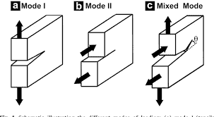
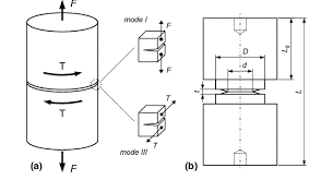
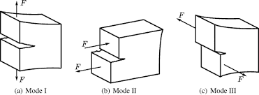
In optically anisotropic (birefringent) materials the change of the stress-optical path of a light ray is different along the directions of the two in-plane principal stresses $\sigma_1$ and $\sigma_2$. This change is given by Eq. (6.36) for the rays transmitted through the specimen and by Eq. (6.43) for the rays reflected from the rear face of the specimen. The plus (+) and minus (-) signs in these equations correspond to the two principal stresses. In such materials, two caustics are formed corresponding to the two principal stresses. Figure 6.17a, b presents the experimental double caustics at the crack tip formed by rays reflected from the rear face (a) and transmitted (b) through a specimen made of Polycarbonate of Bisphenol which is an optically anisotropic material. The specimen is loaded to opening mode.

Following the same procedure as in the case of optically isotropic materials presented previously, the opening-mode stress intensity factor $K_I$ can be determined from Eq. (6.61) using the transverse (t) or longitudinal (1) diameter $D_{t, l}$ of the caustic with the corresponding values of $\delta_t^{\max }$ or $\delta_l^{\max }$ (instead of $D$ and $\delta$, with $\mu=0$ ). The quantities $\delta_t^{\max }$ or $\delta_l^{\max }$ are functions of the anisotropy coefficient $\xi$ of the material. Figure 6.18 presents the variation of $\delta_t^{\max }$ and $\delta_l^{\max }$ versus $\xi$ for the transverse and longitudinal diameters of the caustic, respectively, for the outer and inner caustic.

物理代写|力学代写mechanics代考|The State of Stress Near the Crack Tip

The previous analysis of the method of caustics was based on the assumption that plane stress conditions apply in the neighborhood of the crack tip. The value of the stress-optical constant $c$ entered in Eqs. (6.55) and (6.60) for the determination of stress intensity factors $K_I, K_{I I}$ corresponds to plane stress conditions. However, the state of stress in the vicinity of the crack tip changes from plane strain very close to the tip to plane stress further away from the tip. Between these two regions, the stress field is three-dimensional. The value of $c$ changes when the state of stress changes from plane strain to plane stress. In order to use the correct value of $c$ for the determination of stress intensity factors $K_I, K_{I I}$ we should know the state of stress along the initial curve of the caustic.

It was established [3-10] that the state of stress becomes plane stress at distances $r$ from the crack tip larger than approximately half the specimen thickness. Thus, the radius of the initial curve of the caustic should be larger than half the specimen thickness $d, r_0>d / 2$. If $r_0<d / 2$ the initial curve lies in the region where the state of stress is three-dimensional and the plane stress value of $c$ does not apply. For the correct application of the method of caustics, the condition $r_0>d / 2$ should be satisfied. The radius of the initial curve $r_0$ can be determined from Eq. (6.51) after the determination of the stress intensity factor and the above condition should be checked. If the condition $r_0>d / 2$ is not satisfied the experiment should be considered invalid and should be repeated by changing the values of the dimensions of the optical setup and the applied loads.

力学代考

物理代写|力学代写mechanics代考|Anisotropic Materials

在光学各向异性（双折射）材料中，光线的应力光路的变化沿两个面内主应力的方向是不同的p1和p2. 这种变化由方程式给出。(6.36) 对于通过试样传输的射线和方程式。(6.43) 对于从试样背面反射的光线。这些方程式中的加号 (+) 和减号 (-) 对应于两个主应力。在此类材料中，对应于两个主应力形成两个焦散线。图 6.17a、b 显示了裂纹尖端处的实验性双焦散，由从背面 (a) 反射并透射 (b) 的光线穿过由双酚聚碳酸酯制成的样品（一种光学各向异性材料）形成。试样加载到打开模式。

按照与前面介绍的光学各向同性材料相同的程序，开模应力强度因子钾我可以从方程式确定。(6.61) 使用横向 (t) 或纵向 (1) 直径丁吨,升具有相应值的焦散d吨最大限度或者d升最大限度（代替丁和d， 和米=0). 数量d吨最大限度或者d升最大限度是各向异性系数的函数X的材料。图 6.18 显示了变化d吨最大限度和d升最大限度相对X对于焦散的横向和纵向直径，分别用于外部和内部焦散。

物理代写|力学代写mechanics代考|The State of Stress Near the Crack Tip

先前对焦散方法的分析是基于平面应力条件适用于裂纹尖端附近的假设。应力光学常数的值C输入方程式。(6.55) 和 (6.60) 用于确定应力强度因子钾我,钾我我对应于平面应力条件。然而，裂纹尖端附近的应力状态从非常靠近尖端的平面应变变为远离尖端的平面应力。在这两个区域之间，应力场是三维的。的价值C当应力状态从平面应变变为平面应力时发生变化。为了使用正确的值C用于确定应力强度因子钾我,钾我我我们应该知道沿焦散线初始曲线的应力状态。

已确定 [3-10] 应力状态在一定距离处变为平面应力r来自裂纹尖端的裂纹大于试样厚度的大约一半。因此，焦散的初始曲线半径应大于试样厚度的一半d,r0>d/2. 如果r0<d/2初始曲线位于应力状态为三维的区域，平面应力值为C不适用。为了正确应用焦散方法，条件r0>d/2应该是满意的。初始曲线的半径r0可以从方程式确定。(6.51) 应力强度因子测定后应检查上述条件。如果条件r0>d/2不满意实验应被视为无效，应通过更改光学设置的尺寸值和施加的负载来重复

统计代写请认准statistics-lab™. statistics-lab™为您的留学生涯保驾护航。

金融工程代写

金融工程是使用数学技术来解决金融问题。金融工程使用计算机科学、统计学、经济学和应用数学领域的工具和知识来解决当前的金融问题，以及设计新的和创新的金融产品。

非参数统计代写

非参数统计指的是一种统计方法，其中不假设数据来自于由少数参数决定的规定模型；这种模型的例子包括正态分布模型和线性回归模型。

广义线性模型代考

广义线性模型（GLM）归属统计学领域，是一种应用灵活的线性回归模型。该模型允许因变量的偏差分布有除了正态分布之外的其它分布。

术语 广义线性模型（GLM）通常是指给定连续和/或分类预测因素的连续响应变量的常规线性回归模型。它包括多元线性回归，以及方差分析和方差分析（仅含固定效应）。

有限元方法代写

有限元方法（FEM）是一种流行的方法，用于数值解决工程和数学建模中出现的微分方程。典型的问题领域包括结构分析、传热、流体流动、质量运输和电磁势等传统领域。

有限元是一种通用的数值方法，用于解决两个或三个空间变量的偏微分方程（即一些边界值问题）。为了解决一个问题，有限元将一个大系统细分为更小、更简单的部分，称为有限元。这是通过在空间维度上的特定空间离散化来实现的，它是通过构建对象的网格来实现的：用于求解的数值域，它有有限数量的点。边界值问题的有限元方法表述最终导致一个代数方程组。该方法在域上对未知函数进行逼近。[1] 然后将模拟这些有限元的简单方程组合成一个更大的方程系统，以模拟整个问题。然后，有限元通过变化微积分使相关的误差函数最小化来逼近一个解决方案。

tatistics-lab作为专业的留学生服务机构，多年来已为美国、英国、加拿大、澳洲等留学热门地的学生提供专业的学术服务，包括但不限于Essay代写，Assignment代写，Dissertation代写，Report代写，小组作业代写，Proposal代写，Paper代写，Presentation代写，计算机作业代写，论文修改和润色，网课代做，exam代考等等。写作范围涵盖高中，本科，研究生等海外留学全阶段，辐射金融，经济学，会计学，审计学，管理学等全球99%专业科目。写作团队既有专业英语母语作者，也有海外名校硕博留学生，每位写作老师都拥有过硬的语言能力，专业的学科背景和学术写作经验。我们承诺100%原创，100%专业，100%准时，100%满意。

随机分析代写

随机微积分是数学的一个分支，对随机过程进行操作。它允许为随机过程的积分定义一个关于随机过程的一致的积分理论。这个领域是由日本数学家伊藤清在第二次世界大战期间创建并开始的。

时间序列分析代写

随机过程，是依赖于参数的一组随机变量的全体，参数通常是时间。 随机变量是随机现象的数量表现，其时间序列是一组按照时间发生先后顺序进行排列的数据点序列。通常一组时间序列的时间间隔为一恒定值（如1秒，5分钟，12小时，7天，1年），因此时间序列可以作为离散时间数据进行分析处理。研究时间序列数据的意义在于现实中，往往需要研究某个事物其随时间发展变化的规律。这就需要通过研究该事物过去发展的历史记录，以得到其自身发展的规律。

回归分析代写

多元回归分析渐进（Multiple Regression Analysis Asymptotics）属于计量经济学领域，主要是一种数学上的统计分析方法，可以分析复杂情况下各影响因素的数学关系，在自然科学、社会和经济学等多个领域内应用广泛。

MATLAB代写

MATLAB 是一种用于技术计算的高性能语言。它将计算、可视化和编程集成在一个易于使用的环境中，其中问题和解决方案以熟悉的数学符号表示。典型用途包括：数学和计算算法开发建模、仿真和原型制作数据分析、探索和可视化科学和工程图形应用程序开发，包括图形用户界面构建MATLAB 是一个交互式系统，其基本数据元素是一个不需要维度的数组。这使您可以解决许多技术计算问题，尤其是那些具有矩阵和向量公式的问题，而只需用 C 或 Fortran 等标量非交互式语言编写程序所需的时间的一小部分。MATLAB 名称代表矩阵实验室。MATLAB 最初的编写目的是提供对由 LINPACK 和 EISPACK 项目开发的矩阵软件的轻松访问，这两个项目共同代表了矩阵计算软件的最新技术。MATLAB 经过多年的发展，得到了许多用户的投入。在大学环境中，它是数学、工程和科学入门和高级课程的标准教学工具。在工业领域，MATLAB 是高效研究、开发和分析的首选工具。MATLAB 具有一系列称为工具箱的特定于应用程序的解决方案。对于大多数 MATLAB 用户来说非常重要，工具箱允许您学习和应用专业技术。工具箱是 MATLAB 函数（M 文件）的综合集合，可扩展 MATLAB 环境以解决特定类别的问题。可用工具箱的领域包括信号处理、控制系统、神经网络、模糊逻辑、小波、仿真等。

R语言代写	问卷设计与分析代写
PYTHON代写	回归分析与线性模型代写
MATLAB代写	方差分析与试验设计代写
STATA代写	机器学习/统计学习代写
SPSS代写	计量经济学代写
EVIEWS代写	时间序列分析代写
EXCEL代写	深度学习代写
SQL代写	各种数据建模与可视化代写

如果你也在 怎样代写力学mechanics这个学科遇到相关的难题，请随时右上角联系我们的24/7代写客服。

力学是物理学的一个分支，主要研究能量和力以及它们与物体的平衡、变形或运动的关系。

statistics-lab™ 为您的留学生涯保驾护航 在代写力学mechanics方面已经树立了自己的口碑, 保证靠谱, 高质且原创的统计Statistics代写服务。我们的专家在代写力学mechanics代写方面经验极为丰富，各种代写力学mechanics相关的作业也就用不着说。

我们提供的力学mechanics及其相关学科的代写，服务范围广, 其中包括但不限于:

• Statistical Inference 统计推断
• Statistical Computing 统计计算
• Advanced Probability Theory 高等概率论
• Advanced Mathematical Statistics 高等数理统计学
• (Generalized) Linear Models 广义线性模型
• Statistical Machine Learning 统计机器学习
• Longitudinal Data Analysis 纵向数据分析
• Foundations of Data Science 数据科学基础

物理代写|力学代写mechanics代考|Opening-Mode Loading

Consider a transparent specimen illuminated by a parallel light beam and a screen at a distance $z_0$ downstream from the specimen placed parallel to the plane of the specimen (Fig. 6.9). A point $P$ on the specimen is imaged at point $P^{\prime}$ on the screen. It is assumed that the slopes of the surface are small and the distance $z_0$ is large compared to the change of the specimen thickness due to loading.

For the case of a transparent specimen the mapping equation of point $P$ to point $P^{\prime}$, according to Eq. $(6.5)$, is given by
$$
\begin{aligned}
& W_x=x-z_0 \frac{\partial(\Delta s)}{\partial x} \
& W_y=y-z_0 \frac{\partial(\Delta s)}{\partial y}
\end{aligned}
$$
where $\Delta s$ is the change of the optical path of a ray passing through the specimen due to loading.

For an optically inert material, $\Delta s$ is given by Eq. (6.37) for the light rays traversing the specimen and by Eq. (6.44) for the light rays reflected from the rear face of the transparent specimen. For the rays reflected from the front face of the specimen the stress-optical constant $c_t$ in Eq. (6.37) should be replaced by the ratio $v / E(v$ is the Poisson’s ratio and $E$ is the modulus of elasticity). For all three cases of light rays traversing the specimen, reflected from the rear face or from the front face of the specimen the transformation Fq. (6.45) applies with different valnes of the stress-optical constant $\mathrm{c}$, which takes the values $c_t, 2 c_r$, or $v / E$, respectively.

The singular polar stresses at the tip of the crack for opening-mode loading governed by value of the stress intensity factor $K_I$ are given by [2]
$$
\begin{aligned}
\sigma_r & =\frac{K_I}{4 \sqrt{2 \pi r}}\left(5 \cos \frac{\theta}{2}-\cos \frac{3 \theta}{2}\right) \
\sigma_\theta & =\frac{K_I}{4 \sqrt{2 \pi r}}\left(3 \cos \frac{\theta}{2}+\cos \frac{3 \theta}{2}\right) \
\sigma_{r \theta} & =\frac{K_I}{4 \sqrt{2 \pi r}}\left(\sin \frac{\theta}{2}+\sin \frac{3 \theta}{2}\right)
\end{aligned}
$$
where $r$ is the distance from the origin of the coordinate system placed at the crack tip and $\theta$ is the polar angle.

物理代写|力学代写mechanics代考|Mixed-Mode Loading

When the applied loads are not normal to the crack plane mixed-mode conditions apply in the vicinity of the crack tip. The singular stresses in polar coordinates are given in terms of the opening-mode $K_I$ and sliding-mode $K_{I I}$ stress intensity factors by the following equations [2]
$$
\begin{aligned}
\sigma_r & =\frac{K_I}{4 \sqrt{2 \pi r}}\left(5 \cos \frac{\theta}{2}-\cos \frac{3 \theta}{2}\right)+\frac{K_{I I}}{4 \sqrt{2 \pi r}}\left(-5 \sin \frac{\theta}{2}+3 \sin \frac{3 \theta}{2}\right) \
\sigma_\theta & =\frac{K_I}{4 \sqrt{2 \pi r}}\left(3 \cos \frac{\theta}{2}+\cos \frac{3 \theta}{2}\right)+\frac{K_{I I}}{4 \sqrt{2 \pi r}}\left(-3 \sin \frac{\theta}{2}-3 \sin \frac{3 \theta}{2}\right)
\end{aligned}
$$ $$
\sigma_{r \theta}=\frac{K_I}{4 \sqrt{2 \pi r}}\left(\sin \frac{\theta}{2}+\sin \frac{3 \theta}{2}\right)+\frac{K_{I I}}{4 \sqrt{2 \pi r}}\left(\cos \frac{\theta}{2}+3 \cos \frac{3 \theta}{2}\right)
$$
The sum of the stresses $\sigma_r$ and $\sigma_\theta$ is given by
$$
\sigma_r+\sigma_\theta=\frac{2 K_I}{\sqrt{2 \pi r}} \cos \frac{\theta}{2}-\frac{2 K_{I I}}{\sqrt{2 \pi r}} \sin \frac{\theta}{2}
$$
Working as in the previous case of opening-mode loading, we obtain the following equations of the caustic
$$
\begin{aligned}
& W_x=x^{\prime}=r_0\left[\cos \theta+\frac{2}{3}\left(1+\mu^2\right)^{-1 / 2} \cos \frac{3 \theta}{2}-\frac{2}{3} \mu\left(1+\mu^2\right)^{-1 / 2} \sin \frac{3 \theta}{2}\right] \
& W_y=y^{\prime}=r_0\left[\sin \theta+\frac{2}{3}\left(1+\mu^2\right)^{-1 / 2} \sin \frac{3 \theta}{2}+\frac{2}{3} \mu\left(1+\mu^2\right)^{-1 / 2} \cos \frac{3 \theta}{2}\right]
\end{aligned}
$$
With
$$
r=r_0=\left(\frac{3 z_0 d c K_I}{2 \sqrt{2 \pi}}\right)^{2 / 5}\left(1+\mu^2\right)^{1 / 5}, \quad \mu=K_{I I} / K_I
$$
The stress intensity factors $K_I$ and $K_{I I}$ are obtained as
$$
K_I=\frac{1.671}{z_0 d c m^{3 / 2}}\left(\frac{D}{\delta}\right)^{5 / 2} \frac{1}{\sqrt{1+\mu^2}}, \quad K_{I I}=\mu K_I
$$
The ratio $D / \delta$ takes either of the values $r_0=D_t / \delta_t, D_l^{\max } / \delta_l^{\max }, D_l^{\min } / \delta_l^{\min }$, where $D_l^{\max }$ and $D_l^{\min }$ are the maximum and minimum diameters of the caustic along the cräck planee and $D_t$ is the transverse (perpendiculär to the crack plané) dianeter of the caustic at the crack tip. The quantities $\delta_l^{\max }$ and $\delta_l^{\min }$ depend on the value of 4. For opening-mode loading $\delta_t=3.16, \delta_l^{\max }=\delta_l^{\min }=3$. Figure 6.13 presents the geometrical construction of the caustic for $\mu=0.5$. In Fig. 6.14 four caustics corresponding to $\mu=0,0.25,1.0$ and $\infty$ are shown. The values of $\mu=0$ and $\infty$ refer to the cases of pure tension (opening-mode loading) and pure shear (sliding-mode loading), respectively. Note that the caustic for $\mu=0$ is symmetric with respect to the $x$-axis, while the other caustics for $\mu \neq 0$ do not present a symmetry. Figure 6.15 presents the variation of the quantities $\delta_t=D_t / r_0, \delta_l^{\max }=D_l^{\max } / r_0, \delta_l^{\min }=D_l^{\min } / r_0$ versus $\mu$. Note that for $\mu=0 . \delta_t=3.16$, while for $\mu=1, \delta_t=2.99$. The variation of the ratio $\left(D_l^{\max }-D_l^{\min }\right) / D_l^{\max }$ versus $\mu$ is shown in Fig. 6.16.

力学代考

物理代写|力学代写mechanics代考|Opening-Mode Loading

考虑一个由平行光束和远处的屏幕照亮的透明标本 $z_0$ 样品下游平行于样品平面放置 (图 6.9) 。一点 $P$ 标本上的成像点 $P^{\prime}$ 屏幕上。假设表面的斜率很小并且距离 $z_0$ 与载荷引起的试样厚度变化相比，它很大。
对于透明样品的情况，点的映射方程 $P$ 指向 $P^{\prime}$ ，根据方程式。 (6.5)，是（谁) 给的
$$
W_x=x-z_0 \frac{\partial(\Delta s)}{\partial x} \quad W_y=y-z_0 \frac{\partial(\Delta s)}{\partial y}
$$
在哪里 $\Delta s$ 是由于载荷引起的穿过试样的光线光路的变化。
对于光学惰性材料， $\Delta s$ 由方程式给出。(6.37) 对于穿过样品的光线和通过 Eq. (6.44) 对于从透明样品背 面反射的光线。对于从试样正面反射的光线，应力光学常数 $c_t$ 在等式中 (6.37) 应替换为比率 $v / E(v$ 是泊 松比和 $E$ 是弹性模量）。对于穿过样本的所有三种情况，从样本的背面或从样本的正面反射的变换 $F q$ 。 (6.45) 适用于应力光学常数的不同值c, 它取值 $c_t, 2 c_r$ ，或者 $v / E$ ，分别。
由应力强度因子的值控制的开模加载裂纹尖端的奇异极性应力 $K_I$ 由 [2] 给出
$$
\sigma_r=\frac{K_I}{4 \sqrt{2 \pi r}}\left(5 \cos \frac{\theta}{2}-\cos \frac{3 \theta}{2}\right) \sigma_\theta=\frac{K_I}{4 \sqrt{2 \pi r}}\left(3 \cos \frac{\theta}{2}+\cos \frac{3 \theta}{2}\right) \sigma_{r \theta}=\frac{K_I}{4 \sqrt{2 \pi r}}(\sin
$$
在哪里 $r$ 是距位于裂纹尖端的坐标系原点的距离， $\theta$ 是极角。

物理代写|力学代写mechanics代考|Mixed-Mode Loading

当施加的载荷不垂直于裂纹平面时，混合模式条件适用于裂纹尖端附近。极坐标中的奇异应力以开模形 式给出 $K_I$ 和滑动模式 $K_{I I}$ 应力强度因子由以下方程 [2]
$$
\begin{gathered}
\sigma_r=\frac{K_I}{4 \sqrt{2 \pi r}}\left(5 \cos \frac{\theta}{2}-\cos \frac{3 \theta}{2}\right)+\frac{K_{I I}}{4 \sqrt{2 \pi r}}\left(-5 \sin \frac{\theta}{2}+3 \sin \frac{3 \theta}{2}\right) \sigma_\theta=\frac{K_I}{4 \sqrt{2 \pi r}}(3 \cos \
\sigma_{r \theta}=\frac{K_I}{4 \sqrt{2 \pi r}}\left(\sin \frac{\theta}{2}+\sin \frac{3 \theta}{2}\right)+\frac{K_{I I}}{4 \sqrt{2 \pi r}}\left(\cos \frac{\theta}{2}+3 \cos \frac{3 \theta}{2}\right)
\end{gathered}
$$
应力总和 $\sigma_r$ 和 $\sigma_\theta$ 是 (谁) 给的
$$
\sigma_r+\sigma_\theta=\frac{2 K_I}{\sqrt{2 \pi r}} \cos \frac{\theta}{2}-\frac{2 K_{I I}}{\sqrt{2 \pi r}} \sin \frac{\theta}{2}
$$
与前面的开放模式加载情况一样，我们得到以下焦散方程
$$
W_x=x^{\prime}=r_0\left[\cos \theta+\frac{2}{3}\left(1+\mu^2\right)^{-1 / 2} \cos \frac{3 \theta}{2}-\frac{2}{3} \mu\left(1+\mu^2\right)^{-1 / 2} \sin \frac{3 \theta}{2}\right] \quad W_y=y^{\prime}=r_0
$$
和
$$
r=r_0=\left(\frac{3 z_0 d c K_I}{2 \sqrt{2 \pi}}\right)^{2 / 5}\left(1+\mu^2\right)^{1 / 5}, \quad \mu=K_{I I} / K_I
$$
应力强度因子 $K_I$ 和 $K_{I I}$ 获得为
$$
K_I=\frac{1.671}{z_0 d c m^{3 / 2}}\left(\frac{D}{\delta}\right)^{5 / 2} \frac{1}{\sqrt{1+\mu^2}}, \quad K_{I I}=\mu K_I
$$
比例 $D / \delta$ 取任一个值 $r_0=D_t / \delta_t, D_l^{\max } / \delta_l^{\max }, D_l^{\min } / \delta_l^{\min }$ ，在哪里 $D_l^{\max }$ 和 $D_l^{\min }$ 是焦散沿裂纹平 面的最大和最小直径，并且 $D_t$ 是裂纹尖端焦散的横向 (垂直于裂纹平面) 直径。数量 $\delta_l^{\max }$ 和 $\delta_l^{\min }$ 取决 于4的值。对于开放模式加载 $\delta_t=3.16, \delta_l^{\max }=\delta_l^{\min }=3$. 图 6.13 展示了焦散的几何构造 $\mu=0.5$. 在图 6.14 中，四个焦散对应于 $\mu=0,0.25,1.0$ 和 $\infty$ 显示。的价值观 $\mu=0$ 和 $\infty$ 分别指纯张力（开模 加载) 和纯剪切 (滑模加载) 的情况。请注意，苛性碱 $\mu=0$ 是关于对称的 $x$-轴，而其他焦散 $\mu \neq 0$ 不 呈现对称性。图 6.15 显示了数量的变化 $\delta_t=D_t / r_0, \delta_l^{\max }=D_l^{\max } / r_0, \delta_l^{\min }=D_l^{\min } / r_0$ 相对 $\mu$. 请 注意，对于 $\mu=0 . \delta_t=3.16$, 而对于 $\mu=1, \delta_t=2.99$. 比率的变化 $\left(D_l^{\max }-D_l^{\min }\right) / D_l^{\max }$ 相对 $\mu$ 如图 6.16 所示。

统计代写请认准statistics-lab™. statistics-lab™为您的留学生涯保驾护航。

金融工程代写

金融工程是使用数学技术来解决金融问题。金融工程使用计算机科学、统计学、经济学和应用数学领域的工具和知识来解决当前的金融问题，以及设计新的和创新的金融产品。

非参数统计代写

非参数统计指的是一种统计方法，其中不假设数据来自于由少数参数决定的规定模型；这种模型的例子包括正态分布模型和线性回归模型。

广义线性模型代考

广义线性模型（GLM）归属统计学领域，是一种应用灵活的线性回归模型。该模型允许因变量的偏差分布有除了正态分布之外的其它分布。

术语 广义线性模型（GLM）通常是指给定连续和/或分类预测因素的连续响应变量的常规线性回归模型。它包括多元线性回归，以及方差分析和方差分析（仅含固定效应）。

有限元方法代写

有限元方法（FEM）是一种流行的方法，用于数值解决工程和数学建模中出现的微分方程。典型的问题领域包括结构分析、传热、流体流动、质量运输和电磁势等传统领域。

有限元是一种通用的数值方法，用于解决两个或三个空间变量的偏微分方程（即一些边界值问题）。为了解决一个问题，有限元将一个大系统细分为更小、更简单的部分，称为有限元。这是通过在空间维度上的特定空间离散化来实现的，它是通过构建对象的网格来实现的：用于求解的数值域，它有有限数量的点。边界值问题的有限元方法表述最终导致一个代数方程组。该方法在域上对未知函数进行逼近。[1] 然后将模拟这些有限元的简单方程组合成一个更大的方程系统，以模拟整个问题。然后，有限元通过变化微积分使相关的误差函数最小化来逼近一个解决方案。

tatistics-lab作为专业的留学生服务机构，多年来已为美国、英国、加拿大、澳洲等留学热门地的学生提供专业的学术服务，包括但不限于Essay代写，Assignment代写，Dissertation代写，Report代写，小组作业代写，Proposal代写，Paper代写，Presentation代写，计算机作业代写，论文修改和润色，网课代做，exam代考等等。写作范围涵盖高中，本科，研究生等海外留学全阶段，辐射金融，经济学，会计学，审计学，管理学等全球99%专业科目。写作团队既有专业英语母语作者，也有海外名校硕博留学生，每位写作老师都拥有过硬的语言能力，专业的学科背景和学术写作经验。我们承诺100%原创，100%专业，100%准时，100%满意。

随机分析代写

随机微积分是数学的一个分支，对随机过程进行操作。它允许为随机过程的积分定义一个关于随机过程的一致的积分理论。这个领域是由日本数学家伊藤清在第二次世界大战期间创建并开始的。

时间序列分析代写

随机过程，是依赖于参数的一组随机变量的全体，参数通常是时间。 随机变量是随机现象的数量表现，其时间序列是一组按照时间发生先后顺序进行排列的数据点序列。通常一组时间序列的时间间隔为一恒定值（如1秒，5分钟，12小时，7天，1年），因此时间序列可以作为离散时间数据进行分析处理。研究时间序列数据的意义在于现实中，往往需要研究某个事物其随时间发展变化的规律。这就需要通过研究该事物过去发展的历史记录，以得到其自身发展的规律。

回归分析代写

多元回归分析渐进（Multiple Regression Analysis Asymptotics）属于计量经济学领域，主要是一种数学上的统计分析方法，可以分析复杂情况下各影响因素的数学关系，在自然科学、社会和经济学等多个领域内应用广泛。

MATLAB代写

MATLAB 是一种用于技术计算的高性能语言。它将计算、可视化和编程集成在一个易于使用的环境中，其中问题和解决方案以熟悉的数学符号表示。典型用途包括：数学和计算算法开发建模、仿真和原型制作数据分析、探索和可视化科学和工程图形应用程序开发，包括图形用户界面构建MATLAB 是一个交互式系统，其基本数据元素是一个不需要维度的数组。这使您可以解决许多技术计算问题，尤其是那些具有矩阵和向量公式的问题，而只需用 C 或 Fortran 等标量非交互式语言编写程序所需的时间的一小部分。MATLAB 名称代表矩阵实验室。MATLAB 最初的编写目的是提供对由 LINPACK 和 EISPACK 项目开发的矩阵软件的轻松访问，这两个项目共同代表了矩阵计算软件的最新技术。MATLAB 经过多年的发展，得到了许多用户的投入。在大学环境中，它是数学、工程和科学入门和高级课程的标准教学工具。在工业领域，MATLAB 是高效研究、开发和分析的首选工具。MATLAB 具有一系列称为工具箱的特定于应用程序的解决方案。对于大多数 MATLAB 用户来说非常重要，工具箱允许您学习和应用专业技术。工具箱是 MATLAB 函数（M 文件）的综合集合，可扩展 MATLAB 环境以解决特定类别的问题。可用工具箱的领域包括信号处理、控制系统、神经网络、模糊逻辑、小波、仿真等。

R语言代写	问卷设计与分析代写
PYTHON代写	回归分析与线性模型代写
MATLAB代写	方差分析与试验设计代写
STATA代写	机器学习/统计学习代写
SPSS代写	计量经济学代写
EVIEWS代写	时间序列分析代写
EXCEL代写	深度学习代写
SQL代写	各种数据建模与可视化代写

如果你也在 怎样代写力学mechanics这个学科遇到相关的难题，请随时右上角联系我们的24/7代写客服。

力学是物理学的一个分支，主要研究能量和力以及它们与物体的平衡、变形或运动的关系。

statistics-lab™ 为您的留学生涯保驾护航 在代写力学mechanics方面已经树立了自己的口碑, 保证靠谱, 高质且原创的统计Statistics代写服务。我们的专家在代写力学mechanics代写方面经验极为丰富，各种代写力学mechanics相关的作业也就用不着说。

我们提供的力学mechanics及其相关学科的代写，服务范围广, 其中包括但不限于:

• Statistical Inference 统计推断
• Statistical Computing 统计计算
• Advanced Probability Theory 高等概率论
• Advanced Mathematical Statistics 高等数理统计学
• (Generalized) Linear Models 广义线性模型
• Statistical Machine Learning 统计机器学习
• Longitudinal Data Analysis 纵向数据分析
• Foundations of Data Science 数据科学基础

物理代写|力学代写mechanics代考|Mathematical Analysis of Moiré Fringes

Consider two indexed families of curves representing the specimen and reference gratings expressed by the indicial equations
$$
S(x, y)=k, R(x, y)=l(k, l=\pm 1, \pm 2, \ldots)
$$
When the two gratings are superposed the resulting moiré pattern is expressed by an indexed family of curves $M(x, y)=m(m=\pm 1, \pm 2, \ldots)$. The moiré fringes are the diagonals of the curvilinear quadrangles formed by the intersection of the curves of the two gratings. They are expressed by the following indicial equation (Fig. 3.5).
$$
k \pm l=m
$$
Points $E, F, G, H, \ldots$ of Fig. $3.5$ correspond to the moiré pattern for which $(k$ $-l)=$ constant, while points $A, B, C, D, \ldots$ of Fig. $3.5$ correspond to the moiré pattern for which $(k+l)=$ constant. The moiré fringes for which the equation $(k-l)$ $=m$ applies is called the subtractive moirépattern, while the moiré fringes for which the equation $(k+l)=m$ applies is called the additive moirépattern. As we mentioned previously, the effective or visible moiré pattern is the pattern with the longest intefringe spacing or the shortest diagonals of the individual quadrangles. The effective moire pattern in Fig. $3.5$ is the pattern containing the fringe $E F G H$ and belongs to the subtractive moiré pattern.

Equation (3.7) indicates that the moiré pattern is the result of adding or subtracting two functions that are expressed parametrically. The moiré pattern can also be considered as a family of parametric curves. Knowledge of any two of the three families of curves allows the determination of the third. In displacement analysis, one family is the master grating and a second is the moiré fringes. The third family is the deformed specimen grating from which the displacements of the specimen are measured.
The effective moiré pattern may change from subtractive type to additive type and vice versa. The boundary between the two moire types is the region in which the individual quadrangles are squares. It is called commutation moiré boundary or simply moiré boundary.

物理代写|力学代写mechanics代考|Relationships Between Line Grating and Moiré Fringes

Line gratings are mostly used in experimental mechanics. In this section, we will develop the relationships between the pitches and relative inclination of two lines gratings and the spacing and inclination of the resulting moiré fringes. The moiré fringes are straight lines that coincide with the diagonals of the rhombuses formed by the intersections of the lines of the two gratings. We will use the general method presented previously known as geometric approach.

Consider two lines gratings $S(x, y)=k$ and $R(x, y)=l$ of pitches, $p$ and $p_1=p(1$ $+\lambda$ ), respectively, referred to a system of Cartesian coordinates $O x y$ (Fig. 3.7). The lines of the grating $S(x, y)$ are parallel to the $x$-axis, while the lines of the grating $R(x$, $y$ ) make an angle $\theta$ with the $x$-axis. The line $k=0$ of grating $S(x, y)$ and the line $l=$ 0 of grating $R(x, y)$ pass through the origin $O$ of the system $O x y$.
The equations of the two gratings are expressed by
$$
\begin{gathered}
S(x, y)=k=\frac{y}{p} \
R(x, y)=1=\frac{y \cos \theta-x \sin \theta}{p(1+\lambda)}
\end{gathered}
$$

From Eq. (3.7) we obtain for the equation of the fringes of the subtractive moiré pattern
$$
\frac{y}{p}-\frac{y \cos \theta-x \sin \theta}{p(1+\lambda)}=m
$$
or after rearranging the terms
$$
y\left[\frac{\cos \theta-(1+\lambda)}{\sin \theta}\right]+\frac{m p(1+\lambda)}{\sin \theta}=x
$$
The moiré fringes are straight lines with an angle of inclination $\varphi$ with the $x$-axis and at a distance $f$ (interfringe spacing) between them. Their equation can also be obtained from Eq. (3.19) by replacing $\theta$ with $\varphi$, and $p(1+\lambda)$ with $f$. We obtain
$$
y \cot \varphi-\frac{m f}{\sin \varphi}=x
$$

力学代考

物理代写|力学代写mechanics代考|Mathematical Analysis of Moiré Fringes

考虑代表试样和参考光栅的两个索引曲线族，由索引方程表示
$$
S(x, y)=k, R(x, y)=l(k, l=\pm 1, \pm 2, \ldots)
$$
个光栅的曲线相交形成的曲线四边形的对角线。它们由以下公式表示 (图 3.5) 。
$$
k \pm l=m
$$
积分 $E, F, G, H, \ldots$ 图的 $3.5$ 对应于莫尔图案 $(k-l)=$ 常数，而点 $A, B, C, D, \ldots$ 图的 $3.5$ 对应于莫尔图案 $(k+l)=$ 持续的。等式所对应的莫尔条纹 $(k-l)=m$ 适用的莫尔条纹称为减法莫尔条纹，而莫尔条纹
$(k+l)=m$ 应用称为加性莫尔图案。正如我们之前提到的，有效或可见的莫尔图案是具有最长的干涉条纹间距 或各个四边形的最短对角线的图案。图 1 中的有效云纹图案 $3.5$ 是包含条纹的图案 $E F G H$ 属于减法莫尔纹。
等式 (3.7) 表明莫尔图案是两个以参数表示的函数相加或相减的结果。莫尔图案也可以被认为是参数曲线族。了解 三个曲线族中的任何两个曲线可以确定第三个曲线族。在位移分析中，一个族是主光栅，第二个族是莫尔条纹。 第三类是变形的试样光栅，从中测量试样的位移。
有效的莫尔图案可以从减法类型变为加法类型，反之亦然。两种云纹类型之间的边界是各个四边形为正方形的区 域。它被称为换向莫尔边界或简称为莫尔边界。

物理代写|力学代写mechanics代考|Relationships Between Line Grating and Moiré Fringes

线光栅主要用于实验力学。在本节中，我们将研究两条线光栅的间距和相对倾斜度以及由此产生的莫尔条纹的间 距和倾斜度之间的关系。莫尔条纹是与两个光栅的线相交形成的菱形的对角线重合的直线。我们将使用前面介绍 的一般方法，即几何方法。
考虑两条线光栅 $S(x, y)=k$ 和 $R(x, y)=l$ 球场， $p$ 和 $p_1=p(1+\lambda)$ 分别表示笛卡尔坐标系 $O x y$ (图 3.7) 。 光栅的线条 $S(x, y)$ 平行于 $x$-轴，而光栅的线 $R(x, y)$ 做一个角度 $\theta$ 与 $x$-轴。线 $k=0$ 光栅的 $S(x, y)$ 和线 $l=0$ 个 光栅 $R(x, y)$ 穿越原点 $O$ 系统的 $O x y$.
两个光栅的方程表示为
$$
S(x, y)=k=\frac{y}{p} R(x, y)=1=\frac{y \cos \theta-x \sin \theta}{p(1+\lambda)}
$$
从方程式。(3.7) 我们得到减法莫尔条纹的方程
$$
\frac{y}{p}-\frac{y \cos \theta-x \sin \theta}{p(1+\lambda)}=m
$$
或重新排列条款后
$$
y\left[\frac{\cos \theta-(1+\lambda)}{\sin \theta}\right]+\frac{m p(1+\lambda)}{\sin \theta}=x
$$
莫尔条纹是具有倾斜角的直线 $\varphi$ 与 $x$-轴和远处 $f$ (干涉间距) 。他们的方程也可以从方程得到。(3.19) 通过替换 $\theta$ 和 $\varphi$ ，和 $p(1+\lambda)$ 和 $f$. 我们获得
$$
y \cot \varphi-\frac{m f}{\sin \varphi}=x
$$

统计代写请认准statistics-lab™. statistics-lab™为您的留学生涯保驾护航。

金融工程代写

金融工程是使用数学技术来解决金融问题。金融工程使用计算机科学、统计学、经济学和应用数学领域的工具和知识来解决当前的金融问题，以及设计新的和创新的金融产品。

非参数统计代写

非参数统计指的是一种统计方法，其中不假设数据来自于由少数参数决定的规定模型；这种模型的例子包括正态分布模型和线性回归模型。

广义线性模型代考

广义线性模型（GLM）归属统计学领域，是一种应用灵活的线性回归模型。该模型允许因变量的偏差分布有除了正态分布之外的其它分布。

术语 广义线性模型（GLM）通常是指给定连续和/或分类预测因素的连续响应变量的常规线性回归模型。它包括多元线性回归，以及方差分析和方差分析（仅含固定效应）。

有限元方法代写

有限元方法（FEM）是一种流行的方法，用于数值解决工程和数学建模中出现的微分方程。典型的问题领域包括结构分析、传热、流体流动、质量运输和电磁势等传统领域。

有限元是一种通用的数值方法，用于解决两个或三个空间变量的偏微分方程（即一些边界值问题）。为了解决一个问题，有限元将一个大系统细分为更小、更简单的部分，称为有限元。这是通过在空间维度上的特定空间离散化来实现的，它是通过构建对象的网格来实现的：用于求解的数值域，它有有限数量的点。边界值问题的有限元方法表述最终导致一个代数方程组。该方法在域上对未知函数进行逼近。[1] 然后将模拟这些有限元的简单方程组合成一个更大的方程系统，以模拟整个问题。然后，有限元通过变化微积分使相关的误差函数最小化来逼近一个解决方案。

tatistics-lab作为专业的留学生服务机构，多年来已为美国、英国、加拿大、澳洲等留学热门地的学生提供专业的学术服务，包括但不限于Essay代写，Assignment代写，Dissertation代写，Report代写，小组作业代写，Proposal代写，Paper代写，Presentation代写，计算机作业代写，论文修改和润色，网课代做，exam代考等等。写作范围涵盖高中，本科，研究生等海外留学全阶段，辐射金融，经济学，会计学，审计学，管理学等全球99%专业科目。写作团队既有专业英语母语作者，也有海外名校硕博留学生，每位写作老师都拥有过硬的语言能力，专业的学科背景和学术写作经验。我们承诺100%原创，100%专业，100%准时，100%满意。

随机分析代写

随机微积分是数学的一个分支，对随机过程进行操作。它允许为随机过程的积分定义一个关于随机过程的一致的积分理论。这个领域是由日本数学家伊藤清在第二次世界大战期间创建并开始的。

时间序列分析代写

随机过程，是依赖于参数的一组随机变量的全体，参数通常是时间。 随机变量是随机现象的数量表现，其时间序列是一组按照时间发生先后顺序进行排列的数据点序列。通常一组时间序列的时间间隔为一恒定值（如1秒，5分钟，12小时，7天，1年），因此时间序列可以作为离散时间数据进行分析处理。研究时间序列数据的意义在于现实中，往往需要研究某个事物其随时间发展变化的规律。这就需要通过研究该事物过去发展的历史记录，以得到其自身发展的规律。

回归分析代写

多元回归分析渐进（Multiple Regression Analysis Asymptotics）属于计量经济学领域，主要是一种数学上的统计分析方法，可以分析复杂情况下各影响因素的数学关系，在自然科学、社会和经济学等多个领域内应用广泛。

MATLAB代写

MATLAB 是一种用于技术计算的高性能语言。它将计算、可视化和编程集成在一个易于使用的环境中，其中问题和解决方案以熟悉的数学符号表示。典型用途包括：数学和计算算法开发建模、仿真和原型制作数据分析、探索和可视化科学和工程图形应用程序开发，包括图形用户界面构建MATLAB 是一个交互式系统，其基本数据元素是一个不需要维度的数组。这使您可以解决许多技术计算问题，尤其是那些具有矩阵和向量公式的问题，而只需用 C 或 Fortran 等标量非交互式语言编写程序所需的时间的一小部分。MATLAB 名称代表矩阵实验室。MATLAB 最初的编写目的是提供对由 LINPACK 和 EISPACK 项目开发的矩阵软件的轻松访问，这两个项目共同代表了矩阵计算软件的最新技术。MATLAB 经过多年的发展，得到了许多用户的投入。在大学环境中，它是数学、工程和科学入门和高级课程的标准教学工具。在工业领域，MATLAB 是高效研究、开发和分析的首选工具。MATLAB 具有一系列称为工具箱的特定于应用程序的解决方案。对于大多数 MATLAB 用户来说非常重要，工具箱允许您学习和应用专业技术。工具箱是 MATLAB 函数（M 文件）的综合集合，可扩展 MATLAB 环境以解决特定类别的问题。可用工具箱的领域包括信号处理、控制系统、神经网络、模糊逻辑、小波、仿真等。

R语言代写	问卷设计与分析代写
PYTHON代写	回归分析与线性模型代写
MATLAB代写	方差分析与试验设计代写
STATA代写	机器学习/统计学习代写
SPSS代写	计量经济学代写
EVIEWS代写	时间序列分析代写
EXCEL代写	深度学习代写
SQL代写	各种数据建模与可视化代写

如果你也在 怎样代写力学mechanics这个学科遇到相关的难题，请随时右上角联系我们的24/7代写客服。

力学是物理学的一个分支，主要研究能量和力以及它们与物体的平衡、变形或运动的关系。

statistics-lab™ 为您的留学生涯保驾护航 在代写力学mechanics方面已经树立了自己的口碑, 保证靠谱, 高质且原创的统计Statistics代写服务。我们的专家在代写力学mechanics代写方面经验极为丰富，各种代写力学mechanics相关的作业也就用不着说。

我们提供的力学mechanics及其相关学科的代写，服务范围广, 其中包括但不限于:

• Statistical Inference 统计推断
• Statistical Computing 统计计算
• Advanced Probability Theory 高等概率论
• Advanced Mathematical Statistics 高等数理统计学
• (Generalized) Linear Models 广义线性模型
• Statistical Machine Learning 统计机器学习
• Longitudinal Data Analysis 纵向数据分析
• Foundations of Data Science 数据科学基础

物理代写|力学代写mechanics代考|Terminology

The moiré phenomenon occurs whenever a repetitive structure, such as a mess, is overlaid with another such structure. The two structures need not be identical. The effect is observed in everyday life. Examples include the pattern seen through two rows of a mesh, or picket fence from a distance, layers of window screens, or coarse textiles. Before studying the moiré effect we will define a few terms that are needed for its understanding.

The basic element in the moire method is the grating. It consists of equidistant opaque bars of constant width separated by transparent slits. The bars are usually straight lines, even though other forms of lines are used, like circular, radial, etc. The width of the opaque bars is usually equal to the width of the transparent slits.

In some cases, the widths are different producing desirable results. The ensemble is made of an opaque bar and its adjacent transparent slit is termed ruling or line of the grating. The distance between corresponding points of two successive bars or slits is termed pitch and is usually denoted by $p$. The number of rulings per unit length is called spatial frequency of density of the grating. Gratings are characterized by their density. In geometric moiré, the density of the grating cannot exceed 40 lines per $\mathrm{mm}$. For higher density gratings diffraction effects enter and a different approach for the interpretation of the obtained optical pattern is needed. The above gratings that consist of periodic dark lines are called amplitude gratings. There are gratings that transmit light over their whole surface and change the phase of the transmitted light by a periodic variation in thickness or refraction index. They are called phase gratings. Some gratings have the combined characteristics of phase and amplitude gratings. Both types of gratings when combined with another grating produce the moiré effect. In this chapter, we will use only amplitude gratings.

The direction perpendicular to the rulings of a grating is termed principal direction, while the direction parallel to the rulings is called secondary direction. Superposed gratings form successive bright and dark bands, called moiré fringes. The distance between two successive fringes is termed interfringe spacing and is denoted by $f$.

In moiré analysis of strain, two gratings are usually used. One, attached to the specimen, referred to as model or specimen grating, and another superposed to the specimen grating referred to as master or reference grating. Moiré fringes are produced from the superposition of the two gratings. The rulings of the gratings can be regarded as indexed families of curves. Let $S(x, y)=k$ denotes the family of curves corresponding to the specimen grating and $R(x, y)=l$ the family of curves corresponding to the reference grating. $k$ and $l$ are indexing parameters running over a subset of real integers $(0, \pm 1, \pm 2, \ldots)$. Their values define the spacing of the rulings of the gratings.

物理代写|力学代写mechanics代考|The Moiré Phenomenon

Consider two line gratings of the same pitch with equal width of opaque bars and transparent slits printed on transparent sheets. Superpose the gratings so that their principal directions coincide (Fig. 3.1). When light passes through the gratings a uniform light or uniform dark field is observed, depending on whether the opaque bars of one grating coincide exactly with the opaque bars of the other grating or weather the opaque bars of one grating coincide exactly with the transparent slits of the other grating, respectively. If one grating is displaced with respect to the other so that the principal directions of the two gratings coincide a uniform field of alternate light and dark bands appear whenever the movement of one grating with respect to the other is half a pitch. Between the light and dark bands, an intermediate gray field of continuously varying intensity appears. The intensity of light behind two superimposed gratings of the same pitch whose dark bars coincide is shown in Fig. 3.2. The eye blends the optical effect and sees uniform average light. The transmitted light intensity behind the gratings is $50 \%$ of the incident intensity. It is assumed that the frequency of the gratings is low (lower than 40 lines per mm) to exclude diffraction effects. The light and dark bands that occupy the whole field as one grating moves relative to the other grating are called moiré fringes. Note that when the two line gratings are moved along the secondary direction (parallel to their lines) no optical effect is produced.

The above observations can be summarized as: Whenever two line grating of the same pitch are displaced one with respect to the other along their principal directions and remain parallel alternate bright and dark fringes appear when the relative movement of one grating with respect to the other equals one pitch. No optical effect is produced when the gratings move in their secondary direction and remain parallel (the direction normal to the grating lines is called principal direction because when the gratings are moved in this direction an optical (moiré) effect is produced, while the direction parallel to the grating lines is called secondary direction because when the gratings are moved in this direction no optical effect is produced). This is the very essence of the moiré phenomenon.
The relative motion $v$ of the two gratings is given by
$$
v=n p
$$
where $n$ is the number of bright or dark cycles and $p$ is the pitch of the gratings. Equation (3.1) constitutes the fundamental equation of the moiré phenomenon. Small displacements of one pitch are magnified by their transformation into moiré fringes.
From the above analysis, it is clear that the geometric moiré effect is produced by obstruction of light. It does not involve interference or diffraction effects.

力学代考

物理代写|力学代写mechanics代考|Terminology

每当重复结构（例如混乱）与另一个此类结构重叠时，就会出现莫尔现象。这两个结构不必相同。在日常生活中可以观察到这种效果。示例包括从两排网格或远处的栅栏、窗纱层或粗织物看到的图案。在研究莫尔效应之前，我们将定义一些理解它所需的术语。

莫尔法中的基本元素是光栅。它由等距的不透明条组成，宽度恒定，由透明狭缝隔开。条通常是直线，即使使用其他形式的线，如圆形、放射状等。不透明条的宽度通常等于透明狭缝的宽度。

在某些情况下，宽度不同会产生理想的结果。整体由不透明条制成，其相邻的透明狭缝称为光栅的刻线或线。两个连续的条或狭缝的对应点之间的距离称为间距，通常表示为p. 每单位长度的刻线数称为光栅密度的空间频率。光栅的特点是它们的密度。在几何摩尔纹中，光栅的密度不能超过 40 线/米米. 对于更高密度的光栅，衍射效应进入，需要一种不同的方法来解释获得的光学图案。上述由周期性暗线组成的光栅称为振幅光栅。有些光栅在其整个表面上透射光，并通过厚度或折射率的周期性变化来改变透射光的相位。它们被称为相位光栅。一些光栅具有相位光栅和幅度光栅的组合特性。两种类型的光栅在与另一个光栅结合时都会产生莫尔效应。在本章中，我们将只使用幅度光栅。

垂直于光栅刻线的方向称为主方向，而平行于刻线的方向称为副方向。叠加的光栅形成连续的亮带和暗带，称为莫尔条纹。两个连续条纹之间的距离称为条纹间距，表示为F.

在应变的莫尔分析中，通常使用两个光栅。一种是附着在试样上的，称为模型或试样光栅，另一种是叠加在试样光栅上的称为主光栅或参考光栅。莫尔条纹是由两个光栅叠加产生的。光栅的线数可以看作是曲线的索引族。让小号(X,是)=ķ表示对应于试样光栅的曲线族和R(X,是)=l对应于参考光栅的曲线族。ķ和l是在实整数子集上运行的索引参数(0,±1,±2,…). 它们的值定义了光栅刻线的间距。

物理代写|力学代写mechanics代考|The Moiré Phenomenon

考虑两个间距相同的线光栅，其不透明条和透明狭缝的宽度相等，印刷在透明片材上。叠加光栅，使它们的主方向重合（图 3.1）。当光通过光栅时，会观察到均匀的光场或均匀的暗场，这取决于一个光栅的不透明条是否与另一个光栅的不透明条完全重合，或者一个光栅的不透明条是否与另一个光栅的透明狭缝完全重合。另一个光栅，分别。如果一个光栅相对于另一个光栅发生位移，使得两个光栅的主方向重合，则每当一个光栅相对于另一个光栅移动半个间距时，就会出现一个均匀的明暗带交替场。在明暗带之间，出现一个强度不断变化的中间灰场。暗条重合的两个相同间距的叠加光栅后面的光强如图 3.2 所示。眼睛混合了光学效果并看到均匀的平均光。光栅后面的透射光强度为50%的事件强度。假设光栅的频率较低（低于每毫米 40 条线）以排除衍射效应。当一个光栅相对于另一个光栅移动时占据整个场的明暗带称为莫尔条纹。请注意，当两个线光栅沿次要方向（平行于它们的线）移动时，不会产生光学效应。

上述观察可以概括为： 每当两个相同节距的线光栅沿它们的主方向相对于另一个移动并保持平行时，当一个光栅相对于另一个光栅的相对移动相等时，就会出现交替的明暗条纹一个音高。当光栅沿其次要方向移动并保持平行（垂直于光栅线的方向称为主方向）时，不会产生光学效应，因为当光栅沿该方向移动时，会产生光学（莫尔）效应，而平行方向光栅线的方向称为次方向，因为当光栅在这个方向上移动时，不会产生光学效应）。这就是莫尔现象的本质。
相对运动在两个光栅由下式给出

在=np
在哪里n是亮或暗周期的数量，并且p是光栅的间距。方程（3.1）构成了莫尔现象的基本方程。一个节距的小位移通过它们转变为莫尔条纹而被放大。
从以上分析可以看出，几何云纹效应是由光线的阻挡产生的。它不涉及干涉或衍射效应。

统计代写请认准statistics-lab™. statistics-lab™为您的留学生涯保驾护航。

金融工程代写

金融工程是使用数学技术来解决金融问题。金融工程使用计算机科学、统计学、经济学和应用数学领域的工具和知识来解决当前的金融问题，以及设计新的和创新的金融产品。

非参数统计代写

非参数统计指的是一种统计方法，其中不假设数据来自于由少数参数决定的规定模型；这种模型的例子包括正态分布模型和线性回归模型。

广义线性模型代考

广义线性模型（GLM）归属统计学领域，是一种应用灵活的线性回归模型。该模型允许因变量的偏差分布有除了正态分布之外的其它分布。

术语 广义线性模型（GLM）通常是指给定连续和/或分类预测因素的连续响应变量的常规线性回归模型。它包括多元线性回归，以及方差分析和方差分析（仅含固定效应）。

有限元方法代写

有限元方法（FEM）是一种流行的方法，用于数值解决工程和数学建模中出现的微分方程。典型的问题领域包括结构分析、传热、流体流动、质量运输和电磁势等传统领域。

有限元是一种通用的数值方法，用于解决两个或三个空间变量的偏微分方程（即一些边界值问题）。为了解决一个问题，有限元将一个大系统细分为更小、更简单的部分，称为有限元。这是通过在空间维度上的特定空间离散化来实现的，它是通过构建对象的网格来实现的：用于求解的数值域，它有有限数量的点。边界值问题的有限元方法表述最终导致一个代数方程组。该方法在域上对未知函数进行逼近。[1] 然后将模拟这些有限元的简单方程组合成一个更大的方程系统，以模拟整个问题。然后，有限元通过变化微积分使相关的误差函数最小化来逼近一个解决方案。

tatistics-lab作为专业的留学生服务机构，多年来已为美国、英国、加拿大、澳洲等留学热门地的学生提供专业的学术服务，包括但不限于Essay代写，Assignment代写，Dissertation代写，Report代写，小组作业代写，Proposal代写，Paper代写，Presentation代写，计算机作业代写，论文修改和润色，网课代做，exam代考等等。写作范围涵盖高中，本科，研究生等海外留学全阶段，辐射金融，经济学，会计学，审计学，管理学等全球99%专业科目。写作团队既有专业英语母语作者，也有海外名校硕博留学生，每位写作老师都拥有过硬的语言能力，专业的学科背景和学术写作经验。我们承诺100%原创，100%专业，100%准时，100%满意。

随机分析代写

随机微积分是数学的一个分支，对随机过程进行操作。它允许为随机过程的积分定义一个关于随机过程的一致的积分理论。这个领域是由日本数学家伊藤清在第二次世界大战期间创建并开始的。

时间序列分析代写

随机过程，是依赖于参数的一组随机变量的全体，参数通常是时间。 随机变量是随机现象的数量表现，其时间序列是一组按照时间发生先后顺序进行排列的数据点序列。通常一组时间序列的时间间隔为一恒定值（如1秒，5分钟，12小时，7天，1年），因此时间序列可以作为离散时间数据进行分析处理。研究时间序列数据的意义在于现实中，往往需要研究某个事物其随时间发展变化的规律。这就需要通过研究该事物过去发展的历史记录，以得到其自身发展的规律。

回归分析代写

多元回归分析渐进（Multiple Regression Analysis Asymptotics）属于计量经济学领域，主要是一种数学上的统计分析方法，可以分析复杂情况下各影响因素的数学关系，在自然科学、社会和经济学等多个领域内应用广泛。

MATLAB代写

MATLAB 是一种用于技术计算的高性能语言。它将计算、可视化和编程集成在一个易于使用的环境中，其中问题和解决方案以熟悉的数学符号表示。典型用途包括：数学和计算算法开发建模、仿真和原型制作数据分析、探索和可视化科学和工程图形应用程序开发，包括图形用户界面构建MATLAB 是一个交互式系统，其基本数据元素是一个不需要维度的数组。这使您可以解决许多技术计算问题，尤其是那些具有矩阵和向量公式的问题，而只需用 C 或 Fortran 等标量非交互式语言编写程序所需的时间的一小部分。MATLAB 名称代表矩阵实验室。MATLAB 最初的编写目的是提供对由 LINPACK 和 EISPACK 项目开发的矩阵软件的轻松访问，这两个项目共同代表了矩阵计算软件的最新技术。MATLAB 经过多年的发展，得到了许多用户的投入。在大学环境中，它是数学、工程和科学入门和高级课程的标准教学工具。在工业领域，MATLAB 是高效研究、开发和分析的首选工具。MATLAB 具有一系列称为工具箱的特定于应用程序的解决方案。对于大多数 MATLAB 用户来说非常重要，工具箱允许您学习和应用专业技术。工具箱是 MATLAB 函数（M 文件）的综合集合，可扩展 MATLAB 环境以解决特定类别的问题。可用工具箱的领域包括信号处理、控制系统、神经网络、模糊逻辑、小波、仿真等。

R语言代写	问卷设计与分析代写
PYTHON代写	回归分析与线性模型代写
MATLAB代写	方差分析与试验设计代写
STATA代写	机器学习/统计学习代写
SPSS代写	计量经济学代写
EVIEWS代写	时间序列分析代写
EXCEL代写	深度学习代写
SQL代写	各种数据建模与可视化代写

如果你也在 怎样代写力学mechanics这个学科遇到相关的难题，请随时右上角联系我们的24/7代写客服。

力学是物理学的一个分支，主要研究能量和力以及它们与物体的平衡、变形或运动的关系。

statistics-lab™ 为您的留学生涯保驾护航 在代写力学mechanics方面已经树立了自己的口碑, 保证靠谱, 高质且原创的统计Statistics代写服务。我们的专家在代写力学mechanics代写方面经验极为丰富，各种代写力学mechanics相关的作业也就用不着说。

我们提供的力学mechanics及其相关学科的代写，服务范围广, 其中包括但不限于:

• Statistical Inference 统计推断
• Statistical Computing 统计计算
• Advanced Probability Theory 高等概率论
• Advanced Mathematical Statistics 高等数理统计学
• (Generalized) Linear Models 广义线性模型
• Statistical Machine Learning 统计机器学习
• Longitudinal Data Analysis 纵向数据分析
• Foundations of Data Science 数据科学基础

物理代写|力学代写mechanics代考|Diffraction by a Circular Aperture

The diffraction pattern formed by a uniformly illuminated circular aperture consists of a bright central region surrounded by a series of concentric bright and dark rings. It is known as the Airy disk, in honor of Sir George Airy (1801-1892) who first derived the expression for the intensity in the pattern. Figure $2.34$ presents the intensity of light across the diffraction pattern of a circular hole. The pattern is described by the angular radii of the rings. The angle $\theta_1$ that the line from the center of the aperture to the first dark ring makes with the normal to the plane of the pattern is given by
$$
\sin \theta_1 \approx \theta_1=1.22 \frac{\lambda}{D}
$$
where $D$ is the aperture diameter and $\lambda$ is the wavelength. Note that this formula differs from that of a slit (Eq. (2.43) with $m=1$ ) by the factor $1.22$. This is due to the non-uniform width of the circular slit, as compared to the uniform width of the rectangular slit. It can be shown that the “average” width of a circle of diameter $D$ is $1.22 D$
The angular radii $\theta_2$ and $\theta_3$ of the next two dark rings are given by
$$
\sin \theta_2=2.23 \frac{\lambda}{D}, \quad \sin \theta_3=3.24 \frac{\lambda}{D}
$$
The angular radii of the bright rings between the dark rings are given by
$$
\sin \theta=1.63 \frac{\lambda}{D}, 2.68 \frac{\lambda}{D}, 3.70 \frac{\lambda}{D}
$$

物理代写|力学代写mechanics代考|Limit of Resolution

When two point objects are very close the diffraction patterns of their images will overlap. As the two objects move closer it is not distinguishable if there are two overlapping images or a single image. The images of two point objects are resolved (they are distinguishable) when they are seen as separate. The minimum separation of two objects that can be resolved by an optical system is the limit of resolution of the optical system. Diffraction effects limit the resolution of a system. A generally accepted criterion for resolution of two objects is the Rayleigh criterion, according to which, two images are resolved when the center of the Airy disk of one image coincides with the first dark ring of the other (Fig. 2.35). The limit of resolution of an optical system is given by Eq. (2.55). The smaller the limit of resolution, the greater the resolving power of an optical system. The limit of resolution of the human eye for most people is $5 \times 10^{-4} \mathrm{rad}$. The limit of resolution of the Hubble telescope for visible light with $\lambda=550 \mathrm{~nm}$ is of the order of $3 \times 10^{-7} \mathrm{rad}$.

It can be shown that in the Fraunhofer diffraction the far field on the image plane is the Fourier transform of spatial signals (grating, lens) in an aperture. Hence, light passing through an aperture will produce the Fourier transform of the aperture plane. Given a function of transparency, its Fourier transform gives the image of transparency. In some cases, for the Fraunhofer approximation to be valid the distance from the aperture to the image plane may be very large, beyond the limits of the laboratory. In order to bring the image to laboratory dimensions, we use a lens. For this reason, the lens is considered a Fourier transform device. We should emphasize that it is not the lens that is the Fourier transforming devise. It is the aperture with or without a lens. The lens makes it possible to make the transform within the dimensions of the laboratory. The transform will be visible at the focal plane of the lens. The lens as a Fourier transforming device is extensively used in optical methods of experimental mechanics.

As an application consider the case of a grating whose amplitude transmittance varies sinusoidally for normal incidence of light. Since the grating has one harmonic, its Fourier transform will produce, besides the zeroth order, the $+1$ and $-1$ orders that deviate from the zeroth order. Thus, a sinusoidal amplitude transmission grating produces two diffracted beams. If the grating is not a sinusoidal one, its amplitude can be considered as a series of sinusoidal terms, and its Fourier transform will produce two inclined diffraction orders for each sinusoidal component of the grating. When the grating transmittance consists of two sine waves, the diffracted pattern will contain four inclined diffraction orders of $\pm 1$, and $\pm 2$.

力学代考

物理代写|力学代写mechanics代考|Diffraction by a Circular Aperture

由均匀照明的圆形孔径形成的衍射图案由一个明亮的中心区域组成，该区域被一系列同心的明暗环包围。它被称 为艾里圆盘，以纪念 George Airy 爵士 (1801-1892)，他首先导出了图案强度的表达式。数字 $2.34$ 表示穿过圆孔 衍射图案的光强度。图案由环的角半径描述。角度 $\theta_1$ 从光圈中心到第一个暗环的线与图案平面的法线形成的线由 下式给出
$$
\sin \theta_1 \approx \theta_1=1.22 \frac{\lambda}{D}
$$
在哪里 $D$ 是孔径直径和 $\lambda$ 是波长。请注意，该公式不同于狭峰（方程 (2.43) $m=1$ ) 因数 $1.22$. 这是由于与矩形 狭峰的均匀宽度相比，圆形狭缝的宽度不均匀。可以证明，直径圆的“平均”宽度 $D$ 是 $1.22 D$ 角半径 $\theta_2$ 和 $\theta_3$ 接下来的两个暗环由下式给出
$$
\sin \theta_2=2.23 \frac{\lambda}{D}, \quad \sin \theta_3=3.24 \frac{\lambda}{D}
$$
暗环之间的亮环的角半径由下式给出
$$
\sin \theta=1.63 \frac{\lambda}{D}, 2.68 \frac{\lambda}{D}, 3.70 \frac{\lambda}{D}
$$

物理代写|力学代写mechanics代考|Limit of Resolution

当两个点对象非常接近时，它们的图像的衍射图案将重叠。随着两个对象越来越近，如果有两个重叠的图像或单个图像，则无法区分。当两个点对象被视为分开时，它们的图像被解析（它们是可区分的）。一个光学系统可以分辨的两个物体的最小间隔是光学系统分辨率的极限。衍射效应限制了系统的分辨率。一个普遍接受的两个物体分辨率的标准是瑞利标准，根据该标准，当一个图像的艾里斑中心与另一个图像的第一个暗环重合时，就可以分辨出两个图像（图 2.35）。光学系统的分辨率极限由方程式给出。(2.55)。分辨率的限制越小，光学系统的分辨能力越大。对于大多数人来说，人眼的分辨率极限是5×10−4r一个d. 哈勃望远镜对可见光的分辨率极限l=550 n米是顺序的3×10−7r一个d.

可以看出，在弗劳恩霍夫衍射中，像平面上的远场是孔径中空间信号（光栅、透镜）的傅里叶变换。因此，通过孔径的光将产生孔径平面的傅里叶变换。给定一个透明度函数，它的傅里叶变换给出了透明度的图像。在某些情况下，为了使弗劳恩霍夫近似有效，从孔径到像平面的距离可能非常大，超出了实验室的限制。为了使图像达到实验室尺寸，我们使用镜头。出于这个原因，镜头被认为是傅里叶变换装置。我们应该强调的是，傅里叶变换装置不是镜头。它是带或不带镜头的光圈。镜头可以在实验室的尺寸范围内进行转换。变换将在镜头的焦平面上可见。透镜作为傅里叶变换装置被广泛用于实验力学的光学方法中。

作为一个应用，考虑一个光栅的情况，它的振幅透射率对于光的垂直入射呈正弦变化。由于光栅有一个谐波，它的傅里叶变换将产生，除了零阶，+1和−1偏离零阶的阶数。因此，正弦振幅透射光栅产生两个衍射光束。如果光栅不是正弦光栅，它的幅度可以被认为是一系列正弦曲线项，它的傅里叶变换将为光栅的每个正弦分量产生两个倾斜的衍射级。当光栅透射率由两个正弦波组成时，衍射图案将包含四个倾斜的衍射级±1， 和±2.

统计代写请认准statistics-lab™. statistics-lab™为您的留学生涯保驾护航。

金融工程代写

金融工程是使用数学技术来解决金融问题。金融工程使用计算机科学、统计学、经济学和应用数学领域的工具和知识来解决当前的金融问题，以及设计新的和创新的金融产品。

非参数统计代写

非参数统计指的是一种统计方法，其中不假设数据来自于由少数参数决定的规定模型；这种模型的例子包括正态分布模型和线性回归模型。

广义线性模型代考

广义线性模型（GLM）归属统计学领域，是一种应用灵活的线性回归模型。该模型允许因变量的偏差分布有除了正态分布之外的其它分布。

术语 广义线性模型（GLM）通常是指给定连续和/或分类预测因素的连续响应变量的常规线性回归模型。它包括多元线性回归，以及方差分析和方差分析（仅含固定效应）。

有限元方法代写

有限元方法（FEM）是一种流行的方法，用于数值解决工程和数学建模中出现的微分方程。典型的问题领域包括结构分析、传热、流体流动、质量运输和电磁势等传统领域。

有限元是一种通用的数值方法，用于解决两个或三个空间变量的偏微分方程（即一些边界值问题）。为了解决一个问题，有限元将一个大系统细分为更小、更简单的部分，称为有限元。这是通过在空间维度上的特定空间离散化来实现的，它是通过构建对象的网格来实现的：用于求解的数值域，它有有限数量的点。边界值问题的有限元方法表述最终导致一个代数方程组。该方法在域上对未知函数进行逼近。[1] 然后将模拟这些有限元的简单方程组合成一个更大的方程系统，以模拟整个问题。然后，有限元通过变化微积分使相关的误差函数最小化来逼近一个解决方案。

tatistics-lab作为专业的留学生服务机构，多年来已为美国、英国、加拿大、澳洲等留学热门地的学生提供专业的学术服务，包括但不限于Essay代写，Assignment代写，Dissertation代写，Report代写，小组作业代写，Proposal代写，Paper代写，Presentation代写，计算机作业代写，论文修改和润色，网课代做，exam代考等等。写作范围涵盖高中，本科，研究生等海外留学全阶段，辐射金融，经济学，会计学，审计学，管理学等全球99%专业科目。写作团队既有专业英语母语作者，也有海外名校硕博留学生，每位写作老师都拥有过硬的语言能力，专业的学科背景和学术写作经验。我们承诺100%原创，100%专业，100%准时，100%满意。

随机分析代写

随机微积分是数学的一个分支，对随机过程进行操作。它允许为随机过程的积分定义一个关于随机过程的一致的积分理论。这个领域是由日本数学家伊藤清在第二次世界大战期间创建并开始的。

时间序列分析代写

随机过程，是依赖于参数的一组随机变量的全体，参数通常是时间。 随机变量是随机现象的数量表现，其时间序列是一组按照时间发生先后顺序进行排列的数据点序列。通常一组时间序列的时间间隔为一恒定值（如1秒，5分钟，12小时，7天，1年），因此时间序列可以作为离散时间数据进行分析处理。研究时间序列数据的意义在于现实中，往往需要研究某个事物其随时间发展变化的规律。这就需要通过研究该事物过去发展的历史记录，以得到其自身发展的规律。

回归分析代写

多元回归分析渐进（Multiple Regression Analysis Asymptotics）属于计量经济学领域，主要是一种数学上的统计分析方法，可以分析复杂情况下各影响因素的数学关系，在自然科学、社会和经济学等多个领域内应用广泛。

MATLAB代写

MATLAB 是一种用于技术计算的高性能语言。它将计算、可视化和编程集成在一个易于使用的环境中，其中问题和解决方案以熟悉的数学符号表示。典型用途包括：数学和计算算法开发建模、仿真和原型制作数据分析、探索和可视化科学和工程图形应用程序开发，包括图形用户界面构建MATLAB 是一个交互式系统，其基本数据元素是一个不需要维度的数组。这使您可以解决许多技术计算问题，尤其是那些具有矩阵和向量公式的问题，而只需用 C 或 Fortran 等标量非交互式语言编写程序所需的时间的一小部分。MATLAB 名称代表矩阵实验室。MATLAB 最初的编写目的是提供对由 LINPACK 和 EISPACK 项目开发的矩阵软件的轻松访问，这两个项目共同代表了矩阵计算软件的最新技术。MATLAB 经过多年的发展，得到了许多用户的投入。在大学环境中，它是数学、工程和科学入门和高级课程的标准教学工具。在工业领域，MATLAB 是高效研究、开发和分析的首选工具。MATLAB 具有一系列称为工具箱的特定于应用程序的解决方案。对于大多数 MATLAB 用户来说非常重要，工具箱允许您学习和应用专业技术。工具箱是 MATLAB 函数（M 文件）的综合集合，可扩展 MATLAB 环境以解决特定类别的问题。可用工具箱的领域包括信号处理、控制系统、神经网络、模糊逻辑、小波、仿真等。

R语言代写	问卷设计与分析代写
PYTHON代写	回归分析与线性模型代写
MATLAB代写	方差分析与试验设计代写
STATA代写	机器学习/统计学习代写
SPSS代写	计量经济学代写
EVIEWS代写	时间序列分析代写
EXCEL代写	深度学习代写
SQL代写	各种数据建模与可视化代写

如果你也在 怎样代写力学mechanics这个学科遇到相关的难题，请随时右上角联系我们的24/7代写客服。

力学是物理学的一个分支，主要研究能量和力以及它们与物体的平衡、变形或运动的关系。

statistics-lab™ 为您的留学生涯保驾护航 在代写力学mechanics方面已经树立了自己的口碑, 保证靠谱, 高质且原创的统计Statistics代写服务。我们的专家在代写力学mechanics代写方面经验极为丰富，各种代写力学mechanics相关的作业也就用不着说。

我们提供的力学mechanics及其相关学科的代写，服务范围广, 其中包括但不限于:

• Statistical Inference 统计推断
• Statistical Computing 统计计算
• Advanced Probability Theory 高等概率论
• Advanced Mathematical Statistics 高等数理统计学
• (Generalized) Linear Models 广义线性模型
• Statistical Machine Learning 统计机器学习
• Longitudinal Data Analysis 纵向数据分析
• Foundations of Data Science 数据科学基础

物理代写|力学代写mechanics代考|The Wheatstone Bridge

The Wheatstone bridge is an electrical circuit that is employed to measure an unknown electrical resistance. In our case, it is used to measure the change of the resistance a strain gage undergoes when it is subjected to strain. It consists of a constant voltage source, $E_{i}$, four resistors $R_{1}, R_{2}, R_{3}$, and $R_{4}$ arranged in a bridge configuration (Fig. 1.5), and a readout circuit.

We will relate the output voltage $E_{0}$ to the input voltage of the bridge $E_{i}$ using Kirchhoff’s circuit laws. Consider the bridge $A B C D$ (Fig. 1.5). The voltage drop $V_{A B}$ $\operatorname{across} R_{1}$ is
$$
V_{A B}=\frac{R_{1}}{R_{1}+R_{2}} E_{i}
$$

Similarly, the voltage drop $V_{A D}$ across $R_{4}$ is
$$
V_{A D}=\frac{R_{4}}{R_{3}+R_{4}} E_{i}
$$
The output voltage $E_{0}$ from the bridge is
$$
E_{0}=V_{B D}=V_{A B}-V_{A D}=\frac{R_{1} R_{3}-R_{2} R_{4}}{\left(R_{1}+R_{2}\right)\left(R_{3}+R_{4}\right)} E_{i}
$$

物理代写|力学代写mechanics代考|Strain Gage Rosettes

The state of strain at a point is defined by the three strain components $\varepsilon_{x x}, \varepsilon_{y y}$, and $\gamma_{x y}$ in a Cartesian system $O_{x y}$. The principal strains $\varepsilon_{1}$ and $\varepsilon_{2}$ and the principal angle $\beta$ are determined by
$$
\begin{aligned}
\varepsilon_{1} &=\frac{1}{2}\left(\varepsilon_{x x}+\varepsilon_{y y}\right)+\frac{1}{2} \sqrt{\left(\varepsilon_{x x}-\varepsilon_{y y}\right)^{2}+\gamma_{x y}^{2}} \
\varepsilon_{2} &=\frac{1}{2}\left(\varepsilon_{x x}+\varepsilon_{y y}\right)-\frac{1}{2} \sqrt{\left(\varepsilon_{x x}-\varepsilon_{y y}\right)^{2}+\gamma_{x y}^{2}} \
2 \beta &=\tan ^{-1} \frac{\gamma_{x y}}{\varepsilon_{x x}-\varepsilon_{y y}}
\end{aligned}
$$
Normal strains are measured by strain gages along a certain direction. The strains $\varepsilon_{A}, \varepsilon_{B}$, and $\varepsilon_{C}$ along the directions $A, B$, and $C$ that makes angle $\beta_{A}, \beta_{B}$, and $\beta_{C}$ with the $x$-axis (Fig. 1.6) are given by
$$
\begin{aligned}
&\varepsilon_{A}=\varepsilon_{x x} \cos ^{2} \beta_{A}+\varepsilon_{x x} \sin ^{2} \beta_{A}+\gamma_{x y} \sin \beta_{A} \cos \beta_{A} \
&\varepsilon_{B}=\varepsilon_{x x} \cos ^{2} \beta_{B}+\varepsilon_{x x} \sin ^{2} \beta_{B}+\gamma_{x y} \sin \beta_{B} \cos \beta_{B} \
&\varepsilon_{A}=\varepsilon_{x x} \cos ^{2} \beta_{C}+\varepsilon_{x x} \sin ^{2} \beta_{C}+\gamma_{x y} \sin \beta_{C} \cos \beta_{C}
\end{aligned}
$$
For the determination of the state of strain at a point measurement of three normal strains along three different directions is needed. Strain gage rosettes with three gages along prescribed directions are used for this purpose. The most common rosettes are the three-element tee (Fig. 1.7a), the rectangular (Fig. 1.7b), and the delta (Fig. 1.7c) rosette.

力学代考

物理代写|力学代写mechanics代考|The Wheatstone Bridge

惠斯通电桥是一种用于测量末知电阻的电路。在我们的例子中，它用于测量应变计在承受应变时所经历的电阻变 化。它由一个恒压源组成， $E_{i}$ ，四个电阻 $R_{1}, R_{2}, R_{3}$ ，和 $R_{4}$ 安排在一个桥结构 (图1.5) ，和一个读出电路。
我们将把输出电压联系起来 $E_{0}$ 到电桥的输入电压 $E_{i}$ 使用基尔霍夫电路定律。考虑这座桥 $A B C D$ (图 1.5)。电 压降 $V_{A B} \operatorname{across} R_{1}$ 是
$$
V_{A B}=\frac{R_{1}}{R_{1}+R_{2}} E_{i}
$$
同样，电压降 $V_{A D}$ 穿过 $R_{4}$ 是
$$
V_{A D}=\frac{R_{4}}{R_{3}+R_{4}} E_{i}
$$
输出电压 $E_{0}$ 从桥上是
$$
E_{0}=V_{B D}=V_{A B}-V_{A D}=\frac{R_{1} R_{3}-R_{2} R_{4}}{\left(R_{1}+R_{2}\right)\left(R_{3}+R_{4}\right)} E_{i}
$$

物理代写|力学代写mechanics代考|Strain Gage Rosettes

一个点的应变状态由三个应变分量定义 $\varepsilon_{x x}, \varepsilon_{y y}$ ，和 $\gamma_{x y}$ 在笛卡尔系统中 $O_{x y}$. 主要菌株 $\varepsilon_{1}$ 和 $\varepsilon_{2}$ 和主角 $\beta$ 由
$$
\varepsilon_{1}=\frac{1}{2}\left(\varepsilon_{x x}+\varepsilon_{y y}\right)+\frac{1}{2} \sqrt{\left(\varepsilon_{x x}-\varepsilon_{y y}\right)^{2}+\gamma_{x y}^{2}} \varepsilon_{2} \quad=\frac{1}{2}\left(\varepsilon_{x x}+\varepsilon_{y y}\right)-\frac{1}{2} \sqrt{\left(\varepsilon_{x x}-\varepsilon_{y y}\right)^{2}+\gamma_{x y}^{2}} 2 \beta=
$$
法向应变是通过应变计沿某个方向测量的。菌株 $\varepsilon_{A}, \varepsilon_{B}$ ，和 $\varepsilon_{C}$ 沿葿方向 $A, B$ ，和 $C$ 这使得角度 $\beta_{A}, \beta_{B}$ ，和 $\beta_{C}$ 与 $x$ – 轴 (图 1.6) 由下式给出
$$
\varepsilon_{A}=\varepsilon_{x x} \cos ^{2} \beta_{A}+\varepsilon_{x x} \sin ^{2} \beta_{A}+\gamma_{x y} \sin \beta_{A} \cos \beta_{A} \quad \varepsilon_{B}=\varepsilon_{x x} \cos ^{2} \beta_{B}+\varepsilon_{x x} \sin ^{2} \beta_{B}+\gamma_{x y} \sin \beta_{B}
$$
为了确定应变状态，需要沿三个不同方向测量三个法向应变。沿规定方向具有三个应变计的应变计花环用于此目 的。最常见的花环是三元素三通 (图 1.7a) 、矩形 (图 1.7b) 和三角形 (图 1.7c) 花环。

统计代写请认准statistics-lab™. statistics-lab™为您的留学生涯保驾护航。

金融工程代写

金融工程是使用数学技术来解决金融问题。金融工程使用计算机科学、统计学、经济学和应用数学领域的工具和知识来解决当前的金融问题，以及设计新的和创新的金融产品。

非参数统计代写

非参数统计指的是一种统计方法，其中不假设数据来自于由少数参数决定的规定模型；这种模型的例子包括正态分布模型和线性回归模型。

广义线性模型代考

广义线性模型（GLM）归属统计学领域，是一种应用灵活的线性回归模型。该模型允许因变量的偏差分布有除了正态分布之外的其它分布。

术语 广义线性模型（GLM）通常是指给定连续和/或分类预测因素的连续响应变量的常规线性回归模型。它包括多元线性回归，以及方差分析和方差分析（仅含固定效应）。

有限元方法代写

有限元方法（FEM）是一种流行的方法，用于数值解决工程和数学建模中出现的微分方程。典型的问题领域包括结构分析、传热、流体流动、质量运输和电磁势等传统领域。

有限元是一种通用的数值方法，用于解决两个或三个空间变量的偏微分方程（即一些边界值问题）。为了解决一个问题，有限元将一个大系统细分为更小、更简单的部分，称为有限元。这是通过在空间维度上的特定空间离散化来实现的，它是通过构建对象的网格来实现的：用于求解的数值域，它有有限数量的点。边界值问题的有限元方法表述最终导致一个代数方程组。该方法在域上对未知函数进行逼近。[1] 然后将模拟这些有限元的简单方程组合成一个更大的方程系统，以模拟整个问题。然后，有限元通过变化微积分使相关的误差函数最小化来逼近一个解决方案。

tatistics-lab作为专业的留学生服务机构，多年来已为美国、英国、加拿大、澳洲等留学热门地的学生提供专业的学术服务，包括但不限于Essay代写，Assignment代写，Dissertation代写，Report代写，小组作业代写，Proposal代写，Paper代写，Presentation代写，计算机作业代写，论文修改和润色，网课代做，exam代考等等。写作范围涵盖高中，本科，研究生等海外留学全阶段，辐射金融，经济学，会计学，审计学，管理学等全球99%专业科目。写作团队既有专业英语母语作者，也有海外名校硕博留学生，每位写作老师都拥有过硬的语言能力，专业的学科背景和学术写作经验。我们承诺100%原创，100%专业，100%准时，100%满意。

随机分析代写

随机微积分是数学的一个分支，对随机过程进行操作。它允许为随机过程的积分定义一个关于随机过程的一致的积分理论。这个领域是由日本数学家伊藤清在第二次世界大战期间创建并开始的。

时间序列分析代写

随机过程，是依赖于参数的一组随机变量的全体，参数通常是时间。 随机变量是随机现象的数量表现，其时间序列是一组按照时间发生先后顺序进行排列的数据点序列。通常一组时间序列的时间间隔为一恒定值（如1秒，5分钟，12小时，7天，1年），因此时间序列可以作为离散时间数据进行分析处理。研究时间序列数据的意义在于现实中，往往需要研究某个事物其随时间发展变化的规律。这就需要通过研究该事物过去发展的历史记录，以得到其自身发展的规律。

回归分析代写

多元回归分析渐进（Multiple Regression Analysis Asymptotics）属于计量经济学领域，主要是一种数学上的统计分析方法，可以分析复杂情况下各影响因素的数学关系，在自然科学、社会和经济学等多个领域内应用广泛。

MATLAB代写

MATLAB 是一种用于技术计算的高性能语言。它将计算、可视化和编程集成在一个易于使用的环境中，其中问题和解决方案以熟悉的数学符号表示。典型用途包括：数学和计算算法开发建模、仿真和原型制作数据分析、探索和可视化科学和工程图形应用程序开发，包括图形用户界面构建MATLAB 是一个交互式系统，其基本数据元素是一个不需要维度的数组。这使您可以解决许多技术计算问题，尤其是那些具有矩阵和向量公式的问题，而只需用 C 或 Fortran 等标量非交互式语言编写程序所需的时间的一小部分。MATLAB 名称代表矩阵实验室。MATLAB 最初的编写目的是提供对由 LINPACK 和 EISPACK 项目开发的矩阵软件的轻松访问，这两个项目共同代表了矩阵计算软件的最新技术。MATLAB 经过多年的发展，得到了许多用户的投入。在大学环境中，它是数学、工程和科学入门和高级课程的标准教学工具。在工业领域，MATLAB 是高效研究、开发和分析的首选工具。MATLAB 具有一系列称为工具箱的特定于应用程序的解决方案。对于大多数 MATLAB 用户来说非常重要，工具箱允许您学习和应用专业技术。工具箱是 MATLAB 函数（M 文件）的综合集合，可扩展 MATLAB 环境以解决特定类别的问题。可用工具箱的领域包括信号处理、控制系统、神经网络、模糊逻辑、小波、仿真等。

R语言代写	问卷设计与分析代写
PYTHON代写	回归分析与线性模型代写
MATLAB代写	方差分析与试验设计代写
STATA代写	机器学习/统计学习代写
SPSS代写	计量经济学代写
EVIEWS代写	时间序列分析代写
EXCEL代写	深度学习代写
SQL代写	各种数据建模与可视化代写

如果你也在 怎样代写力学mechanics这个学科遇到相关的难题，请随时右上角联系我们的24/7代写客服。

力学是物理学的一个分支，主要研究能量和力以及它们与物体的平衡、变形或运动的关系。

statistics-lab™ 为您的留学生涯保驾护航 在代写力学mechanics方面已经树立了自己的口碑, 保证靠谱, 高质且原创的统计Statistics代写服务。我们的专家在代写力学mechanics代写方面经验极为丰富，各种代写力学mechanics相关的作业也就用不着说。

我们提供的力学mechanics及其相关学科的代写，服务范围广, 其中包括但不限于:

• Statistical Inference 统计推断
• Statistical Computing 统计计算
• Advanced Probability Theory 高等概率论
• Advanced Mathematical Statistics 高等数理统计学
• (Generalized) Linear Models 广义线性模型
• Statistical Machine Learning 统计机器学习
• Longitudinal Data Analysis 纵向数据分析
• Foundations of Data Science 数据科学基础

物理代写|力学代写mechanics代考|Transverse Sensitivity and Gage Factor

The strain sensitivity of a strain gage along its axis $S_{A}$ was defined by Eq. (1.10). Generally, the state of strain at the point of interest is not uniaxial along the axis of the gage but biaxial. It is dictated by the values of the normal strains along the axis of the gage and the transverse direction and the shear strain. The sensing gage is sensitive not only to the axial strain along the axial segments of the strain gage grid pattern but also to the other two strains, the transverse and the shear. These strains are transferred to the sensing gage through the adhesive and the gage carrier material. The response of the gage to the shear strain is small and it can be omitted. Transverse strain sensitivity refers to the response of the gage to strains that are perpendicular to the axis of the gage. The ideal situation is that of strain gages that are completely insensitive to transverse strain. This is the case of plane wire strain gages. The transverse sensitivity of these gages is because a portion of the wire in the end loop lies in the transverse direction. This is not the case for foil strain gages whose transverse sensitivity arises from the grid design and gage construction in a complex manner.

A strain gage has two gage factors as determined in a uniaxial strain field with the gage axes aligned parallel and perpendicular to the strain field. The change of the resistance of the gage, $\Delta R$, per initial resistance, $R$, may be written as
$$
\frac{\Delta R}{R}=S_{a} \varepsilon_{a}+S_{t} \varepsilon_{t}
$$
where $S_{a}$ is the sensitivity factor of the gage to axial strain, $S_{t}$ is the sensitivity factor to transverse strain, $\varepsilon_{a}$ is the normal strain along the axial direction and $\varepsilon_{t}$ is the normal strain along the transverse direction of the gage. The sensitivity factors $S_{a}$ and $S_{t}$ are dimensionless. Equation (1.18) can be put in the form
$$
\frac{\Delta R}{R}=S_{a}\left(\varepsilon_{a}+K_{t} \varepsilon_{t}\right)
$$
where $K_{t}=S_{t} / S_{a}$ is the transverse sensitivity factor of the gage.

物理代写|力学代写mechanics代考|The Potentiometer Circuit

The potentiometer circuit is shown in Fig. 1.4. It consists of a constant voltage supply, $E_{i}$, the ballast resistor $R_{b}$ and the strain gage resistor $R_{g}$. The output voltage $E_{T}$ is obtained as
$$
E_{T}=\frac{R_{g}}{R_{g}+R_{b}} E_{i}=\frac{1}{1+r} E_{i}
$$
where $r=R_{b} / R_{g}$.
Let us now consider that the resistances $R_{b}$ and $R_{g}$ change by $\Delta R_{b}$ and $\Delta R_{g}$, respectively, and the output voltage changes by $\Delta E_{T}$. Then, we obtain from Eq. (1.28)
$$
E_{T}+\Delta E_{T}=\frac{\left(R_{g}+\Delta R_{g}\right)}{\left(R_{g}+\Delta R_{g}\right)+\left(R_{b}+\Delta R_{b}\right)} E_{i}
$$
Equations (1.28) and (1.29) render
$$
\Delta E_{T}=\frac{r}{(1+r)^{2}}\left(\frac{\Delta R_{g}}{R_{g}}-\frac{\Delta R_{b}}{R_{b}}\right)(1-\eta) E_{i}
$$
where
$$
\eta=1-\left[1+\frac{1}{1+r}\left(\frac{\Delta R_{g}}{R_{g}}-r \frac{\Delta R_{b}}{R_{b}}\right)\right]^{-1}
$$
With $\Delta R_{b}=0$ and taking into consideration Eq. (1.20), Eq. (1.31) becomes
$$
\eta=1-\left[1+\frac{1}{1+r} S_{g} \varepsilon\right]^{-1}
$$
Equation (1.32) can be put in the form $\eta=x-x^{2}+x^{3}-x^{4}+\ldots, \quad|x|=\left|\frac{s_{g} \varepsilon}{1+r}\right|<1$

力学代考

物理代写|力学代写mechanics代考|Transverse Sensitivity and Gage Factor

应变计沿其轴的应变灵敏度 $S_{A}$ 由方程式定义。(1.10)。通常，感兴趣点处的应变状态不是沿应变计轴线的单轴而 是双轴的。它由沿应变计轴线和横向方向的法向应变值和剪切应变值决定。传感计不仅对沿应变计网格图案的轴向 段的轴向应变敏感，而且对其他两个应变，横向应变和剪切应变敏感。这些应变通过粘合剂和量具载体材料传递到 传感量具。应变计对剪应变的响应很小，可以省略。横向应变灵敏度是指应变计对垂直于应变计轴的应变的响应。 理想的情况是应变计对横向应变完全不敏感。这是平面线应变计的情况。这些量规的横向灵敏度是因为端环中的一 部分导线位于横向方向。这不是箔应变计的情况，其横向灵敏度来自网格设计和应变计结构的复杂方式。
应变计具有在单轴应变场中确定的两个应变系数，其中应变计轴平行和垂直于应变场对齐。量规电阻的变化， $\Delta R$ ，每个初始阻力， $R$, 可以写成
$$
\frac{\Delta R}{R}=S_{a} \varepsilon_{a}+S_{t} \varepsilon_{t}
$$
在哪里 $S_{a}$ 是应变计对轴向应变的敏感系数， $S_{t}$ 是对横向应变的敏感因子， $\varepsilon_{a}$ 是沿轴向的法向应变，并且 $\varepsilon_{t}$ 是沿应 变计横向的法向应变。敏感因素 $S_{a}$ 和 $S_{t}$ 是无量纲的。等式 (1.18) 可以表示为
$$
\frac{\Delta R}{R}=S_{a}\left(\varepsilon_{a}+K_{t} \varepsilon_{t}\right)
$$
在哪里 $K_{t}=S_{t} / S_{a}$ 是量具的横向灵敏度因子。

物理代写|力学代写mechanics代考|The Potentiometer Circuit

电位器电路如图 $1.4$ 所示。它由一个恒压电源组成， $E_{i}$ ，镇流电阻 $R_{b}$ 和应变计电阻器 $R_{g}$. 输出电压 $E_{T}$ 获得为
$$
E_{T}=\frac{R_{g}}{R_{g}+R_{b}} E_{i}=\frac{1}{1+r} E_{i}
$$
在哪里 $r=R_{b} / R_{g}$.
现在让我们考虑阻力 $R_{b}$ 和 $R_{g}$ 改变 $\Delta R_{b}$ 和 $\Delta R_{g}$ ，分别，输出电压变化为 $\Delta E_{T}$. 然后，我们从方程式获得。(1.28)
$$
E_{T}+\Delta E_{T}=\frac{\left(R_{g}+\Delta R_{g}\right)}{\left(R_{g}+\Delta R_{g}\right)+\left(R_{b}+\Delta R_{b}\right)} E_{i}
$$
方程 (1.28) 和 (1.29) 呈现
$$
\Delta E_{T}=\frac{r}{(1+r)^{2}}\left(\frac{\Delta R_{g}}{R_{g}}-\frac{\Delta R_{b}}{R_{b}}\right)(1-\eta) E_{i}
$$
在哪里
$$
\eta=1-\left[1+\frac{1}{1+r}\left(\frac{\Delta R_{g}}{R_{g}}-r \frac{\Delta R_{b}}{R_{b}}\right)\right]^{-1}
$$
和 $\Delta R_{b}=0$ 并考虑到方程式。(1.20)，等式。(1.31) 变为
$$
\eta=1-\left[1+\frac{1}{1+r} S_{g} \varepsilon\right]^{-1}
$$
等式 (1.32) 可以表示为 $\eta=x-x^{2}+x^{3}-x^{4}+\ldots, \quad|x|=\left|\frac{S_{g} \varepsilon}{1+r}\right|<1$

统计代写请认准statistics-lab™. statistics-lab™为您的留学生涯保驾护航。

金融工程代写

金融工程是使用数学技术来解决金融问题。金融工程使用计算机科学、统计学、经济学和应用数学领域的工具和知识来解决当前的金融问题，以及设计新的和创新的金融产品。

非参数统计代写

非参数统计指的是一种统计方法，其中不假设数据来自于由少数参数决定的规定模型；这种模型的例子包括正态分布模型和线性回归模型。

广义线性模型代考

广义线性模型（GLM）归属统计学领域，是一种应用灵活的线性回归模型。该模型允许因变量的偏差分布有除了正态分布之外的其它分布。

术语 广义线性模型（GLM）通常是指给定连续和/或分类预测因素的连续响应变量的常规线性回归模型。它包括多元线性回归，以及方差分析和方差分析（仅含固定效应）。

有限元方法代写

有限元方法（FEM）是一种流行的方法，用于数值解决工程和数学建模中出现的微分方程。典型的问题领域包括结构分析、传热、流体流动、质量运输和电磁势等传统领域。

有限元是一种通用的数值方法，用于解决两个或三个空间变量的偏微分方程（即一些边界值问题）。为了解决一个问题，有限元将一个大系统细分为更小、更简单的部分，称为有限元。这是通过在空间维度上的特定空间离散化来实现的，它是通过构建对象的网格来实现的：用于求解的数值域，它有有限数量的点。边界值问题的有限元方法表述最终导致一个代数方程组。该方法在域上对未知函数进行逼近。[1] 然后将模拟这些有限元的简单方程组合成一个更大的方程系统，以模拟整个问题。然后，有限元通过变化微积分使相关的误差函数最小化来逼近一个解决方案。

tatistics-lab作为专业的留学生服务机构，多年来已为美国、英国、加拿大、澳洲等留学热门地的学生提供专业的学术服务，包括但不限于Essay代写，Assignment代写，Dissertation代写，Report代写，小组作业代写，Proposal代写，Paper代写，Presentation代写，计算机作业代写，论文修改和润色，网课代做，exam代考等等。写作范围涵盖高中，本科，研究生等海外留学全阶段，辐射金融，经济学，会计学，审计学，管理学等全球99%专业科目。写作团队既有专业英语母语作者，也有海外名校硕博留学生，每位写作老师都拥有过硬的语言能力，专业的学科背景和学术写作经验。我们承诺100%原创，100%专业，100%准时，100%满意。

随机分析代写

随机微积分是数学的一个分支，对随机过程进行操作。它允许为随机过程的积分定义一个关于随机过程的一致的积分理论。这个领域是由日本数学家伊藤清在第二次世界大战期间创建并开始的。

时间序列分析代写

随机过程，是依赖于参数的一组随机变量的全体，参数通常是时间。 随机变量是随机现象的数量表现，其时间序列是一组按照时间发生先后顺序进行排列的数据点序列。通常一组时间序列的时间间隔为一恒定值（如1秒，5分钟，12小时，7天，1年），因此时间序列可以作为离散时间数据进行分析处理。研究时间序列数据的意义在于现实中，往往需要研究某个事物其随时间发展变化的规律。这就需要通过研究该事物过去发展的历史记录，以得到其自身发展的规律。

回归分析代写

多元回归分析渐进（Multiple Regression Analysis Asymptotics）属于计量经济学领域，主要是一种数学上的统计分析方法，可以分析复杂情况下各影响因素的数学关系，在自然科学、社会和经济学等多个领域内应用广泛。

MATLAB代写

MATLAB 是一种用于技术计算的高性能语言。它将计算、可视化和编程集成在一个易于使用的环境中，其中问题和解决方案以熟悉的数学符号表示。典型用途包括：数学和计算算法开发建模、仿真和原型制作数据分析、探索和可视化科学和工程图形应用程序开发，包括图形用户界面构建MATLAB 是一个交互式系统，其基本数据元素是一个不需要维度的数组。这使您可以解决许多技术计算问题，尤其是那些具有矩阵和向量公式的问题，而只需用 C 或 Fortran 等标量非交互式语言编写程序所需的时间的一小部分。MATLAB 名称代表矩阵实验室。MATLAB 最初的编写目的是提供对由 LINPACK 和 EISPACK 项目开发的矩阵软件的轻松访问，这两个项目共同代表了矩阵计算软件的最新技术。MATLAB 经过多年的发展，得到了许多用户的投入。在大学环境中，它是数学、工程和科学入门和高级课程的标准教学工具。在工业领域，MATLAB 是高效研究、开发和分析的首选工具。MATLAB 具有一系列称为工具箱的特定于应用程序的解决方案。对于大多数 MATLAB 用户来说非常重要，工具箱允许您学习和应用专业技术。工具箱是 MATLAB 函数（M 文件）的综合集合，可扩展 MATLAB 环境以解决特定类别的问题。可用工具箱的领域包括信号处理、控制系统、神经网络、模糊逻辑、小波、仿真等。

R语言代写	问卷设计与分析代写
PYTHON代写	回归分析与线性模型代写
MATLAB代写	方差分析与试验设计代写
STATA代写	机器学习/统计学习代写
SPSS代写	计量经济学代写
EVIEWS代写	时间序列分析代写
EXCEL代写	深度学习代写
SQL代写	各种数据建模与可视化代写

如果你也在 怎样代写力学mechanics这个学科遇到相关的难题，请随时右上角联系我们的24/7代写客服。

力学是物理学的一个分支，主要研究能量和力以及它们与物体的平衡、变形或运动的关系。

statistics-lab™ 为您的留学生涯保驾护航 在代写力学mechanics方面已经树立了自己的口碑, 保证靠谱, 高质且原创的统计Statistics代写服务。我们的专家在代写力学mechanics代写方面经验极为丰富，各种代写力学mechanics相关的作业也就用不着说。

我们提供的力学mechanics及其相关学科的代写，服务范围广, 其中包括但不限于:

• Statistical Inference 统计推断
• Statistical Computing 统计计算
• Advanced Probability Theory 高等概率论
• Advanced Mathematical Statistics 高等数理统计学
• (Generalized) Linear Models 广义线性模型
• Statistical Machine Learning 统计机器学习
• Longitudinal Data Analysis 纵向数据分析
• Foundations of Data Science 数据科学基础

物理代写|力学代写mechanics代考|Basic Principles

We will develop a relation between the change of resistance of a wire and the strain applied to the wire. From this relation, we will be able to determine the strain by measuring the change of resistance.

Consider a conductor of uniform cross section $A$ (in $\mathrm{mm}^{2}$ ) and length $L$ (in $\mathrm{m}$ ) with specific resistance $\rho$ (defined for $1 \mathrm{~m}$ length, $1 \mathrm{~mm}^{2}$ cross section at $20^{\circ} \mathrm{C}$ ). The electrical resistance $R$ (in Ohms, $\Omega$ ) of the conductor is given by
$$
R=\rho \frac{L}{A}
$$
Let the resistance of the conductor change by $\mathrm{d} R$, the specific resistance by $\mathrm{d} \rho$ and the cross section area by $\mathrm{d} A$ when the length of the wire changes by $\mathrm{d} L$. Differentiating Eq. (1.1) we obtain $$
\mathrm{d} R=\frac{L}{A} \mathrm{~d} \rho+\frac{\rho}{A} \mathrm{~d} L-\frac{\rho L \mathrm{~d} A}{A^{2}}
$$
From Eqs. (1.1) and (1.2) we obtain
$$
\frac{\mathrm{d} R}{R}=\frac{\mathrm{d} \rho}{\rho}+\frac{\mathrm{d} L}{L}-\frac{\mathrm{d} A}{A}
$$
Let calculate the change of the cross section area $\mathrm{d} A$. If $V$ is the volume of the conductor we have
$$
V=A L
$$
The change of volume $\mathrm{d} V$ when the conductor is stretched is
$$
d V=A d L+L d A=V_{f}-V=L_{f} A_{t}-A L
$$
where $L, A$, and $V$ are the length, area, and volume before stretching, and $L_{f}, A_{f}$, and $V_{f}$ are the corresponding quantities after stretching of the conductor.

物理代写|力学代写mechanics代考|Bonded Resistance Strain Gages

In principle, a single small length of wire bonded on the surface of the component under investigation can serve as a gage to measure the strain at a point. Circuit requirements set a lower limit of approximately $100 \Omega$ on the gage resistance. A gage made of the finest wire with such resistance is about $100 \mathrm{~mm}$ long. In order to reduce the length of the gage the wire is formed into grid type and is bonded to the specimen with adhesives.

Today, metal foil electrical resistance strain gage sensors are most often used in applications. A typical foil strain gage is shown schematically in Fig. 1.2. The conductor with meander shape is printed or etched on the gage carrier material. The strain sensitive pattern is oriented along the direction of stain measuring. The strain gage consists of a sensing element attached to a thin film. The purpose of the film is to serve as an insulator and carrier of the sensing element. The strain gage is bonded on the surface under consideration by an adhesive. The strain to be measured is transferred from the deformed material to the strain gage through the adhesive.

力学代考

物理代写|力学代写mechanics代考|Basic Principles

我们将建立导线电阻变化与施加在导线上的应变之间的关系。从这个关系中，我们将能够通过测量电阻的变化来确 定应变。
考虑均匀横截面的导体 $A$ (在 $\mathrm{mm}^{2}$ ) 和长度 $L$ (在 $\mathrm{m}$ ) 具有比电阻 $\rho$ (定义为 $1 \mathrm{~m}$ 长度， $1 \mathrm{~mm}^{2}$ 横截面在 $20^{\circ} \mathrm{C}$ )。电阻 $R$ (以欧姆为单位， $\Omega$ ) 的导体由下式给出
$$
R=\rho \frac{L}{A}
$$
让导体的电阻变化为 $\mathrm{d} R$ ，电阻率由 $\mathrm{d} \rho$ 和横截面积 $\mathrm{d} A$ 当电线的长度改变 $\mathrm{d} L$. 微分方程。(1.1) 我们得到
$$
\mathrm{d} R=\frac{L}{A} \mathrm{~d} \rho+\frac{\rho}{A} \mathrm{~d} L-\frac{\rho L \mathrm{~d} A}{A^{2}}
$$
从方程式。(1.1) 和 (1.2) 我们得到
$$
\frac{\mathrm{d} R}{R}=\frac{\mathrm{d} \rho}{\rho}+\frac{\mathrm{d} L}{L}-\frac{\mathrm{d} A}{A}
$$
让我们计算横截面积的变化 $\mathrm{d} A$. 如果 $V$ 是我们拥有的导体的体积
$$
V=A L
$$
音量的变化 $\mathrm{d} V$ 当导体被拉伸时
$$
d V=A d L+L d A=V_{f}-V=L_{f} A_{t}-A L
$$
在哪里 $L, A$ ，和 $V$ 是拉伸前的长度、面积和体积，以及 $L_{f}, A_{f}$ ，和 $V_{f}$ 是导体拉伸后的相应量。

物理代写|力学代写mechanics代考|Bonded Resistance Strain Gages

原则上，在所研究的组件表面上粘合的一小段导线可以用作测量某个点的应变的量具。电路要求设定的下限约为100哦关于计电阻。由具有这种电阻的最细导线制成的量规约为100 米米长。为了减少量规的长度，将金属丝制成网格状，并用粘合剂将其粘合到试样上。

今天，金属箔电阻应变计传感器最常用于应用中。图 1.2 示意性地显示了一个典型的箔式应变计。具有曲折形状的导体印刷或蚀刻在量规载体材料上。应变敏感图案沿污点测量方向定向。应变计由附着在薄膜上的传感元件组成。薄膜的目的是作为传感元件的绝缘体和载体。应变计通过粘合剂粘合在所考虑的表面上。待测应变通过粘合剂从变形材料传递到应变计。

统计代写请认准statistics-lab™. statistics-lab™为您的留学生涯保驾护航。

金融工程代写

金融工程是使用数学技术来解决金融问题。金融工程使用计算机科学、统计学、经济学和应用数学领域的工具和知识来解决当前的金融问题，以及设计新的和创新的金融产品。

非参数统计代写

非参数统计指的是一种统计方法，其中不假设数据来自于由少数参数决定的规定模型；这种模型的例子包括正态分布模型和线性回归模型。

广义线性模型代考

广义线性模型（GLM）归属统计学领域，是一种应用灵活的线性回归模型。该模型允许因变量的偏差分布有除了正态分布之外的其它分布。

术语 广义线性模型（GLM）通常是指给定连续和/或分类预测因素的连续响应变量的常规线性回归模型。它包括多元线性回归，以及方差分析和方差分析（仅含固定效应）。

有限元方法代写

有限元方法（FEM）是一种流行的方法，用于数值解决工程和数学建模中出现的微分方程。典型的问题领域包括结构分析、传热、流体流动、质量运输和电磁势等传统领域。

有限元是一种通用的数值方法，用于解决两个或三个空间变量的偏微分方程（即一些边界值问题）。为了解决一个问题，有限元将一个大系统细分为更小、更简单的部分，称为有限元。这是通过在空间维度上的特定空间离散化来实现的，它是通过构建对象的网格来实现的：用于求解的数值域，它有有限数量的点。边界值问题的有限元方法表述最终导致一个代数方程组。该方法在域上对未知函数进行逼近。[1] 然后将模拟这些有限元的简单方程组合成一个更大的方程系统，以模拟整个问题。然后，有限元通过变化微积分使相关的误差函数最小化来逼近一个解决方案。

tatistics-lab作为专业的留学生服务机构，多年来已为美国、英国、加拿大、澳洲等留学热门地的学生提供专业的学术服务，包括但不限于Essay代写，Assignment代写，Dissertation代写，Report代写，小组作业代写，Proposal代写，Paper代写，Presentation代写，计算机作业代写，论文修改和润色，网课代做，exam代考等等。写作范围涵盖高中，本科，研究生等海外留学全阶段，辐射金融，经济学，会计学，审计学，管理学等全球99%专业科目。写作团队既有专业英语母语作者，也有海外名校硕博留学生，每位写作老师都拥有过硬的语言能力，专业的学科背景和学术写作经验。我们承诺100%原创，100%专业，100%准时，100%满意。

随机分析代写

随机微积分是数学的一个分支，对随机过程进行操作。它允许为随机过程的积分定义一个关于随机过程的一致的积分理论。这个领域是由日本数学家伊藤清在第二次世界大战期间创建并开始的。

时间序列分析代写

随机过程，是依赖于参数的一组随机变量的全体，参数通常是时间。 随机变量是随机现象的数量表现，其时间序列是一组按照时间发生先后顺序进行排列的数据点序列。通常一组时间序列的时间间隔为一恒定值（如1秒，5分钟，12小时，7天，1年），因此时间序列可以作为离散时间数据进行分析处理。研究时间序列数据的意义在于现实中，往往需要研究某个事物其随时间发展变化的规律。这就需要通过研究该事物过去发展的历史记录，以得到其自身发展的规律。

回归分析代写

多元回归分析渐进（Multiple Regression Analysis Asymptotics）属于计量经济学领域，主要是一种数学上的统计分析方法，可以分析复杂情况下各影响因素的数学关系，在自然科学、社会和经济学等多个领域内应用广泛。

MATLAB代写

MATLAB 是一种用于技术计算的高性能语言。它将计算、可视化和编程集成在一个易于使用的环境中，其中问题和解决方案以熟悉的数学符号表示。典型用途包括：数学和计算算法开发建模、仿真和原型制作数据分析、探索和可视化科学和工程图形应用程序开发，包括图形用户界面构建MATLAB 是一个交互式系统，其基本数据元素是一个不需要维度的数组。这使您可以解决许多技术计算问题，尤其是那些具有矩阵和向量公式的问题，而只需用 C 或 Fortran 等标量非交互式语言编写程序所需的时间的一小部分。MATLAB 名称代表矩阵实验室。MATLAB 最初的编写目的是提供对由 LINPACK 和 EISPACK 项目开发的矩阵软件的轻松访问，这两个项目共同代表了矩阵计算软件的最新技术。MATLAB 经过多年的发展，得到了许多用户的投入。在大学环境中，它是数学、工程和科学入门和高级课程的标准教学工具。在工业领域，MATLAB 是高效研究、开发和分析的首选工具。MATLAB 具有一系列称为工具箱的特定于应用程序的解决方案。对于大多数 MATLAB 用户来说非常重要，工具箱允许您学习和应用专业技术。工具箱是 MATLAB 函数（M 文件）的综合集合，可扩展 MATLAB 环境以解决特定类别的问题。可用工具箱的领域包括信号处理、控制系统、神经网络、模糊逻辑、小波、仿真等。

R语言代写	问卷设计与分析代写
PYTHON代写	回归分析与线性模型代写
MATLAB代写	方差分析与试验设计代写
STATA代写	机器学习/统计学习代写
SPSS代写	计量经济学代写
EVIEWS代写	时间序列分析代写
EXCEL代写	深度学习代写
SQL代写	各种数据建模与可视化代写