如果你也在 怎样代写蒙特卡洛方法Monte Carlo method这个学科遇到相关的难题，请随时右上角联系我们的24/7代写客服。

蒙特卡洛方法，或称蒙特卡洛实验，是一类广泛的计算算法，依靠重复随机抽样来获得数值结果。其基本概念是利用随机性来解决原则上可能是确定性的问题。

statistics-lab™ 为您的留学生涯保驾护航 在代写蒙特卡洛方法Monte Carlo method方面已经树立了自己的口碑, 保证靠谱, 高质且原创的统计Statistics代写服务。我们的专家在代写蒙特卡洛方法Monte Carlo method代写方面经验极为丰富，各种代写蒙特卡洛方法Monte Carlo method相关的作业也就用不着说。

我们提供的蒙特卡洛方法Monte Carlo method及其相关学科的代写，服务范围广, 其中包括但不限于:

• Statistical Inference 统计推断
• Statistical Computing 统计计算
• Advanced Probability Theory 高等概率论
• Advanced Mathematical Statistics 高等数理统计学
• (Generalized) Linear Models 广义线性模型
• Statistical Machine Learning 统计机器学习
• Longitudinal Data Analysis 纵向数据分析
• Foundations of Data Science 数据科学基础

统计代写|蒙特卡洛方法代写Monte Carlo method代考|A Highly Absorptive Surface Whose Reflectivity is Strongly Specular

Aeroglaze ${ }^{\circledR} \mathrm{Z} 302[2]$ is a polyurethane-based paint whose absorptivity typically exceeds $90 \%$ in the visible part of the spectrum, depending on the coating thickness. It is unique in that the reflected component of radiation is mostly specular. Its special properties make it the coating of choice for many aerospace and optical applications where a surface must be an exceptionally efficient absorber but where diffuse reflection is undesirable. A typical application is the interior surface of a blackbody cavity used as a calibration target. In this case the cavity geometry would be such that several specular reflections would occur before an incident ray could escape, and any diffuse component of reflectivity present would diminish the effectiveness of the design because it would allow some power to escape the cavity with each reflection. Such diffuse “leaks” can

be significant when the effective emissivity of the cavity must be unity to better than three nines.

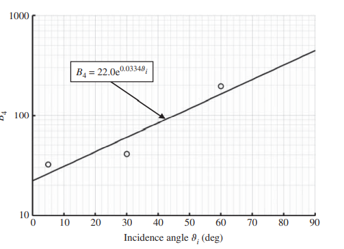
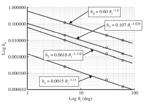
Prokhorov and Prokhorova [3] describe a three-component semiempirical model based on their own measurements of the BRDF of Z302 at a wavelength of $\lambda=10.6 \mu \mathrm{m}$. We have used the same data, represented by the symbols in Figure $4.4$, to derive a purely empirical four-component model, represented by the curves in the figure. Both the Prokhorov and Prokhorova model and our model are in excellent agreement with the measurements. Our four-component model [4] has the form
$$
B R D F=\rho_{1}^{\prime \prime}+\rho_{2}^{\prime \prime}+\rho_{3}^{\prime \prime}+\rho_{4}^{\prime \prime},
$$
where
$$
\rho_{n}^{\prime \prime}=A_{n} \frac{1}{\sqrt{2 \pi} \sigma_{n}} e^{-\left(\vartheta_{v}-\vartheta_{i}\right)^{2} / 2 \sigma_{n}^{2}}+O_{n}, \quad n=1,2,3,4
$$
In Eq. (4.11), $\vartheta_{i}$ and $\vartheta_{v}$ are the incidence and viewing angles shown in the inset in Figure $4.4$, and $A_{n}, \sigma_{n}$, and $O_{n}$ are empirical curve-fitling parameters. The form of Eq. (4.11) is recognizable as the normal probability distribution function multiplied by a scaling factor $A_{n}$ and shifted

in amplitude by an offset $O_{n}$. In practice the additive offsets for the four values of $n$ are gathered into a single constant. The fit illustrated in Figure $4.4$ was obtained by defining the standard deviation
$$
\sigma_{n}=\frac{1}{\sqrt{2 \pi} b_{n} \vartheta_{i}}
$$
and the multiplicative constant
$$
A_{n}=\frac{B_{n}}{b_{n} \vartheta_{i}},
$$

统计代写|蒙特卡洛方法代写Monte Carlo method代考|A Highly Reflective Surface Whose Reflectivity is Strongly Diffuse

We next consider a practical application whose accurate simulation requires a bidirectional spectral reflection model. The integrating sphere [5] often plays a central role in radiometric instrument calibration, surface optical behavior measurement, and radiant source characterization $[6,7]$. The purpose of an integrating sphere is to convert a collimated beam of monochromatic light, such as might be provided by a laser source, into a larger, weaker source of diffuse light at the same wavelength. The essential property of the integrating sphere is its ability to produce a Lambertian source of monochromatic radiation due to multiple scattering from its interior walls. This requirement will be satisfied exactly for a completely enclosed spherical cavity, even when the wall coating is not itself a perfectly diffuse reflector. However, a practical integrating sphere must be fitted with ports that allow the illuminating beam to enter and the instrument under calibration to

view the interior wall. The ports inevitably allow some of the entering radiation to escape before being completely diffused by reflections, thereby compromising the desired effect. In practice the ports are made as small as possible compared to the diameter of the sphere, and the interior walls are treated with a highly reflective, highly diffuse coating.
The author and his coworkers [8] have investigated the departure from ideal behavior of a practical integrating sphere, with emphasis on the influence of directionality. The results of that investigation are offered here as an example of an application in which the diffuse gray assumption may be inadequate. We consider an application in which a relatively small integrating sphere is to be used on-orbit to calibrate a radiometer against a reference radiometer by having both instruments observe the same sector of the interior wall through two separate ports. Because the calibrations will be repeated over a period of up to several years, it is important to know how the calibration factor might be expected to vary with aging of the wall coating. It is further interesting to know how the degree of directionality of reflections from the walls might influence its performance.

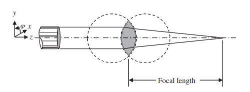
We use the MCRT method to simulate illumination of the interior by a quasi-monochromatic light source at a wavelength, $0.9 \mu \mathrm{m}$, for which the $B R F$ model developed below may be considered valid. For purposes of the current investigation the diameter of the port through which the narrow light beam is admitted may be considered sufficiently small compared to the diameters of the two viewing ports to neglect its presence in the ray trace. The hypothetical experimental arrangement is illustrated in Figure 4.12.

统计代写|蒙特卡洛方法代写Monte Carlo method代考|The Band-Averaged Spectral Radiation

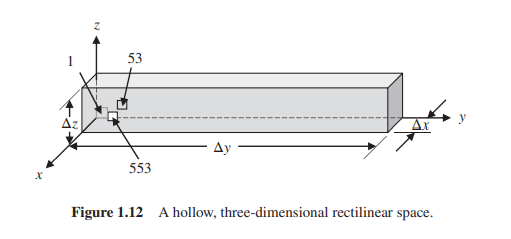
The case studies presented in Sections $4.3$ and $4.4$ exemplify direct application of the MCRT method without recourse to radiation distribution factors, which were not needed to accomplish the stated goals. Furthermore, they involve situations for which the wavelength interval of interest is sufficiently narrow that the surface models used are, to an acceptable approximation, independent of wavelength. However, in some cases radiation distribution factors are required, as explained in Chapter 3. The radiation distribution factor introduced and used in Chapter 3 for gray surfaces had two subscripts, $i$ and $j$, the indices of the emitting and absorbing surface. For the case of spectral radiation it is necessary to add a third subscript, $k$, representing the wavelength interval $\Delta \lambda_{k}$ in which the distribution factor applies. We define the band-averaged spectral radiation distribution factor $D_{i j k}$ as the fraction of power emitted in wavelength

interval $\Delta \lambda_{k}$ by surface element $i$ that is absorbed by surface element $j$, both directly and due to all possible reflections within the enclosure.
Estimation of the band-averaged spectral radiation distribution factor matrix assumes the availability of a dense data set ultimately based on extensive laboratory measurements. Imagine a bookshelf in a virtual thermophysical properties library bearing the label “Bidirectional Spectral Reflectivity.” Upon perusal of this bookshelf we might find books with titles “Z302,” “Spectralon,” “Gold Black,” and other optical coatings. When we take down one of these books and open to its table of contents; we find chapter titles such as “Wavelength Interval Between $0.01$ and $0.10 \mu \mathrm{m}$,” and “Wavelength Interval Between $0.10$ and $1.00 \mu \mathrm{m}$,” and so forth. Then when we flip through Chapter 1 we notice page headings “Angle of Incidence $=5^{\circ}$,” “Angle of Incidence $=10^{\circ}$,” and, on the last page, “Angle of Incidence $=85^{\circ}$.” Finally, when we scan one of these pages from top to bottom we find on the first line “Angle of Reflectance $=5^{\circ}$, $B R D F=44.21$,” and on the second line “Angle of Reflectance $=10^{\circ}$, $B R D F 38.45$,” and so forth. Upon plotting the data found in one of these books, we recognize that the spacing between successive wavelengths, angles of incidence, and angles of reflectance is sufficiently small to allow accurate linear interpolation between tabulated values.

蒙特卡洛方法代考

统计代写|蒙特卡洛方法代写Monte Carlo method代考|A Highly Absorptive Surface Whose Reflectivity is Strongly Specular

气釉®从302[2]是一种基于聚氨酯的涂料，其吸收率通常超过90%在光谱的可见部分，取决于涂层厚度。它的独特之处在于辐射的反射分量大部分是镜面反射的。它的特殊性能使其成为许多航空航天和光学应用的首选涂层，在这些应用中，表面必须是非常有效的吸收体，但不希望出现漫反射。一个典型的应用是用作校准目标的黑体腔的内表面。在这种情况下，腔的几何形状将使得在入射光线能够逸出之前会发生几次镜面反射，并且存在的反射率的任何漫反射分量都会降低设计的有效性，因为它会允许一些功率随着每次反射而逸出腔。这种弥散的“泄漏”可以

当空腔的有效发射率必须是一致的，优于三个九时，这一点非常重要。

Prokhorov 和 Prokhorova [3] 描述了一个三分量半经验模型，该模型基于他们自己对 Z302 在波长为λ=10.6μ米. 我们使用了相同的数据，由图中的符号表示4.4，推导出一个纯经验的四分量模型，由图中的曲线表示。Prokhorov 和 Prokhorova 模型以及我们的模型都与测量结果非常吻合。我们的四分量模型 [4] 具有以下形式

乙RDF=ρ1′′+ρ2′′+ρ3′′+ρ4′′,
在哪里

ρn′′=一个n12圆周率σn和−(ϑ在−ϑ一世)2/2σn2+○n,n=1,2,3,4
在等式。(4.11),ϑ一世和ϑ在是图中插图所示的入射角和视角4.4， 和一个n,σn， 和○n是经验曲线拟合参数。方程的形式。(4.11) 可识别为正态概率分布函数乘以比例因子一个n并转移

幅度偏移○n. 在实践中，四个值的附加偏移量n聚集成一个常数。如图所示的配合4.4通过定义标准偏差获得

σn=12圆周率bnϑ一世
和乘法常数

一个n=乙nbnϑ一世,

统计代写|蒙特卡洛方法代写Monte Carlo method代考|A Highly Reflective Surface Whose Reflectivity is Strongly Diffuse

我们接下来考虑一个实际应用，其精确模拟需要双向光谱反射模型。积分球 [5] 通常在辐射测量仪器校准、表面光学行为测量和辐射源表征中发挥核心作用[6,7]. 积分球的目的是将准直的单色光束（例如可能由激光源提供）转换成更大、更弱的相同波长的漫射光源。积分球的基本特性是由于其内壁的多次散射，它能够产生单色辐射的朗伯源。对于完全封闭的球形空腔，即使壁涂层本身不是完美的漫反射器，该要求也将完全满足。然而，一个实用的积分球必须配备允许照明光束进入的端口，并且被校准的仪器可以

查看内墙。这些端口不可避免地允许一些进入的辐射在被反射完全漫射之前逸出，从而损害所需的效果。实际上，与球体的直径相比，这些端口尽可能地小，并且内壁采用高反射、高漫射涂层处理。
作者和他的同事 [8] 研究了实际积分球与理想行为的偏离，重点是方向性的影响。该调查的结果在此作为一个应用示例提供，其中漫反射灰色假设可能不充分。我们考虑一个应用，其中一个相对较小的积分球将在轨道上用于校准辐射计与参考辐射计，方法是让两个仪器通过两个单独的端口观察内壁的同一扇区。由于校准将在长达数年的时间内重复进行，因此了解校准因子如何随着墙壁涂层的老化而变化非常重要。

我们使用 MCRT 方法来模拟一个波长的准单色光源对内部的照明，0.9μ米, 为此乙RF下面开发的模型可能被认为是有效的。出于当前研究的目的，可以认为窄光束通过的端口的直径与两个观察端口的直径相比足够小，以忽略它在光线轨迹中的存在。假设的实验安排如图 4.12 所示。

统计代写|蒙特卡洛方法代写Monte Carlo method代考|The Band-Averaged Spectral Radiation

章节中介绍的案例研究4.3和4.4举例说明 MCRT 方法的直接应用，无需借助辐射分布因子，而实现既定目标则不需要这些辐射分布因子。此外，它们涉及感兴趣的波长间隔足够窄的情况，以至于所使用的表面模型在可接受的近似值上与波长无关。但是，在某些情况下，需要辐射分布因子，如第 3 章所述。第 3 章介绍和使用的灰色表面的辐射分布因子有两个下标，一世和j，发射和吸收表面的指数。对于光谱辐射的情况，需要添加第三个下标，ķ，代表波长间隔Δλķ其中分布因子适用。我们定义频带平均光谱辐射分布因子D一世jķ作为以波长发射的功率的一部分

间隔Δλķ按面元一世被表面元素吸收j，直接和由于外壳内所有可能的反射。
频带平均光谱辐射分布因子矩阵的估计假设密集数据集的可用性最终基于广泛的实验室测量。想象一下虚拟热物理属性库中的一个书架，上面贴有“双向光谱反射率”标签。仔细阅读这个书架，我们可能会发现标题为“Z302”、“Spectralon”、“Gold Black”和其他光学涂层的书籍。当我们取下其中一本书并打开其目录时；我们找到章节标题，例如“Wavelength Interval Between0.01和0.10μ米,”和“波长间隔0.10和1.00μ米,”等等。然后，当我们翻阅第 1 章时，我们注意到页面标题“入射角=5∘，“ “入射角=10∘,”以及最后一页的“入射角=85∘。” 最后，当我们从上到下扫描其中一个页面时，我们在第一行发现“反射角=5∘, 乙RDF=44.21,”和第二行的“反射角=10∘,乙RDF38.45,”等等。在绘制其中一本书中的数据后，我们认识到连续波长、入射角和反射角之间的间距足够小，可以在表格值之间进行准确的线性插值。

统计代写请认准statistics-lab™. statistics-lab™为您的留学生涯保驾护航。

金融工程代写

金融工程是使用数学技术来解决金融问题。金融工程使用计算机科学、统计学、经济学和应用数学领域的工具和知识来解决当前的金融问题，以及设计新的和创新的金融产品。

非参数统计代写

非参数统计指的是一种统计方法，其中不假设数据来自于由少数参数决定的规定模型；这种模型的例子包括正态分布模型和线性回归模型。

广义线性模型代考

广义线性模型（GLM）归属统计学领域，是一种应用灵活的线性回归模型。该模型允许因变量的偏差分布有除了正态分布之外的其它分布。

术语 广义线性模型（GLM）通常是指给定连续和/或分类预测因素的连续响应变量的常规线性回归模型。它包括多元线性回归，以及方差分析和方差分析（仅含固定效应）。

有限元方法代写

有限元方法（FEM）是一种流行的方法，用于数值解决工程和数学建模中出现的微分方程。典型的问题领域包括结构分析、传热、流体流动、质量运输和电磁势等传统领域。

有限元是一种通用的数值方法，用于解决两个或三个空间变量的偏微分方程（即一些边界值问题）。为了解决一个问题，有限元将一个大系统细分为更小、更简单的部分，称为有限元。这是通过在空间维度上的特定空间离散化来实现的，它是通过构建对象的网格来实现的：用于求解的数值域，它有有限数量的点。边界值问题的有限元方法表述最终导致一个代数方程组。该方法在域上对未知函数进行逼近。[1] 然后将模拟这些有限元的简单方程组合成一个更大的方程系统，以模拟整个问题。然后，有限元通过变化微积分使相关的误差函数最小化来逼近一个解决方案。

tatistics-lab作为专业的留学生服务机构，多年来已为美国、英国、加拿大、澳洲等留学热门地的学生提供专业的学术服务，包括但不限于Essay代写，Assignment代写，Dissertation代写，Report代写，小组作业代写，Proposal代写，Paper代写，Presentation代写，计算机作业代写，论文修改和润色，网课代做，exam代考等等。写作范围涵盖高中，本科，研究生等海外留学全阶段，辐射金融，经济学，会计学，审计学，管理学等全球99%专业科目。写作团队既有专业英语母语作者，也有海外名校硕博留学生，每位写作老师都拥有过硬的语言能力，专业的学科背景和学术写作经验。我们承诺100%原创，100%专业，100%准时，100%满意。

随机分析代写

随机微积分是数学的一个分支，对随机过程进行操作。它允许为随机过程的积分定义一个关于随机过程的一致的积分理论。这个领域是由日本数学家伊藤清在第二次世界大战期间创建并开始的。

时间序列分析代写

随机过程，是依赖于参数的一组随机变量的全体，参数通常是时间。 随机变量是随机现象的数量表现，其时间序列是一组按照时间发生先后顺序进行排列的数据点序列。通常一组时间序列的时间间隔为一恒定值（如1秒，5分钟，12小时，7天，1年），因此时间序列可以作为离散时间数据进行分析处理。研究时间序列数据的意义在于现实中，往往需要研究某个事物其随时间发展变化的规律。这就需要通过研究该事物过去发展的历史记录，以得到其自身发展的规律。

回归分析代写

多元回归分析渐进（Multiple Regression Analysis Asymptotics）属于计量经济学领域，主要是一种数学上的统计分析方法，可以分析复杂情况下各影响因素的数学关系，在自然科学、社会和经济学等多个领域内应用广泛。

MATLAB代写

MATLAB 是一种用于技术计算的高性能语言。它将计算、可视化和编程集成在一个易于使用的环境中，其中问题和解决方案以熟悉的数学符号表示。典型用途包括：数学和计算算法开发建模、仿真和原型制作数据分析、探索和可视化科学和工程图形应用程序开发，包括图形用户界面构建MATLAB 是一个交互式系统，其基本数据元素是一个不需要维度的数组。这使您可以解决许多技术计算问题，尤其是那些具有矩阵和向量公式的问题，而只需用 C 或 Fortran 等标量非交互式语言编写程序所需的时间的一小部分。MATLAB 名称代表矩阵实验室。MATLAB 最初的编写目的是提供对由 LINPACK 和 EISPACK 项目开发的矩阵软件的轻松访问，这两个项目共同代表了矩阵计算软件的最新技术。MATLAB 经过多年的发展，得到了许多用户的投入。在大学环境中，它是数学、工程和科学入门和高级课程的标准教学工具。在工业领域，MATLAB 是高效研究、开发和分析的首选工具。MATLAB 具有一系列称为工具箱的特定于应用程序的解决方案。对于大多数 MATLAB 用户来说非常重要，工具箱允许您学习和应用专业技术。工具箱是 MATLAB 函数（M 文件）的综合集合，可扩展 MATLAB 环境以解决特定类别的问题。可用工具箱的领域包括信号处理、控制系统、神经网络、模糊逻辑、小波、仿真等。

R语言代写	问卷设计与分析代写
PYTHON代写	回归分析与线性模型代写
MATLAB代写	方差分析与试验设计代写
STATA代写	机器学习/统计学习代写
SPSS代写	计量经济学代写
EVIEWS代写	时间序列分析代写
EXCEL代写	深度学习代写
SQL代写	各种数据建模与可视化代写

如果你也在 怎样代写蒙特卡洛方法Monte Carlo method这个学科遇到相关的难题，请随时右上角联系我们的24/7代写客服。

蒙特卡洛方法，或称蒙特卡洛实验，是一类广泛的计算算法，依靠重复随机抽样来获得数值结果。其基本概念是利用随机性来解决原则上可能是确定性的问题。

statistics-lab™ 为您的留学生涯保驾护航 在代写蒙特卡洛方法Monte Carlo method方面已经树立了自己的口碑, 保证靠谱, 高质且原创的统计Statistics代写服务。我们的专家在代写蒙特卡洛方法Monte Carlo method代写方面经验极为丰富，各种代写蒙特卡洛方法Monte Carlo method相关的作业也就用不着说。

我们提供的蒙特卡洛方法Monte Carlo method及其相关学科的代写，服务范围广, 其中包括但不限于:

• Statistical Inference 统计推断
• Statistical Computing 统计计算
• Advanced Probability Theory 高等概率论
• Advanced Mathematical Statistics 高等数理统计学
• (Generalized) Linear Models 广义线性模型
• Statistical Machine Learning 统计机器学习
• Longitudinal Data Analysis 纵向数据分析
• Foundations of Data Science 数据科学基础

统计代写|蒙特卡洛方法代写Monte Carlo method代考|Use of Radiation Distribution Factors When Some Surface Net Heat Fluxes Are Specified

We now address the situation where surface elements $1,2, \ldots, N$ have specified net heat fluxes and surfaces $N+1, N+2, \ldots, n$ have specified temperatures. To begin, let us consider the special case where $N=1$; that is, where only the first of $n$ surface elements has a specified net heat flux, with the remaining surfaces having specified temperatures. In this case Eq. (3.35) may be written
$$
q_{1}=\varepsilon_{1}\left[\left(1-D_{11}\right) \sigma T_{1}^{4}-\sum_{j=2}^{n} \sigma T_{j}^{4} D_{i j}\right]
$$
Equation (3.36) can be solved explicitly for the unknown surface temperature $T_{1}$ in terms of the known surface net heat flux $q_{1}$ and the known surface temperatures; that is,
$$
\sigma T_{1}^{4}=\frac{1}{1-D_{11}}\left(\frac{q_{1}}{\varepsilon_{1}}+\sum_{j=2}^{n} \sigma T_{j}^{4} D_{i j}\right)
$$
In the more general case where several surface elements have specified net heat fluxes we can rearrange Eq. (3.35) to obtain
$$
q_{i}+\varepsilon_{i} \sum_{j=N+1}^{n} \sigma T_{j}^{4} D_{i j}=\varepsilon_{i} \sum_{j=1}^{N} \sigma T_{j}^{4}\left(\delta_{i j}-D_{i j}\right), \quad 1 \leq i \leq N_{\star}
$$

Equation (3.38) represents $N$ equations in the $N$ unknown surface temperatures in terms of the $N$ known surface net heat fluxes and the $n-N$ known surface temperatures. It can be rewritten symbolically as
$$
\Theta_{i}=\Psi_{i j} \Omega_{j},
$$
where
$$
\Theta_{i}=q_{i}+\varepsilon_{i} \sum_{j=N+1}^{n} \sigma T_{j}^{4} D_{i j}, \quad 1 \leq i \leq N,
$$
is a known vector,
$$
\Psi_{i j}=\varepsilon_{i}\left(\delta_{i j}-D_{i j}\right), \quad 1 \leq i \leq N, \quad 1 \leq j \leq N,
$$
and
$$
\Omega_{j}=\sigma T_{j}^{4}, \quad 1 \leq j \leq N,
$$
is an unknown vector whose elements are sought. We obtain the unknown surface temperatures by inverting the matrix defined by Eq. (3.41) and then using it to operate on the vector defined by Eq. (3.40); that is,
$$
\Omega_{i}=\left[\Psi_{i j}\right]^{-1} \Theta_{j}, \quad 1 \leq i \leq N .
$$
The unknown surface net heat fluxes are then computed using Eq. (3.35) applied over the range $N+1 \leq i \leq n$.

统计代写|蒙特卡洛方法代写Monte Carlo method代考|Bidirectional Spectral Surfaces

Experience confirms that reflection from a surface is generally neither diffuse nor specular. Rather, at a given wavelength the distribution of reflected energy depends on the mechanical and chemical preparation

of the surface and on the direction of incidence. Diffuse and specular reflections represent the two extremes of bidirectional reflectivity. Both extremes may be approached but rarely achieved in practice. Various theories have been proposed for predicting bidirectional spectral reflection and directional spectral emission and absorption for generic surfaces. The interested reader is referred to Chapter 4 in Ref. [1], where this topic is pursued in more detail. However, metrology remains the only sure path to surface models that accurately capture the directional spectral behavior of real surfaces.

A simple two-component model for directional reflectivity was introduced in Chapter 1 (Figure 1.9), where it is suggested that a directional reflection pattern can be somewhat approximated as a suitably weighted combination of spectral and diffuse reflection. Different versions of this approximation would have to be applied for each wavelength of interest, using different weight factors for each wavelength. Any success this approach might have would be due in large measure to the fact that the distribution of radiant energy within an enclosure is governed by integral equations rather than by differential equations. Integration at least partially “averages out” positive and negative excursions from reality, as illustrated in Figure 4.1. Inspection of the figure reveals that, even though

$f_{1}(x)$ is a more detailed and presumably more accurate description of local behavior than $f_{2}(x)$, it may nonetheless be true, to an acceptable approximation, that
$$
\int_{0}^{1} f_{1}(x) d x \cong \int_{0}^{1} f_{2}(x) d x
$$

统计代写|蒙特卡洛方法代写Monte Carlo method代考|Principles Underlying a Practical Bidirectional Reflection Model

Useful bidirectional reflection models are generally based on measurements, although they are frequently informed by theory. As we learned in Sections $2.12$ and $2.13$, the optical behaviors of electrically non-conducting (dielectric) and electrically conducting (metal) surfaces are fundamentally different. In general, metal surfaces are strong specular reflectors while dielectric surfaces tend to be weak diffuse reflectors. In both cases the directional distribution of reflected radiation is known to be strongly influenced by the topography, chemical state, and degree of contamination of the surface. With the exception of certain optical components (such as mirrors, lenses, and filters), it is unlikely that a bidirectional spectral reflectivity model based entirely on theory would accurately represent the optical behavior of a surface of practical engineering interest. Therefore, in cases where high accuracy is required, a successful surface optical model must be at least semiempirical if not based entirely on measurements of the optical behavior of the surface to be modeled.

In this chapter we first demonstrate the application of semiempirical approaches for two surface coatings engineered to exhibit specific $-$ and somewhat unique – optical behaviors. In the first example we consider a highly absorptive commercial coating whose small component of reflectivity is highly directional to the point of being almost specular, and in the second example we consider another commercial coating that is highly reflective but whose reflectivity is nearly diffuse. Both of these coatings are widely used in optical applications requiring an unusual combination of both metallic and dielectric behaviors. We then follow up by presenting a completely general approach suitable for applications where a full set of experimental data is available.

We begin by recalling the bidirectional spectral reflectivity from Chapter 2,$\begin{aligned} \rho_{\lambda}^{\prime \prime} &=\rho\left(\lambda, \vartheta_{i}, \varphi_{i}, \vartheta_{r}, \varphi_{r}\right) \equiv \frac{d i_{\lambda, r}\left(\lambda, \vartheta_{i}, \varphi_{i}, \vartheta_{r}, \varphi_{r}\right)}{i_{\lambda, i}\left(\lambda, \vartheta_{i}, \varphi_{i}\right) \cos \vartheta_{i} d \Omega_{i}} \ & \equiv B R D F\left(\lambda, \vartheta_{i}, \varphi_{i}, \vartheta_{r}, \varphi_{r}\right) \end{aligned}$

蒙特卡洛方法代考

统计代写|蒙特卡洛方法代写Monte Carlo method代考|Use of Radiation Distribution Factors When Some Surface Net Heat Fluxes Are Specified

我们现在解决表面元素的情况1,2,…,ñ具有指定的净热通量和表面ñ+1,ñ+2,…,n有规定的温度。首先，让我们考虑一下特殊情况ñ=1; 也就是说，只有第一个n表面元素具有指定的净热通量，其余表面具有指定的温度。在这种情况下，方程式。(3.35) 可以写成

q1=e1[(1−D11)σ吨14−∑j=2nσ吨j4D一世j]
对于未知的表面温度，方程 (3.36) 可以明确求解吨1根据已知的表面净热通量q1和已知的表面温度；那是，

σ吨14=11−D11(q1e1+∑j=2nσ吨j4D一世j)
在更一般的情况下，几个表面元素指定了净热通量，我们可以重新排列方程。(3.35) 获得

q一世+e一世∑j=ñ+1nσ吨j4D一世j=e一世∑j=1ñσ吨j4(d一世j−D一世j),1≤一世≤ñ⋆

等式 (3.38) 表示ñ中的方程ñ未知的表面温度ñ已知地表净热通量和n−ñ已知的表面温度。它可以象征性地重写为

θ一世=Ψ一世jΩj,
在哪里

θ一世=q一世+e一世∑j=ñ+1nσ吨j4D一世j,1≤一世≤ñ,
是一个已知向量，

Ψ一世j=e一世(d一世j−D一世j),1≤一世≤ñ,1≤j≤ñ,
和

Ωj=σ吨j4,1≤j≤ñ,
是寻找其元素的未知向量。我们通过反转方程式定义的矩阵来获得未知的表面温度。（3.41）然后用它对方程定义的向量进行操作。（3.40）；那是，

Ω一世=[Ψ一世j]−1θj,1≤一世≤ñ.
然后使用方程式计算未知的表面净热通量。(3.35) 应用于范围ñ+1≤一世≤n.

统计代写|蒙特卡洛方法代写Monte Carlo method代考|Bidirectional Spectral Surfaces

经验证实，来自表面的反射通常既不是漫反射也不是镜面反射。相反，在给定波长下，反射能量的分布取决于机械和化学制备

表面和入射方向。漫反射和镜面反射代表双向反射率的两个极端。这两个极端都可以接近，但在实践中很少能实现。已经提出了各种理论来预测通用表面的双向光谱反射和定向光谱发射和吸收。感兴趣的读者可以参考参考文献中的第 4 章。[1]，其中更详细地探讨了该主题。然而，计量学仍然是获得准确捕捉真实表面的定向光谱行为的表面模型的唯一可靠途径。

第 1 章介绍了一个简单的定向反射率双分量模型（图 1.9），其中建议定向反射模式在某种程度上可以近似为光谱和漫反射的适当加权组合。这种近似的不同版本必须应用于每个感兴趣的波长，对每个波长使用不同的权重因子。这种方法可能取得的任何成功在很大程度上归功于这样一个事实，即外壳内的辐射能分布由积分方程而不是微分方程控制。如图 4.1 所示，整合至少部分地“平均”了现实中的正负偏移。对该图的检查表明，即使

F1(X)是对局部行为的更详细和可能更准确的描述F2(X)，但在可接受的近似值上，它可能是正确的，即

∫01F1(X)dX≅∫01F2(X)dX

统计代写|蒙特卡洛方法代写Monte Carlo method代考|Principles Underlying a Practical Bidirectional Reflection Model

有用的双向反射模型通常基于测量值，尽管它们经常受到理论的影响。正如我们在章节中学到的2.12和2.13，不导电（电介质）和导电（金属）表面的光学行为根本不同。一般来说，金属表面是强镜面反射器，而电介质表面往往是弱漫反射器。在这两种情况下，反射辐射的方向分布都受到表面的地形、化学状态和污染程度的强烈影响。除了某些光学组件（例如镜子、透镜和滤光片）之外，完全基于理论的双向光谱反射率模型不太可能准确地表示具有实际工程兴趣的表面的光学行为。因此，在需要高精度的情况下，

在本章中，我们首先展示了半经验方法对两种表面涂层的应用，这些涂层被设计为展示特定的−并且有些独特 – 光学行为。在第一个示例中，我们考虑了一种高吸收性商业涂层，其反射率的小部分高度定向到几乎是镜面的点，在第二个示例中，我们考虑了另一种高反射率但反射率几乎是漫射的商业涂层。这两种涂层都广泛用于需要金属和介电行为的不寻常组合的光学应用。然后，我们提出了一种完全通用的方法，适用于有全套实验数据的应用程序。

我们首先回顾第 2 章中的双向光谱反射率，ρλ′′=ρ(λ,ϑ一世,披一世,ϑr,披r)≡d一世λ,r(λ,ϑ一世,披一世,ϑr,披r)一世λ,一世(λ,ϑ一世,披一世)因⁡ϑ一世dΩ一世 ≡乙RDF(λ,ϑ一世,披一世,ϑr,披r)

统计代写请认准statistics-lab™. statistics-lab™为您的留学生涯保驾护航。

金融工程代写

金融工程是使用数学技术来解决金融问题。金融工程使用计算机科学、统计学、经济学和应用数学领域的工具和知识来解决当前的金融问题，以及设计新的和创新的金融产品。

非参数统计代写

非参数统计指的是一种统计方法，其中不假设数据来自于由少数参数决定的规定模型；这种模型的例子包括正态分布模型和线性回归模型。

广义线性模型代考

广义线性模型（GLM）归属统计学领域，是一种应用灵活的线性回归模型。该模型允许因变量的偏差分布有除了正态分布之外的其它分布。

术语 广义线性模型（GLM）通常是指给定连续和/或分类预测因素的连续响应变量的常规线性回归模型。它包括多元线性回归，以及方差分析和方差分析（仅含固定效应）。

有限元方法代写

有限元方法（FEM）是一种流行的方法，用于数值解决工程和数学建模中出现的微分方程。典型的问题领域包括结构分析、传热、流体流动、质量运输和电磁势等传统领域。

有限元是一种通用的数值方法，用于解决两个或三个空间变量的偏微分方程（即一些边界值问题）。为了解决一个问题，有限元将一个大系统细分为更小、更简单的部分，称为有限元。这是通过在空间维度上的特定空间离散化来实现的，它是通过构建对象的网格来实现的：用于求解的数值域，它有有限数量的点。边界值问题的有限元方法表述最终导致一个代数方程组。该方法在域上对未知函数进行逼近。[1] 然后将模拟这些有限元的简单方程组合成一个更大的方程系统，以模拟整个问题。然后，有限元通过变化微积分使相关的误差函数最小化来逼近一个解决方案。

tatistics-lab作为专业的留学生服务机构，多年来已为美国、英国、加拿大、澳洲等留学热门地的学生提供专业的学术服务，包括但不限于Essay代写，Assignment代写，Dissertation代写，Report代写，小组作业代写，Proposal代写，Paper代写，Presentation代写，计算机作业代写，论文修改和润色，网课代做，exam代考等等。写作范围涵盖高中，本科，研究生等海外留学全阶段，辐射金融，经济学，会计学，审计学，管理学等全球99%专业科目。写作团队既有专业英语母语作者，也有海外名校硕博留学生，每位写作老师都拥有过硬的语言能力，专业的学科背景和学术写作经验。我们承诺100%原创，100%专业，100%准时，100%满意。

随机分析代写

随机微积分是数学的一个分支，对随机过程进行操作。它允许为随机过程的积分定义一个关于随机过程的一致的积分理论。这个领域是由日本数学家伊藤清在第二次世界大战期间创建并开始的。

时间序列分析代写

随机过程，是依赖于参数的一组随机变量的全体，参数通常是时间。 随机变量是随机现象的数量表现，其时间序列是一组按照时间发生先后顺序进行排列的数据点序列。通常一组时间序列的时间间隔为一恒定值（如1秒，5分钟，12小时，7天，1年），因此时间序列可以作为离散时间数据进行分析处理。研究时间序列数据的意义在于现实中，往往需要研究某个事物其随时间发展变化的规律。这就需要通过研究该事物过去发展的历史记录，以得到其自身发展的规律。

回归分析代写

多元回归分析渐进（Multiple Regression Analysis Asymptotics）属于计量经济学领域，主要是一种数学上的统计分析方法，可以分析复杂情况下各影响因素的数学关系，在自然科学、社会和经济学等多个领域内应用广泛。

MATLAB代写

MATLAB 是一种用于技术计算的高性能语言。它将计算、可视化和编程集成在一个易于使用的环境中，其中问题和解决方案以熟悉的数学符号表示。典型用途包括：数学和计算算法开发建模、仿真和原型制作数据分析、探索和可视化科学和工程图形应用程序开发，包括图形用户界面构建MATLAB 是一个交互式系统，其基本数据元素是一个不需要维度的数组。这使您可以解决许多技术计算问题，尤其是那些具有矩阵和向量公式的问题，而只需用 C 或 Fortran 等标量非交互式语言编写程序所需的时间的一小部分。MATLAB 名称代表矩阵实验室。MATLAB 最初的编写目的是提供对由 LINPACK 和 EISPACK 项目开发的矩阵软件的轻松访问，这两个项目共同代表了矩阵计算软件的最新技术。MATLAB 经过多年的发展，得到了许多用户的投入。在大学环境中，它是数学、工程和科学入门和高级课程的标准教学工具。在工业领域，MATLAB 是高效研究、开发和分析的首选工具。MATLAB 具有一系列称为工具箱的特定于应用程序的解决方案。对于大多数 MATLAB 用户来说非常重要，工具箱允许您学习和应用专业技术。工具箱是 MATLAB 函数（M 文件）的综合集合，可扩展 MATLAB 环境以解决特定类别的问题。可用工具箱的领域包括信号处理、控制系统、神经网络、模糊逻辑、小波、仿真等。

R语言代写	问卷设计与分析代写
PYTHON代写	回归分析与线性模型代写
MATLAB代写	方差分析与试验设计代写
STATA代写	机器学习/统计学习代写
SPSS代写	计量经济学代写
EVIEWS代写	时间序列分析代写
EXCEL代写	深度学习代写
SQL代写	各种数据建模与可视化代写

如果你也在 怎样代写蒙特卡洛方法Monte Carlo method这个学科遇到相关的难题，请随时右上角联系我们的24/7代写客服。

蒙特卡洛方法，或称蒙特卡洛实验，是一类广泛的计算算法，依靠重复随机抽样来获得数值结果。其基本概念是利用随机性来解决原则上可能是确定性的问题。

statistics-lab™ 为您的留学生涯保驾护航 在代写蒙特卡洛方法Monte Carlo method方面已经树立了自己的口碑, 保证靠谱, 高质且原创的统计Statistics代写服务。我们的专家在代写蒙特卡洛方法Monte Carlo method代写方面经验极为丰富，各种代写蒙特卡洛方法Monte Carlo method相关的作业也就用不着说。

我们提供的蒙特卡洛方法Monte Carlo method及其相关学科的代写，服务范围广, 其中包括但不限于:

• Statistical Inference 统计推断
• Statistical Computing 统计计算
• Advanced Probability Theory 高等概率论
• Advanced Mathematical Statistics 高等数理统计学
• (Generalized) Linear Models 广义线性模型
• Statistical Machine Learning 统计机器学习
• Longitudinal Data Analysis 纵向数据分析
• Foundations of Data Science 数据科学基础

统计代写|蒙特卡洛方法代写Monte Carlo method代考|Binning of Rays on a Surface Element; Illustrative Example

Meshing and indexing are treated in Section 1.6. A closely related idea is binning, in which indexing allows us to keep track of the spatial distribution of absorbed energy bundles. In the case of the instrument in Figure 3.2, it might be desirable to know how the power incident to the entrance aperture is distributed across the detector face. In this situation, after executing Step 11, control is transferred to a binning step not shown in Figure 3.1. The detector surface, subdivided into a number of bins, is illustrated in Figure 3.5. In a given application the actual number of bins and their spatial distribution would be dictated by the shape of the surface and the desired spatial resolution.

No attempt has been made in creating Figure $3.5$ to suggest a particular scheme for determining the spacing between consecutive radial rings. However, two schemes come to mind: (i) either the ring boundaries could be equally spaced or (ii) they could be spaced to achieve equal-area rings. The former scheme is, of course, easy to achieve but is probably

not as useful as the latter. A plot of power absorbed as a function of radial position would be easier to interpret if the rings were divided into equal areas. This may be achieved using the formula
$$
r_{m}=(d / 2) \sqrt{m / M}
$$
where $d$ is the diameter of the detector, $M$ is the total number of radial bands to be created, and $r_{m}$ is the radial position of the outer radius of the $m$ th band. It is both natural and convenient to base the circumferential divisions on equal angles,
$$
\varphi_{n}=2 \pi n / N,
$$
where $N$ is the total number of angular sectors, $n$ is the $n$th such sector, and $\varphi_{n}$ is the angle corresponding to the upper angular limit of the sector.

We arrive at the binning step with knowledge of $x_{1}, y_{1}, z_{1}$, and $P_{1}$, where $P_{1}$ is the power carried by the current ray. The Matlab function for determining the values of $m$ and $n$ and updating the power accumulated in bin $(m, n)$ appears in Figure 3.6. The “floor” operator on lines 8 and 12 of Figure $3.6$ returns the least integer in the argument.

统计代写|蒙特卡洛方法代写Monte Carlo method代考|Thermal and Optical Analysis

Figure $3.7$ is a detailed data sheet for the radiometric instrument concept illustrated in Figure 3.2. Our task is to provide a preliminary evaluation of its optical and thermal performance. The approach is to model the

optical behavior of the instrument under the assumption of specularly reflecting mirrors and diffuse-specular non-mirror surfaces in the visible wavelength range $(0.4-0.7 \mu \mathrm{m})$, and to model the thermal behavior of the instrument in the infrared. Optical characterization will require assessment of baffle and telescope performance, while thermal characterization will require estimation of the distribution factor matrix. The listing for the Matlab code developed to accomplish this task is available at the companion website listed on p. xix. Study of the code listing reveals that the component geometries and dimensions have been entered “by hand.” However, it is possible to import system geometries directly into Matlab from the CAD environment where they were created.

The first step is to determine the distance from the entrance aperture to the focal plane. This task is accomplished by performing a numerical experiment in which an on-axis collimated beam consisting of 100000 rays is introduced through the instrument aperture. The detector is then displaced back and forth along the optical axis until the waist diameter of the twice-reflected beam is minimized. The result of this process, obtained by iteration, is shown in Figure 3.8, in which the rays have converged to a circle of minimum diameter at $z=58.5823 \mathrm{~mm}$. The notation “TBD” in Figure $3.7$ can now be replaced with this value, and the preliminary design of the instrument is complete.

In Figures $3.9$ and 3.10, the intersections of rays with the primary and secondary mirrors are shown as individual dots. These and similar plots for the other surfaces of the instrument are invaluable for confirming the basic design assumptions, such as symmetry in this example.

统计代写|蒙特卡洛方法代写Monte Carlo method代考|Use of Radiation Distribution Factors for the Case of Specified Surface Temperatures

Consider the special case where all of the surface elements making up the generic enclosure shown schematically in Figure $3.17$ have specified temperatures, and where all of the surface net heat fluxes are unknown. Note that the view of some surface elements may be either partially or fully blocked when viewed from other surface elements. This does not present a problem in the following analysis because partial or full blockage of direct radiation has already been accounted for in the definition and estimation of the distribution factors, as has the effect of surface curvature.

Consistent with the definition of the diffuse-specular graybody radiation distribution factor, we can express the radiation heat flux $\left(\mathrm{W} \mathrm{m}^{-2}\right.$ )

absorbed by surface element $i$ due to emission from all of the surface elements making up the enclosure
$$
q_{i, a}=\frac{Q_{i, a}}{A_{i}}=\frac{1}{A_{i}} \sum_{j=1}^{n} \varepsilon_{j} A_{j} \sigma T_{j}^{4} D_{j i}, \quad 1 \leq i \leq n,
$$
which, with the introduction of reciprocity, Eq. (3.5), becomes
$$
q_{i, a}=\varepsilon_{i} \sum_{j=1}^{n} \sigma T_{j}^{4} D_{i j} . \quad 1 \leq i \leq n .
$$
The radiation heat flux emitted from surface element $i$ is
$$
q_{i, e}=\frac{Q_{i, e}}{A_{i}}=\frac{\varepsilon_{i} A_{i} \sigma T_{i}^{4}}{A_{i}}=\varepsilon_{i} \sigma T_{i}^{4}, \quad 1 \leq i \leq n
$$
Then the net heat flux from surface element $i$ is
$$
q_{i}=q_{i, e}-q_{i, a}=\varepsilon_{i} \sigma T_{i}^{4}-\varepsilon_{i} \sum_{j=1}^{n} \sigma T_{j}^{4} D_{i j}, \quad 1 \leq i \leq n
$$
or, with the introduction of the Kronecker delta
$$
\delta_{i j} \equiv \begin{cases}1, & i=j \ 0, & i \neq j\end{cases}
$$
Eq. (3.33) can be written
$$
q_{i}=\varepsilon_{i} \sum_{j=1}^{n} \sigma T_{j}^{4}\left(\delta_{i j}-D_{i j}\right) \quad 1 \leq i \leq n
$$

蒙特卡洛方法代考

统计代写|蒙特卡洛方法代写Monte Carlo method代考|Binning of Rays on a Surface Element; Illustrative Example

网格化和索引在 1.6 节中讨论。一个密切相关的想法是分箱，其中索引允许我们跟踪吸收的能量束的空间分布。对于图 3.2 中的仪器，可能需要知道入射到入口孔径的功率如何在探测器表面上分布。在这种情况下，执行步骤 11 后，控制转移到图 3.1 中未显示的分箱步骤。检测器表面被细分为多个 bin，如图 3.5 所示。在给定的应用中，实际的 bin 数量及其空间分布将由表面的形状和所需的空间分辨率决定。

没有尝试创建Figure3.5建议确定连续径向环之间间距的特定方案。然而，我想到了两种方案：（i）环边界可以等间距或（ii）它们可以隔开以实现等面积的环。前一种方案当然很容易实现，但可能

不如后者有用。如果将环分成相等的区域，则作为径向位置函数的吸收功率图将更容易解释。这可以使用公式来实现

r米=(d/2)米/米
在哪里d是探测器的直径，米是要创建的径向带的总数，并且r米是外半径的径向位置米乐队。以等角为基础的圆周划分既自然又方便，

披n=2圆周率n/ñ,
在哪里ñ是角扇区的总数，n是个n此类部门，以及披n是对应于扇区角上限的角度。

我们到达装箱步骤时知道X1,是1,和1， 和磷1， 在哪里磷1是当前射线携带的能量。用于确定值的 Matlab 函数米和n并更新 bin 中累积的功率(米,n)如图 3.6 所示。图的第 8 行和第 12 行的“floor”运算符3.6返回参数中的最小整数。

统计代写|蒙特卡洛方法代写Monte Carlo method代考|Thermal and Optical Analysis

数字3.7是图 3.2 中所示的辐射测量仪器概念的详细数据表。我们的任务是对其光学和热性能进行初步评估。方法是建模

假设镜面反射镜和漫反射非镜面在可见波长范围内的仪器光学行为(0.4−0.7μ米)，并模拟仪器在红外线中的热行为。光学特性需要评估挡板和望远镜的性能，而热特性需要估计分布因子矩阵。为完成此任务而开发的 Matlab 代码清单可在第 4 页列出的配套网站上找到。十九。对代码清单的研究表明，组件的几何形状和尺寸是“手工”输入的。但是，可以将系统几何图形从创建它们的 CAD 环境直接导入 Matlab。

第一步是确定从入口孔径到焦平面的距离。这项任务是通过进行数值实验来完成的，在该实验中，由 100000 条光线组成的轴上准直光束通过仪器孔径引入。然后检测器沿光轴来回移动，直到两次反射光束的腰部直径最小。这个过程通过迭代得到的结果如图 3.8 所示，其中光线在和=58.5823 米米. 图中的符号“TBD”3.7现在可以用这个值代替，仪器的初步设计就完成了。

在数字3.9在图 3.10 和 3.10 中，光线与主镜和次镜的交点显示为单独的点。仪器其他表面的这些和类似图对于确认基本设计假设（例如本例中的对称性）非常宝贵。

统计代写|蒙特卡洛方法代写Monte Carlo method代考|Use of Radiation Distribution Factors for the Case of Specified Surface Temperatures

考虑一种特殊情况，其中所有表面元素构成图 1 中示意性地显示的通用外壳。3.17具有指定的温度，并且所有表面净热通量都是未知的。请注意，当从其他表面元素查看时，某些表面元素的视图可能会部分或完全被遮挡。这在下面的分析中不会出现问题，因为在分布因子的定义和估计中已经考虑了直接辐射的部分或完全阻挡，表面曲率的影响也是如此。

与漫反射灰体辐射分布因子的定义一致，可以表示辐射热通量(在米−2 )

被表面元素吸收一世由于构成外壳的所有表面元素的发射

q一世,一个=问一世,一个一个一世=1一个一世∑j=1nej一个jσ吨j4Dj一世,1≤一世≤n,
其中，随着互惠的引入，方程式。(3.5)，变为

q一世,一个=e一世∑j=1nσ吨j4D一世j.1≤一世≤n.
面元发出的辐射热通量一世是

q一世,和=问一世,和一个一世=e一世一个一世σ吨一世4一个一世=e一世σ吨一世4,1≤一世≤n
然后是来自表面元素的净热通量一世是

q一世=q一世,和−q一世,一个=e一世σ吨一世4−e一世∑j=1nσ吨j4D一世j,1≤一世≤n
或者，随着克罗内克三角洲的引入

d一世j≡{1,一世=j 0,一世≠j
方程。(3.33) 可以写成

q一世=e一世∑j=1nσ吨j4(d一世j−D一世j)1≤一世≤n

统计代写请认准statistics-lab™. statistics-lab™为您的留学生涯保驾护航。

金融工程代写

金融工程是使用数学技术来解决金融问题。金融工程使用计算机科学、统计学、经济学和应用数学领域的工具和知识来解决当前的金融问题，以及设计新的和创新的金融产品。

非参数统计代写

非参数统计指的是一种统计方法，其中不假设数据来自于由少数参数决定的规定模型；这种模型的例子包括正态分布模型和线性回归模型。

广义线性模型代考

广义线性模型（GLM）归属统计学领域，是一种应用灵活的线性回归模型。该模型允许因变量的偏差分布有除了正态分布之外的其它分布。

术语 广义线性模型（GLM）通常是指给定连续和/或分类预测因素的连续响应变量的常规线性回归模型。它包括多元线性回归，以及方差分析和方差分析（仅含固定效应）。

有限元方法代写

有限元方法（FEM）是一种流行的方法，用于数值解决工程和数学建模中出现的微分方程。典型的问题领域包括结构分析、传热、流体流动、质量运输和电磁势等传统领域。

有限元是一种通用的数值方法，用于解决两个或三个空间变量的偏微分方程（即一些边界值问题）。为了解决一个问题，有限元将一个大系统细分为更小、更简单的部分，称为有限元。这是通过在空间维度上的特定空间离散化来实现的，它是通过构建对象的网格来实现的：用于求解的数值域，它有有限数量的点。边界值问题的有限元方法表述最终导致一个代数方程组。该方法在域上对未知函数进行逼近。[1] 然后将模拟这些有限元的简单方程组合成一个更大的方程系统，以模拟整个问题。然后，有限元通过变化微积分使相关的误差函数最小化来逼近一个解决方案。

tatistics-lab作为专业的留学生服务机构，多年来已为美国、英国、加拿大、澳洲等留学热门地的学生提供专业的学术服务，包括但不限于Essay代写，Assignment代写，Dissertation代写，Report代写，小组作业代写，Proposal代写，Paper代写，Presentation代写，计算机作业代写，论文修改和润色，网课代做，exam代考等等。写作范围涵盖高中，本科，研究生等海外留学全阶段，辐射金融，经济学，会计学，审计学，管理学等全球99%专业科目。写作团队既有专业英语母语作者，也有海外名校硕博留学生，每位写作老师都拥有过硬的语言能力，专业的学科背景和学术写作经验。我们承诺100%原创，100%专业，100%准时，100%满意。

随机分析代写

随机微积分是数学的一个分支，对随机过程进行操作。它允许为随机过程的积分定义一个关于随机过程的一致的积分理论。这个领域是由日本数学家伊藤清在第二次世界大战期间创建并开始的。

时间序列分析代写

随机过程，是依赖于参数的一组随机变量的全体，参数通常是时间。 随机变量是随机现象的数量表现，其时间序列是一组按照时间发生先后顺序进行排列的数据点序列。通常一组时间序列的时间间隔为一恒定值（如1秒，5分钟，12小时，7天，1年），因此时间序列可以作为离散时间数据进行分析处理。研究时间序列数据的意义在于现实中，往往需要研究某个事物其随时间发展变化的规律。这就需要通过研究该事物过去发展的历史记录，以得到其自身发展的规律。

回归分析代写

多元回归分析渐进（Multiple Regression Analysis Asymptotics）属于计量经济学领域，主要是一种数学上的统计分析方法，可以分析复杂情况下各影响因素的数学关系，在自然科学、社会和经济学等多个领域内应用广泛。

MATLAB代写

MATLAB 是一种用于技术计算的高性能语言。它将计算、可视化和编程集成在一个易于使用的环境中，其中问题和解决方案以熟悉的数学符号表示。典型用途包括：数学和计算算法开发建模、仿真和原型制作数据分析、探索和可视化科学和工程图形应用程序开发，包括图形用户界面构建MATLAB 是一个交互式系统，其基本数据元素是一个不需要维度的数组。这使您可以解决许多技术计算问题，尤其是那些具有矩阵和向量公式的问题，而只需用 C 或 Fortran 等标量非交互式语言编写程序所需的时间的一小部分。MATLAB 名称代表矩阵实验室。MATLAB 最初的编写目的是提供对由 LINPACK 和 EISPACK 项目开发的矩阵软件的轻松访问，这两个项目共同代表了矩阵计算软件的最新技术。MATLAB 经过多年的发展，得到了许多用户的投入。在大学环境中，它是数学、工程和科学入门和高级课程的标准教学工具。在工业领域，MATLAB 是高效研究、开发和分析的首选工具。MATLAB 具有一系列称为工具箱的特定于应用程序的解决方案。对于大多数 MATLAB 用户来说非常重要，工具箱允许您学习和应用专业技术。工具箱是 MATLAB 函数（M 文件）的综合集合，可扩展 MATLAB 环境以解决特定类别的问题。可用工具箱的领域包括信号处理、控制系统、神经网络、模糊逻辑、小波、仿真等。

R语言代写	问卷设计与分析代写
PYTHON代写	回归分析与线性模型代写
MATLAB代写	方差分析与试验设计代写
STATA代写	机器学习/统计学习代写
SPSS代写	计量经济学代写
EVIEWS代写	时间序列分析代写
EXCEL代写	深度学习代写
SQL代写	各种数据建模与可视化代写

如果你也在 怎样代写蒙特卡洛方法Monte Carlo method这个学科遇到相关的难题，请随时右上角联系我们的24/7代写客服。

蒙特卡洛方法，或称蒙特卡洛实验，是一类广泛的计算算法，依靠重复随机抽样来获得数值结果。其基本概念是利用随机性来解决原则上可能是确定性的问题。

statistics-lab™ 为您的留学生涯保驾护航 在代写蒙特卡洛方法Monte Carlo method方面已经树立了自己的口碑, 保证靠谱, 高质且原创的统计Statistics代写服务。我们的专家在代写蒙特卡洛方法Monte Carlo method代写方面经验极为丰富，各种代写蒙特卡洛方法Monte Carlo method相关的作业也就用不着说。

我们提供的蒙特卡洛方法Monte Carlo method及其相关学科的代写，服务范围广, 其中包括但不限于:

• Statistical Inference 统计推断
• Statistical Computing 统计计算
• Advanced Probability Theory 高等概率论
• Advanced Mathematical Statistics 高等数理统计学
• (Generalized) Linear Models 广义线性模型
• Statistical Machine Learning 统计机器学习
• Longitudinal Data Analysis 纵向数据分析
• Foundations of Data Science 数据科学基础

统计代写|蒙特卡洛方法代写Monte Carlo method代考|The Monte Carlo Ray-Trace Method and the Radiation Distribution Factor

The Monte Carlo ray-trace (MCRT) method is a two-step process. The first step involves estimation of the radiation distribution factor matrix

$D_{i j}$, and the second step involves multiplication of $D_{i j}$ by a vector whose components are the source strengths of the surfaces making up an enclosure. Individual elements of the distribution factor matrix may be interpreted as the sensitivity of the power absorbed by surface $j$ to the power emitted by surface $i$; that is,
$$
D_{i j} \equiv \partial Q_{i j} / \partial Q_{i},
$$
where $Q_{i j}$ is the total power in watts emitted from surface $i$ that is absorbed on surface $j$, and $Q_{i}$ is the total power emitted from surface $i$. If $Q_{i}$, the total power emitted from surface $i$, is known and the distribution factor matrix $D_{i j}$ is available for any combination of two surfaces $i$ and $j$, then the heat absorbed by surface $j$ is
$$
Q_{j}=\sum_{\mathrm{i}=1}^{\mathrm{n}} Q_{i j}, \quad 1 \leq j \leq n
$$
where $n$ is the total number of surfaces and
$$
Q_{i j}=Q_{i} D_{i j} .
$$
Calculation of $Q_{i}$ for a given surface condition has already been treated in Chapter 2. The current chapter deals with calculation of the distribution factor $D_{i j}$ and its subsequent use in determining the distribution of thermal radiation among surfaces of an enclosure.

If we can somehow obtain the $D_{i j}$ matrix, we already have the answer to one of the most pressing questions in optical and thermal design: “How sensitive is the heat absorbed by a specific surface $j$ to the heat emitted from a specific surface $i$ ?’ Consideration of Eqs. (3.2) and (3.3) reveals that calculation of the power distribution among the surfaces of an enclosure is a straightforward vector multiplication once the distribution factor matrix is known. Knowledge of the distribution factor matrix greatly facilitates thermal or optical design because it permits targeted analysis of heat transfer among a limited number of surfaces of particular interest.

统计代写|蒙特卡洛方法代写Monte Carlo method代考|Properties of the Total Radiation Distribution Factor

It can be demonstrated (see Problems 3.1-3.3) that, subject to the graybody assumption defined in Chapter 2 , the total radiation distribution factor has the following useful properties:

1. Conservation of energy:
   $$
   \sum_{j=1}^{n} D_{i j}=1, \quad 1 \leq i \leq n
   $$
2. Reciprocity:
   $$
   \varepsilon_{i} A_{i} D_{i j}=\varepsilon_{j} A_{j} D_{j i}, \quad 1 \leq i \leq n, \quad 1 \leq j \leq n
   $$
3. Combination of 1 and 2 :
   $$
   \sum_{i=1}^{n} \varepsilon_{i} A_{i} D_{i j}=\varepsilon_{j} A_{j}, \quad 1 \leq j \leq n
   $$
   In Eqs. (3.4)-(3.6), $n$ is the number of surface elements making up the enclosure, $\varepsilon$ is the emissivity, and $A$ is the surface area.

Equation (3.6), which is obtained by summing both sides of Eq. (3.5) over the index $i$ and then substituting Eq. (3.4) into the result, is useful for detecting and eliminating errors made during calculation of the distrihution factors for an enclosure. It can also he used to provide a statistically meaningful measure of the accuracy with which the distribution factor matrix for a given enclosure has been computed. The conservation of energy relationship, Eq. (3.4), and the reciprocity relationship, Eq. (3.5), are also useful for detecting errors or for finding unknown distribution factors from known distribution factors using distribution factor algebra. However, note that these relationships cannot be used both for error detection and for finding unknown distribution factors in the same enclosure.

Finally, we note that distribution factors can also be defined for radiation entering the enclosure through an opening $o$ with a specified directional distribution; e.g., collimated in a specific direction. In this case, the appropriate relation for defining the distribution of radiation on the surface elements making up the enclosure is
$$
Q_{v j}=Q_{s} D_{v j,} \quad 1 \leq j \leq n,
$$
where $Q_{o}$ is the power (W) entering the enclosure through opening $o$ and $D_{o j}$ is the fraction of this power absorbed by surface element $j$.

统计代写|蒙特卡洛方法代写Monte Carlo method代考|Estimation of the Distribution Factor Matrix Using

The Monte Carlo ray-trace method is a statistical approach in which the analytical solution of a problem is avoided in favor of a numerical

simulation whose outcome is expected to be the same as that of the analytical solution but which is easier to obtain. In practice, this often means that the numerical simulation is obtainable while the equivalent analytical solution is for all practical purposes unobtainable.

In the case of a thermal radiation problem, a given quantity of energy is uniformly divided into a large number $N_{i}$ of discrete energy bundles. Here, we feel no obligation to distinguish between energy and power, as in the steady state the former is the latter multiplied by an appropriate time interval. The $N_{i}$ energy bundles are followed from their emission by surface element $i$ (or from their entry into the enclosure through opening $o$ ), through a series of reflections from other surface elements, to their absorption on surface element $j$ of the enclosure. The optical models of the enclosure walls and the laws of probability are used to determine the number of energy bundles $N_{i j}$ absorbed by a given surface element $j$, where $j=i$ is a possibility.

A consequence of the definition of the radiation distribution factor is that its value approaches the ratio of $N_{i j}$ to $N_{i}$ as $N_{i}$ increases; that is,
$$
D_{i j} \approx N_{i j} / N_{i} .
$$
The accuracy with which $N_{i j} / N_{i}$ estimates $D_{i j}$ depends on the number of energy bundles traced from surface $i$. Of course, as in any model-based analysis, it also depends on the accuracy with which the enclosure geometry and the surface optical models are known. Furthermore, as shown in Chapter 7, the uncertainty associated with the estimate corresponding to the value of $N_{i}$ can be stated to within a specified confidence interval. Moreover, the ultimate accuracy of the solution to a radiation heat transfer problem using the MCRT method depends in a statistically meaningful way on the product of the number of surfaces $n$ making up the enclosure and the number of rays $N$ traced per surface. The ability of the MCRT method to attribute a confidence level to the uncertainty of the results obtained is a compelling argument for its use.

蒙特卡洛方法代考

统计代写|蒙特卡洛方法代写Monte Carlo method代考|The Monte Carlo Ray-Trace Method and the Radiation Distribution Factor

蒙特卡洛射线追踪 (MCRT) 方法是一个两步过程。第一步涉及辐射分布因子矩阵的估计

D一世j，第二步涉及乘法D一世j由一个向量组成，其分量是构成外壳的表面的源强度。分布因子矩阵的各个元素可以解释为表面吸收功率的灵敏度j到表面发出的功率一世; 那是，

D一世j≡∂问一世j/∂问一世,
在哪里问一世j是从表面发出的总功率（以瓦特为单位）一世被表面吸收j， 和问一世是从表面发出的总功率一世. 如果问一世, 从表面发出的总功率一世, 是已知的并且分布因子矩阵D一世j可用于两个表面的任意组合一世和j, 那么表面吸收的热量j是

问j=∑一世=1n问一世j,1≤j≤n
在哪里n是表面的总数，并且

问一世j=问一世D一世j.
计算问一世对于给定的表面条件已经在第 2 章中讨论过。当前章节处理分布因子的计算D一世j及其随后用于确定外壳表面之间的热辐射分布。

如果我们能以某种方式获得D一世j矩阵，我们已经回答了光学和热设计中最紧迫的问题之一：“特定表面吸收的热量有多敏感j从特定表面发出的热量一世？对等式的考虑。(3.2) 和 (3.3) 表明，一旦知道分布因子矩阵，计算外壳表面之间的功率分布是一个直接的向量乘法。分布因子矩阵的知识极大地促进了热学或光学设计，因为它允许对有限数量的特别感兴趣的表面之间的热传递进行有针对性的分析。

统计代写|蒙特卡洛方法代写Monte Carlo method代考|Properties of the Total Radiation Distribution Factor

可以证明（见习题 3.1-3.3），根据第 2 章定义的灰体假设，总辐射分布因子具有以下有用性质：

1. 能量守恒：
   ∑j=1nD一世j=1,1≤一世≤n
2. 互惠：
   e一世一个一世D一世j=ej一个jDj一世,1≤一世≤n,1≤j≤n
3. 1 和 2 的组合：
   ∑一世=1ne一世一个一世D一世j=ej一个j,1≤j≤n
   在方程式中。(3.4)-(3.6),n是组成外壳的表面元素的数量，e是发射率，并且一个是表面积。

等式（3.6），通过对等式两边求和得到。(3.5) 过指数一世然后代入方程式。（3.4）到结果中，对于检测和消除在计算外壳分布因子期间产生的错误很有用。它还可以用来提供对计算给定外壳的分布因子矩阵的准确度的统计上有意义的度量。能量守恒关系，方程。（3.4），以及互惠关系，等式。(3.5) 也可用于检测错误或使用分布因子代数从已知分布因子中找到未知分布因子。但是，请注意，这些关系不能同时用于错误检测和在同一外壳中查找未知分布因子。

最后，我们注意到分布因子也可以定义为通过开口进入外壳的辐射○具有指定的方向分布；例如，在特定方向上准直。在这种情况下，用于定义辐射在构成外壳的表面元素上的分布的适当关系是

问在j=问sD在j,1≤j≤n,
在哪里问○是通过开口进入外壳的功率 (W)○和D○j是表面元素吸收的功率的一部分j.

统计代写|蒙特卡洛方法代写Monte Carlo method代考|Estimation of the Distribution Factor Matrix Using

蒙特卡罗射线追踪方法是一种统计方法，其中避免了问题的解析解，而是使用数值

模拟，其结果预计与解析解的结果相同，但更容易获得。在实践中，这通常意味着数值模拟是可获得的，而等效的解析解对于所有实际目的都无法获得。

在热辐射问题的情况下，给定数量的能量被均匀地分成大量ñ一世的离散能量束。在这里，我们觉得没有义务区分能量和功率，因为​​在稳态中，前者是后者乘以适当的时间间隔。这ñ一世能量束从它们的发射被表面元素跟踪一世（或从他们通过开口进入外壳○)，通过来自其他表面元素的一系列反射，使其在表面元素上的吸收j的外壳。围墙的光学模型和概率定律用于确定能量束的数量ñ一世j被给定的表面元素吸收j， 在哪里j=一世是一种可能。

定义辐射分布因子的一个结果是它的值接近于ñ一世j至ñ一世作为ñ一世增加；那是，

D一世j≈ñ一世j/ñ一世.
准确度ñ一世j/ñ一世估计D一世j取决于从表面追踪的能量束的数量一世. 当然，与任何基于模型的分析一样，它还取决于已知的外壳几何形状和表面光学模型的准确性。此外，如第 7 章所示，与对应于ñ一世可以表示在指定的置信区间内。此外，使用 MCRT 方法解决辐射传热问题的最终精度在统计学上取决于表面数量的乘积n组成外壳和光线数量ñ每个表面跟踪。MCRT 方法将置信水平归因于所获得结果的不确定性的能力是其使用的一个令人信服的论据。

统计代写请认准statistics-lab™. statistics-lab™为您的留学生涯保驾护航。

金融工程代写

金融工程是使用数学技术来解决金融问题。金融工程使用计算机科学、统计学、经济学和应用数学领域的工具和知识来解决当前的金融问题，以及设计新的和创新的金融产品。

非参数统计代写

非参数统计指的是一种统计方法，其中不假设数据来自于由少数参数决定的规定模型；这种模型的例子包括正态分布模型和线性回归模型。

广义线性模型代考

广义线性模型（GLM）归属统计学领域，是一种应用灵活的线性回归模型。该模型允许因变量的偏差分布有除了正态分布之外的其它分布。

术语 广义线性模型（GLM）通常是指给定连续和/或分类预测因素的连续响应变量的常规线性回归模型。它包括多元线性回归，以及方差分析和方差分析（仅含固定效应）。

有限元方法代写

有限元方法（FEM）是一种流行的方法，用于数值解决工程和数学建模中出现的微分方程。典型的问题领域包括结构分析、传热、流体流动、质量运输和电磁势等传统领域。

有限元是一种通用的数值方法，用于解决两个或三个空间变量的偏微分方程（即一些边界值问题）。为了解决一个问题，有限元将一个大系统细分为更小、更简单的部分，称为有限元。这是通过在空间维度上的特定空间离散化来实现的，它是通过构建对象的网格来实现的：用于求解的数值域，它有有限数量的点。边界值问题的有限元方法表述最终导致一个代数方程组。该方法在域上对未知函数进行逼近。[1] 然后将模拟这些有限元的简单方程组合成一个更大的方程系统，以模拟整个问题。然后，有限元通过变化微积分使相关的误差函数最小化来逼近一个解决方案。

tatistics-lab作为专业的留学生服务机构，多年来已为美国、英国、加拿大、澳洲等留学热门地的学生提供专业的学术服务，包括但不限于Essay代写，Assignment代写，Dissertation代写，Report代写，小组作业代写，Proposal代写，Paper代写，Presentation代写，计算机作业代写，论文修改和润色，网课代做，exam代考等等。写作范围涵盖高中，本科，研究生等海外留学全阶段，辐射金融，经济学，会计学，审计学，管理学等全球99%专业科目。写作团队既有专业英语母语作者，也有海外名校硕博留学生，每位写作老师都拥有过硬的语言能力，专业的学科背景和学术写作经验。我们承诺100%原创，100%专业，100%准时，100%满意。

随机分析代写

随机微积分是数学的一个分支，对随机过程进行操作。它允许为随机过程的积分定义一个关于随机过程的一致的积分理论。这个领域是由日本数学家伊藤清在第二次世界大战期间创建并开始的。

时间序列分析代写

随机过程，是依赖于参数的一组随机变量的全体，参数通常是时间。 随机变量是随机现象的数量表现，其时间序列是一组按照时间发生先后顺序进行排列的数据点序列。通常一组时间序列的时间间隔为一恒定值（如1秒，5分钟，12小时，7天，1年），因此时间序列可以作为离散时间数据进行分析处理。研究时间序列数据的意义在于现实中，往往需要研究某个事物其随时间发展变化的规律。这就需要通过研究该事物过去发展的历史记录，以得到其自身发展的规律。

回归分析代写

多元回归分析渐进（Multiple Regression Analysis Asymptotics）属于计量经济学领域，主要是一种数学上的统计分析方法，可以分析复杂情况下各影响因素的数学关系，在自然科学、社会和经济学等多个领域内应用广泛。

MATLAB代写

MATLAB 是一种用于技术计算的高性能语言。它将计算、可视化和编程集成在一个易于使用的环境中，其中问题和解决方案以熟悉的数学符号表示。典型用途包括：数学和计算算法开发建模、仿真和原型制作数据分析、探索和可视化科学和工程图形应用程序开发，包括图形用户界面构建MATLAB 是一个交互式系统，其基本数据元素是一个不需要维度的数组。这使您可以解决许多技术计算问题，尤其是那些具有矩阵和向量公式的问题，而只需用 C 或 Fortran 等标量非交互式语言编写程序所需的时间的一小部分。MATLAB 名称代表矩阵实验室。MATLAB 最初的编写目的是提供对由 LINPACK 和 EISPACK 项目开发的矩阵软件的轻松访问，这两个项目共同代表了矩阵计算软件的最新技术。MATLAB 经过多年的发展，得到了许多用户的投入。在大学环境中，它是数学、工程和科学入门和高级课程的标准教学工具。在工业领域，MATLAB 是高效研究、开发和分析的首选工具。MATLAB 具有一系列称为工具箱的特定于应用程序的解决方案。对于大多数 MATLAB 用户来说非常重要，工具箱允许您学习和应用专业技术。工具箱是 MATLAB 函数（M 文件）的综合集合，可扩展 MATLAB 环境以解决特定类别的问题。可用工具箱的领域包括信号处理、控制系统、神经网络、模糊逻辑、小波、仿真等。

R语言代写	问卷设计与分析代写
PYTHON代写	回归分析与线性模型代写
MATLAB代写	方差分析与试验设计代写
STATA代写	机器学习/统计学习代写
SPSS代写	计量经济学代写
EVIEWS代写	时间序列分析代写
EXCEL代写	深度学习代写
SQL代写	各种数据建模与可视化代写

如果你也在 怎样代写蒙特卡洛方法Monte Carlo method这个学科遇到相关的难题，请随时右上角联系我们的24/7代写客服。

蒙特卡洛方法，或称蒙特卡洛实验，是一类广泛的计算算法，依靠重复随机抽样来获得数值结果。其基本概念是利用随机性来解决原则上可能是确定性的问题。

statistics-lab™ 为您的留学生涯保驾护航 在代写蒙特卡洛方法Monte Carlo method方面已经树立了自己的口碑, 保证靠谱, 高质且原创的统计Statistics代写服务。我们的专家在代写蒙特卡洛方法Monte Carlo method代写方面经验极为丰富，各种代写蒙特卡洛方法Monte Carlo method相关的作业也就用不着说。

我们提供的蒙特卡洛方法Monte Carlo method及其相关学科的代写，服务范围广, 其中包括但不限于:

• Statistical Inference 统计推断
• Statistical Computing 统计计算
• Advanced Probability Theory 高等概率论
• Advanced Mathematical Statistics 高等数理统计学
• (Generalized) Linear Models 广义线性模型
• Statistical Machine Learning 统计机器学习
• Longitudinal Data Analysis 纵向数据分析
• Foundations of Data Science 数据科学基础

统计代写|蒙特卡洛方法代写Monte Carlo method代考|Definition of Models for Emission, Absorption

A surface is formally defined in Section $1.4$ as the interface between two regions of space having different optical properties, where the optical properties in question are the refractive and absorptive indices $n$ and $k$. We distinguish between these two properties and the models used to characterize the interaction between thermal radiation and surfaces. We are now in a position to elaborate on the definition and use of the surface

interaction models for emission, reflection, and absorption introduced in Chapter $1 .$

We define the directional spectral emissivity $\varepsilon(\lambda, T, \vartheta, \varphi)$ as the ratio of the spectral intensity of emission from a real body in direction $(\vartheta, \varphi)$ to the spectral intensity of a blackbody at the same temperature,
$$
\varepsilon(\lambda, T, \vartheta, \varphi) \equiv \frac{i_{\lambda, e}(\lambda, T, \vartheta, \varphi)}{i_{b \lambda}(\lambda, T)}
$$
Note that the symbol for the directional spectral emissivity can also be written $\varepsilon_{\lambda}^{\prime}(T)$, where the prime $\left({ }^{\prime}\right)$ indicates directionality and the subscript $\lambda$ identifies the model as spectral.

The directional total emissivity of a surface is then related to the directional spectral emissivity according to
$$
\varepsilon^{\prime}(T)=\varepsilon(T, \vartheta, \varphi)=\frac{\int_{\lambda=0}^{\omega} \varepsilon(\lambda, T, \vartheta, \varphi) i_{b \lambda}(\lambda, T) d \lambda}{\int_{\lambda=0}^{\infty} i_{b \lambda}(\lambda, T) d \lambda} .
$$
We know that the denominator is $\sigma T^{4} / \pi$, so Eq. (2.31) can be rewritten
$$
\varepsilon^{\prime}(T)=\varepsilon(T, \vartheta, \varphi)=\frac{\pi}{\sigma T^{4}} \int_{\lambda=0}^{\infty} \varepsilon(\lambda, T, \vartheta, \varphi) i_{b \lambda}(\lambda, T) d \lambda .
$$
A surface is said to be gray in a given direction $\left(\vartheta_{1}, \varphi_{1}\right)$ if the directional spectral emissivity is independent of wavelength in that direction. Equation (2.32) then defines a gray equivalent directional emissivity for spectral surfaces. The spectral intensities of a blackbody, a graybody, and a hypothetical real surface, all at $6000 \mathrm{~K}$, are compared in Figure $2.11$.

统计代写|蒙特卡洛方法代写Monte Carlo method代考|Introduction to the Radiation Behavior of Surfaces

The primary surface conditions that influence the radiation behavior of a solid surfacé ăré its bulk êlectricall propertiês (èléctrical conductor or non-conductor), its topography (smooth, polished, sanded, sand blasted, turned, lapped, honed, ground, peened, etc.), its chemical condition (reduced, oxidized, anodized, galvanized, etc.), its degree of contamination (clean or dirty, dusty, dry or oily, etc.), and its surface grain structure (annealed, cold rolled, hot rolled, etc.). Surfaces may also be painted, sputter coated, or evaporation coated to enhance or diminish emission, absorption, or reflection or to bias directionality and/or wavelength dependence. In addition, all surface preparations are subject to damage and aging. The result is a bewilderingly subjective array of adjectives, often open to interpretation, which renders effective communication between designers and modelers difficult if not impossible. Still, it is imperative, once a project moves out of the preliminary design phase, that engineers charged with performance modeling have access to accurate models for surface radiation behavior. In the extreme this often requires a surface characterization campaign, typically based on measurement of the bidirectional spectral reflectivity of key surfaces. The following brief review is intended as a guide to the reader tasked with formulating surface radiation behavior models, a topic treated in more detail in Chapter $4 .$
Maxwell’s Equations [10],
$$
\nabla \times \boldsymbol{H}=\varepsilon_{0} \frac{\partial \boldsymbol{E}}{\partial t}+\frac{\boldsymbol{E}}{r_{e}}
$$

$$
\begin{gathered}
\nabla \times \boldsymbol{E}=-\mu_{0} \frac{\partial \boldsymbol{H}}{\partial t} \
\nabla \cdot \boldsymbol{E}=\frac{\rho_{e}}{\varepsilon} \
\nabla \cdot \boldsymbol{H}=0
\end{gathered}
$$
are the point of departure for understanding the interaction of EM radiation with a surface. In Eqs. (2.62) to (2.65), $\boldsymbol{H}\left(\mathrm{Am}^{-1}\right)$ is the magnetic field strength, $\mathrm{E}\left(\mathrm{V} \mathrm{m}^{-1}\right)$ is the electric field strength, $\varepsilon_{0}=8.854 \mathrm{C}^{2} / \mathrm{N} \cdot \mathrm{m}^{2}$ is the permittivity of free space, $r_{e}(\Omega-\mathrm{m})$ is the electrical resistivity, $\rho_{e}\left(\mathrm{C} \mathrm{m}^{-3}\right)$ is the electric charge density, and $\mu_{0}=4 \pi \times 10^{-7} \mathrm{~N} \mathrm{~A}^{-2}$ is the magnetic permeability. These celebrated equations were formulated in 1864 by the British physicist and mathematician James Clerk Maxwell, who synthesized them from already known relationships between electricity and magnetism. Their solution permitted for the first time the theoretical calculation (see Problem 2.7) of the already known speed of light in a vacuum, thereby removing any doubt as to their validity.

统计代写|蒙特卡洛方法代写Monte Carlo method代考|Radiation Behavior of Surfaces Composed

In the following paragraphs we consider the two limiting cases in which a monochromatic EM wave is incident to the plane interface separating two ideal regions. In the first extreme, the wave passes from a dielectric whose optical properties are $n_{1}$ and $k_{1}=0\left(r_{e} \rightarrow \infty\right)$ into another dielectric whose optical properties are $n_{2}$ and $k_{2}=0$; in the second extreme, the wave passes from a dielectric whose optical properties are $n_{1}$ and $k_{1}=0$ into an electrical conductor, or metal, whose optical properties are $n_{2}$ and $k_{2} \neq 0$

The case of a smooth plane interface between two dielectrics with $n_{2}>n_{1}$ is illustrated in Figure 2.19. In the figure $\boldsymbol{E}_{p, i}$ represents the

eléctric component of a transverse-magnetic (TM), p-polarized, monochromatic electromagnetic wave incident to the interface, or surface. The arrows labeled “Incident,” “Reflected,” and “Transmitted” can be thought of as “rays,” in which case the lines passing normal to the rays indicate wavefronts separated by a distance $\lambda$. Following convention, the subscript ” $p$ ” is used to remind us that the electric field vector in this case lies in the plane of incidence, the plane containing both the incident ray and the unit normal vector $\boldsymbol{n}=-i$. Without loss of generality we consider only the real part of the incident electric field,
$$
\operatorname{Re}\left[E_{p, i}\right]=\left|E_{p, i}\right| \cos \left[\omega\left(\frac{n_{1} x^{\prime}}{c_{0}}-t\right)\right],
$$
where $\omega=2 \pi c_{0} / \lambda$ and $x^{\prime}=y / \sin \vartheta_{i}$. This is equivalent to assuming that the phase angle of the incident wave, $\phi_{i}=\tan ^{-1}\left[\operatorname{Im}\left(E_{p, i}\right) / \operatorname{Re}\left(E_{p, i}\right)\right]$, is zero.

Careful consideration of Figure $2.19$ reveals that the $y$-component (parallel to the interface) of the electric field above the interface (region 1) is
$$
\begin{aligned}
\left|E_{y, 1}\right|=&\left|E_{p, i}\right| \cos \vartheta_{i} \cos \left[\omega\left(\frac{n_{1} y / \sin \vartheta_{i}}{c_{0}}-t\right)\right] \
&-\left|E_{p, r}\right| \cos \vartheta_{r} \cos \left[\omega\left(\frac{n_{1} y / \sin \vartheta_{r}}{c_{0}}-t\right)\right]
\end{aligned}
$$

and the $y$-component below the interface (region 2) is
$$
\left|E_{y, 2}\right|=\left|E_{p, t}\right| \cos \vartheta_{t} \cos \left[\omega\left(\frac{n_{2} y / \sin \vartheta_{t}}{c_{0}}-t\right)\right] .
$$

蒙特卡洛方法代考

统计代写|蒙特卡洛方法代写Monte Carlo method代考|Definition of Models for Emission, Absorption

表面在第 部分正式定义1.4作为具有不同光学特性的两个空间区域之间的界面，其中所讨论的光学特性是折射率和吸收指数n和ķ. 我们区分这两个属性和用于表征热辐射和表面之间相互作用的模型。我们现在可以详细说明表面的定义和使用

本章介绍的发射、反射和吸收的相互作用模型1.

我们定义了方向光谱发射率e(λ,吨,ϑ,披)作为来自真实物体的发射光谱强度在方向上的比率(ϑ,披)为相同温度下黑体的光谱强度，

e(λ,吨,ϑ,披)≡一世λ,和(λ,吨,ϑ,披)一世bλ(λ,吨)
请注意，方向光谱发射率的符号也可以写成eλ′(吨), 其中素数(′)指示方向性和下标λ将模型标识为光谱。

然后，表面的定向总发射率与定向光谱发射率相关，根据

e′(吨)=e(吨,ϑ,披)=∫λ=0ωe(λ,吨,ϑ,披)一世bλ(λ,吨)dλ∫λ=0∞一世bλ(λ,吨)dλ.
我们知道分母是σ吨4/圆周率，所以方程。(2.31) 可以改写

e′(吨)=e(吨,ϑ,披)=圆周率σ吨4∫λ=0∞e(λ,吨,ϑ,披)一世bλ(λ,吨)dλ.
表面在给定方向上是灰色的(ϑ1,披1)如果定向光谱发射率与该方向上的波长无关。然后等式 (2.32) 定义了光谱表面的灰色等效定向发射率。黑体、灰体和假设的真实表面的光谱强度，全部在6000 ķ, 比较如图2.11.

统计代写|蒙特卡洛方法代写Monte Carlo method代考|Introduction to the Radiation Behavior of Surfaces

影响固体表面辐射行为的主要表面条件包括其体积电性能（电导体或非导体）、其形貌（光滑、抛光、打磨、喷砂、车削、研磨、珩磨、研磨、喷丸等） .)、其化学状态（还原、氧化、阳极氧化、镀锌等）、污染程度（清洁或肮脏、多尘、干燥或油腻等）及其表面晶粒结构（退火、冷轧、热轧制等）。表面还可以被涂漆、溅射涂层或蒸发涂层以增强或减少发射、吸收或反射或偏向方向性和/或波长依赖性。此外，所有表面处理都会受到损坏和老化。结果是一系列令人眼花缭乱的主观形容词，通常可以解释，这使得设计师和建模师之间的有效沟通即使不是不可能也很困难。尽管如此，一旦项目退出初步设计阶段，负责性能建模的工程师必须能够获得准确的表面辐射行为模型。在极端情况下，这通常需要进行表面表征活动，通常基于对关键表面的双向光谱反射率的测量。以下简要回顾旨在为负责制定表面辐射行为模型的读者提供指南，该主题将在本章中更详细地讨论 负责性能建模的工程师可以获得表面辐射行为的准确模型。在极端情况下，这通常需要进行表面表征活动，通常基于对关键表面的双向光谱反射率的测量。以下简要回顾旨在为负责制定表面辐射行为模型的读者提供指南，该主题将在本章中更详细地讨论 负责性能建模的工程师可以获得表面辐射行为的准确模型。在极端情况下，这通常需要进行表面表征活动，通常基于对关键表面的双向光谱反射率的测量。以下简要回顾旨在为负责制定表面辐射行为模型的读者提供指南，该主题将在本章中更详细地讨论4.
麦克斯韦方程[10]，

∇×H=e0∂和∂吨+和r和

∇×和=−μ0∂H∂吨 ∇⋅和=ρ和e ∇⋅H=0
是理解 EM 辐射与表面相互作用的出发点。在方程式中。（2.62）至（2.65），H(一个米−1)是磁场强度，和(在米−1)是电场强度，e0=8.854C2/ñ⋅米2是自由空间的介电常数，r和(Ω−米)是电阻率，ρ和(C米−3)是电荷密度，并且μ0=4圆周率×10−7 ñ 一个−2是磁导率。这些著名的方程是由英国物理学家和数学家詹姆斯·克拉克·麦克斯韦于 1864 年制定的，他从已知的电和磁之间的关系中合成了它们。他们的解决方案首次允许对已知的真空光速进行理论计算（参见问题 2.7），从而消除了对其有效性的任何怀疑。

统计代写|蒙特卡洛方法代写Monte Carlo method代考|Radiation Behavior of Surfaces Composed

在下面的段落中，我们考虑两种限制情况，其中单色 EM 波入射到分隔两个理想区域的平面界面。在第一个极端情况下，波从光学特性为n1和ķ1=0(r和→∞)进入另一个电介质，其光学特性是n2和ķ2=0; 在第二个极端中，波从其光学特性为n1和ķ1=0进入电导体或金属，其光学特性是n2和ķ2≠0

两种电介质之间的光滑平面界面的情况n2>n1如图 2.19 所示。图中和p,一世代表

入射到界面或表面的横磁 (TM)、p 极化、单色电磁波的电分量。标记为“入射”、“反射”和“透射”的箭头可以被认为是“射线”，在这种情况下，垂直于射线通过的线表示相隔一段距离的波前λ. 按照约定，下标“p”用来提醒我们，这种情况下的电场矢量位于入射平面，该平面同时包含入射光线和单位法向量n=−一世. 不失一般性，我们只考虑入射电场的实部，

回覆⁡[和p,一世]=|和p,一世|因⁡[ω(n1X′C0−吨)],
在哪里ω=2圆周率C0/λ和X′=是/罪⁡ϑ一世. 这相当于假设入射波的相位角，φ一世=棕褐色−1⁡[在里面⁡(和p,一世)/回覆⁡(和p,一世)], 为零。

仔细考虑图2.19揭示了是- 界面（区域 1）上方电场的分量（平行于界面）是

|和是,1|=|和p,一世|因⁡ϑ一世因⁡[ω(n1是/罪⁡ϑ一世C0−吨)] −|和p,r|因⁡ϑr因⁡[ω(n1是/罪⁡ϑrC0−吨)]

和是- 界面下方的组件（区域 2）是

|和是,2|=|和p,吨|因⁡ϑ吨因⁡[ω(n2是/罪⁡ϑ吨C0−吨)].

统计代写请认准statistics-lab™. statistics-lab™为您的留学生涯保驾护航。

金融工程代写

金融工程是使用数学技术来解决金融问题。金融工程使用计算机科学、统计学、经济学和应用数学领域的工具和知识来解决当前的金融问题，以及设计新的和创新的金融产品。

非参数统计代写

非参数统计指的是一种统计方法，其中不假设数据来自于由少数参数决定的规定模型；这种模型的例子包括正态分布模型和线性回归模型。

广义线性模型代考

广义线性模型（GLM）归属统计学领域，是一种应用灵活的线性回归模型。该模型允许因变量的偏差分布有除了正态分布之外的其它分布。

术语 广义线性模型（GLM）通常是指给定连续和/或分类预测因素的连续响应变量的常规线性回归模型。它包括多元线性回归，以及方差分析和方差分析（仅含固定效应）。

有限元方法代写

有限元方法（FEM）是一种流行的方法，用于数值解决工程和数学建模中出现的微分方程。典型的问题领域包括结构分析、传热、流体流动、质量运输和电磁势等传统领域。

有限元是一种通用的数值方法，用于解决两个或三个空间变量的偏微分方程（即一些边界值问题）。为了解决一个问题，有限元将一个大系统细分为更小、更简单的部分，称为有限元。这是通过在空间维度上的特定空间离散化来实现的，它是通过构建对象的网格来实现的：用于求解的数值域，它有有限数量的点。边界值问题的有限元方法表述最终导致一个代数方程组。该方法在域上对未知函数进行逼近。[1] 然后将模拟这些有限元的简单方程组合成一个更大的方程系统，以模拟整个问题。然后，有限元通过变化微积分使相关的误差函数最小化来逼近一个解决方案。

tatistics-lab作为专业的留学生服务机构，多年来已为美国、英国、加拿大、澳洲等留学热门地的学生提供专业的学术服务，包括但不限于Essay代写，Assignment代写，Dissertation代写，Report代写，小组作业代写，Proposal代写，Paper代写，Presentation代写，计算机作业代写，论文修改和润色，网课代做，exam代考等等。写作范围涵盖高中，本科，研究生等海外留学全阶段，辐射金融，经济学，会计学，审计学，管理学等全球99%专业科目。写作团队既有专业英语母语作者，也有海外名校硕博留学生，每位写作老师都拥有过硬的语言能力，专业的学科背景和学术写作经验。我们承诺100%原创，100%专业，100%准时，100%满意。

随机分析代写

随机微积分是数学的一个分支，对随机过程进行操作。它允许为随机过程的积分定义一个关于随机过程的一致的积分理论。这个领域是由日本数学家伊藤清在第二次世界大战期间创建并开始的。

时间序列分析代写

随机过程，是依赖于参数的一组随机变量的全体，参数通常是时间。 随机变量是随机现象的数量表现，其时间序列是一组按照时间发生先后顺序进行排列的数据点序列。通常一组时间序列的时间间隔为一恒定值（如1秒，5分钟，12小时，7天，1年），因此时间序列可以作为离散时间数据进行分析处理。研究时间序列数据的意义在于现实中，往往需要研究某个事物其随时间发展变化的规律。这就需要通过研究该事物过去发展的历史记录，以得到其自身发展的规律。

回归分析代写

多元回归分析渐进（Multiple Regression Analysis Asymptotics）属于计量经济学领域，主要是一种数学上的统计分析方法，可以分析复杂情况下各影响因素的数学关系，在自然科学、社会和经济学等多个领域内应用广泛。

MATLAB代写

MATLAB 是一种用于技术计算的高性能语言。它将计算、可视化和编程集成在一个易于使用的环境中，其中问题和解决方案以熟悉的数学符号表示。典型用途包括：数学和计算算法开发建模、仿真和原型制作数据分析、探索和可视化科学和工程图形应用程序开发，包括图形用户界面构建MATLAB 是一个交互式系统，其基本数据元素是一个不需要维度的数组。这使您可以解决许多技术计算问题，尤其是那些具有矩阵和向量公式的问题，而只需用 C 或 Fortran 等标量非交互式语言编写程序所需的时间的一小部分。MATLAB 名称代表矩阵实验室。MATLAB 最初的编写目的是提供对由 LINPACK 和 EISPACK 项目开发的矩阵软件的轻松访问，这两个项目共同代表了矩阵计算软件的最新技术。MATLAB 经过多年的发展，得到了许多用户的投入。在大学环境中，它是数学、工程和科学入门和高级课程的标准教学工具。在工业领域，MATLAB 是高效研究、开发和分析的首选工具。MATLAB 具有一系列称为工具箱的特定于应用程序的解决方案。对于大多数 MATLAB 用户来说非常重要，工具箱允许您学习和应用专业技术。工具箱是 MATLAB 函数（M 文件）的综合集合，可扩展 MATLAB 环境以解决特定类别的问题。可用工具箱的领域包括信号处理、控制系统、神经网络、模糊逻辑、小波、仿真等。

R语言代写	问卷设计与分析代写
PYTHON代写	回归分析与线性模型代写
MATLAB代写	方差分析与试验设计代写
STATA代写	机器学习/统计学习代写
SPSS代写	计量经济学代写
EVIEWS代写	时间序列分析代写
EXCEL代写	深度学习代写
SQL代写	各种数据建模与可视化代写

如果你也在 怎样代写蒙特卡洛方法Monte Carlo method这个学科遇到相关的难题，请随时右上角联系我们的24/7代写客服。

蒙特卡洛方法，或称蒙特卡洛实验，是一类广泛的计算算法，依靠重复随机抽样来获得数值结果。其基本概念是利用随机性来解决原则上可能是确定性的问题。

statistics-lab™ 为您的留学生涯保驾护航 在代写蒙特卡洛方法Monte Carlo method方面已经树立了自己的口碑, 保证靠谱, 高质且原创的统计Statistics代写服务。我们的专家在代写蒙特卡洛方法Monte Carlo method代写方面经验极为丰富，各种代写蒙特卡洛方法Monte Carlo method相关的作业也就用不着说。

我们提供的蒙特卡洛方法Monte Carlo method及其相关学科的代写，服务范围广, 其中包括但不限于:

• Statistical Inference 统计推断
• Statistical Computing 统计计算
• Advanced Probability Theory 高等概率论
• Advanced Mathematical Statistics 高等数理统计学
• (Generalized) Linear Models 广义线性模型
• Statistical Machine Learning 统计机器学习
• Longitudinal Data Analysis 纵向数据分析
• Foundations of Data Science 数据科学基础

统计代写|蒙特卡洛方法代写Monte Carlo method代考|The Blackbody Radiation Distribution Function

By definition, a blackbody is a perfect absorber of thermal radiation; that is, it absorbs all incident radiation from all directions and at all wavelengths. It follows from this definition and from the Second Law of Thermodynamics that no body at a given temperature can emit more thermal radiation than a blackbody at the same temperature. Therefore, we say that a blackbody is an ideal emitter. Furthermore, it can be demonstrated through the use of “thought experiments” (see Ref. [1], pp. 32-33) that an isothermal enclosure is filled with blackbody radiation, which is both uniform and isotropic. According to the Stefan-Boltzmann law, the emissive power escaping from an isothermal enclosure through a vanishingly small hole in the wall is
$$
e_{b}=\sigma T^{4}\left(\mathrm{~W} / \mathrm{m}^{2}\right),
$$
where $T(\mathrm{~K})$ is the absolute temperature and $\sigma=5.6696 \times 10^{-8} \mathrm{~W} \mathrm{~m}^{-2} \cdot \mathrm{K}^{4}$ is the Stefan-Boltzmann constant. The German physicist Josef Stefan (1835-1893) first suggested the form of Eq. (2.15) in 1879 on the basis of data already in the literature (see Problem 2.4) [2]. Stefan discovered that a straight line results when the initial cooling rate of a body suspended in a vacuum is plotted against the difference between its absolute temperature to the fourth power and that of its surroundings to the fourth power. Five years later Stefan’s student, Austrian physicist Ludwig Boltzmann (1844-1906), derived the form of Eq. (2.15) on the basis of classical thermodynamics [3]. Boltzmann’s derivation is also available in Ref. [1] (pp. $38-42$ ).

统计代写|蒙特卡洛方法代写Monte Carlo method代考|Blackbody Properties

We learn in the first paragraph in the previous section that blackbody radiation is isotropic. We conclude that the intensity of a blackbody must be independent of direction; that is, for a blackbody
$$
i_{\lambda}(\lambda, \vartheta, \varphi)=i_{b \lambda}(\lambda, T) .
$$

It then follows from Eq. (2.11) that the directional spectral emissive power of a blackbody is
$$
e_{b \lambda}(\lambda, T, \vartheta)=i_{b \lambda}(\lambda, T) \cos \vartheta .
$$
Thus, the directional spectral emissive power of a blackbody varies as the cosine of the angle with respect to the local surface normal. This is sometimes referred to as Lambert’s cosine law, and surfaces that conform to this law are frequently referred to as Lambertian. While all blackbodies are Lambertian, not all Lambertian surfaces are blackbodies. The blackbody hemispherical spectral emissive power, $e_{b \lambda}(\lambda, T, \vartheta)$, is
$$
e_{b \lambda}(\lambda, T)=i_{b \lambda}(\lambda, T) \int_{2 \pi} \cos \vartheta d \Omega=\pi i_{b \lambda}(\lambda, T),
$$
and the blackbody total intensity, $i_{b}(T)$, is
$$
i_{b}(T)=\int_{\lambda=0}^{\infty} i_{b \lambda}(\lambda, T) d \lambda .
$$
Evaluation of the integral in Eq. (2.23) is complicated by the form of the integrand, given by Eq. (2.19). The approach is to introduce a change of variables, $\eta=C_{2} / \lambda T$, after which
$$
i_{b}(T)=\frac{C_{1} T^{4}}{C_{2}^{4}} \int_{\eta=0}^{\infty} \frac{\eta^{3}}{e^{\eta}-1} d \eta .
$$

统计代写|蒙特卡洛方法代写Monte Carlo method代考|Emission and Absorption Mechanisms

To this point we have characterized thermal radiation as a wave phenomenon. However, in 1905 Albert Einstein introduced the idea of the photon as an alternative view of EM radiation. In Einstein’s photoelectric theory the photon is a particle whose energy $e$ (not to be confused with emissive power) is proportional to the frequency of a corresponding EM wave,
$$
e=h v(\mathrm{~J}),
$$
where $h$ is Planck’s constant. The dual wave-particle description of EM radiation is now firmly established, with one being more convenient to use than the other depending on the situation. Another important conclusion of the photoelectric theory is that, at the most fundamental level, radiation heat transfer always involves interactions between photons and electrons. Modern physics recognizes two categories of atomic particle: the fermions, which are the building blocks of matter, and bosons, which moderate interactions among the fermions. In the field of quantum electrodynamics (QED), photons and electrons form a boson-fermion pair whose interactions account for all electrical and magnetic phenomena. The reader interested in pursuing this fascinating topic further is referred to Richard P. Feynman’s highly readable classic QED: the Strange Theory of Light and Matter [8].

For the purposes of the following discussion, an atom may be viewed as a positively charged nucleus surrounded by a swarm of negatively charged electrons. In order for an atom to be electrically neutral, the number of electrons must exactly balance the positive charge of the nucleus. The rules of quantum mechanics require that the electrons organize themselves into layers, or “shells.” surrounding the nucleus. A discrete energy

level is identified with an electron depending on the shell it occupies, with electrons occupying the inner shells having less energy than those occupying outer shells. Electrons can migrate between shells only by gaining or giving up the amount of energy associated with the difference between their fixed energy in the two shells. The mechanism for gaining or giving up this energy is interaction with a photon, as required by Einstein’s photoelectric theory embodied in Eq. (2.27). Thus, when an electron moves from one energy level to another within an atom, the conservation of energy principle requires that a corresponding amount, or quantum, of energy be absorbed by or emitted from the atom. If the atomic transition occurs from energy level $E_{a}$ to a lower energy level $E_{b}$, then, according to Eq. (2.27), the frequency of the light emitted by the atom for this bound-bound transition is
$$
v=\frac{E_{a}-E_{b}}{h} .
$$

蒙特卡洛方法代考

统计代写|蒙特卡洛方法代写Monte Carlo method代考|The Blackbody Radiation Distribution Function

根据定义，黑体是热辐射的完美吸收体；也就是说，它吸收来自所有方向和所有波长的所有入射辐射。从这个定义和热力学第二定律可以得出，在给定温度下，没有任何物体可以比相同温度下的黑体发出更多的热辐射。因此，我们说黑体是理想的发射器。此外，可以通过使用“思想实验”（参见参考文献 [1]，第 32-33 页）证明等温外壳充满了均匀且各向同性的黑体辐射。根据 Stefan-Boltzmann 定律，从等温外壳通过墙上一个几乎消失的小孔逸出的发射功率是

和b=σ吨4( 在/米2),
在哪里吨( ķ)是绝对温度和σ=5.6696×10−8 在 米−2⋅ķ4是斯特凡-玻尔兹曼常数。德国物理学家 Josef Stefan (1835-1893) 首次提出方程式的形式。(2.15) 在 1879 年基于文献中已有的数据（见问题 2.4）[2]。Stefan 发现，当悬浮在真空中的物体的初始冷却速率与其绝对温度的四次方之间的差异与周围环境温度的四次方之间的差异绘制时，会产生一条直线。五年后，斯特凡的学生、奥地利物理学家路德维希·玻尔兹曼 (Ludwig Boltzmann) (1844-1906) 推导出了方程的形式。(2.15) 基于经典热力学[3]。玻尔兹曼的推导也可在参考文献中找到。[1]（第38−42 ).

统计代写|蒙特卡洛方法代写Monte Carlo method代考|Blackbody Properties

我们在上一节的第一段中了解到黑体辐射是各向同性的。我们得出结论，黑体的强度必须与方向无关；也就是说，对于黑体

一世λ(λ,ϑ,披)=一世bλ(λ,吨).

然后它遵循方程式。(2.11) 黑体的定向光谱发射功率为

和bλ(λ,吨,ϑ)=一世bλ(λ,吨)因⁡ϑ.
因此，黑体的定向光谱发射功率随着相对于局部表面法线的角度的余弦而变化。这有时被称为朗伯余弦定律，符合该定律的曲面通常被称为朗伯余弦。虽然所有黑体都是朗伯曲面，但并非所有朗伯曲面都是黑体。黑体半球光谱发射功率，和bλ(λ,吨,ϑ)， 是

和bλ(λ,吨)=一世bλ(λ,吨)∫2圆周率因⁡ϑdΩ=圆周率一世bλ(λ,吨),
和黑体总强度，一世b(吨)， 是

一世b(吨)=∫λ=0∞一世bλ(λ,吨)dλ.
方程中积分的评估。(2.23) 被等式给出的被积函数的形式复杂化了。(2.19)。方法是引入变量的变化，这=C2/λ吨， 之后

一世b(吨)=C1吨4C24∫这=0∞这3和这−1d这.

统计代写|蒙特卡洛方法代写Monte Carlo method代考|Emission and Absorption Mechanisms

至此，我们将热辐射描述为一种波动现象。然而，在 1905 年，阿尔伯特·爱因斯坦引入了光子的概念作为 EM 辐射的另一种观点。在爱因斯坦的光电理论中，光子是一种粒子，其能量和（不要与发射功率混淆）与相应电磁波的频率成正比，

和=H在( Ĵ),
在哪里H是普朗克常数。EM 辐射的双波粒描述现在已经牢固确立，根据情况使用一种比另一种更方便。光电理论的另一个重要结论是，在最基本的层面上，辐射传热总是涉及光子和电子之间的相互作用。现代物理学承认两类原子粒子：费米子和玻色子，它们是物质的组成部分，玻色子可以调节费米子之间的相互作用。在量子电动力学 (QED) 领域，光子和电子形成玻色子-费米子对，其相互作用解释了所有的电和磁现象。有兴趣进一步研究这个引人入胜的话题的读者可以参考 Richard P. Feynman 的可读性极强的经典 QED：

出于以下讨论的目的，原子可以被视为被一群带负电的电子包围的带正电的原子核。为了使原子呈电中性，电子的数量必须与原子核的正电荷完全平衡。量子力学的规则要求电子将自己组织成层或“壳”。围绕着细胞核。离散能量

水平取决于它所占据的壳层与电子相同，占据内壳层的电子比占据外壳层的电子具有更少的能量。只有通过获得或放弃与它们在两个壳层中的固定能量之间的差异相关的能量，电子才能在壳层之间迁移。获得或放弃这种能量的机制是与光子的相互作用，正如爱因斯坦在方程式中体现的光电理论所要求的那样。(2.27)。因此，当电子在原子内从一个能级移动到另一个能级时，能量守恒原理要求原子吸收或发射相应数量或量子的能量。如果原子跃迁从能级发生和一个到较低的能量水平和b，然后，根据等式。（2.27），原子发射的这种束缚跃迁的光的频率是

在=和一个−和bH.

统计代写请认准statistics-lab™. statistics-lab™为您的留学生涯保驾护航。

金融工程代写

金融工程是使用数学技术来解决金融问题。金融工程使用计算机科学、统计学、经济学和应用数学领域的工具和知识来解决当前的金融问题，以及设计新的和创新的金融产品。

非参数统计代写

非参数统计指的是一种统计方法，其中不假设数据来自于由少数参数决定的规定模型；这种模型的例子包括正态分布模型和线性回归模型。

广义线性模型代考

广义线性模型（GLM）归属统计学领域，是一种应用灵活的线性回归模型。该模型允许因变量的偏差分布有除了正态分布之外的其它分布。

术语 广义线性模型（GLM）通常是指给定连续和/或分类预测因素的连续响应变量的常规线性回归模型。它包括多元线性回归，以及方差分析和方差分析（仅含固定效应）。

有限元方法代写

有限元方法（FEM）是一种流行的方法，用于数值解决工程和数学建模中出现的微分方程。典型的问题领域包括结构分析、传热、流体流动、质量运输和电磁势等传统领域。

有限元是一种通用的数值方法，用于解决两个或三个空间变量的偏微分方程（即一些边界值问题）。为了解决一个问题，有限元将一个大系统细分为更小、更简单的部分，称为有限元。这是通过在空间维度上的特定空间离散化来实现的，它是通过构建对象的网格来实现的：用于求解的数值域，它有有限数量的点。边界值问题的有限元方法表述最终导致一个代数方程组。该方法在域上对未知函数进行逼近。[1] 然后将模拟这些有限元的简单方程组合成一个更大的方程系统，以模拟整个问题。然后，有限元通过变化微积分使相关的误差函数最小化来逼近一个解决方案。

tatistics-lab作为专业的留学生服务机构，多年来已为美国、英国、加拿大、澳洲等留学热门地的学生提供专业的学术服务，包括但不限于Essay代写，Assignment代写，Dissertation代写，Report代写，小组作业代写，Proposal代写，Paper代写，Presentation代写，计算机作业代写，论文修改和润色，网课代做，exam代考等等。写作范围涵盖高中，本科，研究生等海外留学全阶段，辐射金融，经济学，会计学，审计学，管理学等全球99%专业科目。写作团队既有专业英语母语作者，也有海外名校硕博留学生，每位写作老师都拥有过硬的语言能力，专业的学科背景和学术写作经验。我们承诺100%原创，100%专业，100%准时，100%满意。

随机分析代写

随机微积分是数学的一个分支，对随机过程进行操作。它允许为随机过程的积分定义一个关于随机过程的一致的积分理论。这个领域是由日本数学家伊藤清在第二次世界大战期间创建并开始的。

时间序列分析代写

随机过程，是依赖于参数的一组随机变量的全体，参数通常是时间。 随机变量是随机现象的数量表现，其时间序列是一组按照时间发生先后顺序进行排列的数据点序列。通常一组时间序列的时间间隔为一恒定值（如1秒，5分钟，12小时，7天，1年），因此时间序列可以作为离散时间数据进行分析处理。研究时间序列数据的意义在于现实中，往往需要研究某个事物其随时间发展变化的规律。这就需要通过研究该事物过去发展的历史记录，以得到其自身发展的规律。

回归分析代写

多元回归分析渐进（Multiple Regression Analysis Asymptotics）属于计量经济学领域，主要是一种数学上的统计分析方法，可以分析复杂情况下各影响因素的数学关系，在自然科学、社会和经济学等多个领域内应用广泛。

MATLAB代写

MATLAB 是一种用于技术计算的高性能语言。它将计算、可视化和编程集成在一个易于使用的环境中，其中问题和解决方案以熟悉的数学符号表示。典型用途包括：数学和计算算法开发建模、仿真和原型制作数据分析、探索和可视化科学和工程图形应用程序开发，包括图形用户界面构建MATLAB 是一个交互式系统，其基本数据元素是一个不需要维度的数组。这使您可以解决许多技术计算问题，尤其是那些具有矩阵和向量公式的问题，而只需用 C 或 Fortran 等标量非交互式语言编写程序所需的时间的一小部分。MATLAB 名称代表矩阵实验室。MATLAB 最初的编写目的是提供对由 LINPACK 和 EISPACK 项目开发的矩阵软件的轻松访问，这两个项目共同代表了矩阵计算软件的最新技术。MATLAB 经过多年的发展，得到了许多用户的投入。在大学环境中，它是数学、工程和科学入门和高级课程的标准教学工具。在工业领域，MATLAB 是高效研究、开发和分析的首选工具。MATLAB 具有一系列称为工具箱的特定于应用程序的解决方案。对于大多数 MATLAB 用户来说非常重要，工具箱允许您学习和应用专业技术。工具箱是 MATLAB 函数（M 文件）的综合集合，可扩展 MATLAB 环境以解决特定类别的问题。可用工具箱的领域包括信号处理、控制系统、神经网络、模糊逻辑、小波、仿真等。

R语言代写	问卷设计与分析代写
PYTHON代写	回归分析与线性模型代写
MATLAB代写	方差分析与试验设计代写
STATA代写	机器学习/统计学习代写
SPSS代写	计量经济学代写
EVIEWS代写	时间序列分析代写
EXCEL代写	深度学习代写
SQL代写	各种数据建模与可视化代写

如果你也在 怎样代写蒙特卡洛方法Monte Carlo method这个学科遇到相关的难题，请随时右上角联系我们的24/7代写客服。

蒙特卡洛方法，或称蒙特卡洛实验，是一类广泛的计算算法，依靠重复随机抽样来获得数值结果。其基本概念是利用随机性来解决原则上可能是确定性的问题。

statistics-lab™ 为您的留学生涯保驾护航 在代写蒙特卡洛方法Monte Carlo method方面已经树立了自己的口碑, 保证靠谱, 高质且原创的统计Statistics代写服务。我们的专家在代写蒙特卡洛方法Monte Carlo method代写方面经验极为丰富，各种代写蒙特卡洛方法Monte Carlo method相关的作业也就用不着说。

我们提供的蒙特卡洛方法Monte Carlo method及其相关学科的代写，服务范围广, 其中包括但不限于:

• Statistical Inference 统计推断
• Statistical Computing 统计计算
• Advanced Probability Theory 高等概率论
• Advanced Mathematical Statistics 高等数理统计学
• (Generalized) Linear Models 广义线性模型
• Statistical Machine Learning 统计机器学习
• Longitudinal Data Analysis 纵向数据分析
• Foundations of Data Science 数据科学基础

统计代写|蒙特卡洛方法代写Monte Carlo method代考|Terminology

Further discussion of the nature of thermal radiation requires careful definition of certain concepts and terms of art. Chief among these is the concept of the solid angle $\Omega$ (sr), whose thorough understanding is critical to the study of both radiation heat transfer and applied optics. Consider Figure $2.3$, which shows a differential surface element $d S$ located a distance $r$ from a second differential area $d A$. The line of length $r$ connecting $d A$ and $d S$ intersects the normal to $d A$ at an angle $\beta_{A}$, and it intersects the normal to $d S$ at an angle $\beta_{S}$. As a concession to clarity, the surface elements $d A$ and $d S$ are necessarily drawn as finite in size but, in fact, both are arbitrarily small compared to the finite distance $r$. The surface element $d S \cos \beta_{S}$, which is hinged to surface element $d S$ along their common lower edge, is tilted toward $d A$, so that the line $r$ is normal to $d S \cos \beta_{S}$. Because both $d S$ and $d S \cos \beta_{S}$ are vanishingly small, the distance between the points where $r$ intersects them is negligible compared to the finite length $r$. Then the differential solid angle $d \Omega_{S}$ subtended by $d S \cos \beta_{S}$ at $d A$ is defined
$$
d \Omega_{S} \equiv \frac{d S \cos \beta_{S}}{r^{2}} .
$$
Note that the solid angle in steradians (sr) is actually a dimensionless ratio of area over length squared, just as a one-dimensional angle in radians (r) is a dimensionless ratio of lengths.

统计代写|蒙特卡洛方法代写Monte Carlo method代考|Intensity of Radiation

The term spectral and its synonym monochromatic (“mono” = one, “chrome” = color) refer to radiation confined to a vanishingly small wavelength interval $d \lambda$ centered about a specified wavelength $\lambda$. Thus, the polarized ray in Figure $2.1$ represents spectral radiation. The spectral intensity $i_{\lambda}(\lambda, \vartheta, \varphi)$ of a plane source is the power per unit wavelength in the wavelength interval $d \lambda$ centered about wavelength $\lambda$, per unit projected area of the source, per unit solid angle, passing in direction $(\vartheta, \varphi)$. Note that the symbol $\lambda$ appears twice in the notation. This is not

redundant usage; the subscript $\lambda$ signals that the spectral intensity is a per-unit-wavelength quantity, and the $\lambda$ in the argument list signals that the value of the spectral intensity depends on wavelength. While it is traditional to call this quantity “intensity” in the radiation heat transfer community, it is frequently referred to as “radiance” in the applied optics, astronomy, and earth sciences literature.

Figure $2.5$ represents a beam of monochromatic light of spectral power $d^{3} P(\lambda, \vartheta, \varphi)$ (W) leaving the plane surface element $d A$ in direction $(\vartheta, \varphi)$ at an angle $\vartheta$ with respect to the surface normal and contained in a beam whose solid angle is $d \Omega_{s}$. Then the spectral intensity of this beam is
$$
i_{\lambda}(\lambda, \vartheta, \varphi)=\frac{d^{3} P(\lambda, \vartheta, \varphi)}{d A \cos \vartheta d \Omega_{S} d \lambda}\left(\mathrm{W} / \mathrm{m}^{2} \cdot \mathrm{sr} \cdot \mu \mathrm{m}\right) .
$$
The superscript ” 3 ” on the differential operator in the numerator of Eq. (2.7) is required for notational consistency; in order for the intensity to be a finite quantity, the number of differential symbols $d$ must be the same in both the numerator and the denominator.

Another useful concept is the total intensity of a beam, which is obtained by integrating the spectral intensity over all wavelengths, i.e.,
$$
i(\vartheta, \varphi)=\int_{\lambda=0}^{\infty} i_{\lambda}(\lambda, \vartheta, \varphi) d \lambda .
$$
The word “total” is used exclusively in this context in the radiation heat transfer literature.

统计代写|蒙特卡洛方法代写Monte Carlo method代考|Directional Spectral Emissive Power

The directional spectral emissive power $e_{\lambda}(\lambda, \vartheta, \varphi)$ of a plane source is the power per unit wavelength in a specified wavelength interval $d \lambda$ about wavelength $\lambda$, per unit source surface area $d A$, emitted in direction $(\vartheta, \varphi)$ per unit solid angle into the space above the source. Then referring once again to Figure $2.5$, the differential directional spectral emissive power contained in the solid angle $d \Omega_{s}$ is
$$
d E_{\lambda} \equiv \frac{d^{3} P(\lambda, \vartheta, \varphi)}{d A d \lambda}\left(\mathrm{W} / \mathrm{m}^{2} \cdot \mu \mathrm{m}\right) .
$$
Invoking Eq. (2.7) we have
$$
d E_{\lambda}=i_{\lambda}(\lambda, \vartheta, \phi) \cos \vartheta d \Omega_{s}\left(\mathrm{~W} / \mathrm{m}^{2} \cdot \mu \mathrm{m}\right)
$$
Finally, the directional spectral emissive power is
$$
e_{\lambda}(\lambda, \vartheta, \varphi) \equiv \frac{d E_{\lambda}}{d \Omega_{\mathrm{S}}}=i_{\lambda}(\lambda, \vartheta, \phi) \cos \vartheta\left(\mathrm{W} / \mathrm{m}^{2} \cdot \mathrm{sr} \cdot \mu \mathrm{m}\right) .
$$

蒙特卡洛方法代考

统计代写|蒙特卡洛方法代写Monte Carlo method代考|Terminology

进一步讨论热辐射的性质需要仔细定义某些概念和艺术术语。其中最主要的是立体角的概念Ω(sr)，他的透彻理解对于辐射传热和应用光学的研究至关重要。考虑图2.3，它显示了一个微分面元d小号位于一段距离r从第二个微分区域d一个. 长度线r连接d一个和d小号与法线相交d一个在一个角度b一个，并且它与法线相交d小号在一个角度b小号. 作为对清晰度的让步，表面元素d一个和d小号必须绘制为有限的大小，但实际上，与有限距离相比，两者都任意小r. 表面元素d小号因⁡b小号, 铰接于面元d小号沿着它们共同的下边缘，向d一个，所以这条线r是正常的d小号因⁡b小号. 因为两者d小号和d小号因⁡b小号非常小，点之间的距离r与有限长度相比，它们相交可以忽略不计r. 那么微分立体角dΩ小号对着d小号因⁡b小号在d一个被定义为

dΩ小号≡d小号因⁡b小号r2.
请注意，以球面度 (sr) 为单位的立体角实际上是面积与长度平方的无量纲比率，就像以弧度 (r) 为单位的一维角是长度的无量纲比率一样。

统计代写|蒙特卡洛方法代写Monte Carlo method代考|Intensity of Radiation

光谱术语及其同义词单色（“mono” = 一，“chrome” = 颜色）是指限制在非常小的波长间隔内的辐射dλ以特定波长为中心λ. 因此，图中的偏振光2.1代表光谱辐射。光谱强度一世λ(λ,ϑ,披)平面光源的功率是波长区间内单位波长的功率dλ以波长为中心λ, 每单位光源投影面积, 每单位立体角, 通过方向(ϑ,披). 请注意，符号λ在符号中出现两次。这不是

重复使用；下标λ表示光谱强度是每单位波长的量，并且λ参数列表中的信号表明光谱强度的值取决于波长。虽然传统上在辐射传热领域将此量称为“强度”，但在应用光学、天文学和地球科学文献中经常将其称为“辐射”。

数字2.5代表一束具有光谱功率的单色光d3磷(λ,ϑ,披)(W) 离开平面面元d一个在方向(ϑ,披)在一个角度ϑ相对于表面法线并包含在其立体角为的梁中dΩs. 那么这束光的光谱强度为

一世λ(λ,ϑ,披)=d3磷(λ,ϑ,披)d一个因⁡ϑdΩ小号dλ(在/米2⋅sr⋅μ米).
式中分子中微分算子的上标“3” (2.7) 是符号一致性所必需的；为了使强度成为有限量，差分符号的数量d分子和分母必须相同。

另一个有用的概念是光束的总强度，它是通过对所有波长的光谱强度进行积分获得的，即

一世(ϑ,披)=∫λ=0∞一世λ(λ,ϑ,披)dλ.
在辐射传热文献中，“总”一词专门用于此上下文。

统计代写|蒙特卡洛方法代写Monte Carlo method代考|Directional Spectral Emissive Power

定向光谱发射功率和λ(λ,ϑ,披)平面光源的功率是指定波长间隔内每单位波长的功率dλ关于波长λ, 每单位源表面积d一个, 方向发射(ϑ,披)每单位立体角进入源上方的空间。然后再次参考图2.5, 立体角中包含的差分方向光谱发射功率dΩs是

d和λ≡d3磷(λ,ϑ,披)d一个dλ(在/米2⋅μ米).
调用方程。(2.7) 我们有

d和λ=一世λ(λ,ϑ,φ)因⁡ϑdΩs( 在/米2⋅μ米)
最后，定向光谱发射功率为

和λ(λ,ϑ,披)≡d和λdΩ小号=一世λ(λ,ϑ,φ)因⁡ϑ(在/米2⋅sr⋅μ米).

统计代写请认准statistics-lab™. statistics-lab™为您的留学生涯保驾护航。

金融工程代写

金融工程是使用数学技术来解决金融问题。金融工程使用计算机科学、统计学、经济学和应用数学领域的工具和知识来解决当前的金融问题，以及设计新的和创新的金融产品。

非参数统计代写

非参数统计指的是一种统计方法，其中不假设数据来自于由少数参数决定的规定模型；这种模型的例子包括正态分布模型和线性回归模型。

广义线性模型代考

广义线性模型（GLM）归属统计学领域，是一种应用灵活的线性回归模型。该模型允许因变量的偏差分布有除了正态分布之外的其它分布。

术语 广义线性模型（GLM）通常是指给定连续和/或分类预测因素的连续响应变量的常规线性回归模型。它包括多元线性回归，以及方差分析和方差分析（仅含固定效应）。

有限元方法代写

有限元方法（FEM）是一种流行的方法，用于数值解决工程和数学建模中出现的微分方程。典型的问题领域包括结构分析、传热、流体流动、质量运输和电磁势等传统领域。

有限元是一种通用的数值方法，用于解决两个或三个空间变量的偏微分方程（即一些边界值问题）。为了解决一个问题，有限元将一个大系统细分为更小、更简单的部分，称为有限元。这是通过在空间维度上的特定空间离散化来实现的，它是通过构建对象的网格来实现的：用于求解的数值域，它有有限数量的点。边界值问题的有限元方法表述最终导致一个代数方程组。该方法在域上对未知函数进行逼近。[1] 然后将模拟这些有限元的简单方程组合成一个更大的方程系统，以模拟整个问题。然后，有限元通过变化微积分使相关的误差函数最小化来逼近一个解决方案。

tatistics-lab作为专业的留学生服务机构，多年来已为美国、英国、加拿大、澳洲等留学热门地的学生提供专业的学术服务，包括但不限于Essay代写，Assignment代写，Dissertation代写，Report代写，小组作业代写，Proposal代写，Paper代写，Presentation代写，计算机作业代写，论文修改和润色，网课代做，exam代考等等。写作范围涵盖高中，本科，研究生等海外留学全阶段，辐射金融，经济学，会计学，审计学，管理学等全球99%专业科目。写作团队既有专业英语母语作者，也有海外名校硕博留学生，每位写作老师都拥有过硬的语言能力，专业的学科背景和学术写作经验。我们承诺100%原创，100%专业，100%准时，100%满意。

随机分析代写

随机微积分是数学的一个分支，对随机过程进行操作。它允许为随机过程的积分定义一个关于随机过程的一致的积分理论。这个领域是由日本数学家伊藤清在第二次世界大战期间创建并开始的。

时间序列分析代写

随机过程，是依赖于参数的一组随机变量的全体，参数通常是时间。 随机变量是随机现象的数量表现，其时间序列是一组按照时间发生先后顺序进行排列的数据点序列。通常一组时间序列的时间间隔为一恒定值（如1秒，5分钟，12小时，7天，1年），因此时间序列可以作为离散时间数据进行分析处理。研究时间序列数据的意义在于现实中，往往需要研究某个事物其随时间发展变化的规律。这就需要通过研究该事物过去发展的历史记录，以得到其自身发展的规律。

回归分析代写

多元回归分析渐进（Multiple Regression Analysis Asymptotics）属于计量经济学领域，主要是一种数学上的统计分析方法，可以分析复杂情况下各影响因素的数学关系，在自然科学、社会和经济学等多个领域内应用广泛。

MATLAB代写

MATLAB 是一种用于技术计算的高性能语言。它将计算、可视化和编程集成在一个易于使用的环境中，其中问题和解决方案以熟悉的数学符号表示。典型用途包括：数学和计算算法开发建模、仿真和原型制作数据分析、探索和可视化科学和工程图形应用程序开发，包括图形用户界面构建MATLAB 是一个交互式系统，其基本数据元素是一个不需要维度的数组。这使您可以解决许多技术计算问题，尤其是那些具有矩阵和向量公式的问题，而只需用 C 或 Fortran 等标量非交互式语言编写程序所需的时间的一小部分。MATLAB 名称代表矩阵实验室。MATLAB 最初的编写目的是提供对由 LINPACK 和 EISPACK 项目开发的矩阵软件的轻松访问，这两个项目共同代表了矩阵计算软件的最新技术。MATLAB 经过多年的发展，得到了许多用户的投入。在大学环境中，它是数学、工程和科学入门和高级课程的标准教学工具。在工业领域，MATLAB 是高效研究、开发和分析的首选工具。MATLAB 具有一系列称为工具箱的特定于应用程序的解决方案。对于大多数 MATLAB 用户来说非常重要，工具箱允许您学习和应用专业技术。工具箱是 MATLAB 函数（M 文件）的综合集合，可扩展 MATLAB 环境以解决特定类别的问题。可用工具箱的领域包括信号处理、控制系统、神经网络、模糊逻辑、小波、仿真等。

R语言代写	问卷设计与分析代写
PYTHON代写	回归分析与线性模型代写
MATLAB代写	方差分析与试验设计代写
STATA代写	机器学习/统计学习代写
SPSS代写	计量经济学代写
EVIEWS代写	时间序列分析代写
EXCEL代写	深度学习代写
SQL代写	各种数据建模与可视化代写

如果你也在 怎样代写蒙特卡洛方法Monte Carlo method这个学科遇到相关的难题，请随时右上角联系我们的24/7代写客服。

蒙特卡洛方法，或称蒙特卡洛实验，是一类广泛的计算算法，依靠重复随机抽样来获得数值结果。其基本概念是利用随机性来解决原则上可能是确定性的问题。

statistics-lab™ 为您的留学生涯保驾护航 在代写蒙特卡洛方法Monte Carlo method方面已经树立了自己的口碑, 保证靠谱, 高质且原创的统计Statistics代写服务。我们的专家在代写蒙特卡洛方法Monte Carlo method代写方面经验极为丰富，各种代写蒙特卡洛方法Monte Carlo method相关的作业也就用不着说。

我们提供的蒙特卡洛方法Monte Carlo method及其相关学科的代写，服务范围广, 其中包括但不限于:

• Statistical Inference 统计推断
• Statistical Computing 统计计算
• Advanced Probability Theory 高等概率论
• Advanced Mathematical Statistics 高等数理统计学
• (Generalized) Linear Models 广义线性模型
• Statistical Machine Learning 统计机器学习
• Longitudinal Data Analysis 纵向数据分析
• Foundations of Data Science 数据科学基础

统计代写|蒙特卡洛方法代写Monte Carlo method代考|Scattering and Refraction

The power incident to a surface that is neither absorbed locally nor reflected is then either scattered in a process analogous to reflection, or it is refracted. In the MCRT description of radiation heat transfer, scattering is modeled by subdividing the incident ray into many equal-power rays, with each scattered ray continuing in a direction determined by an appropriate scattering model. The complex phenomenon of scattering is treated in detail in Chapter 5 , which deals with radiation propagating through a participating medium. The simplest and most basic model for scattering, which is used in the early chapters of this book, is the assumption that scattering can be neglected, as is often the case in radiation heat transfer.

In the ray-trace description of geometrical optics, refraction refers to the abrupt change in direction of the ransmitted ray as it passes through an interface. The Snell-Descartes law, illustrated in Figure 1.11, represents reality very well, especially for interfaces between air and common materials used in the fabrication of lenses, filters, retarder plates, and windows. According to the Snell-Descartes law
$$
\sin \left(\vartheta_{1}\right) / \sin \left(\vartheta_{2}\right)=n_{2} / n_{1},
$$
where $n_{1}$ and $n_{2}$ are the refractive indices of the two materials whose interface provokes refraction. Problem $1.14$ is an important application of this principle in applied optics.

统计代写|蒙特卡洛方法代写Monte Carlo method代考|Meshing and Indexing

The MCRT method used throughout this book requires that the modeling space be subdivided into surface and volume elements, i.e., that it be appropriately meshed. While entire books have been written on this topic alone, the limited treatment offered here is adequate for the needs of most MCRT analyses. The meshes used in the MCRT method must be amenable to indexing. Indexing refers to the process of systematically numbering the surface and volume elements in such a way that the numbers, called indices, can be determined algorithmically from the coordinates of a point lying on a surface element or within a volume element.
Pedagogical considerations favor limitation of the discussion presented here to rectilinear spaces, i.e., to spaces that can be represented by rectangular solid blocks. As used here, the word “solid”‘ implies only that the spaces are three-dimensional. Many, if not most, enclosures of practical engineering interest can be accurately represented using a rectilinear mesh if care is taken to ensure that the surface element unit normal vectors represent the actual local curvature. The methods presented in this section can be extended to spaces consisting of trapezoidal, cylindrical (both circular and noncircular), and spheroidal solids.

Consider the hollow, three-dimensional rectilinear space illustrated in Figure 1.12. Use of the MCRT method often requires that the space be divided into $N$ surface elements and $n-N$ volume elements, with a unique number, or “index”, algorithmically assigned to each element. Furthermore, square surface elements and cubic volume elements are highly desirable. Finally, the resulting mesh must be sufficiently dense to assure adequate spatial resolution of the results obtained using an MCRT analysis. How do we go about satisfying all of these requirements? Consider the following numerical examples.

统计代写|蒙特卡洛方法代写Monte Carlo method代考|Thermal Radiation

Electromagnetic (EM) waves, whose properties are explored in this chapter, carry energy from one location to another, even – indeed, especially – in a vacuum. The mathematical form of the magnitude of the electric field component of an EM wave propagating along the $x$-axis is
$$
E(x, t)=E_{0} e^{i(k x-\omega t)},
$$
where $E\left(\mathrm{~V} \mathrm{~m}^{-1}\right)$ is the instantaneous electric field strength at position $x(\mathrm{~m})$ and time $t(\mathrm{~s}), E_{0}$ is the amplitude of its oscillation, $k\left(\mathrm{~m}^{-1}\right)$ is

the wave number, and $\omega\left(\mathrm{r} \mathrm{s}^{-1}\right)$ is the angular frequency. An analogous equation can be written for the magnetic field component, $H\left(\mathrm{Am}^{-1}\right)$. Figure $2.1$ illustrates a $y$-polarized EM wave propagating along the $x$-axis. The power carried by this EM wave is given by the Poynting vector,
$$
\boldsymbol{P}=\boldsymbol{E} \times \boldsymbol{H}=E_{y} \boldsymbol{j} \times H_{z} \boldsymbol{k}=E_{y} H_{z} \boldsymbol{i}\left(\mathrm{W} / \mathrm{m}^{2}\right) .
$$
This is the basic mechanism of radiation heat transfer.
The frequency $v=\omega / 2 \pi\left(\mathrm{s}^{-1}\right)$ of an electromagnetic wave is determined at its origin and does not change as it propagates. However, its wavelength $\lambda=2 \pi / k(\mathrm{~m})$ varies according to the speed of light $c\left(\mathrm{~m} \mathrm{~s}^{-1}\right)$ in the medium through which it propagates according to
$$
\lambda=c / v=c_{0} / n v,
$$
where $n \equiv c_{0} / c$ is the index of refraction and $c_{0}$ is the speed of light in a vacuum $\left(\sim 2.9979 \times 10^{8} \mathrm{~m} \mathrm{~s}^{-1}\right)$.

蒙特卡洛方法代考

统计代写|蒙特卡洛方法代写Monte Carlo method代考|Scattering and Refraction

入射到既不被局部吸收也不被反射的表面的功率然后在类似于反射的过程中被散射，或者被折射。在 MCRT 对辐射传热的描述中，散射是通过将入射射线细分为许多等功率射线来模拟的，每条散射射线沿由适当的散射模型确定的方向继续。复杂的散射现象将在第 5 章中详细讨论，其中涉及通过参与介质传播的辐射。本书前几章中使用的最简单和最基本的散射模型是假设可以忽略散射，这在辐射传热中很常见。

在几何光学的光线轨迹描述中，折射是指透射光线通过界面时方向的突然变化。图 1.11 所示的 Snell-Descartes 定律很好地代表了现实，特别是对于用于制造透镜、滤光片、延迟板和窗户的空气和普通材料之间的界面。根据斯内尔-笛卡尔定律

罪⁡(ϑ1)/罪⁡(ϑ2)=n2/n1,
在哪里n1和n2是界面引起折射的两种材料的折射率。问题1.14是该原理在应用光学中的重要应用。

统计代写|蒙特卡洛方法代写Monte Carlo method代考|Meshing and Indexing

本书中使用的 MCRT 方法要求将建模空间细分为表面和体积元素，即，对其进行适当的网格划分。虽然整本书都是关于这个主题的，但这里提供的有限处理足以满足大多数 MCRT 分析的需要。MCRT 方法中使用的网格必须适合索引。索引是指对表面元素和体积元素进行系统编号的过程，使得数字（称为索引）可以从位于表面元素上或体积元素内的点的坐标通过算法确定。
教学考虑有利于将这里提出的讨论限制在直线空间，即可以用矩形实心块表示的空间。正如这里所使用的，“实心”这个词只意味着空间是三维的。如果注意确保表面单元单位法向量表示实际的局部曲率，则可以使用直线网格准确表示许多（如果不是大多数）具有实际工程意义的外壳。本节介绍的方法可以扩展到由梯形、圆柱形（圆形和非圆形）和球形实体组成的空间。

考虑图 1.12 中所示的空心三维直线空间。使用 MCRT 方法通常需要将空间划分为ñ表面元素和n−ñ体积元素，具有唯一编号或“索引”，通过算法分配给每个元素。此外，正方形表面元素和立方体积元素是非常需要的。最后，生成的网格必须足够密集，以确保使用 MCRT 分析获得的结果具有足够的空间分辨率。我们如何满足所有这些要求？考虑以下数值示例。

统计代写|蒙特卡洛方法代写Monte Carlo method代考|Thermal Radiation

本章探讨了电磁 (EM) 波的特性，它可以将能量从一个位置传送到另一个位置，甚至——实际上，尤其是——在真空中。沿电磁波传播的电磁波的电场分量大小的数学形式X-轴是

和(X,吨)=和0和一世(ķX−ω吨),
在哪里和( 在 米−1)是位置处的瞬时电场强度X( 米)和时间吨( s),和0是其振荡幅度，ķ( 米−1)是

波数，和ω(rs−1)是角频率。可以为磁场分量写一个类似的方程，H(一个米−1). 数字2.1说明了一个是- 极化电磁波沿传播X-轴。该电磁波携带的功率由坡印廷矢量给出，

磷=和×H=和是j×H和ķ=和是H和一世(在/米2).
这是辐射传热的基本机理。
频率在=ω/2圆周率(s−1)电磁波的大小是在其起源处确定的，不会随着传播而改变。然而，它的波长λ=2圆周率/ķ( 米)根据光速变化C( 米 s−1)在它传播的媒介中

λ=C/在=C0/n在,
在哪里n≡C0/C是折射率和C0是真空中的光速(∼2.9979×108 米 s−1).

统计代写请认准statistics-lab™. statistics-lab™为您的留学生涯保驾护航。

金融工程代写

金融工程是使用数学技术来解决金融问题。金融工程使用计算机科学、统计学、经济学和应用数学领域的工具和知识来解决当前的金融问题，以及设计新的和创新的金融产品。

非参数统计代写

非参数统计指的是一种统计方法，其中不假设数据来自于由少数参数决定的规定模型；这种模型的例子包括正态分布模型和线性回归模型。

广义线性模型代考

广义线性模型（GLM）归属统计学领域，是一种应用灵活的线性回归模型。该模型允许因变量的偏差分布有除了正态分布之外的其它分布。

术语 广义线性模型（GLM）通常是指给定连续和/或分类预测因素的连续响应变量的常规线性回归模型。它包括多元线性回归，以及方差分析和方差分析（仅含固定效应）。

有限元方法代写

有限元方法（FEM）是一种流行的方法，用于数值解决工程和数学建模中出现的微分方程。典型的问题领域包括结构分析、传热、流体流动、质量运输和电磁势等传统领域。

有限元是一种通用的数值方法，用于解决两个或三个空间变量的偏微分方程（即一些边界值问题）。为了解决一个问题，有限元将一个大系统细分为更小、更简单的部分，称为有限元。这是通过在空间维度上的特定空间离散化来实现的，它是通过构建对象的网格来实现的：用于求解的数值域，它有有限数量的点。边界值问题的有限元方法表述最终导致一个代数方程组。该方法在域上对未知函数进行逼近。[1] 然后将模拟这些有限元的简单方程组合成一个更大的方程系统，以模拟整个问题。然后，有限元通过变化微积分使相关的误差函数最小化来逼近一个解决方案。

tatistics-lab作为专业的留学生服务机构，多年来已为美国、英国、加拿大、澳洲等留学热门地的学生提供专业的学术服务，包括但不限于Essay代写，Assignment代写，Dissertation代写，Report代写，小组作业代写，Proposal代写，Paper代写，Presentation代写，计算机作业代写，论文修改和润色，网课代做，exam代考等等。写作范围涵盖高中，本科，研究生等海外留学全阶段，辐射金融，经济学，会计学，审计学，管理学等全球99%专业科目。写作团队既有专业英语母语作者，也有海外名校硕博留学生，每位写作老师都拥有过硬的语言能力，专业的学科背景和学术写作经验。我们承诺100%原创，100%专业，100%准时，100%满意。

随机分析代写

随机微积分是数学的一个分支，对随机过程进行操作。它允许为随机过程的积分定义一个关于随机过程的一致的积分理论。这个领域是由日本数学家伊藤清在第二次世界大战期间创建并开始的。

时间序列分析代写

随机过程，是依赖于参数的一组随机变量的全体，参数通常是时间。 随机变量是随机现象的数量表现，其时间序列是一组按照时间发生先后顺序进行排列的数据点序列。通常一组时间序列的时间间隔为一恒定值（如1秒，5分钟，12小时，7天，1年），因此时间序列可以作为离散时间数据进行分析处理。研究时间序列数据的意义在于现实中，往往需要研究某个事物其随时间发展变化的规律。这就需要通过研究该事物过去发展的历史记录，以得到其自身发展的规律。

回归分析代写

多元回归分析渐进（Multiple Regression Analysis Asymptotics）属于计量经济学领域，主要是一种数学上的统计分析方法，可以分析复杂情况下各影响因素的数学关系，在自然科学、社会和经济学等多个领域内应用广泛。

MATLAB代写

MATLAB 是一种用于技术计算的高性能语言。它将计算、可视化和编程集成在一个易于使用的环境中，其中问题和解决方案以熟悉的数学符号表示。典型用途包括：数学和计算算法开发建模、仿真和原型制作数据分析、探索和可视化科学和工程图形应用程序开发，包括图形用户界面构建MATLAB 是一个交互式系统，其基本数据元素是一个不需要维度的数组。这使您可以解决许多技术计算问题，尤其是那些具有矩阵和向量公式的问题，而只需用 C 或 Fortran 等标量非交互式语言编写程序所需的时间的一小部分。MATLAB 名称代表矩阵实验室。MATLAB 最初的编写目的是提供对由 LINPACK 和 EISPACK 项目开发的矩阵软件的轻松访问，这两个项目共同代表了矩阵计算软件的最新技术。MATLAB 经过多年的发展，得到了许多用户的投入。在大学环境中，它是数学、工程和科学入门和高级课程的标准教学工具。在工业领域，MATLAB 是高效研究、开发和分析的首选工具。MATLAB 具有一系列称为工具箱的特定于应用程序的解决方案。对于大多数 MATLAB 用户来说非常重要，工具箱允许您学习和应用专业技术。工具箱是 MATLAB 函数（M 文件）的综合集合，可扩展 MATLAB 环境以解决特定类别的问题。可用工具箱的领域包括信号处理、控制系统、神经网络、模糊逻辑、小波、仿真等。

R语言代写	问卷设计与分析代写
PYTHON代写	回归分析与线性模型代写
MATLAB代写	方差分析与试验设计代写
STATA代写	机器学习/统计学习代写
SPSS代写	计量经济学代写
EVIEWS代写	时间序列分析代写
EXCEL代写	深度学习代写
SQL代写	各种数据建模与可视化代写

如果你也在 怎样代写蒙特卡洛方法Monte Carlo method这个学科遇到相关的难题，请随时右上角联系我们的24/7代写客服。

蒙特卡洛方法，或称蒙特卡洛实验，是一类广泛的计算算法，依靠重复随机抽样来获得数值结果。其基本概念是利用随机性来解决原则上可能是确定性的问题。

statistics-lab™ 为您的留学生涯保驾护航 在代写蒙特卡洛方法Monte Carlo method方面已经树立了自己的口碑, 保证靠谱, 高质且原创的统计Statistics代写服务。我们的专家在代写蒙特卡洛方法Monte Carlo method代写方面经验极为丰富，各种代写蒙特卡洛方法Monte Carlo method相关的作业也就用不着说。

我们提供的蒙特卡洛方法Monte Carlo method及其相关学科的代写，服务范围广, 其中包括但不限于:

• Statistical Inference 统计推断
• Statistical Computing 统计计算
• Advanced Probability Theory 高等概率论
• Advanced Mathematical Statistics 高等数理统计学
• (Generalized) Linear Models 广义线性模型
• Statistical Machine Learning 统计机器学习
• Longitudinal Data Analysis 纵向数据分析
• Foundations of Data Science 数据科学基础

统计代写|蒙特卡洛方法代写Monte Carlo method代考|Rays and Ray Segments

A ray is defined here as the continuous sequence of straight-line paths connecting a point on one surface, from which an energy bundle is emitted, to a point on a second surface – or perhaps even on the same surface – where it is ultimately absorbed. One or several reflections from intervening surfaces may occur between emission and absorption of the energy bundle. The path followed by the energy bundle between reflections is referred to as a ray segment. Two situations are normally considered: either (i) the power of the emitted energy bundle does not change as it is reflected from one surface to the next until it reaches the surface where all its power is ultimately absorbed; or (ii) a fraction of the emitted power is left behind with each reflection until the remaining power is deemed to have dropped below a threshold value, at which point the ray trace is terminated. Both approaches have their adherents and are in common use, and both are developed in detail in this book.

The enclosure is an essential concept in all approaches to radiation heat transfer analysis. We define the enclosure as an ensemble of surfaces, both real and imaginary, arranged in such a manner that a ray emitted into the interior of the enclosure cannot escape. Energy is conserved within the enclosure under this definition. If a ray does leave the enclosure through an opening, represented by an imaginary surface, the energy it carries is deducted from the overall energy balance.

统计代写|蒙特卡洛方法代写Monte Carlo method代考|Mathematical Preliminaries

Consider two points, $P_{0}$ and $P_{1}$, in three-dimensional space, as illustrated in Figure 1.1. Let the Cartesian coordinates of points $P_{0}$ and $P_{1}$ be $\left(x_{0}, y_{0}, z_{0}\right)$ and $\left(x_{1}, y_{1}, z_{1}\right)$, respectively. Then the vector directed from $P_{0}$ to $P_{1}$ is
$$
\boldsymbol{V}=\left(x_{1}-x_{0}\right) \boldsymbol{i}+\left(y_{1}-y_{0}\right) \boldsymbol{j}+\left(z_{1}-z_{0}\right) \boldsymbol{k},
$$

and its magnitude is
$$
t \equiv \sqrt{|\boldsymbol{V} \cdot \boldsymbol{V}|}=\sqrt{\left(x_{1}-x_{0}\right)^{2}+\left(y_{1}-y_{0}\right)^{2}+\left(z_{1}-z_{0}\right)^{2}} .
$$
In Eq. (1.1) $\boldsymbol{i}, \boldsymbol{j}$, and $\boldsymbol{k}$ are the unit vectors directed along the $x$-, $y$-, and $z$-axes, respectively. Note that the distance $t$ from $P_{0}$ to $P_{1}$ must always be real and positive.
The unit vector in the direction of $V$ is
$$
v \equiv V / t=L i+M j+N k,
$$
where $L, M$, and $N$ are the direction cosines illustrated in Figure 1.1. The direction cosines are defined
$$
L \equiv v \cdot i=\cos \alpha, M \equiv v \cdot j=\cos \beta, \text { and } N \equiv v \cdot k=\cos \gamma,
$$
where $\alpha, \beta$, and $\gamma$ are the angles between the unit vector $v$ and the $x$-, $y$-, and $z$-axes, respectively. Equations (1.1) and (1.3) can be combined to define the equations for the line segment connecting point $P_{0}$ to point $P_{1}$
$$
\left(x_{1}-x_{0}\right) / L=\left(y_{1}-y_{0}\right) / M=\left(z_{1}-z_{0}\right) / N=t .
$$
The three equations embodied in Eq. (1.5) are arguably the most important relationships in geometrical optics, because they form the basis for navigation of rays within an enclosure.
The general equation for a surface in Cartesian coordinates is
$$
S(x, y, z)=0 .
$$

统计代写|蒙特卡洛方法代写Monte Carlo method代考|Ideal Models for Emission, Reflection, and Absorption of Rays

To this point we have treated the ray as a strictly mathematical concept without considering its physical nature. However, as we move on to the phenomena of emission, absorption, reflection, scattering, and refraction,

which occur when a ray intersects a surface, it will be convenient to introduce certain models borrowed from geometrical optics. In later chapters, we explore the principles of physical optics underlying these models. However, for the present it is convenient to exploit their relative simplicity as a tool for developing ray-tracing skills. This is not to say that the models introduced in this section are of pedagogical interest only; indeed, they have been the basis for traditional radiation heat transfer practice for the past century, during which time they have consistently yielded results whose accuracy is at least as good as that afforded by contemporary conduction and convection heat transfer epistemology.
We have been using the generally well understood term “surface” without formal definition. It is now appropriate to formally define a surface as the interface separating two regions of space having different optical properties. In fact, true surfaces do not exist, although approximations of surface behavior can be approached to an arbitrarily high degree of precision.

The optical behavior of a material substance is characterized by its index of refraction and its extinction coefficient. As a ray encounters the interface between two materials having different values of these optical properties, a portion of its power is redirected away from the interface. This portion of the incident power is said to be “reflected.” Of the power that crosses into the second medium, a portion is said to be “absorbed” while the remainder is said to be either “scattered” or “refracted.” The scattered and refracted power continues to propagate through the second medium while the absorbed power is locally converted into sensible heat. The two most prevalent models for describing reflection at a surface are the specular reflection model and the diffuse reflection model. These two models are important because they represent opposite extremes, both of which are often the desired behavior in engineering applications.

蒙特卡洛方法代考

统计代写|蒙特卡洛方法代写Monte Carlo method代考|Rays and Ray Segments

在这里，光线被定义为连接一个表面上的点（从该点发射能量束）到第二个表面上的点（甚至可能是同一表面上）的连续直线路径序列，在那里它最终被吸收. 在能量束的发射和吸收之间可能会发生来自中间表面的一次或多次反射。反射之间的能量束所遵循的路径称为射线段。通常考虑两种情况： (i) 发射的能量束的功率不会改变，因为它从一个表面反射到下一个表面，直到它到达其所有功率最终被吸收的表面；(ii) 每次反射都会留下一小部分发射功率，直到剩余功率被认为已降至阈值以下，在这一点上，光线追踪终止。这两种方法都有自己的拥护者并且被普遍使用，并且都在本书中进行了详细介绍。

外壳是所有辐射传热分析方法中的基本概念。我们将外壳定义为一组真实和虚构的表面，其排列方式使得发射到外壳内部的光线无法逃脱。在这个定义下，能量在外壳内是守恒的。如果光线确实通过一个开口（由一个假想的表面表示）离开外壳，则它所携带的能量将从整体能量平衡中扣除。

统计代写|蒙特卡洛方法代写Monte Carlo method代考|Mathematical Preliminaries

考虑两点，磷0和磷1，在三维空间中，如图 1.1 所示。让点的笛卡尔坐标磷0和磷1是(X0,是0,和0)和(X1,是1,和1)， 分别。然后向量从磷0至磷1是

在=(X1−X0)一世+(是1−是0)j+(和1−和0)ķ,

它的大小是

吨≡|在⋅在|=(X1−X0)2+(是1−是0)2+(和1−和0)2.
在等式。(1.1)一世,j， 和ķ是沿X-, 是-， 和和-轴，分别。注意距离吨从磷0至磷1必须始终是真实和积极的。
方向上的单位向量在是

在≡在/吨=大号一世+米j+ñķ,
在哪里大号,米， 和ñ是图 1.1 中所示的方向余弦。方向余弦定义

大号≡在⋅一世=因⁡一个,米≡在⋅j=因⁡b, 和 ñ≡在⋅ķ=因⁡C,
在哪里一个,b， 和C是单位向量之间的角度在和X-, 是-， 和和-轴，分别。方程（1.1）和（1.3）可以结合起来定义线段连接点的方程磷0指向磷1

(X1−X0)/大号=(是1−是0)/米=(和1−和0)/ñ=吨.
方程式中体现的三个方程式。(1.5) 可以说是几何光学中最重要的关系，因为它们构成了光线在外壳内导航的基础。
笛卡尔坐标中表面的一般方程是

小号(X,是,和)=0.

统计代写|蒙特卡洛方法代写Monte Carlo method代考|Ideal Models for Emission, Reflection, and Absorption of Rays

到目前为止，我们将射线视为严格的数学概念，而没有考虑其物理性质。然而，当我们继续研究发射、吸收、反射、散射和折射现象时，

当光线与表面相交时会发生这种情况，引入从几何光学借来的某些模型会很方便。在后面的章节中，我们将探讨这些模型背后的物理光学原理。然而，就目前而言，利用它们的相对简单性作为开发光线追踪技能的工具是很方便的。这并不是说本节介绍的模型仅具有教学意义；事实上，在过去的一个世纪里，它们一直是传统辐射传热实践的基础，在此期间，它们始终如一地产生结果，其准确性至少与当代传导和对流传热认识论所提供的结果一样好。
我们一直在使用通常很好理解的术语“表面”，但没有正式定义。现在将表面正式定义为分离具有不同光学特性的两个空间区域的界面是合适的。事实上，真实的表面并不存在，尽管表面行为的近似值可以达到任意高的精度。

物质的光学行为以其折射率和消光系数为特征。当光线遇到具有不同光学特性值的两种材料之间的界面时，它的一部分功率会被重定向离开界面。这部分入射功率被称为“反射”。在进入第二种介质的能量中，一部分被称为“吸收”，而其余部分被称为“散射”或“折射”。散射和折射的能量继续通过第二介质传播，而吸收的能量被局部转化为显热。描述表面反射的两个最流行的模型是镜面反射模型和漫反射模型。

统计代写请认准statistics-lab™. statistics-lab™为您的留学生涯保驾护航。

金融工程代写

金融工程是使用数学技术来解决金融问题。金融工程使用计算机科学、统计学、经济学和应用数学领域的工具和知识来解决当前的金融问题，以及设计新的和创新的金融产品。

非参数统计代写

非参数统计指的是一种统计方法，其中不假设数据来自于由少数参数决定的规定模型；这种模型的例子包括正态分布模型和线性回归模型。

广义线性模型代考

广义线性模型（GLM）归属统计学领域，是一种应用灵活的线性回归模型。该模型允许因变量的偏差分布有除了正态分布之外的其它分布。

术语 广义线性模型（GLM）通常是指给定连续和/或分类预测因素的连续响应变量的常规线性回归模型。它包括多元线性回归，以及方差分析和方差分析（仅含固定效应）。

有限元方法代写

有限元方法（FEM）是一种流行的方法，用于数值解决工程和数学建模中出现的微分方程。典型的问题领域包括结构分析、传热、流体流动、质量运输和电磁势等传统领域。

有限元是一种通用的数值方法，用于解决两个或三个空间变量的偏微分方程（即一些边界值问题）。为了解决一个问题，有限元将一个大系统细分为更小、更简单的部分，称为有限元。这是通过在空间维度上的特定空间离散化来实现的，它是通过构建对象的网格来实现的：用于求解的数值域，它有有限数量的点。边界值问题的有限元方法表述最终导致一个代数方程组。该方法在域上对未知函数进行逼近。[1] 然后将模拟这些有限元的简单方程组合成一个更大的方程系统，以模拟整个问题。然后，有限元通过变化微积分使相关的误差函数最小化来逼近一个解决方案。

tatistics-lab作为专业的留学生服务机构，多年来已为美国、英国、加拿大、澳洲等留学热门地的学生提供专业的学术服务，包括但不限于Essay代写，Assignment代写，Dissertation代写，Report代写，小组作业代写，Proposal代写，Paper代写，Presentation代写，计算机作业代写，论文修改和润色，网课代做，exam代考等等。写作范围涵盖高中，本科，研究生等海外留学全阶段，辐射金融，经济学，会计学，审计学，管理学等全球99%专业科目。写作团队既有专业英语母语作者，也有海外名校硕博留学生，每位写作老师都拥有过硬的语言能力，专业的学科背景和学术写作经验。我们承诺100%原创，100%专业，100%准时，100%满意。

随机分析代写

随机微积分是数学的一个分支，对随机过程进行操作。它允许为随机过程的积分定义一个关于随机过程的一致的积分理论。这个领域是由日本数学家伊藤清在第二次世界大战期间创建并开始的。

时间序列分析代写

随机过程，是依赖于参数的一组随机变量的全体，参数通常是时间。 随机变量是随机现象的数量表现，其时间序列是一组按照时间发生先后顺序进行排列的数据点序列。通常一组时间序列的时间间隔为一恒定值（如1秒，5分钟，12小时，7天，1年），因此时间序列可以作为离散时间数据进行分析处理。研究时间序列数据的意义在于现实中，往往需要研究某个事物其随时间发展变化的规律。这就需要通过研究该事物过去发展的历史记录，以得到其自身发展的规律。

回归分析代写

多元回归分析渐进（Multiple Regression Analysis Asymptotics）属于计量经济学领域，主要是一种数学上的统计分析方法，可以分析复杂情况下各影响因素的数学关系，在自然科学、社会和经济学等多个领域内应用广泛。

MATLAB代写

MATLAB 是一种用于技术计算的高性能语言。它将计算、可视化和编程集成在一个易于使用的环境中，其中问题和解决方案以熟悉的数学符号表示。典型用途包括：数学和计算算法开发建模、仿真和原型制作数据分析、探索和可视化科学和工程图形应用程序开发，包括图形用户界面构建MATLAB 是一个交互式系统，其基本数据元素是一个不需要维度的数组。这使您可以解决许多技术计算问题，尤其是那些具有矩阵和向量公式的问题，而只需用 C 或 Fortran 等标量非交互式语言编写程序所需的时间的一小部分。MATLAB 名称代表矩阵实验室。MATLAB 最初的编写目的是提供对由 LINPACK 和 EISPACK 项目开发的矩阵软件的轻松访问，这两个项目共同代表了矩阵计算软件的最新技术。MATLAB 经过多年的发展，得到了许多用户的投入。在大学环境中，它是数学、工程和科学入门和高级课程的标准教学工具。在工业领域，MATLAB 是高效研究、开发和分析的首选工具。MATLAB 具有一系列称为工具箱的特定于应用程序的解决方案。对于大多数 MATLAB 用户来说非常重要，工具箱允许您学习和应用专业技术。工具箱是 MATLAB 函数（M 文件）的综合集合，可扩展 MATLAB 环境以解决特定类别的问题。可用工具箱的领域包括信号处理、控制系统、神经网络、模糊逻辑、小波、仿真等。

R语言代写	问卷设计与分析代写
PYTHON代写	回归分析与线性模型代写
MATLAB代写	方差分析与试验设计代写
STATA代写	机器学习/统计学习代写
SPSS代写	计量经济学代写
EVIEWS代写	时间序列分析代写
EXCEL代写	深度学习代写
SQL代写	各种数据建模与可视化代写