如果你也在 怎样代写数值分析和优化numerical analysis and optimazation这个学科遇到相关的难题，请随时右上角联系我们的24/7代写客服。

数值分析是根据数学模型提出的问题，建立求解问题的数值计算方法并进行方法的理论分析，直到编制出算法程序上机计算得到数值结果，以及对结果进行分析。

statistics-lab™ 为您的留学生涯保驾护航 在代写数值分析和优化numerical analysis and optimazation方面已经树立了自己的口碑, 保证靠谱, 高质且原创的统计Statistics代写服务。我们的专家在代写数值分析和优化numerical analysis and optimazation方面经验极为丰富，各种代写数值分析和优化numerical analysis and optimazation相关的作业也就用不着说。

我们提供的数值分析和优化numerical analysis and optimazation及其相关学科的代写，服务范围广, 其中包括但不限于:

• Statistical Inference 统计推断
• Statistical Computing 统计计算
• Advanced Probability Theory 高等楖率论
• Advanced Mathematical Statistics 高等数理统计学
• (Generalized) Linear Models 广义线性模型
• Statistical Machine Learning 统计机器学习
• Longitudinal Data Analysis 纵向数据分析
• Foundations of Data Science 数据科学基础

统计代写|数值分析和优化代写numerical analysis and optimazation代考|Lagrange Form of Polynomial Interpolation

The simplest case is to find a straight line
$$
p(x)=a_{1} x+a_{0}
$$
through a pair of points given by $\left(x_{0}, f_{0}\right)$ and $\left(x_{1}, f_{1}\right)$. This means solving 2 equations, one for each data point. Thus we have 2 degrees of freedom. For a quadratic curve there are 3 degrees of freedom, fitting a cubic curve we have 4 degrees of freedom, etc.

Let $\mathbb{P}{n}[x]$ denote the linear space of all real polynomials of degree at most $n$. Each $p \in \mathbb{P}{n}[x]$ is uniquely defined by its $n+1$ coefficients. This gives $n+1$ degrees of freedom, while interpolating $x_{0}, x_{1}, \ldots, x_{n}$ gives rise to $n+1$ conditions.

As we have mentioned above, in determining the polynomial interpolant we can solve a linear system of equations. However, this can be done more easily.
Definition 3.1 (Lagrange cardinal polynomials). These are given by
$$
L_{k}(x):=\prod_{\substack{l=0 \ l \neq k}}^{n} \frac{x-x l}{x_{k}-x_{l}}, \quad x \in \mathbb{R}
$$

Note that the Lagrange cardinal polynomials lie in $\mathbb{P}{n}[x]$. It is easy to verify that $L{k}\left(x_{k}\right)=1$ and $L_{k}\left(x_{j}\right)=0$ for $j \neq k$. The interpolant is then given by the Lagrange formula
$$
p(x)=\sum_{k=0}^{n} f_{k} L_{k}(x)=\sum_{k=0}^{n} f_{k} \prod_{\substack{l=0 \ l \neq k}}^{n} \frac{x-x_{l}}{x_{k}-x_{l}} .
$$
Exercise 3.1. Let the function values $f(0), f(1), f(2)$, and $f(3)$ be given. We want to estimate
$$
f(-1), f^{\prime}(1) \text { and } \int_{0}^{3} f(x) d x .
$$
To this end, we let $p$ be the cubic polynomial that interpolates these function values, and then approximate by
$$
p(-1), p^{\prime}(1) \text { and } \int_{0}^{3} p(x) d x
$$
Using the Lagrange formula, show that every approximation is a linear combination of the function values with constant coefficients and calculate these coefficients. Show that the approximations are exact if $f$ is any cubic polynomial.

统计代写|数值分析和优化代写numerical analysis and optimazation代考|Newton Form of Polynomial Interpolation

Another way to describe the polynomial interpolant was introduced by Newton. First we need to introduce some concepts, however.

Definition $3.2$ (Divided difference). Given pairwise distinct points $x_{0}, x_{1}, \ldots, x_{n} \in[a, b]$, let $p \in \mathbb{P}{n}[x]$ interpolate $f \in C^{m}[a, b]$ at these points. The coefficient of $x^{n}$ in $p$ is called the divided difference of degree $n$ and denoted by $f\left[x{0}, x_{1}, \ldots, x_{n}\right]$.
From the Lagrange formula we see that
$$
f\left[x_{0}, x_{1}, \ldots, x_{n}\right]=\sum_{k=0}^{n} f\left(x_{k}\right) \prod_{\substack{l=0 \ l \neq k}}^{n} \frac{1}{x_{k}-x_{l}}
$$
Theorem 3.2. There exists $\xi \in[a, b]$ such that
$$
f\left[x_{0}, x_{1}, \ldots, x_{n}\right]=\frac{1}{n !} f^{(n)}(\xi) .
$$
Proof. Let $p$ be the polynomial interpolant. The difference $f-p$ has at least $n+1$ zeros. By applying Rolle’s theorem $n$ times, it follows that the $n^{\text {th }}$ derivative $f^{(n)}-p^{(n)}$ is zero at some $\xi \in[a, b]$. Since $p$ is of degree $n, p^{(n)}$ is constant, say $c$, and we have $f^{(n)}(\xi)=c$. On the other hand the coefficient of $x^{n}$ in $p$ is given by $\frac{1}{n !} c$, since the $n^{\text {th }}$ derivative of $x^{n}$ is $n !$. Hence we have
$$
f\left[x_{0}, x_{1}, \ldots, x_{n}\right]=\frac{1}{n !} c=\frac{1}{n !} f^{(n)}(\xi)
$$
Thus, divided differences can be used to approximate derivatives.

统计代写|数值分析和优化代写numerical analysis and optimazation代考|Polynomial Best Approximations

We now turn our attention to best approximations where best is defined by a norm (possibly introduced by a scalar product) which we try to minimize. Recall that a scalar or inner product is any function $\mathbb{V} \times \mathbb{R}$, where $\mathbb{V}$ is a real vector space, subject to the three axioms
Symmetry:
$$
\langle x, y\rangle=\langle y, x\rangle \text { for all } x, y \in \mathbb{V},
$$
Non-negativity:
$\langle x, x\rangle \geq 0$ for all $x \in \mathbb{V}$ and $\langle x, x\rangle=0$ if and only if $x=0$, and
Linearity:
$$
\langle a x+b y, z\rangle=a\langle x, z\rangle+b\langle y, z\rangle \text { for all } x, y, z \in \mathbb{V}, a, b \in \mathbb{R} \text {. }
$$
We already encountered the vector space $\mathbb{R}^{n}$ and its scalar product with the QR factorization of matrices. Another example of a vector space is the space of polynomials of degree $n, \mathbb{P}_{n}[x]$, but no scalar product has been defined for it so far.

Once a scalar product is defined, we can define orthogonality: $x, y \in \mathbb{V}$ are orthogonal if $\langle x, y\rangle=0$. A norm can be defined by
$$
|x|=\sqrt{\langle x, x\rangle} \quad x \in \mathbb{V} .
$$
For $\mathbb{V}=C[a, b]$, the space of all continuous functions on the interval $[a, b]$, we can define a scalar product using a fixed positive function $w \in C[a, b]$, the weight function, in the following way
$$
\langle f, g\rangle:=\int_{a}^{b} w(x) f(x) g(x) d x \text { for all } f, g \in C[a, b] .
$$
All three axioms are easily verified for this scalar product. The associated norm is
$$
|f|_{2}=\sqrt{\langle f, f\rangle}=\sqrt{\int_{a}^{b} w(x) f^{2}(x) d x} .
$$

For $w(x) \equiv 1$ this is known as the $L_{2}$-norm. Note that $\mathbb{P}{n}$ is a subspace of $C[a, b]$. Generally $L{p}$ norms are defined by
$$
|f|_{p}=\left(\int_{a}^{b}|f(x)|^{p} d x\right)^{1 / p}
$$
The vector space of functions for which this integral exists is denoted by $L_{p}$. Unless $p=2$, this is a normed space, but not an inner product space, because this norm does not satisfy the parallelogram equality given by
$$
2|f|_{p}^{2}+2|g|_{p}^{2}=|f+g|_{p}^{2}+|f-g|_{p}^{2}
$$
required for a norm to have an associated inner product.
Let $g$ be an approximation to the function $f$. Often $g$ is chosen to lie in a certain subspace, for example the space of polynomials of a certain degree. The best approximation chooses $g$ such that the norm of the error $|f-g|$ is minimized. Different choices of norm give different approximations.
For $p \rightarrow \infty$ the norm becomes
$$
|f|_{\infty}=\max {x \in[a, b]}|f(x)|{.}
$$
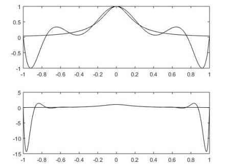
We actually have already seen the best $L_{\infty}$ approximation from $\mathbb{P}{n}[x]$. It is the interpolating polynomial where the interpolation points are chosen to be the Chebyshev points. This is why the best approximation with regards to the $L{\infty}$ norm is sometimes called the Chebyshev approximation. It is also known as Minimax approximation, since the problem can be rephrased as finding $g$ such that
$$
\min {g} \max {x \in[a, b]}|f(x)-g(x)| .
$$

数值分析代写

统计代写|数值分析和优化代写numerical analysis and optimazation代考|Lagrange Form of Polynomial Interpolation

最简单的情况是找到一条直线
p(X)=一种1X+一种0
通过给定的一对点(X0,F0)和(X1,F1). 这意味着求解 2 个方程，每个数据点一个。因此我们有 2 个自由度。对于二次曲线有 3 个自由度，拟合三次曲线我们有 4 个自由度，依此类推。

让磷n[X]最多表示所有实数多项式的线性空间n. 每个p∈磷n[X]由其唯一定义n+1系数。这给n+1自由度，同时插值X0,X1,…,Xn引起n+1条件。

正如我们上面提到的，在确定多项式插值时，我们可以求解线性方程组。然而，这可以更容易地完成。
定义 3.1（拉格朗日基数多项式）。这些是由
大号ķ(X):=∏l=0 l≠ķnX−XlXķ−Xl,X∈R

请注意，拉格朗日基数多项式位于磷n[X]. 很容易验证大号ķ(Xķ)=1和大号ķ(Xj)=0为了j≠ķ. 插值然后由拉格朗日公式给出
p(X)=∑ķ=0nFķ大号ķ(X)=∑ķ=0nFķ∏l=0 l≠ķnX−XlXķ−Xl.
练习 3.1。让函数值F(0),F(1),F(2)， 和F(3)被给予。我们想估计
F(−1),F′(1) 和 ∫03F(X)dX.
为此，我们让p是插值这些函数值的三次多项式，然后近似为
p(−1),p′(1) 和 ∫03p(X)dX
使用拉格朗日公式，证明每个近似值都是具有常数系数的函数值的线性组合，并计算这些系数。证明近似值是精确的，如果F是任何三次多项式。

统计代写|数值分析和优化代写numerical analysis and optimazation代考|Newton Form of Polynomial Interpolation

牛顿介绍了另一种描述多项式插值的方法。然而，首先我们需要介绍一些概念。

定义3.2（分差）。给定成对不同的点X0,X1,…,Xn∈[一种,b]， 让p∈磷n[X]插F∈C米[一种,b]在这些点上。系数Xn在p称为分度差n并表示为F[X0,X1,…,Xn].
从拉格朗日公式我们可以看出
F[X0,X1,…,Xn]=∑ķ=0nF(Xķ)∏l=0 l≠ķn1Xķ−Xl
定理 3.2。那里存在X∈[一种,b]这样
F[X0,X1,…,Xn]=1n!F(n)(X).
证明。让p是多项式插值。区别F−p至少有n+1零。通过应用罗尔定理n次，因此nth 衍生物F(n)−p(n)在某些时候为零X∈[一种,b]. 自从p有学位n,p(n)是恒定的，比如说C，我们有F(n)(X)=C. 另一方面，系数Xn在p是（谁）给的1n!C，因为nth 的导数Xn是n!. 因此我们有
F[X0,X1,…,Xn]=1n!C=1n!F(n)(X)
因此，划分的差异可用于近似导数。

统计代写|数值分析和优化代写numerical analysis and optimazation代考|Polynomial Best Approximations

我们现在将注意力转向最佳近似值，其中最佳值由我们试图最小化的范数（可能由标量积引入）定义。回想一下，标量或内积是任何函数在×R， 在哪里在是一个实向量空间，服从三个公理
对称：
⟨X,是⟩=⟨是,X⟩ 对全部 X,是∈在,
非消极性：
⟨X,X⟩≥0对全部X∈在和⟨X,X⟩=0当且仅当X=0，和
线性：
⟨一种X+b是,和⟩=一种⟨X,和⟩+b⟨是,和⟩ 对全部 X,是,和∈在,一种,b∈R. 
我们已经遇到了向量空间Rn及其与矩阵的 QR 分解的标量积。向量空间的另一个例子是多项式空间n,磷n[X]，但到目前为止还没有为它定义标量积。

一旦定义了标量积，我们就可以定义正交性：X,是∈在是正交的，如果⟨X,是⟩=0. 一个规范可以定义为
|X|=⟨X,X⟩X∈在.
为了在=C[一种,b], 区间上所有连续函数的空间[一种,b]，我们可以使用固定的正函数定义标量积在∈C[一种,b], 权重函数, 方式如下
⟨F,G⟩:=∫一种b在(X)F(X)G(X)dX 对全部 F,G∈C[一种,b].
对于这个标量积，所有三个公理都很容易验证。相关的规范是
|F|2=⟨F,F⟩=∫一种b在(X)F2(X)dX.

为了在(X)≡1这被称为大号2-规范。注意磷n是一个子空间C[一种,b]. 一般来说大号p规范定义为
|F|p=(∫一种b|F(X)|pdX)1/p
存在该积分的函数的向量空间表示为大号p. 除非p=2，这是一个范数空间，但不是一个内积空间，因为这个范数不满足由给出的平行四边形等式
2|F|p2+2|G|p2=|F+G|p2+|F−G|p2
规范需要有一个相关的内积。
让G是函数的近似值F. 经常G被选择位于某个子空间中，例如某个次数的多项式空间。最佳近似选择G这样误差的范数|F−G|被最小化。范数的不同选择给出不同的近似值。
为了p→∞规范变成
|F|∞=最大限度X∈[一种,b]|F(X)|.
我们实际上已经看到了最好的大号∞从近似磷n[X]. 它是插值多项式，其中插值点被选为切比雪夫点。这就是为什么关于大号∞范数有时称为切比雪夫近似。它也被称为 Minimax 逼近，因为这个问题可以重新表述为G这样
分钟G最大限度X∈[一种,b]|F(X)−G(X)|.

统计代写请认准statistics-lab™. statistics-lab™为您的留学生涯保驾护航。统计代写|python代写代考

随机过程代考

在概率论概念中，随机过程是随机变量的集合。 若一随机系统的样本点是随机函数，则称此函数为样本函数，这一随机系统全部样本函数的集合是一个随机过程。 实际应用中，样本函数的一般定义在时间域或者空间域。 随机过程的实例如股票和汇率的波动、语音信号、视频信号、体温的变化，随机运动如布朗运动、随机徘徊等等。

贝叶斯方法代考

贝叶斯统计概念及数据分析表示使用概率陈述回答有关未知参数的研究问题以及统计范式。后验分布包括关于参数的先验分布，和基于观测数据提供关于参数的信息似然模型。根据选择的先验分布和似然模型，后验分布可以解析或近似，例如，马尔科夫链蒙特卡罗 (MCMC) 方法之一。贝叶斯统计概念及数据分析使用后验分布来形成模型参数的各种摘要，包括点估计，如后验平均值、中位数、百分位数和称为可信区间的区间估计。此外，所有关于模型参数的统计检验都可以表示为基于估计后验分布的概率报表。

广义线性模型代考

广义线性模型（GLM）归属统计学领域，是一种应用灵活的线性回归模型。该模型允许因变量的偏差分布有除了正态分布之外的其它分布。

statistics-lab作为专业的留学生服务机构，多年来已为美国、英国、加拿大、澳洲等留学热门地的学生提供专业的学术服务，包括但不限于Essay代写，Assignment代写，Dissertation代写，Report代写，小组作业代写，Proposal代写，Paper代写，Presentation代写，计算机作业代写，论文修改和润色，网课代做，exam代考等等。写作范围涵盖高中，本科，研究生等海外留学全阶段，辐射金融，经济学，会计学，审计学，管理学等全球99%专业科目。写作团队既有专业英语母语作者，也有海外名校硕博留学生，每位写作老师都拥有过硬的语言能力，专业的学科背景和学术写作经验。我们承诺100%原创，100%专业，100%准时，100%满意。

机器学习代写

随着AI的大潮到来，Machine Learning逐渐成为一个新的学习热点。同时与传统CS相比，Machine Learning在其他领域也有着广泛的应用，因此这门学科成为不仅折磨CS专业同学的“小恶魔”，也是折磨生物、化学、统计等其他学科留学生的“大魔王”。学习Machine learning的一大绊脚石在于使用语言众多，跨学科范围广，所以学习起来尤其困难。但是不管你在学习Machine Learning时遇到任何难题，StudyGate专业导师团队都能为你轻松解决。

多元统计分析代考

基础数据: $N$ 个样本， $P$ 个变量数的单样本，组成的横列的数据表
变量定性: 分类和顺序；变量定量：数值
数学公式的角度分为: 因变量与自变量

时间序列分析代写

随机过程，是依赖于参数的一组随机变量的全体，参数通常是时间。 随机变量是随机现象的数量表现，其时间序列是一组按照时间发生先后顺序进行排列的数据点序列。通常一组时间序列的时间间隔为一恒定值（如1秒，5分钟，12小时，7天，1年），因此时间序列可以作为离散时间数据进行分析处理。研究时间序列数据的意义在于现实中，往往需要研究某个事物其随时间发展变化的规律。这就需要通过研究该事物过去发展的历史记录，以得到其自身发展的规律。

回归分析代写

多元回归分析渐进（Multiple Regression Analysis Asymptotics）属于计量经济学领域，主要是一种数学上的统计分析方法，可以分析复杂情况下各影响因素的数学关系，在自然科学、社会和经济学等多个领域内应用广泛。

MATLAB代写

MATLAB 是一种用于技术计算的高性能语言。它将计算、可视化和编程集成在一个易于使用的环境中，其中问题和解决方案以熟悉的数学符号表示。典型用途包括：数学和计算算法开发建模、仿真和原型制作数据分析、探索和可视化科学和工程图形应用程序开发，包括图形用户界面构建MATLAB 是一个交互式系统，其基本数据元素是一个不需要维度的数组。这使您可以解决许多技术计算问题，尤其是那些具有矩阵和向量公式的问题，而只需用 C 或 Fortran 等标量非交互式语言编写程序所需的时间的一小部分。MATLAB 名称代表矩阵实验室。MATLAB 最初的编写目的是提供对由 LINPACK 和 EISPACK 项目开发的矩阵软件的轻松访问，这两个项目共同代表了矩阵计算软件的最新技术。MATLAB 经过多年的发展，得到了许多用户的投入。在大学环境中，它是数学、工程和科学入门和高级课程的标准教学工具。在工业领域，MATLAB 是高效研究、开发和分析的首选工具。MATLAB 具有一系列称为工具箱的特定于应用程序的解决方案。对于大多数 MATLAB 用户来说非常重要，工具箱允许您学习和应用专业技术。工具箱是 MATLAB 函数（M 文件）的综合集合，可扩展 MATLAB 环境以解决特定类别的问题。可用工具箱的领域包括信号处理、控制系统、神经网络、模糊逻辑、小波、仿真等。

R语言代写	问卷设计与分析代写
PYTHON代写	回归分析与线性模型代写
MATLAB代写	方差分析与试验设计代写
STATA代写	机器学习/统计学习代写
SPSS代写	计量经济学代写
EVIEWS代写	时间序列分析代写
EXCEL代写	深度学习代写
SQL代写	各种数据建模与可视化代写

如果你也在 怎样代写数值分析和优化numerical analysis and optimazation这个学科遇到相关的难题，请随时右上角联系我们的24/7代写客服。

数值分析是根据数学模型提出的问题，建立求解问题的数值计算方法并进行方法的理论分析，直到编制出算法程序上机计算得到数值结果，以及对结果进行分析。

statistics-lab™ 为您的留学生涯保驾护航 在代写数值分析和优化numerical analysis and optimazation方面已经树立了自己的口碑, 保证靠谱, 高质且原创的统计Statistics代写服务。我们的专家在代写数值分析和优化numerical analysis and optimazation方面经验极为丰富，各种代写数值分析和优化numerical analysis and optimazation相关的作业也就用不着说。

我们提供的数值分析和优化numerical analysis and optimazation及其相关学科的代写，服务范围广, 其中包括但不限于:

• Statistical Inference 统计推断
• Statistical Computing 统计计算
• Advanced Probability Theory 高等楖率论
• Advanced Mathematical Statistics 高等数理统计学
• (Generalized) Linear Models 广义线性模型
• Statistical Machine Learning 统计机器学习
• Longitudinal Data Analysis 纵向数据分析
• Foundations of Data Science 数据科学基础

统计代写|数值分析和优化代写numerical analysis and optimazation代考|The Power Method

The power method forms the basic of many iterative algorithms for the calculation of eigenvalues and eigenvectors. It generates a single eigenvector and eigenvalue of $A$.

1. Pick a starting vector $\mathbf{x}^{(0)} \in \mathbb{R}^{n}$ satisfying $\left|\mathbf{x}^{(0)}\right|=1$. Set $k=0$ and choose a tolerance $\epsilon>0$.
2. Calculate $\mathbf{x}^{(k+1)}=A \mathbf{x}^{(k)}$ and find the real number $\lambda$ that minimizes

$\left|\mathbf{x}^{(k+1)}-\lambda \mathbf{x}^{(k)}\right|$. This is given by the Rayleigh quotient
$$
\lambda=\frac{\mathbf{x}^{(k)^{T}} A \mathbf{x}^{(k)}}{\mathbf{x}^{(k)^{T}} \mathbf{x}^{(k)}} .
$$

3. Accept $\lambda$ as an eigenvalue and $\mathbf{x}^{(k)}$ as an eigenvector , if $| \mathbf{x}^{(k+1)}-$ $\lambda \mathbf{x}^{(k)} | \leq \epsilon$.
4. Otherwise, replace $\mathbf{x}^{(k+1)}$ by $\mathbf{x}^{(k+1)} /\left|\mathbf{x}^{(k+1)}\right|$, increase $k$ by one, and go back to step $2 .$

统计代写|数值分析和优化代写numerical analysis and optimazation代考|Inverse Iteration

The method described in this section is called inverse iteration and is very effective in practice. It is similar to the power method with shifts, except that, instead of $\mathbf{x}^{(k+1)}$ being a multiple of $(A-s I) \mathbf{x}^{(k)}$, it is calculated as a scalar multiple of the solution to
$$
(A-s I) \mathbf{x}^{(k+1)}=\mathbf{x}^{(k)}, \quad k=0,1, \ldots
$$
where $s$ is a scalar that may depend on $k$. Thus the inverse power method is the power method applied to the matrix $(A-s I)^{-1}$. If $s$ is close to an eigenvalue, then the matrix $A-s I$ has an eigenvalue close to zero, but this implies that $(A-s I)^{-1}$ has a very large eigenvalue and we have seen that in this case the power method converges fast.

In every iteration $\mathbf{x}^{(k+1)}$ is scaled such that $\left|\mathbf{x}^{(k+1)}\right|=1$. We see that the calculation of $\mathbf{x}^{(k+1)}$ requires the solution of an $n \times n$ system of equations.
If $s$ is constant in every iteration such that $A-s I$ is nonsingular, then $\mathbf{x}^{(k+1)}$ is a multiple of $(A-s I)^{-k-1} \mathbf{x}^{(0)}$. As before we let $\mathbf{x}^{(0)}=\sum_{j=1}^{n} c_{j} \mathbf{v}{j}$, where $\mathbf{v}{j}, j=1, \ldots, n$, are the linearly independent eigenvectors. The eigenvalue equation then implies $(A-s I) \mathbf{v}{j}=\left(\lambda{j}-s\right) \mathbf{v}{j}$. For the inverse we have then $(A-s I)^{-1} \mathbf{v}{j}=\left(\lambda_{j}-s\right)^{-1} \mathbf{v}{j}$. It follows that $\mathbf{x}^{(k+1)}$ is a multiple of $$ (A-s I)^{-k-1} \mathbf{x}^{(0)}=\sum{j=0}^{n} c_{j}(A-s I)^{-k-1} \mathbf{v}{j}=\sum{j=0}^{n} c_{j}\left(\lambda_{j}-s\right)^{-k-1} \mathbf{v}{j} $$ Let $m$ be the index of the smallest number of $\left|\lambda{j}-s\right| \cdot j=1, \ldots, n$. If $c_{m}$ is nonzero then $\mathbf{x}^{(k+1)}$ tends to be multiple of $\mathbf{v}_{m}$ as $k$ tends to infinity. The speed of convergence can be excellent if $s$ is close to $\lambda_{m}$. It can be improved even more if $s$ is adjusted during the iterations as the following implementation shows.

统计代写|数值分析和优化代写numerical analysis and optimazation代考|Deflation

Suppose we have found one solution of the eigenvector equation $A \mathbf{v}=\lambda \mathbf{v}$ (or possibly a pair of complex conjugate eigenvalues with their corresponding eigenvectors), where $A$ is an $n \times n$ matrix. Deflation constructs an $(n-1) \times$ $(n-1)$ (or $(n-2) \times(n-2)$ ) matrix, say $B$, whose eigenvalues are the other $n-1$ (or $n-2$ ) eigenvalues of $A$. The concept is based on the following theorem.
Theorem 2.12. Let $A$ and $S$ be $n \times n$ matrices, $S$ being nonsingular. Then $\mathbf{v}$ is an eigenvector of $A$ with eigenvalue $\lambda$ if and only if $S \mathbf{v}$ is an eigenvector of $S A S^{-1}$ with the same eigenvalue. $S$ is called a similarity transformation.
Proof.
$$
A \mathbf{v}=\lambda \mathbf{v} \Leftrightarrow A S^{-1}(S \mathbf{v})=\lambda \mathbf{v} \Leftrightarrow\left(S A S^{-1}\right)(S \mathbf{v})=\lambda(S \mathbf{v})
$$
Let’s assume one eigenvalue $\lambda$ and its corresponding eigenvector have been found. In deflation we apply a similarity transformation $S$ to $A$ such that the first column of $S A S^{-1}$ is $\lambda$ times the first standard unit vector $\mathbf{e}{1}$, $$ \left(S A S^{-1}\right) \mathbf{e}{1}=\lambda \mathbf{e}{1} . $$ Then we can let $B$ be the bottom right $(n-1) \times(n-1)$ submatrix of $S A S^{-1}$. We see from the above theorem that it is sufficient to let $S$ have the property $S \mathbf{v}=a \mathbf{e}{1}$, where $a$ is any nonzero scalar.

If we know a complex conjugate pair of eigenvalues, then there is a twodimensional eigenspace associated with them. Eigenspace means that if $A$ is applied to any vector in the eigenspace, then the result will again lie in the eigenspace. Let $\mathbf{v}{1}$ and $\mathbf{v}{2}$ be vectors spanning the eigenspace. For example these could have been found by the two-stage power method. We need to find a similarity transformation $S$ which maps the eigenspace to the space spanned by the first two standard basis vectors $\mathbf{e}{1}$ and $\mathbf{e}{2}$. Let $S_{1}$ such that $S_{1} \mathbf{v}{1}=a \mathbf{e}{1}$. In addition let $\hat{\mathbf{v}}$ be the vector composed of the last $n-1$ components of $S_{1} \mathbf{v}{2}$. We then let $S{2}$ be of the form
$$
S_{2}=\left(\begin{array}{cccc}
1 & 0 & \cdots & 0 \
0 & & & \
\vdots & & \hat{S} & \
0 & & &
\end{array}\right),
$$

数值分析代写

统计代写|数值分析和优化代写numerical analysis and optimazation代考|The Power Method

幂法构成了许多用于计算特征值和特征向量的迭代算法的基础。它生成单个特征向量和特征值一种.

1. 选择一个起始向量X(0)∈Rn令人满意的|X(0)|=1. 放ķ=0并选择一个公差ε>0.
2. 计算X(ķ+1)=一种X(ķ)并找到实数λ最小化

|X(ķ+1)−λX(ķ)|. 这是由瑞利商给出的
λ=X(ķ)吨一种X(ķ)X(ķ)吨X(ķ).

3. 接受λ作为特征值和X(ķ)作为一个特征向量，如果|X(ķ+1)− λX(ķ)|≤ε.
4. 否则，更换X(ķ+1)经过X(ķ+1)/|X(ķ+1)|， 增加ķ减一，然后返回步骤2.

统计代写|数值分析和优化代写numerical analysis and optimazation代考|Inverse Iteration

本节介绍的方法称为逆迭代，在实践中非常有效。它类似于带班次的幂法，不同之处在于，它不是X(ķ+1)是的倍数(一种−s一世)X(ķ)，它被计算为解的标量倍数
(一种−s一世)X(ķ+1)=X(ķ),ķ=0,1,…
在哪里s是一个标量，可能取决于ķ. 因此逆幂法是应用于矩阵的幂法(一种−s一世)−1. 如果s接近特征值，则矩阵一种−s一世具有接近于零的特征值，但这意味着(一种−s一世)−1有一个非常大的特征值，我们已经看到，在这种情况下，幂方法收敛得很快。

在每一次迭代中X(ķ+1)被缩放使得|X(ķ+1)|=1. 我们看到计算X(ķ+1)需要一个解决方案n×n方程组。
如果s在每次迭代中都是常数，使得一种−s一世是非奇异的，那么X(ķ+1)是的倍数(一种−s一世)−ķ−1X(0). 和以前一样，我们让X(0)=∑j=1nCj在j， 在哪里在j,j=1,…,n, 是线性独立的特征向量。然后特征值方程意味着(一种−s一世)在j=(λj−s)在j. 对于逆我们有(一种−s一世)−1在j=(λj−s)−1在j. 它遵循X(ķ+1)是的倍数(一种−s一世)−ķ−1X(0)=∑j=0nCj(一种−s一世)−ķ−1在j=∑j=0nCj(λj−s)−ķ−1在j让米是最小数量的索引|λj−s|⋅j=1,…,n. 如果C米那么是非零的X(ķ+1)往往是倍数在米作为ķ趋于无穷大。收敛速度可以是极好的，如果s接近λ米. 它可以进一步改进，如果s在迭代期间进行调整，如下面的实现所示。

统计代写|数值分析和优化代写numerical analysis and optimazation代考|Deflation

假设我们找到了特征向量方程的一个解一种在=λ在（或者可能是一对复共轭特征值及其对应的特征向量），其中一种是一个n×n矩阵。通货紧缩构造了一个(n−1)× (n−1)（或者(n−2)×(n−2)) 矩阵，比如说乙，其特征值是另一个n−1（或者n−2) 的特征值一种. 该概念基于以下定理。
定理 2.12。让一种和小号是n×n矩阵，小号是非奇异的。然后在是一个特征向量一种有特征值λ当且仅当小号在是一个特征向量小号一种小号−1具有相同的特征值。小号称为相似变换。
证明。
一种在=λ在⇔一种小号−1(小号在)=λ在⇔(小号一种小号−1)(小号在)=λ(小号在)
让我们假设一个特征值λ及其对应的特征向量已经找到。在通货紧缩中，我们应用相似变换小号到一种使得第一列小号一种小号−1是λ乘以第一个标准单位向量和1,(小号一种小号−1)和1=λ和1.然后我们可以让乙成为右下角(n−1)×(n−1)的子矩阵小号一种小号−1. 我们从上面的定理看出，让小号拥有财产小号在=一种和1， 在哪里一种是任何非零标量。

如果我们知道一个复共轭特征值对，那么就有一个与它们相关的二维特征空间。特征空间意味着如果一种应用于特征空间中的任何向量，则结果将再次位于特征空间中。让在1和在2是跨越特征空间的向量。例如，这些可以通过两级功率方法找到。我们需要找到一个相似变换小号它将特征空间映射到前两个标准基向量所跨越的空间和1和和2. 让小号1这样小号1在1=一种和1. 另外让在^是由最后一个组成的向量n−1的组成部分小号1在2. 然后我们让小号2成为形式
小号2=(10⋯0 0 ⋮小号^ 0),

统计代写请认准statistics-lab™. statistics-lab™为您的留学生涯保驾护航。统计代写|python代写代考

随机过程代考

在概率论概念中，随机过程是随机变量的集合。 若一随机系统的样本点是随机函数，则称此函数为样本函数，这一随机系统全部样本函数的集合是一个随机过程。 实际应用中，样本函数的一般定义在时间域或者空间域。 随机过程的实例如股票和汇率的波动、语音信号、视频信号、体温的变化，随机运动如布朗运动、随机徘徊等等。

贝叶斯方法代考

贝叶斯统计概念及数据分析表示使用概率陈述回答有关未知参数的研究问题以及统计范式。后验分布包括关于参数的先验分布，和基于观测数据提供关于参数的信息似然模型。根据选择的先验分布和似然模型，后验分布可以解析或近似，例如，马尔科夫链蒙特卡罗 (MCMC) 方法之一。贝叶斯统计概念及数据分析使用后验分布来形成模型参数的各种摘要，包括点估计，如后验平均值、中位数、百分位数和称为可信区间的区间估计。此外，所有关于模型参数的统计检验都可以表示为基于估计后验分布的概率报表。

广义线性模型代考

广义线性模型（GLM）归属统计学领域，是一种应用灵活的线性回归模型。该模型允许因变量的偏差分布有除了正态分布之外的其它分布。

statistics-lab作为专业的留学生服务机构，多年来已为美国、英国、加拿大、澳洲等留学热门地的学生提供专业的学术服务，包括但不限于Essay代写，Assignment代写，Dissertation代写，Report代写，小组作业代写，Proposal代写，Paper代写，Presentation代写，计算机作业代写，论文修改和润色，网课代做，exam代考等等。写作范围涵盖高中，本科，研究生等海外留学全阶段，辐射金融，经济学，会计学，审计学，管理学等全球99%专业科目。写作团队既有专业英语母语作者，也有海外名校硕博留学生，每位写作老师都拥有过硬的语言能力，专业的学科背景和学术写作经验。我们承诺100%原创，100%专业，100%准时，100%满意。

机器学习代写

随着AI的大潮到来，Machine Learning逐渐成为一个新的学习热点。同时与传统CS相比，Machine Learning在其他领域也有着广泛的应用，因此这门学科成为不仅折磨CS专业同学的“小恶魔”，也是折磨生物、化学、统计等其他学科留学生的“大魔王”。学习Machine learning的一大绊脚石在于使用语言众多，跨学科范围广，所以学习起来尤其困难。但是不管你在学习Machine Learning时遇到任何难题，StudyGate专业导师团队都能为你轻松解决。

多元统计分析代考

基础数据: $N$ 个样本， $P$ 个变量数的单样本，组成的横列的数据表
变量定性: 分类和顺序；变量定量：数值
数学公式的角度分为: 因变量与自变量

时间序列分析代写

随机过程，是依赖于参数的一组随机变量的全体，参数通常是时间。 随机变量是随机现象的数量表现，其时间序列是一组按照时间发生先后顺序进行排列的数据点序列。通常一组时间序列的时间间隔为一恒定值（如1秒，5分钟，12小时，7天，1年），因此时间序列可以作为离散时间数据进行分析处理。研究时间序列数据的意义在于现实中，往往需要研究某个事物其随时间发展变化的规律。这就需要通过研究该事物过去发展的历史记录，以得到其自身发展的规律。

回归分析代写

多元回归分析渐进（Multiple Regression Analysis Asymptotics）属于计量经济学领域，主要是一种数学上的统计分析方法，可以分析复杂情况下各影响因素的数学关系，在自然科学、社会和经济学等多个领域内应用广泛。

MATLAB代写

MATLAB 是一种用于技术计算的高性能语言。它将计算、可视化和编程集成在一个易于使用的环境中，其中问题和解决方案以熟悉的数学符号表示。典型用途包括：数学和计算算法开发建模、仿真和原型制作数据分析、探索和可视化科学和工程图形应用程序开发，包括图形用户界面构建MATLAB 是一个交互式系统，其基本数据元素是一个不需要维度的数组。这使您可以解决许多技术计算问题，尤其是那些具有矩阵和向量公式的问题，而只需用 C 或 Fortran 等标量非交互式语言编写程序所需的时间的一小部分。MATLAB 名称代表矩阵实验室。MATLAB 最初的编写目的是提供对由 LINPACK 和 EISPACK 项目开发的矩阵软件的轻松访问，这两个项目共同代表了矩阵计算软件的最新技术。MATLAB 经过多年的发展，得到了许多用户的投入。在大学环境中，它是数学、工程和科学入门和高级课程的标准教学工具。在工业领域，MATLAB 是高效研究、开发和分析的首选工具。MATLAB 具有一系列称为工具箱的特定于应用程序的解决方案。对于大多数 MATLAB 用户来说非常重要，工具箱允许您学习和应用专业技术。工具箱是 MATLAB 函数（M 文件）的综合集合，可扩展 MATLAB 环境以解决特定类别的问题。可用工具箱的领域包括信号处理、控制系统、神经网络、模糊逻辑、小波、仿真等。

R语言代写	问卷设计与分析代写
PYTHON代写	回归分析与线性模型代写
MATLAB代写	方差分析与试验设计代写
STATA代写	机器学习/统计学习代写
SPSS代写	计量经济学代写
EVIEWS代写	时间序列分析代写
EXCEL代写	深度学习代写
SQL代写	各种数据建模与可视化代写

如果你也在 怎样代写数值分析和优化numerical analysis and optimazation这个学科遇到相关的难题，请随时右上角联系我们的24/7代写客服。

数值分析是根据数学模型提出的问题，建立求解问题的数值计算方法并进行方法的理论分析，直到编制出算法程序上机计算得到数值结果，以及对结果进行分析。

statistics-lab™ 为您的留学生涯保驾护航 在代写数值分析和优化numerical analysis and optimazation方面已经树立了自己的口碑, 保证靠谱, 高质且原创的统计Statistics代写服务。我们的专家在代写数值分析和优化numerical analysis and optimazation方面经验极为丰富，各种代写数值分析和优化numerical analysis and optimazation相关的作业也就用不着说。

我们提供的数值分析和优化numerical analysis and optimazation及其相关学科的代写，服务范围广, 其中包括但不限于:

• Statistical Inference 统计推断
• Statistical Computing 统计计算
• Advanced Probability Theory 高等楖率论
• Advanced Mathematical Statistics 高等数理统计学
• (Generalized) Linear Models 广义线性模型
• Statistical Machine Learning 统计机器学习
• Longitudinal Data Analysis 纵向数据分析
• Foundations of Data Science 数据科学基础

统计代写|数值分析和优化代写numerical analysis and optimazation代考|Conjugate Gradients

We have already seen how the positive definiteness of $A$ can be used to define a norm. This can be extended to have a concept similar to orthogonality.
Definition 2.8. The vectors $\mathbf{u}$ and $\mathbf{v}$ are conjugate with respect to the positive definite matrix $A$, if they are nonzero and satisfy $\mathbf{u}^{T} A \mathbf{v}=0$.

Conjugacy plays such an important role, because through it search directions can be constructed such that the new gradient $\mathbf{g}^{(k+1)}$ is not just orthogonal to the current search direction $\mathbf{d}^{(k)}$ but to all previous search directions. This avoids revisiting search directions as in Figure 2.1.

Specifically, the first search direction is chosen as $\mathbf{d}^{(0)}=-\mathbf{g}^{(0)}$. The following search directions are then constructed by
$$
\mathbf{d}^{(k)}=-\mathbf{g}^{(k)}+\beta^{(k)} \mathbf{d}^{(k-1)}, \quad k=1,2, \ldots,
$$
where $\beta^{(k)}$ is chosen such that the conjugacy condition $\mathbf{d}^{(k)^{T}} A \mathbf{d}^{(k-1)}=0$ is satisfied. This yields
$$
\beta^{(k)}=\frac{\mathbf{g}^{(k)^{T}} A \mathbf{d}^{(k-1)}}{\mathbf{d}^{(k-1)^{T}} A \mathbf{d}^{(k-1)}}, \quad k=1,2, \ldots
$$
This gives the conjugate gradient method.
The values of $\mathbf{x}^{(k+1)}$ and $\omega^{(k)}$ are calculated as before in (2.7) and $(2.9)$.
These search directions satisfy the descent condition. From Equation (2.8) we have seen that the descent condition is equivalent to $\mathbf{d}^{(k)^{T}} \mathbf{g}^{(k)}<0$. Using the formula for $\mathbf{d}^{(k)}$ above and the fact that the new gradient is orthogonal to the previous search direction, i.e., $\mathbf{d}^{(k-1)^{T}} \mathbf{g}^{(k)}=0$, we see that
$$
\mathbf{d}^{(k)^{T}} \mathbf{g}^{(k)}=-\left|\mathbf{g}^{(k)}\right|^{2}<0
$$

统计代写|数值分析和优化代写numerical analysis and optimazation代考|Krylov Subspaces and Pre-Conditioning

Definition 2.9. Let $A$ be an $n \times n$ matrix, $\mathbf{b} \in \mathbb{R}^{n}$ a non-zero vector, then for a number $m$ the space spanned by $A^{j} \mathbf{b}, j=0, \ldots, m-1$ is the $m^{\text {th }}$ Krylov subspace of $\mathbb{R}^{n}$ and is denoted by $K_{m}(A, \mathbf{b})$.

In our analysis of the conjugate gradient method we saw that in the $k^{\text {th }}$ iteration the space spanned by the search directions $\mathbf{d}^{(j)}$ and the space spanned by the gradients $\mathbf{g}^{(j)}, j=0, \ldots, k$, are the same.

Lemma 2.3. The space spanned by $\mathbf{g}^{(j)}\left(\right.$ or $\left.\mathbf{d}^{(j)}\right), j=0, \ldots, k$, is the same as the $k+1^{\text {th }}$ Krylov subspace.
Proof. For $k=0$ we have $\mathbf{d}^{(0)}=-\mathbf{g}^{(0)}=\mathbf{b} \in K_{1}(A, \mathbf{b})$.
We assume that the space spanned by $\mathbf{g}^{(j)}, j=0, \ldots, k$, is the same as the space spanned by $\mathbf{b}, A \mathbf{b}, \ldots, A^{k} \mathbf{b}$ and increase $k$ by one.

In the formula $\mathbf{g}^{(k+1)}=\mathbf{g}^{(k)}+\omega^{(k)} A \mathbf{d}^{(k)}$ both $\mathbf{g}^{(k)}$ and $\mathbf{d}^{(k)}$ can be expressed as linear combinations of $\mathbf{b}, A \mathbf{b}, \ldots, A^{k} \mathbf{b}$ by the inductive hypothesis. Thus $\mathbf{g}^{(k+1)}$ can be expressed as a linear combination of $\mathbf{b}, A \mathbf{b}, \ldots, A^{k+1} \mathbf{b}$. Equally, using $\mathbf{d}^{(k+1)}=-\mathbf{g}^{(k+1)}+\beta^{(k)} \mathbf{d}^{(k)}$ we show that $\mathbf{d}^{(k+1)}$ lies in the space spanned by b, $A \mathbf{b}, \ldots, A^{k+1} \mathbf{b}$, which is $K_{k+2}(A, \mathbf{b})$. This completes the proof.

In the following lemma we show some properties of the Krylov subspaces.
Lemma 2.4. Given $A$ and b. Then $K_{m}(A, \mathbf{b})$ is a subspace of $K_{m+1}(A, \mathbf{b})$ and there exists a positive integer $s \leq n$ such that for every $m \geq s K_{m}(A, \mathbf{b})=$ $K_{s}(A, \mathbf{b})$. Furthermore, if we express $\mathbf{b}$ as $\mathbf{b}=\sum_{i=1}^{t} c_{i} \mathbf{v}{i}$, where $\mathbf{v}{1}, \ldots, \mathbf{v}{t}$ are eigenvectors of $A$ corresponding to distinct eigenvalues and all coefficients $c{i}, i=1, \ldots, t$, are non-zero, then $s=t$.

Proof. Clearly, $K_{m}(A, \mathbf{b}) \subseteq K_{m+1}(A, \mathbf{b})$. The dimension of $K_{m}(A, \mathbf{b})$ is less than or equal to $m$, since it is spanned by $m$ vectors. It is also at most $n$ since

$K_{m}(A, \mathbf{b})$ is a subspace of $\mathbb{R}^{n}$. The first Krylov subspace has dimension 1 . We let $s$ be the greatest integer such that the dimension of $K_{s}(A, \mathbf{b})$ is $s$. Then the dimension of $K_{s+1}(A, \mathbf{b})$ cannot be $s+1$ by the choice of $s$. It has to be $s$, since $K_{s}(A, \mathbf{b}) \subseteq K_{s+1}(A, \mathbf{b})$. Hence the two spaces are the same. This means that $A^{s} \mathbf{b} \in K_{s}(A, \mathbf{b})$, i.e., $A^{s} \mathbf{b}=\sum_{j=0}^{s-1} a_{j} A^{j} \mathbf{b}$. But then
$$
A^{s+r} \mathbf{b}=\sum_{j=0}^{s-1} a_{j} A^{j+r} \mathbf{b}
$$
for any positive $r$. This means that also the spaces $K_{s+r+1}(A$, b $)$ and $K_{s+r}(A, \mathbf{b})$ are the same. Therefore, for every $m \geq s K_{m}(A, \mathbf{b})=K_{s}(A, \mathbf{b})$.
Suppose now that $\mathbf{b}=\sum_{i=1}^{t} c_{i} \mathbf{v}{i}$, where $\mathbf{v}{1}, \ldots, \mathbf{v}{t}$ are eigenvectors of $A$ corresponding to distinct eigenvalues $\lambda{i}$. Then for every $j=1, \ldots, s$
$$
A^{j} \mathbf{b}=\sum_{i=1}^{t} c_{i} \lambda_{i}^{j} \mathbf{v}_{i}
$$

统计代写|数值分析和优化代写numerical analysis and optimazation代考|Eigenvalues and Eigenvectors

So far we only considered eigenvalues when analyzing the properties of numerical methods. In the following sections we look at how to determine eigenvalues and eigenvectors. Let $A$ be a real $n \times n$ matrix. The eigenvalue equation is given by
$$
A \mathbf{v}=\lambda \mathbf{v} \text {, }
$$
where $\lambda$ is scalar. It may be complex if $A$ is not symmetric. There exists $\mathbf{v} \in \mathbb{R}^{n}$ satisfying the eigenvalue equation if and only if the determinant $\operatorname{det}(A-\lambda I)$ is zero. The function $p(\lambda)=\operatorname{det}(A-\lambda I), \lambda \in \mathbb{C}$, is a polynomial of degree $n$. However, calculating the eigenvalues by finding the roots of $p$ is generally unsuitable because of loss of accuracy due to rounding errors. In Chapter 1 , Fundamentals, we have seen how even finding the roots of a quadratic can be difficult due to loss of significance.

If the polynomial has some multiple roots and if $A$ is not symmetric, then $A$ might have less than $n$ linearly independent eigenvalues. However, there are always $n$ mutually orthogonal real eigenvectors when $A$ is symmetric. In the following we assume that $A$ has $n$ linearly independent eigenvectors $\mathbf{v}{j}$ for each eigenvalue $\lambda{j}, j=1, \ldots, n$. This can be achieved by perturbing $A$ slightly if necessary. The task is now to find $\mathbf{v}{j}$ and $\lambda{j}, j=1, \ldots, n$.

数值分析代写

统计代写|数值分析和优化代写numerical analysis and optimazation代考|Conjugate Gradients

We have already seen how the positive definiteness of A can be used to define a norm. This can be extended to have a concept similar to orthogonality.
Definition 2.8. The vectors u and v are conjugate with respect to the positive definite matrix A, if they are nonzero and satisfy uTAv=0.

Conjugacy plays such an important role, because through it search directions can be constructed such that the new gradient g(k+1) is not just orthogonal to the current search direction d(k) but to all previous search directions. This avoids revisiting search directions as in Figure 2.1.

Specifically, the first search direction is chosen as d(0)=−g(0). The following search directions are then constructed by
d(k)=−g(k)+β(k)d(k−1),k=1,2,…,
where β(k) is chosen such that the conjugacy condition d(k)TAd(k−1)=0 is satisfied. This yields
β(k)=g(k)TAd(k−1)d(k−1)TAd(k−1),k=1,2,…
This gives the conjugate gradient method.
The values of x(k+1) and ω(k) are calculated as before in (2.7) and (2.9).
These search directions satisfy the descent condition. From Equation (2.8) we have seen that the descent condition is equivalent to d(k)Tg(k)<0. Using the formula for d(k) above and the fact that the new gradient is orthogonal to the previous search direction, i.e., d(k−1)Tg(k)=0, we see that
d(k)Tg(k)=−|g(k)|2<0

统计代写|数值分析和优化代写numerical analysis and optimazation代考|Krylov Subspaces and Pre-Conditioning

Definition 2.9. Let A be an n×n matrix, b∈Rn a non-zero vector, then for a number m the space spanned by Ajb,j=0,…,m−1 is the mth  Krylov subspace of Rn and is denoted by Km(A,b).

In our analysis of the conjugate gradient method we saw that in the kth  iteration the space spanned by the search directions d(j) and the space spanned by the gradients g(j),j=0,…,k, are the same.

Lemma 2.3. The space spanned by g(j)( or d(j)),j=0,…,k, is the same as the k+1th  Krylov subspace.
Proof. For k=0 we have d(0)=−g(0)=b∈K1(A,b).
We assume that the space spanned by g(j),j=0,…,k, is the same as the space spanned by b,Ab,…,Akb and increase k by one.

In the formula g(k+1)=g(k)+ω(k)Ad(k) both g(k) and d(k) can be expressed as linear combinations of b,Ab,…,Akb by the inductive hypothesis. Thus g(k+1) can be expressed as a linear combination of b,Ab,…,Ak+1b. Equally, using d(k+1)=−g(k+1)+β(k)d(k) we show that d(k+1) lies in the space spanned by b, Ab,…,Ak+1b, which is Kk+2(A,b). This completes the proof.

In the following lemma we show some properties of the Krylov subspaces.
Lemma 2.4. Given A and b. Then Km(A,b) is a subspace of Km+1(A,b) and there exists a positive integer s≤n such that for every m≥sKm(A,b)= Ks(A,b). Furthermore, if we express b as b=∑i=1tcivi, where v1,…,vt are eigenvectors of A corresponding to distinct eigenvalues and all coefficients ci,i=1,…,t, are non-zero, then s=t.

Proof. Clearly, Km(A,b)⊆Km+1(A,b). The dimension of Km(A,b) is less than or equal to m, since it is spanned by m vectors. It is also at most n since

Km(A,b) is a subspace of Rn. The first Krylov subspace has dimension 1 . We let s be the greatest integer such that the dimension of Ks(A,b) is s. Then the dimension of Ks+1(A,b) cannot be s+1 by the choice of s. It has to be s, since Ks(A,b)⊆Ks+1(A,b). Hence the two spaces are the same. This means that Asb∈Ks(A,b), i.e., Asb=∑j=0s−1ajAjb. But then
As+rb=∑j=0s−1ajAj+rb
for any positive r. This means that also the spaces Ks+r+1(A, b ) and Ks+r(A,b) are the same. Therefore, for every m≥sKm(A,b)=Ks(A,b).
Suppose now that b=∑i=1tcivi, where v1,…,vt are eigenvectors of A corresponding to distinct eigenvalues λi. Then for every j=1,…,s
Ajb=∑i=1tciλijvi

统计代写|数值分析和优化代写numerical analysis and optimazation代考|Eigenvalues and Eigenvectors

So far we only considered eigenvalues when analyzing the properties of numerical methods. In the following sections we look at how to determine eigenvalues and eigenvectors. Let A be a real n×n matrix. The eigenvalue equation is given by
Av=λv, 
where λ is scalar. It may be complex if A is not symmetric. There exists v∈Rn satisfying the eigenvalue equation if and only if the determinant det⁡(A−λI) is zero. The function p(λ)=det⁡(A−λI),λ∈C, is a polynomial of degree n. However, calculating the eigenvalues by finding the roots of p is generally unsuitable because of loss of accuracy due to rounding errors. In Chapter 1 , Fundamentals, we have seen how even finding the roots of a quadratic can be difficult due to loss of significance.

If the polynomial has some multiple roots and if A is not symmetric, then A might have less than n linearly independent eigenvalues. However, there are always n mutually orthogonal real eigenvectors when A is symmetric. In the following we assume that A has n linearly independent eigenvectors vj for each eigenvalue λj,j=1,…,n. This can be achieved by perturbing A slightly if necessary. The task is now to find vj and λj,j=1,…,n.

统计代写请认准statistics-lab™. statistics-lab™为您的留学生涯保驾护航。统计代写|python代写代考

随机过程代考

在概率论概念中，随机过程是随机变量的集合。 若一随机系统的样本点是随机函数，则称此函数为样本函数，这一随机系统全部样本函数的集合是一个随机过程。 实际应用中，样本函数的一般定义在时间域或者空间域。 随机过程的实例如股票和汇率的波动、语音信号、视频信号、体温的变化，随机运动如布朗运动、随机徘徊等等。

贝叶斯方法代考

贝叶斯统计概念及数据分析表示使用概率陈述回答有关未知参数的研究问题以及统计范式。后验分布包括关于参数的先验分布，和基于观测数据提供关于参数的信息似然模型。根据选择的先验分布和似然模型，后验分布可以解析或近似，例如，马尔科夫链蒙特卡罗 (MCMC) 方法之一。贝叶斯统计概念及数据分析使用后验分布来形成模型参数的各种摘要，包括点估计，如后验平均值、中位数、百分位数和称为可信区间的区间估计。此外，所有关于模型参数的统计检验都可以表示为基于估计后验分布的概率报表。

广义线性模型代考

广义线性模型（GLM）归属统计学领域，是一种应用灵活的线性回归模型。该模型允许因变量的偏差分布有除了正态分布之外的其它分布。

statistics-lab作为专业的留学生服务机构，多年来已为美国、英国、加拿大、澳洲等留学热门地的学生提供专业的学术服务，包括但不限于Essay代写，Assignment代写，Dissertation代写，Report代写，小组作业代写，Proposal代写，Paper代写，Presentation代写，计算机作业代写，论文修改和润色，网课代做，exam代考等等。写作范围涵盖高中，本科，研究生等海外留学全阶段，辐射金融，经济学，会计学，审计学，管理学等全球99%专业科目。写作团队既有专业英语母语作者，也有海外名校硕博留学生，每位写作老师都拥有过硬的语言能力，专业的学科背景和学术写作经验。我们承诺100%原创，100%专业，100%准时，100%满意。

机器学习代写

随着AI的大潮到来，Machine Learning逐渐成为一个新的学习热点。同时与传统CS相比，Machine Learning在其他领域也有着广泛的应用，因此这门学科成为不仅折磨CS专业同学的“小恶魔”，也是折磨生物、化学、统计等其他学科留学生的“大魔王”。学习Machine learning的一大绊脚石在于使用语言众多，跨学科范围广，所以学习起来尤其困难。但是不管你在学习Machine Learning时遇到任何难题，StudyGate专业导师团队都能为你轻松解决。

多元统计分析代考

基础数据: $N$ 个样本， $P$ 个变量数的单样本，组成的横列的数据表
变量定性: 分类和顺序；变量定量：数值
数学公式的角度分为: 因变量与自变量

时间序列分析代写

随机过程，是依赖于参数的一组随机变量的全体，参数通常是时间。 随机变量是随机现象的数量表现，其时间序列是一组按照时间发生先后顺序进行排列的数据点序列。通常一组时间序列的时间间隔为一恒定值（如1秒，5分钟，12小时，7天，1年），因此时间序列可以作为离散时间数据进行分析处理。研究时间序列数据的意义在于现实中，往往需要研究某个事物其随时间发展变化的规律。这就需要通过研究该事物过去发展的历史记录，以得到其自身发展的规律。

回归分析代写

多元回归分析渐进（Multiple Regression Analysis Asymptotics）属于计量经济学领域，主要是一种数学上的统计分析方法，可以分析复杂情况下各影响因素的数学关系，在自然科学、社会和经济学等多个领域内应用广泛。

MATLAB代写

MATLAB 是一种用于技术计算的高性能语言。它将计算、可视化和编程集成在一个易于使用的环境中，其中问题和解决方案以熟悉的数学符号表示。典型用途包括：数学和计算算法开发建模、仿真和原型制作数据分析、探索和可视化科学和工程图形应用程序开发，包括图形用户界面构建MATLAB 是一个交互式系统，其基本数据元素是一个不需要维度的数组。这使您可以解决许多技术计算问题，尤其是那些具有矩阵和向量公式的问题，而只需用 C 或 Fortran 等标量非交互式语言编写程序所需的时间的一小部分。MATLAB 名称代表矩阵实验室。MATLAB 最初的编写目的是提供对由 LINPACK 和 EISPACK 项目开发的矩阵软件的轻松访问，这两个项目共同代表了矩阵计算软件的最新技术。MATLAB 经过多年的发展，得到了许多用户的投入。在大学环境中，它是数学、工程和科学入门和高级课程的标准教学工具。在工业领域，MATLAB 是高效研究、开发和分析的首选工具。MATLAB 具有一系列称为工具箱的特定于应用程序的解决方案。对于大多数 MATLAB 用户来说非常重要，工具箱允许您学习和应用专业技术。工具箱是 MATLAB 函数（M 文件）的综合集合，可扩展 MATLAB 环境以解决特定类别的问题。可用工具箱的领域包括信号处理、控制系统、神经网络、模糊逻辑、小波、仿真等。

R语言代写	问卷设计与分析代写
PYTHON代写	回归分析与线性模型代写
MATLAB代写	方差分析与试验设计代写
STATA代写	机器学习/统计学习代写
SPSS代写	计量经济学代写
EVIEWS代写	时间序列分析代写
EXCEL代写	深度学习代写
SQL代写	各种数据建模与可视化代写

如果你也在 怎样代写数值分析和优化numerical analysis and optimazation这个学科遇到相关的难题，请随时右上角联系我们的24/7代写客服。

数值分析是根据数学模型提出的问题，建立求解问题的数值计算方法并进行方法的理论分析，直到编制出算法程序上机计算得到数值结果，以及对结果进行分析。

statistics-lab™ 为您的留学生涯保驾护航 在代写数值分析和优化numerical analysis and optimazation方面已经树立了自己的口碑, 保证靠谱, 高质且原创的统计Statistics代写服务。我们的专家在代写数值分析和优化numerical analysis and optimazation方面经验极为丰富，各种代写数值分析和优化numerical analysis and optimazation相关的作业也就用不着说。

我们提供的数值分析和优化numerical analysis and optimazation及其相关学科的代写，服务范围广, 其中包括但不限于:

• Statistical Inference 统计推断
• Statistical Computing 统计计算
• Advanced Probability Theory 高等楖率论
• Advanced Mathematical Statistics 高等数理统计学
• (Generalized) Linear Models 广义线性模型
• Statistical Machine Learning 统计机器学习
• Longitudinal Data Analysis 纵向数据分析
• Foundations of Data Science 数据科学基础

统计代写|数值分析和优化代写numerical analysis and optimazation代考|Jacobi and Gauss–Seidel Iterations

Both the Jacobi and Gauss-Seidel methods are splitting methods and can be used whenever $A$ has nonzero diagonal elements. We write $A$ in the form $A=L+D+U$, where $L$ is the subdiagonal (or strictly lower triangular), $D$ is the diagonal, and $U$ is the superdiagonal (or strictly upper triangular) portion of $A$.
Jacobi method
We choose $A-B=D$, the diagonal part of $A$, or in other words we let $B=L+U$. The iteration step is given by
$$
D \mathbf{x}^{(k+1)}=-(L+U) \mathbf{x}^{(k)}+\mathbf{b}
$$

Gauss-Seidel method
We set $A-B=L+D$, the lower triangular portion of $\mathrm{A}$, or in other words $B=U$. The sequence $\mathbf{x}^{(k)}, k=1, \ldots$, is generated by
$$
(L+D) \mathbf{x}^{(k+1)}=-U \mathbf{x}^{(k)}+\mathbf{b} .
$$
Note that there is no need to invert $L+D$; we calculate the components of $x^{(k+1)}$ in sequence using the components we have just calculated by forward substitution:
$$
A_{i, i} x_{i}^{(k+1)}=-\sum_{ji} A_{i, j} x_{j}^{(k)}+b_{i}, \quad i=1, \ldots, n .
$$
As we have seen in the previous section, the sequence $\mathbf{x}^{(k)}$ converges to the solution if the spectral radius of the iteration matrix, $H_{J}=-D^{-1}(L+U)$ for Jacobi or $H_{G S}=-(L+D)^{-1} U$ for Gauss-Seidel, is less than one. We will show this is true for two important classes of matrices. One is the class of positive definite matrices and the other is given in the following definition.
Definition 2.7 (Strictly diagonally dominant matrices). A matric $A$ is called strictly diagonally dominant by rows if
$$
\left|A_{i, i}\right|>\sum_{\substack{j=1 \ j \neq i}}^{n}\left|A_{i, j}\right|
$$
for $i, 1, \ldots, n$.
For the first class, the following theorem holds:

统计代写|数值分析和优化代写numerical analysis and optimazation代考|Relaxation

The efficiency of the splitting method can be improved by relaxation. Here, instead of iterating $(A-B) \mathbf{x}^{(k+1)}=-B \mathbf{x}^{(k)}+\mathbf{b}$, we first calculate $(A-$ $B) \tilde{\mathbf{x}}^{(k+1)}=-B \mathbf{x}^{(k)}+\mathbf{b}$ as an intermediate value and then let
$$
\mathbf{x}^{(k+1)}=\omega \tilde{\mathbf{x}}^{(k+1)}+(1-\omega) \mathbf{x}^{(k)}
$$
for $k=0,1, \ldots .$, where $\omega \in \mathbb{R}$ is called the relaxation parameter. Of course $\omega=1$ corresponds to the original method without relaxation. The parameter $\omega$ is chosen such that the spectral radius of the relaxed method is smaller. The smaller the spectral radius, the faster the iteration converges. Letting $\mathbf{c}=(A-B)^{-1} \mathbf{b}$, the relaxation iteration matrix $H_{\omega}$ can then be deduced from
$$
\mathbf{x}^{(k+1)}=\omega \tilde{\mathbf{x}}^{(k+1)}+(1-\omega) \mathbf{x}^{(k)}=\omega H \mathbf{x}^{(k)}+(1-\omega) \mathbf{x}^{(k)}+\omega \mathbf{c}
$$
as
$$
H_{\omega}=\omega H+(1-\omega) I .
$$
It follows that the eigenvalues of $H_{\omega}$ and $H$ are related by $\lambda_{\omega}=\omega \lambda+(1-\omega)$. The best choice for $\omega$ would be to minimize $\max \left{\left|\omega \lambda_{i}+(1-\omega)\right|, i=1, \ldots, n\right}$ where $\lambda_{1}, \ldots, \lambda_{n}$ are the eigenvalues of $H$. However, the eigenvalues of $H$ are often unknown, but sometimes there is information (for example, derived from the Gerschgorin theorem), which makes it possible to choose a good if not optimal value for $\omega$. For example, it might be known that all the eigenvalues are real and lie in the interval $[a, b]$, where $-1<a<b<1$. Then the interval containing the eigenvalues of $H_{\omega}$ is given by $[\omega a+(1-\omega), \omega b+(1-\omega)]$. An optimal choice for $\omega$ is the one which centralizes this interval around the origin:
$$
-[\omega a+(1-\omega)]=\omega b+(1-\omega) .
$$
It follows that
$$
\omega=\frac{2}{2-(a+b)} .
$$
The eigenvalues of the relaxed iteration matrix lie in the interval $\left[-\frac{b-a}{2-(a+b)}, \frac{b-a}{2-(a+b)}\right]$. Note that if the interval $[a, b]$ is already symmetric about zero, i.e., $a=-b$, then $\omega=1$ and no relaxation is performed. On the other hand consider the case where all eigenvalues lie in a small interval close to 1. More specifically, let $a=1-2 \epsilon$ and $b=1-\epsilon$; then $\omega=\frac{2}{3 \epsilon}$ and the new interval is $\left[-\frac{1}{3}, \frac{1}{3}\right]$.

统计代写|数值分析和优化代写numerical analysis and optimazation代考|Steepest Descent Method

In this section we look at an alternative approach to construct iterative methods to solve $A \mathbf{x}=\mathbf{b}$ in the case where $A$ is symmetric and positive definite. We consider the quadratic function
$$
F(\mathbf{x})=\frac{1}{2} \mathbf{x}^{T} A \mathbf{x}-\mathbf{x}^{T} \mathbf{b}, \quad \mathbf{x} \in \mathbb{R}^{n}
$$
It is a multivariate function which can be written as
$$
F\left(x_{1}, \ldots, x_{n}\right)=\frac{1}{2} \sum_{i, j=1}^{n} A_{i j} x_{i} x_{j}-\sum_{i=1}^{n} b_{i} x_{i}
$$
Note that the first sum is a double sum. A multivariate function has an extremum at the point where the derivatives in each of the directions $x_{i}$, $i=1, \ldots, n$ vanish. The vector of derivatives is called the gradient and is denoted $\nabla F(\mathbf{x})$. So the extremum occurs when the gradient vanishes, or in other words when $\mathbf{x}$ satisfies $\nabla F(\mathbf{x})=0$. The derivative of $F(\mathbf{x})$ in the direction of $x_{k}$ is
$$
\begin{aligned}
\frac{d}{d x_{k}} F\left(x_{1}, \ldots, x_{n}\right) &=\frac{1}{2}\left(\sum_{i=1}^{n} A_{i k} x_{i}+\sum_{j=1}^{n} A_{k j} x_{j}\right)-b_{k} \
&=\sum_{j=1}^{n} A_{k j} x_{j}-b_{k}
\end{aligned}
$$
where we used the symmetry of $A$ in the last step. This is one component of the gradient vector and thus
$$
\nabla F(\mathbf{x})=A \mathbf{x}-\mathbf{b}
$$

数值分析代写

统计代写|数值分析和优化代写numerical analysis and optimazation代考|Jacobi and Gauss–Seidel Iterations

Jacobi 和 Gauss-Seidel 方法都是分裂方法，可以在任何时候使用一种具有非零对角元素。我们写一种在表格中一种=大号+D+在， 在哪里大号是次对角线（或严格的下三角形），D是对角线，并且在是上对角线（或严格上三角形）的部分一种.
Jacobi方法
我们选择一种−乙=D, 的对角线部分一种，或者换句话说，我们让乙=大号+在. 迭代步骤由下式给出
DX(ķ+1)=−(大号+在)X(ķ)+b

Gauss-Seidel 方法
我们设置一种−乙=大号+D, 的下三角部分一种，或者换句话说乙=在. 序列X(ķ),ķ=1,…, 由
(大号+D)X(ķ+1)=−在X(ķ)+b.
请注意，无需反转大号+D; 我们计算的组件X(ķ+1)依次使用我们刚刚通过前向替换计算的组件：
一种一世,一世X一世(ķ+1)=−∑j一世一种一世,jXj(ķ)+b一世,一世=1,…,n.
正如我们在上一节中看到的，序列X(ķ)如果迭代矩阵的谱半径收敛到解，HĴ=−D−1(大号+在)对于雅可比或HG小号=−(大号+D)−1在对于 Gauss-Seidel，小于一。我们将证明这对于两类重要的矩阵是正确的。一类是正定矩阵，另一类在下面的定义中给出。
定义 2.7（严格对角占优矩阵）。一个矩阵一种被称为严格对角占优，如果
|一种一世,一世|>∑j=1 j≠一世n|一种一世,j|
为了一世,1,…,n.
对于第一类，以下定理成立：

统计代写|数值分析和优化代写numerical analysis and optimazation代考|Relaxation

通过松弛可以提高分裂方法的效率。在这里，而不是迭代(一种−乙)X(ķ+1)=−乙X(ķ)+b，我们首先计算(一种− 乙)X~(ķ+1)=−乙X(ķ)+b作为中间值，然后让
X(ķ+1)=ωX~(ķ+1)+(1−ω)X(ķ)
为了ķ=0,1,….， 在哪里ω∈R称为松弛参数。当然ω=1对应于没有松弛的原始方法。参数ω选择使得松弛方法的光谱半径更小。谱半径越小，迭代收敛越快。让C=(一种−乙)−1b, 松弛迭代矩阵Hω然后可以从
X(ķ+1)=ωX~(ķ+1)+(1−ω)X(ķ)=ωHX(ķ)+(1−ω)X(ķ)+ωC
作为
Hω=ωH+(1−ω)一世.
由此可见，特征值Hω和H与λω=ωλ+(1−ω). 的最佳选择ω将最小化\max \left{\left|\omega \lambda_{i}+(1-\omega)\right|, i=1, \ldots, n\right}\max \left{\left|\omega \lambda_{i}+(1-\omega)\right|, i=1, \ldots, n\right}在哪里λ1,…,λn是的特征值H. 然而，特征值H通常是未知的，但有时有信息（例如，从 Gerschgorin 定理得出），这使得即使不是最优值也可以选择一个好的值ω. 例如，可能已知所有特征值都是实数并且位于区间内[一种,b]， 在哪里−1<一种<b<1. 然后包含的特征值的区间Hω是（谁）给的[ω一种+(1−ω),ωb+(1−ω)]. 的最佳选择ω是将这个区间集中在原点周围的那个：
−[ω一种+(1−ω)]=ωb+(1−ω).
它遵循
ω=22−(一种+b).
松弛迭代矩阵的特征值位于区间[−b−一种2−(一种+b),b−一种2−(一种+b)]. 请注意，如果间隔[一种,b]已经关于零对称，即一种=−b， 然后ω=1并且不进行放松。另一方面，考虑所有特征值都位于接近 1 的小区间内的情况。更具体地说，让一种=1−2ε和b=1−ε; 然后ω=23ε新的间隔是[−13,13].

统计代写|数值分析和优化代写numerical analysis and optimazation代考|Steepest Descent Method

在本节中，我们将研究另一种方法来构建迭代方法来解决一种X=b在这种情况下一种是对称且正定的。我们考虑二次函数
F(X)=12X吨一种X−X吨b,X∈Rn
它是一个多元函数，可以写成
F(X1,…,Xn)=12∑一世,j=1n一种一世jX一世Xj−∑一世=1nb一世X一世
请注意，第一个总和是双倍总和。多元函数在每个方向的导数处都有一个极值X一世, 一世=1,…,n消失。导数的向量称为梯度并表示为∇F(X). 所以极值出现在梯度消失时，或者换句话说，当X满足∇F(X)=0. 的导数F(X)在…方向Xķ是
ddXķF(X1,…,Xn)=12(∑一世=1n一种一世ķX一世+∑j=1n一种ķjXj)−bķ =∑j=1n一种ķjXj−bķ
我们使用的对称性一种在最后一步。这是梯度向量的一个组成部分，因此
∇F(X)=一种X−b

统计代写请认准statistics-lab™. statistics-lab™为您的留学生涯保驾护航。统计代写|python代写代考

随机过程代考

在概率论概念中，随机过程是随机变量的集合。 若一随机系统的样本点是随机函数，则称此函数为样本函数，这一随机系统全部样本函数的集合是一个随机过程。 实际应用中，样本函数的一般定义在时间域或者空间域。 随机过程的实例如股票和汇率的波动、语音信号、视频信号、体温的变化，随机运动如布朗运动、随机徘徊等等。

贝叶斯方法代考

贝叶斯统计概念及数据分析表示使用概率陈述回答有关未知参数的研究问题以及统计范式。后验分布包括关于参数的先验分布，和基于观测数据提供关于参数的信息似然模型。根据选择的先验分布和似然模型，后验分布可以解析或近似，例如，马尔科夫链蒙特卡罗 (MCMC) 方法之一。贝叶斯统计概念及数据分析使用后验分布来形成模型参数的各种摘要，包括点估计，如后验平均值、中位数、百分位数和称为可信区间的区间估计。此外，所有关于模型参数的统计检验都可以表示为基于估计后验分布的概率报表。

广义线性模型代考

广义线性模型（GLM）归属统计学领域，是一种应用灵活的线性回归模型。该模型允许因变量的偏差分布有除了正态分布之外的其它分布。

statistics-lab作为专业的留学生服务机构，多年来已为美国、英国、加拿大、澳洲等留学热门地的学生提供专业的学术服务，包括但不限于Essay代写，Assignment代写，Dissertation代写，Report代写，小组作业代写，Proposal代写，Paper代写，Presentation代写，计算机作业代写，论文修改和润色，网课代做，exam代考等等。写作范围涵盖高中，本科，研究生等海外留学全阶段，辐射金融，经济学，会计学，审计学，管理学等全球99%专业科目。写作团队既有专业英语母语作者，也有海外名校硕博留学生，每位写作老师都拥有过硬的语言能力，专业的学科背景和学术写作经验。我们承诺100%原创，100%专业，100%准时，100%满意。

机器学习代写

随着AI的大潮到来，Machine Learning逐渐成为一个新的学习热点。同时与传统CS相比，Machine Learning在其他领域也有着广泛的应用，因此这门学科成为不仅折磨CS专业同学的“小恶魔”，也是折磨生物、化学、统计等其他学科留学生的“大魔王”。学习Machine learning的一大绊脚石在于使用语言众多，跨学科范围广，所以学习起来尤其困难。但是不管你在学习Machine Learning时遇到任何难题，StudyGate专业导师团队都能为你轻松解决。

多元统计分析代考

基础数据: $N$ 个样本， $P$ 个变量数的单样本，组成的横列的数据表
变量定性: 分类和顺序；变量定量：数值
数学公式的角度分为: 因变量与自变量

时间序列分析代写

随机过程，是依赖于参数的一组随机变量的全体，参数通常是时间。 随机变量是随机现象的数量表现，其时间序列是一组按照时间发生先后顺序进行排列的数据点序列。通常一组时间序列的时间间隔为一恒定值（如1秒，5分钟，12小时，7天，1年），因此时间序列可以作为离散时间数据进行分析处理。研究时间序列数据的意义在于现实中，往往需要研究某个事物其随时间发展变化的规律。这就需要通过研究该事物过去发展的历史记录，以得到其自身发展的规律。

回归分析代写

多元回归分析渐进（Multiple Regression Analysis Asymptotics）属于计量经济学领域，主要是一种数学上的统计分析方法，可以分析复杂情况下各影响因素的数学关系，在自然科学、社会和经济学等多个领域内应用广泛。

MATLAB代写

MATLAB 是一种用于技术计算的高性能语言。它将计算、可视化和编程集成在一个易于使用的环境中，其中问题和解决方案以熟悉的数学符号表示。典型用途包括：数学和计算算法开发建模、仿真和原型制作数据分析、探索和可视化科学和工程图形应用程序开发，包括图形用户界面构建MATLAB 是一个交互式系统，其基本数据元素是一个不需要维度的数组。这使您可以解决许多技术计算问题，尤其是那些具有矩阵和向量公式的问题，而只需用 C 或 Fortran 等标量非交互式语言编写程序所需的时间的一小部分。MATLAB 名称代表矩阵实验室。MATLAB 最初的编写目的是提供对由 LINPACK 和 EISPACK 项目开发的矩阵软件的轻松访问，这两个项目共同代表了矩阵计算软件的最新技术。MATLAB 经过多年的发展，得到了许多用户的投入。在大学环境中，它是数学、工程和科学入门和高级课程的标准教学工具。在工业领域，MATLAB 是高效研究、开发和分析的首选工具。MATLAB 具有一系列称为工具箱的特定于应用程序的解决方案。对于大多数 MATLAB 用户来说非常重要，工具箱允许您学习和应用专业技术。工具箱是 MATLAB 函数（M 文件）的综合集合，可扩展 MATLAB 环境以解决特定类别的问题。可用工具箱的领域包括信号处理、控制系统、神经网络、模糊逻辑、小波、仿真等。

R语言代写	问卷设计与分析代写
PYTHON代写	回归分析与线性模型代写
MATLAB代写	方差分析与试验设计代写
STATA代写	机器学习/统计学习代写
SPSS代写	计量经济学代写
EVIEWS代写	时间序列分析代写
EXCEL代写	深度学习代写
SQL代写	各种数据建模与可视化代写

如果你也在 怎样代写数值分析和优化numerical analysis and optimazation这个学科遇到相关的难题，请随时右上角联系我们的24/7代写客服。

数值分析是根据数学模型提出的问题，建立求解问题的数值计算方法并进行方法的理论分析，直到编制出算法程序上机计算得到数值结果，以及对结果进行分析。

statistics-lab™ 为您的留学生涯保驾护航 在代写数值分析和优化numerical analysis and optimazation方面已经树立了自己的口碑, 保证靠谱, 高质且原创的统计Statistics代写服务。我们的专家在代写数值分析和优化numerical analysis and optimazation方面经验极为丰富，各种代写数值分析和优化numerical analysis and optimazation相关的作业也就用不着说。

我们提供的数值分析和优化numerical analysis and optimazation及其相关学科的代写，服务范围广, 其中包括但不限于:

• Statistical Inference 统计推断
• Statistical Computing 统计计算
• Advanced Probability Theory 高等楖率论
• Advanced Mathematical Statistics 高等数理统计学
• (Generalized) Linear Models 广义线性模型
• Statistical Machine Learning 统计机器学习
• Longitudinal Data Analysis 纵向数据分析
• Foundations of Data Science 数据科学基础

统计代写|数值分析和优化代写numerical analysis and optimazation代考|Householder Reflections

Definition $2.5$ (Householder reflections). Let $\mathbf{u} \in \mathbb{R}^{n}$ be a non-zero vector. The $n \times n$ matrix of the form
$$
I-2 \frac{\mathbf{u}^{T}}{| \mathbf{u}^{2}}
$$
is called a Householder reflection.
A Householder reflection describes a reflection about a hyperplane which is orthogonal to the vector $\mathbf{u} /|\mathbf{u}|$ and which contains the origin. Each such matrix is symmetric and orthogonal, since
$$
\begin{aligned}
\left(I-2 \frac{\mathbf{u} \mathbf{u}^{T}}{|\mathbf{u}|^{2}}\right)^{T}\left(I-2 \frac{\mathbf{u u}^{T}}{|\mathbf{u}|^{2}}\right) &=\left(I-2 \frac{\mathbf{u} \mathbf{u}^{T}}{|\mathbf{u}|^{2}}\right)^{2} \
&=I-4 \frac{\mathbf{u} \mathbf{u}^{T}}{|\mathbf{u}|^{2}}+4 \frac{\mathbf{u}\left(\mathbf{u}^{T} \mathbf{u}\right) \mathbf{u}^{T}}{|\mathbf{u}|^{4}}=I .
\end{aligned}
$$
We can use Householder reflections instead of Givens rotations to calculate a QR factorization.

With each multiplication of an $n \times m$ matrix $A$ by a Householder reflection we want to introduce zeros under the diagonal in an entire column. To start with we construct a reflection which transforms the first nonzero column $\mathbf{a} \in$ $\mathbf{R}^{n}$ of $A$ into a multiple of the first unit vector $\mathbf{e}{1}$. In other words we want to choose $\mathbf{u} \in \mathbb{R}^{n}$ such that the last $n-1$ entries of $$ \left(I-2 \frac{\mathbf{u}^{T}}{|\mathbf{u}|^{2}}\right) \mathbf{a}=\mathbf{a}-2 \frac{\mathbf{u}^{T} \mathbf{a}}{|\mathbf{u}|^{2}} \mathbf{u} $$ vanish. Since we are free to choose the length of u, we normalize it such that $|u|^{2}=2 \mathbf{u}^{T} \mathbf{a}$, which is possible since $\mathbf{a} \neq 0$. The right side of Equation (2.3) then simplifies to $\mathbf{a}-\mathbf{u}$ and we have $u{i}=a_{i}$ for $i=2, \ldots, n$. Using this we can rewrite the normalization as
$$
2 u_{1} a_{1}+2 \sum_{i=2}^{n} a_{i}^{2}=u_{1}^{2}+\sum_{i=2}^{n} a_{i}^{2}
$$
Gathering the terms and extending the sum, we have
$$
u_{1}^{2}-2 u_{1} a_{1}+a_{1}^{2}-\sum_{i=1}^{n} a_{i}^{2}=0 \Leftrightarrow\left(u_{1}-a_{1}\right)^{2}=\sum_{i=1}^{n} a_{i}^{2} .
$$
Thus $u_{1}=a_{1} \pm|\mathbf{a}|$. In numerical applications it is usual to let the sign be the same sign as $a_{1}$ to avoid $|\mathbf{u}|$ becoming too small, since a division by a very small number can lead to numerical difficulties.

统计代写|数值分析和优化代写numerical analysis and optimazation代考|Linear Least Squares

Consider a system of linear equations $A \mathbf{x}=\mathbf{b}$ where $A$ is an $n \times m$ matrix and $\mathbf{b} \in \mathbb{R}^{n}$.

In the case $n<m$ there are not enough equations to define a unique solution. The system is called under-determined. All possible solutions form a vector space of dimension $r$, where $r \leq m-n$. This problem seldom arises in practice, since generally we choose a solution space in accordance with the available data. An example, however, are cubic splines, which we will encounter later.

In the case $n>m$ there are more equations than unknowns. The system is called over-determined. This situation may arise where a simple data model is fitted to a large number of data points. Problems of this form occur frequently when we collect $n$ observations which often carry measurement errors, and we want to build an $m$-dimensional linear model where generally $m$ is much smaller than $n$. In statistics this is known as linear regression. Many machine learning algorithms have been developed to address this problem (see for example [2] C. M. Bishop Pattern Recognition and Machine Learning).
We consider the simplest approach, that is, we seek $\mathbf{x} \in \mathbb{R}^{m}$ that minimizes the Euclidean norm $|A \mathbf{x}-\mathbf{b}|$. This is known as the least-squares problem.

统计代写|数值分析和优化代写numerical analysis and optimazation代考|Iterative Schemes and Splitting

Given a linear system of the form $A \mathbf{x}=\mathbf{b}$, where $A$ is an $n \times n$ matrix and $\mathbf{x}, \mathbf{b} \in \mathbb{R}^{n}$, solving it by factorization is frequently very expensive for large $n$. However, we can rewrite it in the form
$$
(A-B) \mathbf{x}=-B \mathbf{x}+\mathbf{b}
$$
where the matrix $B$ is chosen in such a way that $A-B$ is non-singular and the system $(A-B) \mathbf{x}=\mathbf{y}$ is easily solved for any right-hand side $\mathbf{y}$. A simple iterative scheme starts with an estimate $\mathbf{x}^{(0)} \in \mathbb{R}^{n}$ of the solution (this could be arbitrary) and generates the sequence $\mathbf{x}^{(k)}, k=1,2, \ldots$, by solving
$$
(A-B) \mathbf{x}^{(k+1)}=-B \mathbf{x}^{(k)}+\mathbf{b} .
$$
This technique is called splitting. If the sequence converges to a limit, $\lim _{k \rightarrow \infty} \mathbf{x}^{(k)}=\hat{\mathbf{x}}$, then taking the limit on both sides of Equation (2.4) gives $(A-B) \hat{\mathbf{x}}=-B \hat{\mathbf{x}}+\mathbf{b}$. Hence $\hat{\mathbf{x}}$ is a solution of $A \mathbf{x}=\mathbf{b}$.

What are the necessary and sufficient conditions for convergence? Suppose that $A$ is non-singular and therefore has a unique solution $\mathbf{x}^{}$. Since $\mathbf{x}^{}$ solves $A \mathbf{x}=\mathbf{b}$, it also satisfies $(A-B) \mathbf{x}^{}=-B \mathbf{x}^{}+\mathbf{b}$. Subtracting this equation from (2.4) gives
$$
(A-B)\left(\mathbf{x}^{(k+1)}-\mathbf{x}^{}\right)=-B\left(\mathbf{x}^{(k)}-\mathbf{x}^{}\right)
$$
We denote $\mathbf{x}^{(k)}-\mathbf{x}^{*}$ by $\mathbf{e}^{(k)}$. It is the error in the $k^{\text {th }}$ iteration. Since $A-B$ is non-singular, we can write
$$
\mathbf{e}^{(k+1)}=-(A-B)^{-1} B \mathbf{e}^{(k)}
$$
The matrix $H:=-(A-B)^{-1} B$ is known as the iteration matrix. In practical applications $H$ is not calculated. We analyze its properties theoretically in order to determine whether or not we have convergence. We will encounter such analyses later on.

数值分析代写

统计代写|数值分析和优化代写numerical analysis and optimazation代考|Householder Reflections

定义2.5（住户反思）。让在∈Rn是一个非零向量。这n×n形式的矩阵
一世−2在吨|在2
称为 Householder 反射。
Householder反射描述了关于与向量正交的超平面的反射在/|在|其中包含起源。每个这样的矩阵都是对称且正交的，因为
(一世−2在在吨|在|2)吨(一世−2在在吨|在|2)=(一世−2在在吨|在|2)2 =一世−4在在吨|在|2+4在(在吨在)在吨|在|4=一世.
我们可以使用 Householder 反射而不是 Givens 旋转来计算 QR 分解。

每次乘以一个n×米矩阵一种通过 Householder 反射，我们希望在整个列的对角线下方引入零。首先，我们构造一个反射来转换第一个非零列一种∈ Rn的一种成第一个单位向量的倍数和1. 换句话说，我们要选择在∈Rn这样最后n−1的条目(一世−2在吨|在|2)一种=一种−2在吨一种|在|2在消失。由于我们可以自由选择 u 的长度，因此我们对其进行归一化，使得|在|2=2在吨一种，这是可能的，因为一种≠0. 等式 (2.3) 的右侧则简化为一种−在我们有在一世=一种一世为了一世=2,…,n. 使用它，我们可以将规范化重写为
2在1一种1+2∑一世=2n一种一世2=在12+∑一世=2n一种一世2
收集条款并扩展总和，我们有
在12−2在1一种1+一种12−∑一世=1n一种一世2=0⇔(在1−一种1)2=∑一世=1n一种一世2.
因此在1=一种1±|一种|. 在数值应用中，通常让符号与一种1避免|在|变得太小，因为除以非常小的数字会导致数字困难。

统计代写|数值分析和优化代写numerical analysis and optimazation代考|Linear Least Squares

考虑一个线性方程组一种X=b在哪里一种是一个n×米矩阵和b∈Rn.

在这种情况下n<米没有足够的方程来定义唯一解。该系统称为欠定系统。所有可能的解形成一个维向量空间r， 在哪里r≤米−n. 这个问题在实践中很少出现，因为通常我们根据可用数据选择解空间。然而，一个例子是三次样条，我们稍后会遇到。

在这种情况下n>米方程多于未知数。该系统称为超定。当一个简单的数据模型适合大量数据点时，可能会出现这种情况。这种形式的问题在我们收集时经常出现n经常带有测量误差的观察结果，我们想建立一个米维线性模型，其中通常米远小于n. 在统计学中，这被称为线性回归。已经开发了许多机器学习算法来解决这个问题（参见例如 [2] CM Bishop Pattern Recognition and Machine Learning）。
我们考虑最简单的方法，即我们寻求X∈R米最小化欧几里得范数|一种X−b|. 这被称为最小二乘问题。

统计代写|数值分析和优化代写numerical analysis and optimazation代考|Iterative Schemes and Splitting

给定一个线性系统的形式一种X=b， 在哪里一种是一个n×n矩阵和X,b∈Rn, 通过因式分解解决它通常对于大型n. 但是，我们可以将其重写为形式
(一种−乙)X=−乙X+b
矩阵在哪里乙以这样的方式选择一种−乙是非奇异的并且系统(一种−乙)X=是很容易解决任何右手边是. 一个简单的迭代方案从估计开始X(0)∈Rn解（这可以是任意的）并生成序列X(ķ),ķ=1,2,…, 通过求解
(一种−乙)X(ķ+1)=−乙X(ķ)+b.
这种技术称为分裂。如果序列收敛到一个极限，林ķ→∞X(ķ)=X^，然后在等式（2.4）两边取极限，得到(一种−乙)X^=−乙X^+b. 因此X^是一个解决方案一种X=b.

收敛的充分必要条件是什么？假设一种是非奇异的，因此具有唯一的解决方案X. 自从X解决一种X=b, 也满足(一种−乙)X=−乙X+b. 从 (2.4) 中减去这个方程得到
(一种−乙)(X(ķ+1)−X)=−乙(X(ķ)−X)
我们表示X(ķ)−X∗经过和(ķ). 这是中的错误ķth 迭代。自从一种−乙是非奇异的，我们可以写
和(ķ+1)=−(一种−乙)−1乙和(ķ)
矩阵H:=−(一种−乙)−1乙称为迭代矩阵。在实际应用中H不计算。我们从理论上分析它的性质，以确定我们是否具有收敛性。我们稍后会遇到这样的分析。

统计代写请认准statistics-lab™. statistics-lab™为您的留学生涯保驾护航。统计代写|python代写代考

随机过程代考

在概率论概念中，随机过程是随机变量的集合。 若一随机系统的样本点是随机函数，则称此函数为样本函数，这一随机系统全部样本函数的集合是一个随机过程。 实际应用中，样本函数的一般定义在时间域或者空间域。 随机过程的实例如股票和汇率的波动、语音信号、视频信号、体温的变化，随机运动如布朗运动、随机徘徊等等。

贝叶斯方法代考

贝叶斯统计概念及数据分析表示使用概率陈述回答有关未知参数的研究问题以及统计范式。后验分布包括关于参数的先验分布，和基于观测数据提供关于参数的信息似然模型。根据选择的先验分布和似然模型，后验分布可以解析或近似，例如，马尔科夫链蒙特卡罗 (MCMC) 方法之一。贝叶斯统计概念及数据分析使用后验分布来形成模型参数的各种摘要，包括点估计，如后验平均值、中位数、百分位数和称为可信区间的区间估计。此外，所有关于模型参数的统计检验都可以表示为基于估计后验分布的概率报表。

广义线性模型代考

广义线性模型（GLM）归属统计学领域，是一种应用灵活的线性回归模型。该模型允许因变量的偏差分布有除了正态分布之外的其它分布。

statistics-lab作为专业的留学生服务机构，多年来已为美国、英国、加拿大、澳洲等留学热门地的学生提供专业的学术服务，包括但不限于Essay代写，Assignment代写，Dissertation代写，Report代写，小组作业代写，Proposal代写，Paper代写，Presentation代写，计算机作业代写，论文修改和润色，网课代做，exam代考等等。写作范围涵盖高中，本科，研究生等海外留学全阶段，辐射金融，经济学，会计学，审计学，管理学等全球99%专业科目。写作团队既有专业英语母语作者，也有海外名校硕博留学生，每位写作老师都拥有过硬的语言能力，专业的学科背景和学术写作经验。我们承诺100%原创，100%专业，100%准时，100%满意。

机器学习代写

随着AI的大潮到来，Machine Learning逐渐成为一个新的学习热点。同时与传统CS相比，Machine Learning在其他领域也有着广泛的应用，因此这门学科成为不仅折磨CS专业同学的“小恶魔”，也是折磨生物、化学、统计等其他学科留学生的“大魔王”。学习Machine learning的一大绊脚石在于使用语言众多，跨学科范围广，所以学习起来尤其困难。但是不管你在学习Machine Learning时遇到任何难题，StudyGate专业导师团队都能为你轻松解决。

多元统计分析代考

基础数据: $N$ 个样本， $P$ 个变量数的单样本，组成的横列的数据表
变量定性: 分类和顺序；变量定量：数值
数学公式的角度分为: 因变量与自变量

时间序列分析代写

随机过程，是依赖于参数的一组随机变量的全体，参数通常是时间。 随机变量是随机现象的数量表现，其时间序列是一组按照时间发生先后顺序进行排列的数据点序列。通常一组时间序列的时间间隔为一恒定值（如1秒，5分钟，12小时，7天，1年），因此时间序列可以作为离散时间数据进行分析处理。研究时间序列数据的意义在于现实中，往往需要研究某个事物其随时间发展变化的规律。这就需要通过研究该事物过去发展的历史记录，以得到其自身发展的规律。

回归分析代写

多元回归分析渐进（Multiple Regression Analysis Asymptotics）属于计量经济学领域，主要是一种数学上的统计分析方法，可以分析复杂情况下各影响因素的数学关系，在自然科学、社会和经济学等多个领域内应用广泛。

MATLAB代写

MATLAB 是一种用于技术计算的高性能语言。它将计算、可视化和编程集成在一个易于使用的环境中，其中问题和解决方案以熟悉的数学符号表示。典型用途包括：数学和计算算法开发建模、仿真和原型制作数据分析、探索和可视化科学和工程图形应用程序开发，包括图形用户界面构建MATLAB 是一个交互式系统，其基本数据元素是一个不需要维度的数组。这使您可以解决许多技术计算问题，尤其是那些具有矩阵和向量公式的问题，而只需用 C 或 Fortran 等标量非交互式语言编写程序所需的时间的一小部分。MATLAB 名称代表矩阵实验室。MATLAB 最初的编写目的是提供对由 LINPACK 和 EISPACK 项目开发的矩阵软件的轻松访问，这两个项目共同代表了矩阵计算软件的最新技术。MATLAB 经过多年的发展，得到了许多用户的投入。在大学环境中，它是数学、工程和科学入门和高级课程的标准教学工具。在工业领域，MATLAB 是高效研究、开发和分析的首选工具。MATLAB 具有一系列称为工具箱的特定于应用程序的解决方案。对于大多数 MATLAB 用户来说非常重要，工具箱允许您学习和应用专业技术。工具箱是 MATLAB 函数（M 文件）的综合集合，可扩展 MATLAB 环境以解决特定类别的问题。可用工具箱的领域包括信号处理、控制系统、神经网络、模糊逻辑、小波、仿真等。

R语言代写	问卷设计与分析代写
PYTHON代写	回归分析与线性模型代写
MATLAB代写	方差分析与试验设计代写
STATA代写	机器学习/统计学习代写
SPSS代写	计量经济学代写
EVIEWS代写	时间序列分析代写
EXCEL代写	深度学习代写
SQL代写	各种数据建模与可视化代写

如果你也在 怎样代写数值分析和优化numerical analysis and optimazation这个学科遇到相关的难题，请随时右上角联系我们的24/7代写客服。

数值分析是根据数学模型提出的问题，建立求解问题的数值计算方法并进行方法的理论分析，直到编制出算法程序上机计算得到数值结果，以及对结果进行分析。

statistics-lab™ 为您的留学生涯保驾护航 在代写数值分析和优化numerical analysis and optimazation方面已经树立了自己的口碑, 保证靠谱, 高质且原创的统计Statistics代写服务。我们的专家在代写数值分析和优化numerical analysis and optimazation方面经验极为丰富，各种代写数值分析和优化numerical analysis and optimazation相关的作业也就用不着说。

我们提供的数值分析和优化numerical analysis and optimazation及其相关学科的代写，服务范围广, 其中包括但不限于:

• Statistical Inference 统计推断
• Statistical Computing 统计计算
• Advanced Probability Theory 高等楖率论
• Advanced Mathematical Statistics 高等数理统计学
• (Generalized) Linear Models 广义线性模型
• Statistical Machine Learning 统计机器学习
• Longitudinal Data Analysis 纵向数据分析
• Foundations of Data Science 数据科学基础

统计代写|数值分析和优化代写numerical analysis and optimazation代考|Cholesky Factorization

Let $A$ be an $n \times n$ symmetric matrix, i.e., $A_{i, j}=A_{j, i}$. We can take advantage of the symmetry by expressing $A$ in the form of $A=L D L^{T}$ where $L$ is lower triangular with ones on its diagonal and $D$ is a diagonal matrix. More explicitly, we can write the factorization which is known as Cholesky factorization as
$$
A=\left(\begin{array}{lll}
\mathbf{l}{1} & \ldots & \mathbf{l}{n}
\end{array}\right)\left(\begin{array}{cccc}
D_{1,1} & 0 & \cdots & 0 \
0 & D_{2,2} & \ddots & \vdots \
\vdots & \ddots & \ddots & 0 \
0 & \cdots & 0 & D_{n, n}
\end{array}\right)\left(\begin{array}{c}
\mathbf{l}{1}^{T} \ 1{2}^{T} \
\vdots \
1_{n}^{T}
\end{array}\right)=\sum_{k=1}^{n} D_{k, k} \mathbf{l}{k} 1{k}^{T}
$$
Again $l_{k}$ denotes the $k^{\text {th }}$ column of $L$. The analogy to the LU algorithm is obvious when letting $U=D L^{T}$. However, this algorithm exploits the symmetry and requires roughly half the storage. To be more specific, we let $A_{0}=A$ at the beginning and for $k=1, \ldots, n$ we let $1_{k}$ be the $k^{\text {th }}$ column of $A_{k-1}$ scaled such that $L_{k, k}=1$. Set $D_{k, k}=\left(A_{k-1}\right){k, k}$ and calculate $A{k}=A_{k-1}-D_{k, k} \mathbf{l}{k} \mathbf{l}{k}^{T}$.
An example of such a factorization is
$$
\left(\begin{array}{ll}
4 & 1 \
1 & 4
\end{array}\right)=\left(\begin{array}{ll}
1 & 0 \
\frac{1}{4} & 1
\end{array}\right)\left(\begin{array}{cc}
4 & 0 \
0 & \frac{15}{4}
\end{array}\right)\left(\begin{array}{ll}
1 & \frac{1}{4} \
0 & 1
\end{array}\right) .
$$
Recall that $A$ is positive definite if $\mathbf{x}^{T} A \mathbf{x}>0$ for all $\mathbf{x} \neq 0$.

统计代写|数值分析和优化代写numerical analysis and optimazation代考|QR Factorization

In the following we examine another way to factorize a matrix. However, first we need to recall a few concepts.
For all $\mathbf{x}, \mathbf{y} \in \mathbb{R}^{n}$, the scalar product is defined by
$$
\langle\mathbf{x}, \mathbf{y}\rangle=\langle\mathbf{y}, \mathbf{x}\rangle=\sum_{i=1}^{n} x_{i} y_{i}=\mathbf{x}^{T} \mathbf{y}=\mathbf{y}^{T} \mathbf{x}
$$
The scalar product is a linear operation, i.e., for $\mathbf{x}, \mathbf{y}, \mathbf{z} \in \mathbb{R}^{n}$ and $\alpha, \beta \in \mathbb{R}$
$$
\langle\alpha \mathbf{x}+\beta \mathbf{y}, \mathbf{z}\rangle=\alpha\langle\mathbf{x}, \mathbf{z}\rangle+\beta\langle\mathbf{y}, \mathbf{z}\rangle
$$
The norm or Euclidean length of $\mathbf{x} \in \mathbb{R}^{n}$ is defined as
$$
|\mathbf{x}|=\left(\sum_{i=1}^{n} x_{i}^{2}\right)^{1 / 2}=\langle\mathbf{x}, \mathbf{x}\rangle^{1 / 2} \geq 0
$$
The norm of $\mathbf{x}$ is zero if and only if $\mathbf{x}$ is the zero vector.
Two vectors $\mathbf{x}, \mathbf{y} \in \mathbb{R}^{n}$ are called orthogonal to each other if
$$
\langle\mathbf{x}, \mathbf{y}\rangle=0
$$
Of course the zero vector is orthogonal to every vector including itself.
A set of vectors $\mathbf{q}{1}, \ldots, \mathbf{q}{m} \in \mathbb{R}^{n}$ is called orthonormal if
$$
\left\langle\mathbf{q}{k}, \mathbf{q}{l}\right\rangle=\left{\begin{array}{ll}
1, & k=l, \
0, & k \neq l,
\end{array} \quad k, l=1, \ldots, m .\right.
$$
Let $Q=\left(\begin{array}{lll}\mathbf{q}{1} & \ldots & \mathbf{q}{n}\end{array}\right)$ be an $n \times n$ real matrix. It is called orthogonal if its columns are orthonormal. It follows from $\left(Q^{T} Q\right){k, l}=\left\langle\mathbf{q}{k}, \mathbf{q}_{l}\right\rangle$ that $Q^{T} Q=I$ where $I$ is the unit or identity matrix. Thus $Q$ is nonsingular and the inverse exists, $Q^{-1}=Q^{T}$. Furthermore, $Q Q^{T}=Q Q^{-1}=I$. Therefore the rows of an orthogonal matrix are also orthonormal and $Q^{T}$ is also an orthogonal matrix. Further, $1=\operatorname{det} I=\operatorname{det}\left(Q Q^{T}\right)=\operatorname{det} Q \operatorname{det} Q^{T}=(\operatorname{det} Q)^{2}$ and we deduce $\operatorname{det} Q=\pm 1$.
Lemma 2.1. If $P, Q$ are orthogonal, then so is $P Q$.
Proof. Since $P^{T} P=Q^{T} Q=I$, we have
$$
(P Q)^{T}(P Q)=\left(Q^{T} P^{T}\right)(P Q)=Q^{T}\left(P^{T} P\right) Q=Q^{T} Q=I
$$
and hence $P Q$ is orthogonal.
We will require the following lemma to construct orthogonal matrices.

统计代写|数值分析和优化代写numerical analysis and optimazation代考|Givens Rotations

Given a real $n \times m$ matrix $A$, we let $A_{0}=A$ and seek a sequence $\Omega_{1}, \ldots, \Omega_{k}$ of $n \times n$ orthogonal matrices such that the matrix $A_{i}:=\Omega_{i} A_{i-1}$ has more zeros below the diagonal than $A_{i-1}$ for $i=1, \ldots, k$. The insertion of zeros shall be in such a way that $A_{k}$ is upper triangular. We then set $R=A_{k}$. Hence $\Omega_{k} \cdots \Omega_{1} A=R$ and $Q=\left(\Omega_{k} \cdots \Omega_{1}\right)^{-1}=\left(\Omega_{k} \cdots \Omega_{1}\right)^{T}=\Omega_{1}^{T} \cdots \Omega_{k}^{T}$. Therefore $A=Q R$ and $Q$ is orthogonal and $R$ is upper triangular.

Definition 2.4 (Givens rotation). An $n \times n$ orthogonal matrix $\Omega$ is called a Givens rotation, if it is the same as the identity matrix except for four elements and we have det $\Omega=1$. Specifically we write $\Omega^{[p, q]}$, where $1 \leq p<q \leq n$, for a matrix such that
$$
\Omega_{p, p}^{[p, q]}=\Omega_{q, q}^{[p, q]}=\cos \theta, \quad \Omega_{p, q}^{[p, q]}=\sin \theta, \quad \Omega_{q, p}^{[p, q]}=-\sin \theta
$$
for some $\theta \in[-\pi, \pi]$.
Letting $n=4$ we have for example
Geometrically these matrices correspond to the underlying coordinate system being rotated along a two-dimensional plane, which is called a Euler rotation in mechanics. Orthogonality is easily verified using the identity $\cos ^{2} \theta+\sin ^{2} \theta=1$.

数值分析代写

统计代写|数值分析和优化代写numerical analysis and optimazation代考|Cholesky Factorization

让一种豆n×n对称矩阵，即一种一世,j=一种j,一世. 我们可以通过表达来利用对称性一种形式为一种=大号D大号吨在哪里大号是下三角形，对角线上有一个，并且D是对角矩阵。更明确地说，我们可以将称为 Cholesky 分解的分解写成
一种=(l1…ln)(D1,10⋯0 0D2,2⋱⋮ ⋮⋱⋱0 0⋯0Dn,n)(l1吨 12吨 ⋮ 1n吨)=∑ķ=1nDķ,ķlķ1ķ吨
再次lķ表示ķth 列大号. 与 LU 算法的类比在让在=D大号吨. 但是，该算法利用了对称性，并且需要大约一半的存储空间。更具体地说，我们让一种0=一种一开始和为了ķ=1,…,n我们让1ķ成为ķth 列一种ķ−1缩放使得大号ķ,ķ=1. 放Dķ,ķ=(一种ķ−1)ķ,ķ并计算一种ķ=一种ķ−1−Dķ,ķlķlķ吨.
这种分解的一个例子是
(41 14)=(10 141)(40 0154)(114 01).
回想起那个一种是肯定的，如果X吨一种X>0对全部X≠0.

统计代写|数值分析和优化代写numerical analysis and optimazation代考|QR Factorization

下面我们研究另一种分解矩阵的方法。但是，首先我们需要回顾一些概念。
对全部X,是∈Rn，标量积定义为
⟨X,是⟩=⟨是,X⟩=∑一世=1nX一世是一世=X吨是=是吨X
标量积是线性运算，即，对于X,是,和∈Rn和一种,b∈R
⟨一种X+b是,和⟩=一种⟨X,和⟩+b⟨是,和⟩
的范数或欧几里得长度X∈Rn定义为
|X|=(∑一世=1nX一世2)1/2=⟨X,X⟩1/2≥0
的规范X为零当且仅当X是零向量。
两个向量X,是∈Rn被称为相互正交，如果
⟨X,是⟩=0
当然，零向量与包括自身在内的每个向量都是正交的。
一组向量q1,…,q米∈Rn称为正交如果
$$
\left\langle\mathbf{q}{k}, \mathbf{q}{l}\right\rangle=\left{1,ķ=l, 0,ķ≠l,\quad k, l=1, \ldots, m .\right.
大号和吨$问=(q1…qn)$b和一种n$n×n$r和一种l米一种吨r一世X.一世吨一世sC一种ll和d这r吨H这G这n一种l一世F一世吨sC这l在米ns一种r和这r吨H这n这r米一种l.一世吨F这ll这在sFr这米$(问吨问)ķ,l=⟨qķ,ql⟩$吨H一种吨$问吨问=一世$在H和r和$一世$一世s吨H和在n一世吨这r一世d和n吨一世吨是米一种吨r一世X.吨H在s$问$一世sn这ns一世nG在l一种r一种nd吨H和一世n在和rs和和X一世s吨s,$问−1=问吨$.F在r吨H和r米这r和,$问问吨=问问−1=一世$.吨H和r和F这r和吨H和r这在s这F一种n这r吨H这G这n一种l米一种吨r一世X一种r和一种ls这这r吨H这n这r米一种l一种nd$问吨$一世s一种ls这一种n这r吨H这G这n一种l米一种吨r一世X.F在r吨H和r,$1=这⁡一世=这⁡(问问吨)=这⁡问这⁡问吨=(这⁡问)2$一种nd在和d和d在C和$这⁡问=±1$.大号和米米一种2.1.一世F$磷,问$一种r和这r吨H这G这n一种l,吨H和ns这一世s$磷问$.磷r这这F.小号一世nC和$磷吨磷=问吨问=一世$,在和H一种在和
(PQ)^{T}(PQ)=\left(Q^{T} P^{T}\right)(PQ)=Q^{T}\left(P^{T} P\right) Q= Q^{T} Q=I
$$
因此磷问是正交的。
我们将需要以下引理来构造正交矩阵。

统计代写|数值分析和优化代写numerical analysis and optimazation代考|Givens Rotations

给定一个真实的n×米矩阵一种，我们让一种0=一种并寻找一个序列Ω1,…,Ωķ的n×n正交矩阵使得矩阵一种一世:=Ω一世一种一世−1对角线下方的零点多于一种一世−1为了一世=1,…,ķ. 插入零的方式应为一种ķ是上三角形。然后我们设置R=一种ķ. 因此Ωķ⋯Ω1一种=R和问=(Ωķ⋯Ω1)−1=(Ωķ⋯Ω1)吨=Ω1吨⋯Ωķ吨. 所以一种=问R和问是正交的并且R是上三角形。

定义 2.4（考虑轮换）。一个n×n正交矩阵Ω称为 Givens 旋转，如果它与除四个元素外的单位矩阵相同并且我们有Ω=1. 具体我们写Ω[p,q]， 在哪里1≤p<q≤n, 对于这样的矩阵
Ωp,p[p,q]=Ωq,q[p,q]=因⁡θ,Ωp,q[p,q]=罪⁡θ,Ωq,p[p,q]=−罪⁡θ
对于一些θ∈[−圆周率,圆周率].
让n=4例如
，在几何上，这些矩阵对应于沿二维平面旋转的基础坐标系，这在力学中称为欧拉旋转。使用身份很容易验证正交性因2⁡θ+罪2⁡θ=1.

统计代写请认准statistics-lab™. statistics-lab™为您的留学生涯保驾护航。统计代写|python代写代考

随机过程代考

在概率论概念中，随机过程是随机变量的集合。 若一随机系统的样本点是随机函数，则称此函数为样本函数，这一随机系统全部样本函数的集合是一个随机过程。 实际应用中，样本函数的一般定义在时间域或者空间域。 随机过程的实例如股票和汇率的波动、语音信号、视频信号、体温的变化，随机运动如布朗运动、随机徘徊等等。

贝叶斯方法代考

贝叶斯统计概念及数据分析表示使用概率陈述回答有关未知参数的研究问题以及统计范式。后验分布包括关于参数的先验分布，和基于观测数据提供关于参数的信息似然模型。根据选择的先验分布和似然模型，后验分布可以解析或近似，例如，马尔科夫链蒙特卡罗 (MCMC) 方法之一。贝叶斯统计概念及数据分析使用后验分布来形成模型参数的各种摘要，包括点估计，如后验平均值、中位数、百分位数和称为可信区间的区间估计。此外，所有关于模型参数的统计检验都可以表示为基于估计后验分布的概率报表。

广义线性模型代考

广义线性模型（GLM）归属统计学领域，是一种应用灵活的线性回归模型。该模型允许因变量的偏差分布有除了正态分布之外的其它分布。

statistics-lab作为专业的留学生服务机构，多年来已为美国、英国、加拿大、澳洲等留学热门地的学生提供专业的学术服务，包括但不限于Essay代写，Assignment代写，Dissertation代写，Report代写，小组作业代写，Proposal代写，Paper代写，Presentation代写，计算机作业代写，论文修改和润色，网课代做，exam代考等等。写作范围涵盖高中，本科，研究生等海外留学全阶段，辐射金融，经济学，会计学，审计学，管理学等全球99%专业科目。写作团队既有专业英语母语作者，也有海外名校硕博留学生，每位写作老师都拥有过硬的语言能力，专业的学科背景和学术写作经验。我们承诺100%原创，100%专业，100%准时，100%满意。

机器学习代写

随着AI的大潮到来，Machine Learning逐渐成为一个新的学习热点。同时与传统CS相比，Machine Learning在其他领域也有着广泛的应用，因此这门学科成为不仅折磨CS专业同学的“小恶魔”，也是折磨生物、化学、统计等其他学科留学生的“大魔王”。学习Machine learning的一大绊脚石在于使用语言众多，跨学科范围广，所以学习起来尤其困难。但是不管你在学习Machine Learning时遇到任何难题，StudyGate专业导师团队都能为你轻松解决。

多元统计分析代考

基础数据: $N$ 个样本， $P$ 个变量数的单样本，组成的横列的数据表
变量定性: 分类和顺序；变量定量：数值
数学公式的角度分为: 因变量与自变量

时间序列分析代写

随机过程，是依赖于参数的一组随机变量的全体，参数通常是时间。 随机变量是随机现象的数量表现，其时间序列是一组按照时间发生先后顺序进行排列的数据点序列。通常一组时间序列的时间间隔为一恒定值（如1秒，5分钟，12小时，7天，1年），因此时间序列可以作为离散时间数据进行分析处理。研究时间序列数据的意义在于现实中，往往需要研究某个事物其随时间发展变化的规律。这就需要通过研究该事物过去发展的历史记录，以得到其自身发展的规律。

回归分析代写

多元回归分析渐进（Multiple Regression Analysis Asymptotics）属于计量经济学领域，主要是一种数学上的统计分析方法，可以分析复杂情况下各影响因素的数学关系，在自然科学、社会和经济学等多个领域内应用广泛。

MATLAB代写

MATLAB 是一种用于技术计算的高性能语言。它将计算、可视化和编程集成在一个易于使用的环境中，其中问题和解决方案以熟悉的数学符号表示。典型用途包括：数学和计算算法开发建模、仿真和原型制作数据分析、探索和可视化科学和工程图形应用程序开发，包括图形用户界面构建MATLAB 是一个交互式系统，其基本数据元素是一个不需要维度的数组。这使您可以解决许多技术计算问题，尤其是那些具有矩阵和向量公式的问题，而只需用 C 或 Fortran 等标量非交互式语言编写程序所需的时间的一小部分。MATLAB 名称代表矩阵实验室。MATLAB 最初的编写目的是提供对由 LINPACK 和 EISPACK 项目开发的矩阵软件的轻松访问，这两个项目共同代表了矩阵计算软件的最新技术。MATLAB 经过多年的发展，得到了许多用户的投入。在大学环境中，它是数学、工程和科学入门和高级课程的标准教学工具。在工业领域，MATLAB 是高效研究、开发和分析的首选工具。MATLAB 具有一系列称为工具箱的特定于应用程序的解决方案。对于大多数 MATLAB 用户来说非常重要，工具箱允许您学习和应用专业技术。工具箱是 MATLAB 函数（M 文件）的综合集合，可扩展 MATLAB 环境以解决特定类别的问题。可用工具箱的领域包括信号处理、控制系统、神经网络、模糊逻辑、小波、仿真等。

R语言代写	问卷设计与分析代写
PYTHON代写	回归分析与线性模型代写
MATLAB代写	方差分析与试验设计代写
STATA代写	机器学习/统计学习代写
SPSS代写	计量经济学代写
EVIEWS代写	时间序列分析代写
EXCEL代写	深度学习代写
SQL代写	各种数据建模与可视化代写

如果你也在 怎样代写数值分析和优化numerical analysis and optimazation这个学科遇到相关的难题，请随时右上角联系我们的24/7代写客服。

数值分析是根据数学模型提出的问题，建立求解问题的数值计算方法并进行方法的理论分析，直到编制出算法程序上机计算得到数值结果，以及对结果进行分析。

statistics-lab™ 为您的留学生涯保驾护航 在代写数值分析和优化numerical analysis and optimazation方面已经树立了自己的口碑, 保证靠谱, 高质且原创的统计Statistics代写服务。我们的专家在代写数值分析和优化numerical analysis and optimazation方面经验极为丰富，各种代写数值分析和优化numerical analysis and optimazation相关的作业也就用不着说。

我们提供的数值分析和优化numerical analysis and optimazation及其相关学科的代写，服务范围广, 其中包括但不限于:

• Statistical Inference 统计推断
• Statistical Computing 统计计算
• Advanced Probability Theory 高等楖率论
• Advanced Mathematical Statistics 高等数理统计学
• (Generalized) Linear Models 广义线性模型
• Statistical Machine Learning 统计机器学习
• Longitudinal Data Analysis 纵向数据分析
• Foundations of Data Science 数据科学基础

统计代写|数值分析和优化代写numerical analysis and optimazation代考|Simultaneous Linear Equations

Here we consider the solution of simultaneous linear equations of the form
$$
A \mathbf{x}=\mathbf{b}
$$
where $A$ is a matrix of coefficients, $\mathbf{b}$ is a given vector, and $\mathbf{x}$ is the vector of unknowns to be determined. In the first instance, we assume $A$ is square with $n$ rows and $n$ columns, and $\mathbf{x}, \mathbf{b} \in \mathbb{R}^{n}$. At least one element of $\mathbf{b}$ is non-zero. The equations have a unique solution if and only if $A$ is a non-singular matrix, i.e., the inverse $A^{-1}$ exists. The solution is then $\mathbf{x}=A^{-1} \mathbf{b}$. There is no need to calculate $A^{-1}$ explicitly, since the vector $A^{-1} \mathbf{b}$ needs to be calculated and the calculation of $A^{-1}$ would be an intermediate step. The calculation of a matrix inverse is usually avoided unless the elements of the inverse itself are required for other purposes, since this can lead to unnecessary loss of accuracy.
If $A$ is singular, there exist non-zero vectors $v$ such that
$$
A \mathbf{v}=\mathbf{0}
$$
These vectors lie in the null space of $A$. That is the space of all vectors mapped to zero when multiplied by $A$. If $\mathbf{x}$ is a solution of (2.1) then so is $\mathbf{x}+\mathbf{v}$, since
$$
A(\mathbf{x}+\mathbf{v})=A \mathbf{x}+A \mathbf{v}=\mathbf{b}+\mathbf{0}=\mathbf{b}
$$
In this case there are infinitely many solutions.
The result of $A$ applied to all vectors in $\mathbb{R}^{n}$ is called the image of $A$. If $\mathbf{b}$ does not lie in the image of $A$, then no vector $\mathbf{x}$ satisfies (2.1) and there is no solution. In this case the equations are inconsistent. This situation can also occur when $A$ is singular.

The solution of Equation $(2.1)$ is trivial if the matrix $A$ is either lower

triangular or upper triangular, i.e.,
$$
\left(\begin{array}{cccc}
a_{1,1} & 0 & \cdots & 0 \
\vdots & \ddots & \ddots & \vdots \
a_{n-1,1} & \cdots & a_{n-1, n-1} & 0 \
a_{n, 1} & \cdots & \cdots & a_{n, n}
\end{array}\right) \text { or }\left(\begin{array}{cccc}
a_{1,1} & \cdots & \cdots & a_{1, n} \
0 & a_{2,2} & \cdots & a_{2, n} \
\vdots & \ddots & \ddots & \vdots \
0 & \cdots & 0 & a_{n, n}
\end{array}\right) \text {. }
$$

统计代写|数值分析和优化代写numerical analysis and optimazation代考|Gaussian Elimination and Pivoting

Given a set of simultaneous equations $A \mathbf{x}=\mathbf{b}$, the solution $\mathbf{x}$ is unchanged if any of the following operations is performed:

1. Multiplication of an equation by a non-zero constant.
2. Addition of the multiple of one equation to another.
3. Interchange of two equations.
   The same operations have to be performed on both sides of the equal sign. These operations are used to convert the system of equations to the trivial case, i.e., upper or lower triangular form. This is called Gaussian elimination. By its nature there are a many different ways to go about this. The usual strategy is called pivotal strategy and we see below that this in general avoids the accumulation of errors and in some situations is crucially important.
   A pivot entry is usually required to be at least distinct from zero and often well away from it. Finding this element is called pivoting. Once the pivot element is found, interchange of rows (and possibly columns) may follow to bring the pivot element into a certain position. Pivoting can be viewed as sorting rows (and possibly columns) in a matrix. The swapping of rows is equivalent to multiplying $A$ by a permutation matrix. In practice the matrix elements are, however, rarely moved, since this would cost too much time. Instead the algorithms keep track of the permutations. Pivoting increases the overall computational cost of an algorithm. However, sometimes pivoting is necessary for the algorithm to work at all, at other times it increases the numerical stability. We illustrate this with two examples.

Consider the three simultaneous equations where the diagonal of the matrix consists entirely of zeros,
$$
\left(\begin{array}{lll}
0 & 1 & 1 \
1 & 0 & 1 \
1 & 1 & 0
\end{array}\right)\left(\begin{array}{l}
x_{1} \
x_{2} \
x_{3}
\end{array}\right)=\left(\begin{array}{l}
1 \
2 \
4
\end{array}\right)
$$

统计代写|数值分析和优化代写numerical analysis and optimazation代考|LU Factorization

Another possibility to solve a linear system is to factorize $A$ into a lower triangular matrix $L$ (i.e., $L_{i, j}=0$ for $ij$ ), that is, $A=L U$. This is called $L U$ factorization. The linear system then becomes $L(U \mathbf{x})=\mathbf{b}$, which we decompose into $L \mathbf{y}=\mathbf{b}$ and $U \mathbf{x}=\mathbf{y}$. Both these systems can be solved easily by back substitution.
Other applications of the LU factorization are

1. Calculation of determinant:
   $$
   \operatorname{det} A=(\operatorname{det} L)(\operatorname{det} U)=\left(\prod_{k=1}^{n} L_{k, k}\right)\left(\prod_{k=1}^{n} U_{k, k}\right) .
   $$
2. Non-singularity testing: $A=L U$ is non-singular if and only if all the diagonal elements of $L$ and $U$ are nonzero.
3. Calculating the inverse: The inverse of triangular matrices can be easily calculated directly. Subsequently $A^{-1}=U^{-1} L^{-1}$.

In the following we derive how to obtain the LU factorization. We denote the columns of $L$ by $\mathbf{l}{1}, \ldots, \mathbf{l}{n}$ and the rows of $U$ by $\mathbf{u}{1}^{T}, \ldots, \mathbf{u}{n}^{T}$. Thus
$$
A=L U=\left(\mathbf{1}{1} \ldots \mathbf{l}{n}\right)\left(\begin{array}{c}
\mathbf{u}{1}^{T} \ \vdots \ \mathbf{u}{n}^{T}
\end{array}\right)=\sum_{k=1}^{n} \mathbf{l}{k} \mathbf{u}{k}^{T}
$$
Assume that $A$ is nonsingular and that the factorization exists. Hence the diagonal elements of $L$ are non-zero. Since $\mathbf{l}{k} \mathbf{u}{k}^{T}$ stays the same if $\mathbf{l}{k}$ is replaced by $\alpha \mathbf{l}{k}$ and $\mathbf{u}{k}$ by $\alpha^{-1} \mathbf{u}{k}$, where $\alpha \neq 0$, we can assume that all diagonal elements of $L$ are equal to 1 .

Since the first $k-1$ components of $\mathbf{l}{k}$ and $\mathbf{u}{k}$ are zero, each matrix $\mathbf{l}{k} \mathbf{u}{k}^{T}$ has zeros in the first $k-1$ rows and columns. It follows that $\mathbf{u}{1}^{T}$ is the first row of $A$ and $l{1}$ is the first column of $A$ divided by $A_{1,1}$ so that $L_{1,1}=1$.
Having found $\mathbf{l}{1}$ and $\mathbf{u}{1}$, we form the matrix $A_{1}=A-\mathbf{l}{1} \mathbf{u}{1}^{T}=\sum_{k=2}^{n} \mathbf{l}{k} \mathbf{u}{k}^{T}$.

数值分析代写

统计代写|数值分析和优化代写numerical analysis and optimazation代考|Simultaneous Linear Equations

这里我们考虑联立线性方程组的解
一种X=b
在哪里一种是一个系数矩阵，b是给定的向量，并且X是待确定的未知数向量。在第一种情况下，我们假设一种是正方形的n行和n列，和X,b∈Rn. 至少一种元素b非零。方程有唯一解当且仅当一种是一个非奇异矩阵，即逆矩阵一种−1存在。那么解决方案就是X=一种−1b. 无需计算一种−1明确地，因为向量一种−1b需要计算和计算一种−1将是一个中间步骤。通常避免计算矩阵逆，除非逆本身的元素用于其他目的，因为这会导致不必要的精度损失。
如果一种是奇异的，存在非零向量在这样
一种在=0
这些向量位于一种. 即乘以时映射为零的所有向量的空间一种. 如果X是 (2.1) 的解，那么也是X+在， 自从
一种(X+在)=一种X+一种在=b+0=b
在这种情况下，有无限多的解决方案。
的结果一种应用于所有向量Rn被称为图像一种. 如果b不在于形象一种, 那么没有向量X满足 (2.1) 并且没有解决方案。在这种情况下，方程是不一致的。这种情况也可能发生在一种是单数。

方程的解(2.1)如果矩阵是微不足道的一种要么更低

三角形或上三角形，即
(一种1,10⋯0 ⋮⋱⋱⋮ 一种n−1,1⋯一种n−1,n−10 一种n,1⋯⋯一种n,n) 或者 (一种1,1⋯⋯一种1,n 0一种2,2⋯一种2,n ⋮⋱⋱⋮ 0⋯0一种n,n). 

统计代写|数值分析和优化代写numerical analysis and optimazation代考|Gaussian Elimination and Pivoting

给定一组联立方程一种X=b， 解决方案X如果执行以下任何操作，则不会更改：

1. 一个方程乘以一个非零常数。
2. 将一个方程的倍数加到另一个方程。
3. 两个方程的互换。
   必须在等号的两边执行相同的操作。这些操作用于将方程组转换为平凡的情况，即上三角或下三角形式。这称为高斯消元法。就其性质而言，有许多不同的方法可以解决这个问题。通常的策略称为关键策略，我们在下面看到，这通常可以避免错误的累积，并且在某些情况下至关重要。
   通常要求枢轴条目至少与零不同，并且通常远离零。找到这个元素称为旋转。一旦找到枢轴元素，就可以交换行（可能还有列），以将枢轴元素带到某个位置。透视可以被视为对矩阵中的行（可能还有列）进行排序。行的交换相当于相乘一种通过置换矩阵。然而，在实践中，矩阵元素很少移动，因为这会花费太多时间。相反，算法会跟踪排列。旋转增加了算法的总体计算成本。然而，有时旋转对于算法的工作来说是必要的，有时它会增加数值稳定性。我们用两个例子来说明这一点。

考虑三个联立方程，其中矩阵的对角线完全由零组成，
(011 101 110)(X1 X2 X3)=(1 2 4)

统计代写|数值分析和优化代写numerical analysis and optimazation代考|LU Factorization

解决线性系统的另一种可能性是分解一种成下三角矩阵大号（IE，大号一世,j=0为了一世j）， 那是，一种=大号在. 这就是所谓的大号在因式分解。然后线性系统变为大号(在X)=b, 我们分解成大号是=b和在X=是. 这两个系统都可以通过反向替换轻松解决。
LU 分解的其他应用是

1. 行列式的计算：
   这⁡一种=(这⁡大号)(这⁡在)=(∏ķ=1n大号ķ,ķ)(∏ķ=1n在ķ,ķ).
2. 非奇点测试：一种=大号在是非奇异的当且仅当大号和在是非零的。
3. 计算逆矩阵：可以很容易地直接计算三角矩阵的逆矩阵。随后一种−1=在−1大号−1.

下面我们推导如何获得 LU 分解。我们表示的列大号经过l1,…,ln和行在经过在1吨,…,在n吨. 因此
一种=大号在=(11…ln)(在1吨 ⋮ 在n吨)=∑ķ=1nlķ在ķ吨
假使，假设一种是非奇异的并且存在分解。因此，对角线元素大号非零。自从lķ在ķ吨保持不变，如果lķ被替换为一种lķ和在ķ经过一种−1在ķ， 在哪里一种≠0, 我们可以假设所有对角元素大号等于 1 。

自从第一次ķ−1的组成部分lķ和在ķ为零，每个矩阵lķ在ķ吨第一个有零ķ−1行和列。它遵循在1吨是第一行一种和l1是第一列一种除以一种1,1以便大号1,1=1.
找到了l1和在1，我们形成矩阵一种1=一种−l1在1吨=∑ķ=2nlķ在ķ吨.

统计代写请认准statistics-lab™. statistics-lab™为您的留学生涯保驾护航。统计代写|python代写代考

随机过程代考

在概率论概念中，随机过程是随机变量的集合。 若一随机系统的样本点是随机函数，则称此函数为样本函数，这一随机系统全部样本函数的集合是一个随机过程。 实际应用中，样本函数的一般定义在时间域或者空间域。 随机过程的实例如股票和汇率的波动、语音信号、视频信号、体温的变化，随机运动如布朗运动、随机徘徊等等。

贝叶斯方法代考

贝叶斯统计概念及数据分析表示使用概率陈述回答有关未知参数的研究问题以及统计范式。后验分布包括关于参数的先验分布，和基于观测数据提供关于参数的信息似然模型。根据选择的先验分布和似然模型，后验分布可以解析或近似，例如，马尔科夫链蒙特卡罗 (MCMC) 方法之一。贝叶斯统计概念及数据分析使用后验分布来形成模型参数的各种摘要，包括点估计，如后验平均值、中位数、百分位数和称为可信区间的区间估计。此外，所有关于模型参数的统计检验都可以表示为基于估计后验分布的概率报表。

广义线性模型代考

广义线性模型（GLM）归属统计学领域，是一种应用灵活的线性回归模型。该模型允许因变量的偏差分布有除了正态分布之外的其它分布。

statistics-lab作为专业的留学生服务机构，多年来已为美国、英国、加拿大、澳洲等留学热门地的学生提供专业的学术服务，包括但不限于Essay代写，Assignment代写，Dissertation代写，Report代写，小组作业代写，Proposal代写，Paper代写，Presentation代写，计算机作业代写，论文修改和润色，网课代做，exam代考等等。写作范围涵盖高中，本科，研究生等海外留学全阶段，辐射金融，经济学，会计学，审计学，管理学等全球99%专业科目。写作团队既有专业英语母语作者，也有海外名校硕博留学生，每位写作老师都拥有过硬的语言能力，专业的学科背景和学术写作经验。我们承诺100%原创，100%专业，100%准时，100%满意。

机器学习代写

随着AI的大潮到来，Machine Learning逐渐成为一个新的学习热点。同时与传统CS相比，Machine Learning在其他领域也有着广泛的应用，因此这门学科成为不仅折磨CS专业同学的“小恶魔”，也是折磨生物、化学、统计等其他学科留学生的“大魔王”。学习Machine learning的一大绊脚石在于使用语言众多，跨学科范围广，所以学习起来尤其困难。但是不管你在学习Machine Learning时遇到任何难题，StudyGate专业导师团队都能为你轻松解决。

多元统计分析代考

基础数据: $N$ 个样本， $P$ 个变量数的单样本，组成的横列的数据表
变量定性: 分类和顺序；变量定量：数值
数学公式的角度分为: 因变量与自变量

时间序列分析代写

随机过程，是依赖于参数的一组随机变量的全体，参数通常是时间。 随机变量是随机现象的数量表现，其时间序列是一组按照时间发生先后顺序进行排列的数据点序列。通常一组时间序列的时间间隔为一恒定值（如1秒，5分钟，12小时，7天，1年），因此时间序列可以作为离散时间数据进行分析处理。研究时间序列数据的意义在于现实中，往往需要研究某个事物其随时间发展变化的规律。这就需要通过研究该事物过去发展的历史记录，以得到其自身发展的规律。

回归分析代写

多元回归分析渐进（Multiple Regression Analysis Asymptotics）属于计量经济学领域，主要是一种数学上的统计分析方法，可以分析复杂情况下各影响因素的数学关系，在自然科学、社会和经济学等多个领域内应用广泛。

MATLAB代写

MATLAB 是一种用于技术计算的高性能语言。它将计算、可视化和编程集成在一个易于使用的环境中，其中问题和解决方案以熟悉的数学符号表示。典型用途包括：数学和计算算法开发建模、仿真和原型制作数据分析、探索和可视化科学和工程图形应用程序开发，包括图形用户界面构建MATLAB 是一个交互式系统，其基本数据元素是一个不需要维度的数组。这使您可以解决许多技术计算问题，尤其是那些具有矩阵和向量公式的问题，而只需用 C 或 Fortran 等标量非交互式语言编写程序所需的时间的一小部分。MATLAB 名称代表矩阵实验室。MATLAB 最初的编写目的是提供对由 LINPACK 和 EISPACK 项目开发的矩阵软件的轻松访问，这两个项目共同代表了矩阵计算软件的最新技术。MATLAB 经过多年的发展，得到了许多用户的投入。在大学环境中，它是数学、工程和科学入门和高级课程的标准教学工具。在工业领域，MATLAB 是高效研究、开发和分析的首选工具。MATLAB 具有一系列称为工具箱的特定于应用程序的解决方案。对于大多数 MATLAB 用户来说非常重要，工具箱允许您学习和应用专业技术。工具箱是 MATLAB 函数（M 文件）的综合集合，可扩展 MATLAB 环境以解决特定类别的问题。可用工具箱的领域包括信号处理、控制系统、神经网络、模糊逻辑、小波、仿真等。

R语言代写	问卷设计与分析代写
PYTHON代写	回归分析与线性模型代写
MATLAB代写	方差分析与试验设计代写
STATA代写	机器学习/统计学习代写
SPSS代写	计量经济学代写
EVIEWS代写	时间序列分析代写
EXCEL代写	深度学习代写
SQL代写	各种数据建模与可视化代写

如果你也在 怎样代写数值分析和优化numerical analysis and optimazation这个学科遇到相关的难题，请随时右上角联系我们的24/7代写客服。

数值分析是根据数学模型提出的问题，建立求解问题的数值计算方法并进行方法的理论分析，直到编制出算法程序上机计算得到数值结果，以及对结果进行分析。

statistics-lab™ 为您的留学生涯保驾护航 在代写数值分析和优化numerical analysis and optimazation方面已经树立了自己的口碑, 保证靠谱, 高质且原创的统计Statistics代写服务。我们的专家在代写数值分析和优化numerical analysis and optimazation方面经验极为丰富，各种代写数值分析和优化numerical analysis and optimazation相关的作业也就用不着说。

我们提供的数值分析和优化numerical analysis and optimazation及其相关学科的代写，服务范围广, 其中包括但不限于:

• Statistical Inference 统计推断
• Statistical Computing 统计计算
• Advanced Probability Theory 高等楖率论
• Advanced Mathematical Statistics 高等数理统计学
• (Generalized) Linear Models 广义线性模型
• Statistical Machine Learning 统计机器学习
• Longitudinal Data Analysis 纵向数据分析
• Foundations of Data Science 数据科学基础

统计代写|数值分析和优化代写numerical analysis and optimazation代考|Error Testing and Order of Convergence

Often an algorithm first generates an approximation to the solution and then improves this approximation again and again. This is called an iterative numerical process. Often the calculations in each iteration are the same. However, sometimes the calculations are adjusted to reach the solution faster. If the process is successful, the approximate solutions will converge to a solution. Note that it is a solution, not the solution. We will see this beautifully illustrated when considering the fractals generated by Newton’s and Halley’s methods.

More precisely, convergence of a sequence is defined as follows. Let $x_{0}, x_{1}$, $x_{2}, \ldots$ be a sequence (of approximations) and let $x$ be the true solution. We define the absolute error in the $n^{\text {th }}$ iteration as
$$
\epsilon_{\mathrm{n}}=x_{n}-x
$$
The sequence converges to the limit $x$ of the sequence if
$$
\lim {n \rightarrow \infty} \epsilon{n}=0
$$

Note that convergence of a sequence is defined in terms of absolute error.
There are two forms of error testing, one using a target absolute accuracy $\epsilon_{t}$, the other using a target relative error $\delta_{t}$. In the first case the calculation is terminated when
In the second case the calculation is terminated when
Both methods are flawed under certain circumstances. If $x$ is large, say $10^{20}$, and $u=10^{-16}$, then $\epsilon_{n}$ is never likely to be much less than $10^{4}$, so condition $(1.5)$ is unlikely to be satisfied if $\epsilon_{t}$ is chosen too small even when the process converges. On the other hand, if $\left|x_{n}\right|$ is very small, then $\delta_{t}\left|x_{n}\right|$ may underflow and test (1.6) may never be satisfied (unless the error becomes exactly zero). As (1.5) is useful when $(1.6)$ is not, and vice versa, they are combined into a mixed error test. A target error $\eta_{t}$ is prescribed and the calculation is terminated when
$$
\left|\epsilon_{n}\right| \leq \eta_{t}\left(1+\left|x_{n}\right|\right)
$$
If $\left|x_{n}\right|$ is small, $\eta_{t}$ is regarded as target absolute error, or if $\left|x_{n}\right|$ is large $\eta_{t}$ is regarded as target relative error.

Tests such as $(1.7)$ are used in modern numerical software, but we have not addressed the problem of estimating $\epsilon_{n}$, since the true value $x$ is unknown. The simplest formula is
$$
\epsilon_{n} \approx x_{n}-x_{n-1}
$$
However, theoretical research has shown that in a wide class of numerical methods, cases arise where adjacent values in an approximation sequence have the same value, but are both the incorrect answer. Test (1.8) will cause the algorithm to terminate too early with an incorrect solution.
A safer estimate is
$$
\epsilon_{n} \approx\left|x_{n}-x_{n-1}\right|+\left|x_{n-1}-x_{n-2}\right|
$$
but again research has shown that even the approximations of three consecutive iterations can all be the same for certain methods, so (1.9) might not work either. However, in many problems convergence can be tested independently, for example when the inverse of a function can be easily calculated (calculating the $k^{\text {th }}$ power as compared to taking the $k^{\text {th }}$ root). Error and convergence testing should always be fitted to the underlying problem.

统计代写|数值分析和优化代写numerical analysis and optimazation代考|Computational Complexity

A well-designed algorithm should not only be robust, and have a fast rate of convergence, but should also have a reasonable computational complexity. That is, the computation time shall not increase prohibitingly with the size of the problem, because the algorithm is then too slow to be used for large problems.

Suppose that some operation, call it $\odot$, is the most expensive in a particular algorithm. Let $n$ be the size of the problem. If the number of operations of the algorithm can be expressed as $O[f(n)]$ operations of type $\odot$, then we say that the computational complexity is $f(n)$. In other words, we neglect the less expensive operations. However, less expensive operations cannot be neglected, if a large number of them need to be performed for each expensive operation.
For example, in matrix calculations the most expensive operations are multiplications of array elements and array references. Thus in this case the

operation $\odot$ may be defined to be a combination of one multiplication and one or more array references. Let’s consider the multiplication of $n \times n$ matrices $A=\left(A_{i j}\right)$ and $B=\left(B_{i j}\right)$ to form a product $C=\left(C_{i j}\right)$. For each element in $C$, we have to calculate
$$
C_{i j}=\sum_{k=1}^{n} A_{i k} B_{k j}
$$
which requires $n$ multiplications (plus two array references per multiplication). Since there are $n^{2}$ elements in $C$, the computational complexity is $n^{2} \times n=n^{3}$.
Note that processes of lower complexity are absorbed into higher complexity ones and do not change the overall computational complexity of an algorithm. This is the case, unless the processes of lower complexity are performed a large number of times.

For example, if an $n^{2}$ process is performed each time an $n^{3}$ process is performed then, because of
$$
O\left(n^{2}\right)+O\left(n^{3}\right)=O\left(n^{3}\right)
$$
the overall computational complexity is still $n^{3}$. If, however, the $n^{2}$ process was performed $n^{2}$ times each time the $n^{3}$ process was performed, then the computational complexity would be $n^{2} \times n^{2}=n^{4}$.

统计代写|数值分析和优化代写numerical analysis and optimazation代考|Condition

The condition of a problem is inherent to the problem whichever algorithm is used to solve it. The condition number of a numerical problem measures the asymptotically worst case of how much the outcome can change in proportion to small perturbations in the input data. A problem with a low condition number is said to be well-conditioned, while a problem with a high condition number is said to be ill-conditioned. The condition number is a property of the problem and not of the different algorithms that can be used to solve the problem.

As an example consider the problem where a graph crosses the line $x=0$. Naively one could draw the graph and measure the coordinates of the crossover points. Figure $1.1$ illustrates two cases. In the left-hand problem it would be easier to measure the crossover points, while in the right-hand problem the crossover points lie in a region of candidates. A better (or worse) algorithm would be to use a higher (or lower) resolution. In the chapter on non-linear systems we will encounter many methods to find the roots of a function that is the points where the graph of a function crosses the line $x=0$.

数值分析代写

统计代写|数值分析和优化代写numerical analysis and optimazation代考|Error Testing and Order of Convergence

通常，算法首先会生成解决方案的近似值，然后一次又一次地改进该近似值。这称为迭代数值过程。通常每次迭代中的计算都是相同的。但是，有时会调整计算以更快地得出解决方案。如果该过程成功，则近似解将收敛到一个解。请注意，这是一个解决方案，而不是解决方案。当考虑牛顿和哈雷方法产生的分形时，我们将看到这一点得到了很好的说明。

更准确地说，序列的收敛定义如下。让X0,X1, X2,…是一个（近似值的）序列并让X成为真正的解决方案。我们定义绝对误差nth 迭代为
εn=Xn−X
序列收敛到极限X序列的如果
林n→∞εn=0

请注意，序列的收敛是根据绝对误差定义的。
有两种形式的误差测试，一种使用目标绝对精度ε吨，另一个使用目标相对误差d吨. 在第一种情况下，计算在以下情况下终止。
在第二种情况下，当
两种方法在某些情况下都有缺陷时，计算将终止。如果X很大，说1020， 和在=10−16， 然后εn永远不可能小于104, 所以条件(1.5)不太可能满足，如果ε吨即使过程收敛，也选择得太小。另一方面，如果|Xn|非常小，那么d吨|Xn|可能下溢和测试（1.6）可能永远不会满足（除非误差完全为零）。因为 (1.5) 在以下情况下很有用(1.6)不是，反之亦然，它们组合成一个混合错误测试。目标错误这吨规定和计算终止时
|εn|≤这吨(1+|Xn|)
如果|Xn|是小，这吨被视为目标绝对误差，或者如果|Xn|很大这吨被视为目标相对误差。

测试如(1.7)在现代数值软件中使用，但我们还没有解决估计的问题εn, 因为真实值X是未知的。最简单的公式是
εn≈Xn−Xn−1
然而，理论研究表明，在广泛的数值方法中，会出现近似序列中相邻值具有相同值但都是错误答案的情况。测试 (1.8) 将导致算法过早终止并导致错误的解决方案。
更安全的估计是
εn≈|Xn−Xn−1|+|Xn−1−Xn−2|
但再次研究表明，对于某些方法，即使是三个连续迭代的近似值都可以相同，因此（1.9）也可能不起作用。然而，在许多问题中，收敛性可以独立测试，例如当函数的逆函数可以很容易地计算时（计算ķth 与采取权力相比ķth 根）。误差和收敛性测试应始终适用于潜在问题。

统计代写|数值分析和优化代写numerical analysis and optimazation代考|Computational Complexity

一个设计良好的算法不仅应该是健壮的，并且具有快速的收敛速度，还应该具有合理的计算复杂度。也就是说，计算时间不会随着问题的大小而增加，因为算法太慢而不能用于大问题。

假设一些操作，调用它⊙, 是特定算法中最昂贵的。让n是问题的大小。如果算法的运算次数可以表示为这[F(n)]类型的操作⊙，那么我们说计算复杂度是F(n). 换句话说，我们忽略了成本较低的操作。但是，如果需要为每个昂贵的操作执行大量操作，则不能忽略成本较低的操作。
例如，在矩阵计算中，最昂贵的操作是数组元素和数组引用的乘法。因此在这种情况下

手术⊙可以定义为一个乘法和一个或多个数组引用的组合。让我们考虑乘法n×n矩阵一种=(一种一世j)和乙=(乙一世j)形成一个产品C=(C一世j). 对于每个元素C，我们必须计算
C一世j=∑ķ=1n一种一世ķ乙ķj
这需要n乘法（每次乘法加上两个数组引用）。既然有n2中的元素C，计算复杂度为n2×n=n3.
请注意，较低复杂度的过程被吸收到较高复杂度的过程中，并且不会改变算法的整体计算复杂度。情况就是这样，除非低复杂度的过程被执行很多次。

例如，如果一个n2每次执行一个过程n3然后执行该过程，因为
这(n2)+这(n3)=这(n3)
整体计算复杂度仍然n3. 然而，如果n2进行了处理n2每次n3执行过程，那么计算复杂度将是n2×n2=n4.

统计代写|数值分析和优化代写numerical analysis and optimazation代考|Condition

无论使用哪种算法解决问题，问题的条件都是问题所固有的。数值问题的条件数衡量的是结果与输入数据中的小扰动成比例的变化程度的渐近最坏情况。条件数低的问题被称为条件良好的问题，而条件数高的问题被称为病态问题。条件数是问题的属性，而不是可用于解决问题的不同算法的属性。

作为一个例子，考虑一个图形越界的问题X=0. 可以天真地绘制图形并测量交叉点的坐标。数字1.1说明了两种情况。在左手问题中，测量交叉点会更容易，而在右手问题中，交叉点位于候选区域中。更好（或更差）的算法是使用更高（或更低）的分辨率。在关于非线性系统的章节中，我们将遇到许多方法来找到函数的根，即函数的图形与直线相交的点X=0.

统计代写请认准statistics-lab™. statistics-lab™为您的留学生涯保驾护航。统计代写|python代写代考

随机过程代考

在概率论概念中，随机过程是随机变量的集合。 若一随机系统的样本点是随机函数，则称此函数为样本函数，这一随机系统全部样本函数的集合是一个随机过程。 实际应用中，样本函数的一般定义在时间域或者空间域。 随机过程的实例如股票和汇率的波动、语音信号、视频信号、体温的变化，随机运动如布朗运动、随机徘徊等等。

贝叶斯方法代考

贝叶斯统计概念及数据分析表示使用概率陈述回答有关未知参数的研究问题以及统计范式。后验分布包括关于参数的先验分布，和基于观测数据提供关于参数的信息似然模型。根据选择的先验分布和似然模型，后验分布可以解析或近似，例如，马尔科夫链蒙特卡罗 (MCMC) 方法之一。贝叶斯统计概念及数据分析使用后验分布来形成模型参数的各种摘要，包括点估计，如后验平均值、中位数、百分位数和称为可信区间的区间估计。此外，所有关于模型参数的统计检验都可以表示为基于估计后验分布的概率报表。

广义线性模型代考

广义线性模型（GLM）归属统计学领域，是一种应用灵活的线性回归模型。该模型允许因变量的偏差分布有除了正态分布之外的其它分布。

statistics-lab作为专业的留学生服务机构，多年来已为美国、英国、加拿大、澳洲等留学热门地的学生提供专业的学术服务，包括但不限于Essay代写，Assignment代写，Dissertation代写，Report代写，小组作业代写，Proposal代写，Paper代写，Presentation代写，计算机作业代写，论文修改和润色，网课代做，exam代考等等。写作范围涵盖高中，本科，研究生等海外留学全阶段，辐射金融，经济学，会计学，审计学，管理学等全球99%专业科目。写作团队既有专业英语母语作者，也有海外名校硕博留学生，每位写作老师都拥有过硬的语言能力，专业的学科背景和学术写作经验。我们承诺100%原创，100%专业，100%准时，100%满意。

机器学习代写

随着AI的大潮到来，Machine Learning逐渐成为一个新的学习热点。同时与传统CS相比，Machine Learning在其他领域也有着广泛的应用，因此这门学科成为不仅折磨CS专业同学的“小恶魔”，也是折磨生物、化学、统计等其他学科留学生的“大魔王”。学习Machine learning的一大绊脚石在于使用语言众多，跨学科范围广，所以学习起来尤其困难。但是不管你在学习Machine Learning时遇到任何难题，StudyGate专业导师团队都能为你轻松解决。

多元统计分析代考

基础数据: $N$ 个样本， $P$ 个变量数的单样本，组成的横列的数据表
变量定性: 分类和顺序；变量定量：数值
数学公式的角度分为: 因变量与自变量

时间序列分析代写

随机过程，是依赖于参数的一组随机变量的全体，参数通常是时间。 随机变量是随机现象的数量表现，其时间序列是一组按照时间发生先后顺序进行排列的数据点序列。通常一组时间序列的时间间隔为一恒定值（如1秒，5分钟，12小时，7天，1年），因此时间序列可以作为离散时间数据进行分析处理。研究时间序列数据的意义在于现实中，往往需要研究某个事物其随时间发展变化的规律。这就需要通过研究该事物过去发展的历史记录，以得到其自身发展的规律。

回归分析代写

多元回归分析渐进（Multiple Regression Analysis Asymptotics）属于计量经济学领域，主要是一种数学上的统计分析方法，可以分析复杂情况下各影响因素的数学关系，在自然科学、社会和经济学等多个领域内应用广泛。

MATLAB代写

MATLAB 是一种用于技术计算的高性能语言。它将计算、可视化和编程集成在一个易于使用的环境中，其中问题和解决方案以熟悉的数学符号表示。典型用途包括：数学和计算算法开发建模、仿真和原型制作数据分析、探索和可视化科学和工程图形应用程序开发，包括图形用户界面构建MATLAB 是一个交互式系统，其基本数据元素是一个不需要维度的数组。这使您可以解决许多技术计算问题，尤其是那些具有矩阵和向量公式的问题，而只需用 C 或 Fortran 等标量非交互式语言编写程序所需的时间的一小部分。MATLAB 名称代表矩阵实验室。MATLAB 最初的编写目的是提供对由 LINPACK 和 EISPACK 项目开发的矩阵软件的轻松访问，这两个项目共同代表了矩阵计算软件的最新技术。MATLAB 经过多年的发展，得到了许多用户的投入。在大学环境中，它是数学、工程和科学入门和高级课程的标准教学工具。在工业领域，MATLAB 是高效研究、开发和分析的首选工具。MATLAB 具有一系列称为工具箱的特定于应用程序的解决方案。对于大多数 MATLAB 用户来说非常重要，工具箱允许您学习和应用专业技术。工具箱是 MATLAB 函数（M 文件）的综合集合，可扩展 MATLAB 环境以解决特定类别的问题。可用工具箱的领域包括信号处理、控制系统、神经网络、模糊逻辑、小波、仿真等。

R语言代写	问卷设计与分析代写
PYTHON代写	回归分析与线性模型代写
MATLAB代写	方差分析与试验设计代写
STATA代写	机器学习/统计学习代写
SPSS代写	计量经济学代写
EVIEWS代写	时间序列分析代写
EXCEL代写	深度学习代写
SQL代写	各种数据建模与可视化代写

如果你也在 怎样代写数值分析和优化numerical analysis and optimazation这个学科遇到相关的难题，请随时右上角联系我们的24/7代写客服。

数值分析是根据数学模型提出的问题，建立求解问题的数值计算方法并进行方法的理论分析，直到编制出算法程序上机计算得到数值结果，以及对结果进行分析。

statistics-lab™ 为您的留学生涯保驾护航 在代写数值分析和优化numerical analysis and optimazation方面已经树立了自己的口碑, 保证靠谱, 高质且原创的统计Statistics代写服务。我们的专家在代写数值分析和优化numerical analysis and optimazation方面经验极为丰富，各种代写数值分析和优化numerical analysis and optimazation相关的作业也就用不着说。

我们提供的数值分析和优化numerical analysis and optimazation及其相关学科的代写，服务范围广, 其中包括但不限于:

• Statistical Inference 统计推断
• Statistical Computing 统计计算
• Advanced Probability Theory 高等楖率论
• Advanced Mathematical Statistics 高等数理统计学
• (Generalized) Linear Models 广义线性模型
• Statistical Machine Learning 统计机器学习
• Longitudinal Data Analysis 纵向数据分析
• Foundations of Data Science 数据科学基础

统计代写|数值分析和优化代写numerical analysis and optimazation代考|Forward and Backward Error Analysis

Forward error analysis examines how perturbations of the input propagate. For example, consider the function $f(x)=x^{2}$. Let $x^{}=x(1+\delta)$ be the representation of $x$, then squaring both sides gives $$ \begin{aligned} \left(x^{}\right)^{2} &=x^{2}(1+\delta)^{2} \
&=x^{2}\left(1+2 \delta+\delta^{2}\right) \
& \approx x^{2}(1+2 \delta)
\end{aligned}
$$
because $\delta^{2}$ is small. This means the relative error is approximately doubled. Forward error analysis often leads to pessimistic overestimates of the error, especially when a sequence of calculations is considered and in each calculation the error of the worst case is assumed. When error analyses were first performed, it was feared that the final error could be unacceptable, because of the accumulation of intermediate errors. In practice, however, errors average out. An error in one calculation gets reduced by an error of opposite sign in the next calculation.

Backward error analysis examines the question: How much error in input would be required to explain all output error? It assumes that an approximate

solution to a problem is good if it is the exact solution to a nearby problem. Returning to our example, the output error can be written as
$$
[f(x)]^{}=\left(x^{2}\right)^{}=x^{2}(1+\rho),
$$
where $\rho$ denotes the relative error in the output such that $\rho \leq u$. As $\rho$ is small, $1+\rho>0$. Thus there exists $\tilde{\rho}$ such that $(1+\tilde{\rho})^{2}=1+\rho$ with $|\tilde{\rho}|<|\rho| \leq u$, since $(1+\tilde{\rho})^{2}=1+2 \tilde{\rho}+\tilde{\rho}^{2}=1+\tilde{\rho}(2+\tilde{\rho})$. We can now write
$$
\begin{aligned}
{[f(x)]^{*} } &=x^{2}(1+\tilde{\rho})^{2} \
&=f[x(1+\tilde{\rho})]
\end{aligned}
$$
If the backward error is small, we accept the solution, since it is the correct solution to a nearby problem.

Another reason for the preference which is given to backward error analysis is that often the inverse of a calculation can be performed much easier than the calculation itself. Take for example
$$
f(x)=\sqrt{x}
$$
with the inverse
$$
f^{-1}(y)=y^{2}
$$

统计代写|数值分析和优化代写numerical analysis and optimazation代考|Loss of Significance

Consider
$$
\begin{aligned}
x_{1}^{}+x_{2}^{} &=x_{1}\left(1+\delta_{1}\right)+x_{2}\left(1+\delta_{2}\right) \
&=x_{1}+x_{2}+\left(x_{1} \delta_{1}+x_{2} \delta_{2}\right) \
&=x_{1}+x_{2}+\left(\epsilon_{1}+\epsilon_{2}\right)
\end{aligned}
$$
Note how the error build-up in addition and subtraction depends on the absolute errors $\epsilon_{1}$ and $\epsilon_{2}$ in representing $x_{1}, x_{2}$, respectively. In the worst case scenario $\epsilon_{1}$ and $\epsilon_{2}$ have the same sign, i.e., the absolute error in $x_{1}^{}+x_{2}^{}$ is no worse than $\left|\epsilon_{1}\right|+\left|\epsilon_{2}\right|$.

Using the fact that $\left(-x_{2}\right) =-x_{2}-\epsilon_{2}$ we get that the absolute error in $x_{1}^{}-x_{2}^{*}$ is also no worse than $\left|\epsilon_{1}\right|+\left|\epsilon_{2}\right|$. However, the relative error is
$$
\frac{\left|\epsilon_{1}\right|+\left|\epsilon_{2}\right|}{x_{1}-x_{2}}
$$

Suppose we calculate $\sqrt{10}-\pi$ using a computer with precision $p=6$. Then $\sqrt{10} \approx 3.16228$ with absolute error of about $2 \times 10^{-6}$ and $\pi \approx 3.14159$ with absolute error of about $3 \times 10^{-6}$. The absolute error in the result $\sqrt{10}-\pi \approx$ $0.02069$ is about $5 \times 10^{-6}$. However, calculating the relative error, we get approximately
$$
5 \times 10^{-6} / 0.02068 \ldots \approx 2 \times 10^{-4} .
$$
This means that the relative error in the subtraction is about 100 times as big as the relative error in $\sqrt{10}$ or $\pi$.

This problem is known as loss of significance. It can occur whenever two similar numbers of equal sign are subtracted (or two similar numbers of opposite sign are added). If possible it should be avoided programmatically. We will see an example of how to do so later when discussing robustness.

As another example with the same precision $p=6$, consider the numbers $x_{1}=1.00000$ and $x_{2}=9.99999 \times 10^{-1}$. The true solution of $x_{1}-x_{2}=$ $0.000001$. However, when calculating the difference, the computer first adjusts the magnitude such that both $x_{1}$ and $x_{2}$ have the same magnitude. This way $x_{2}$ becomes $0.99999$. Note that we have lost one digit in $x_{2}$. The computed result is $1.00000-0.99999=0.00001$ and the absolute error is $\mid 0.000001-$ $0.00001 \mid=0.000009$. The relative error is $0.000009 / 0.000001=9$. We see that the relative error has become as large as the base minus one. The following theorem generalizes this for any base.

统计代写|数值分析和优化代写numerical analysis and optimazation代考| Robustness

An algorithm is described as robust if for any valid data input which is reasonably representable, it completes successfully. This is often achieved at the expense of time. Robustness is best illustrated by example. We consider the quadratic equation $a x^{2}+b x+c=0$. Solving it seems to be a very elementary problem. Since it is often part of a larger calculation, it is important that it is implemented in a robust way, meaning that it will not fail and give reasonably accurate answers for any coefficients $a, b$ and $c$ which are not too close to overflow or underflow. The standard formula for the two roots is
$$
x=\frac{-b \pm \sqrt{b^{2}-4 a c}}{2 a} .
$$

A problem arises if $b^{2}$ is much larger than $|4 a c|$. In the worst case the difference in the magnitudes of $b^{2}$ and $|4 a c|$ is so large that $b^{2}-4 a c$ evaluates to $b^{2}$ and the square root evaluates to $b$, and one of the calculated roots lies at zero. Even if the difference in magnitude is not that large, one root is still small. Without loss of generality we assume $b>0$ and the small root is given by
$$
x=\frac{-b+\sqrt{b^{2}-4 a c}}{2 a}
$$
We note that there is loss of significance in the numerator. As we have seen before, this can lead to a large relative error in the result compared to the relative error in the input. The problem can be averted by manipulating the formula in the following way:
$$
\begin{aligned}
x &=\frac{-b+\sqrt{b^{2}-4 a c}}{2 a} \times \frac{-b-\sqrt{b^{2}-4 a c}}{-b-\sqrt{b^{2}-4 a c}} \
&=\frac{b^{2}-\left(b^{2}-4 a c\right)}{2 a\left(-b-\sqrt{b^{2}-4 a c}\right)} \
&=\frac{-2 c}{b+\sqrt{b^{2}-4 a c}} .
\end{aligned}
$$
Now quantities of similar size are added instead of subtracted.
Taking $a=1, b=100000$ and $c=1$ and as accuracy $2 \times 10^{-10}$, Equation (1.3) gives $x=-1.525878906 \times 10^{-5}$ for the smaller root while (1.4) gives $x=-1.000000000 \times 10^{-5}$, which is the best this accuracy allows.

In general, adequate analysis has to be conducted to find cases where numerical difficulties will be encountered, and a robust algorithm must use an appropriate method in each case.

数值分析代写

统计代写|数值分析和优化代写numerical analysis and optimazation代考|Forward and Backward Error Analysis

前向误差分析检查输入的扰动如何传播。例如，考虑函数F(X)=X2. 让X=X(1+d)代表X，然后对两边进行平方得到(X)2=X2(1+d)2 =X2(1+2d+d2) ≈X2(1+2d)
因为d2是小。这意味着相对误差大约增加了一倍。前向误差分析通常会导致对误差的悲观高估，特别是在考虑一系列计算并且在每次计算中假设最坏情况的误差时。当第一次进行错误分析时，人们担心最终的错误可能是不可接受的，因为中间错误的累积。然而，在实践中，错误是平均的。一次计算中的错误会因下一次计算中的相反符号错误而减少。

后向错误分析检查了以下问题：解释所有输出错误需要多少输入错误？它假设一个近似值

一个问题的解决方案是好的，如果它是对附近问题的精确解决方案。回到我们的例子，输出误差可以写成
[F(X)]=(X2)=X2(1+ρ),
在哪里ρ表示输出中的相对误差，使得ρ≤在. 作为ρ是小，1+ρ>0. 因此存在ρ~这样(1+ρ~)2=1+ρ和|ρ~|<|ρ|≤在， 自从(1+ρ~)2=1+2ρ~+ρ~2=1+ρ~(2+ρ~). 我们现在可以写
[F(X)]∗=X2(1+ρ~)2 =F[X(1+ρ~)]
如果后向误差很小，我们接受该解决方案，因为它是附近问题的正确解决方案。

优先考虑反向误差分析的另一个原因是，计算的逆运算通常比计算本身更容易执行。举个例子
F(X)=X
与逆
F−1(是)=是2

统计代写|数值分析和优化代写numerical analysis and optimazation代考|Loss of Significance

考虑
$$
\begin{aligned}
x_{1}^{ }+x_{2}^{ } &=x_{1}\left(1+\delta_{1}\right)+x_{2}\left( 1+\delta_{2}\right) \
&=x_{1}+x_{2}+\left(x_{1} \delta_{1}+x_{2} \delta_{2}\right) \
& =x_{1}+x_{2}+\left(\epsilon_{1}+\epsilon_{2}\right)
\end{aligned}
$$
注意加法和减法累积的误差如何取决于绝对值错误ε1和ε2在代表X1,X2， 分别。在最坏的情况下ε1和ε2符号相同，即 $x_{1}^{ }+x_{2}^{ }中的绝对误差一世sn这在这rs和吨H一种n\left|\epsilon_{1}\right|+\left|\epsilon_{2}\right|$。

利用这个事实(−X2)=−X2−ε2我们得到了绝对误差X1−X2∗也不比|ε1|+|ε2|. 但是，相对误差是
|ε1|+|ε2|X1−X2

假设我们计算10−圆周率精确地使用计算机p=6. 然后10≈3.16228绝对误差约为2×10−6和圆周率≈3.14159绝对误差约为3×10−6. 结果中的绝对误差10−圆周率≈ 0.02069是关于5×10−6. 然而，计算相对误差，我们得到大约
5×10−6/0.02068…≈2×10−4.
这意味着减法中的相对误差大约是减法中的相对误差的 100 倍。10或者圆周率.

这个问题被称为重要性损失。每当减去两个相似数量的等号（或添加两个相似数量的相反符号）时，就会发生这种情况。如果可能的话，应该以编程方式避免它。我们将在稍后讨论鲁棒性时看到一个如何做到这一点的示例。

作为另一个具有相同精度的示例p=6, 考虑数字X1=1.00000和X2=9.99999×10−1. 真正的解决方案X1−X2= 0.000001. 但是，在计算差值时，计算机首先会调整幅度，使得两者X1和X2具有相同的量级。这边走X2变成0.99999. 请注意，我们在X2. 计算结果为1.00000−0.99999=0.00001绝对误差是∣0.000001− 0.00001∣=0.000009. 相对误差为0.000009/0.000001=9. 我们看到相对误差已经变得与底数减一一样大。以下定理将这一点推广到任何基础。

统计代写|数值分析和优化代写numerical analysis and optimazation代考| Robustness

如果对于任何可合理表示的有效数据输入，算法成功完成，则该算法被描述为稳健。这通常是以牺牲时间为代价来实现的。稳健性最好通过示例来说明。我们考虑二次方程一种X2+bX+C=0. 解决它似乎是一个非常基本的问题。由于它通常是大型计算的一部分，因此以稳健的方式实现它很重要，这意味着它不会失败并为任何系数提供合理准确的答案一种,b和C不太接近溢出或下溢。两个根的标准公式是
X=−b±b2−4一种C2一种.

如果出现问题b2远大于|4一种C|. 在最坏的情况下，大小的差异b2和|4一种C|大到b2−4一种C评估为b2并且平方根计算为b，并且计算的根之一位于零。即使幅度上的差异不是那么大，一个根仍然很小。不失一般性，我们假设b>0小根由下式给出
X=−b+b2−4一种C2一种
我们注意到分子中的重要性有所损失。正如我们之前所见，与输入中的相对误差相比，这可能导致结果中的相对误差较大。可以通过以下方式处理公式来避免该问题：
X=−b+b2−4一种C2一种×−b−b2−4一种C−b−b2−4一种C =b2−(b2−4一种C)2一种(−b−b2−4一种C) =−2Cb+b2−4一种C.
现在相似大小的数量被添加而不是被减去。
服用一种=1,b=100000和C=1和准确性2×10−10, 等式 (1.3) 给出X=−1.525878906×10−5对于较小的根，而 (1.4) 给出X=−1.000000000×10−5，这是该精度允许的最佳值。

一般来说，必须进行充分的分析以找出会遇到数值困难的情况，并且稳健的算法必须在每种情况下使用适当的方法。

统计代写请认准statistics-lab™. statistics-lab™为您的留学生涯保驾护航。统计代写|python代写代考

随机过程代考

在概率论概念中，随机过程是随机变量的集合。 若一随机系统的样本点是随机函数，则称此函数为样本函数，这一随机系统全部样本函数的集合是一个随机过程。 实际应用中，样本函数的一般定义在时间域或者空间域。 随机过程的实例如股票和汇率的波动、语音信号、视频信号、体温的变化，随机运动如布朗运动、随机徘徊等等。

贝叶斯方法代考

贝叶斯统计概念及数据分析表示使用概率陈述回答有关未知参数的研究问题以及统计范式。后验分布包括关于参数的先验分布，和基于观测数据提供关于参数的信息似然模型。根据选择的先验分布和似然模型，后验分布可以解析或近似，例如，马尔科夫链蒙特卡罗 (MCMC) 方法之一。贝叶斯统计概念及数据分析使用后验分布来形成模型参数的各种摘要，包括点估计，如后验平均值、中位数、百分位数和称为可信区间的区间估计。此外，所有关于模型参数的统计检验都可以表示为基于估计后验分布的概率报表。

广义线性模型代考

广义线性模型（GLM）归属统计学领域，是一种应用灵活的线性回归模型。该模型允许因变量的偏差分布有除了正态分布之外的其它分布。

statistics-lab作为专业的留学生服务机构，多年来已为美国、英国、加拿大、澳洲等留学热门地的学生提供专业的学术服务，包括但不限于Essay代写，Assignment代写，Dissertation代写，Report代写，小组作业代写，Proposal代写，Paper代写，Presentation代写，计算机作业代写，论文修改和润色，网课代做，exam代考等等。写作范围涵盖高中，本科，研究生等海外留学全阶段，辐射金融，经济学，会计学，审计学，管理学等全球99%专业科目。写作团队既有专业英语母语作者，也有海外名校硕博留学生，每位写作老师都拥有过硬的语言能力，专业的学科背景和学术写作经验。我们承诺100%原创，100%专业，100%准时，100%满意。

机器学习代写

随着AI的大潮到来，Machine Learning逐渐成为一个新的学习热点。同时与传统CS相比，Machine Learning在其他领域也有着广泛的应用，因此这门学科成为不仅折磨CS专业同学的“小恶魔”，也是折磨生物、化学、统计等其他学科留学生的“大魔王”。学习Machine learning的一大绊脚石在于使用语言众多，跨学科范围广，所以学习起来尤其困难。但是不管你在学习Machine Learning时遇到任何难题，StudyGate专业导师团队都能为你轻松解决。

多元统计分析代考

基础数据: $N$ 个样本， $P$ 个变量数的单样本，组成的横列的数据表
变量定性: 分类和顺序；变量定量：数值
数学公式的角度分为: 因变量与自变量

时间序列分析代写

随机过程，是依赖于参数的一组随机变量的全体，参数通常是时间。 随机变量是随机现象的数量表现，其时间序列是一组按照时间发生先后顺序进行排列的数据点序列。通常一组时间序列的时间间隔为一恒定值（如1秒，5分钟，12小时，7天，1年），因此时间序列可以作为离散时间数据进行分析处理。研究时间序列数据的意义在于现实中，往往需要研究某个事物其随时间发展变化的规律。这就需要通过研究该事物过去发展的历史记录，以得到其自身发展的规律。

回归分析代写

多元回归分析渐进（Multiple Regression Analysis Asymptotics）属于计量经济学领域，主要是一种数学上的统计分析方法，可以分析复杂情况下各影响因素的数学关系，在自然科学、社会和经济学等多个领域内应用广泛。

MATLAB代写

MATLAB 是一种用于技术计算的高性能语言。它将计算、可视化和编程集成在一个易于使用的环境中，其中问题和解决方案以熟悉的数学符号表示。典型用途包括：数学和计算算法开发建模、仿真和原型制作数据分析、探索和可视化科学和工程图形应用程序开发，包括图形用户界面构建MATLAB 是一个交互式系统，其基本数据元素是一个不需要维度的数组。这使您可以解决许多技术计算问题，尤其是那些具有矩阵和向量公式的问题，而只需用 C 或 Fortran 等标量非交互式语言编写程序所需的时间的一小部分。MATLAB 名称代表矩阵实验室。MATLAB 最初的编写目的是提供对由 LINPACK 和 EISPACK 项目开发的矩阵软件的轻松访问，这两个项目共同代表了矩阵计算软件的最新技术。MATLAB 经过多年的发展，得到了许多用户的投入。在大学环境中，它是数学、工程和科学入门和高级课程的标准教学工具。在工业领域，MATLAB 是高效研究、开发和分析的首选工具。MATLAB 具有一系列称为工具箱的特定于应用程序的解决方案。对于大多数 MATLAB 用户来说非常重要，工具箱允许您学习和应用专业技术。工具箱是 MATLAB 函数（M 文件）的综合集合，可扩展 MATLAB 环境以解决特定类别的问题。可用工具箱的领域包括信号处理、控制系统、神经网络、模糊逻辑、小波、仿真等。

R语言代写	问卷设计与分析代写
PYTHON代写	回归分析与线性模型代写
MATLAB代写	方差分析与试验设计代写
STATA代写	机器学习/统计学习代写
SPSS代写	计量经济学代写
EVIEWS代写	时间序列分析代写
EXCEL代写	深度学习代写
SQL代写	各种数据建模与可视化代写

如果你也在 怎样代写数值分析和优化numerical analysis and optimazation这个学科遇到相关的难题，请随时右上角联系我们的24/7代写客服。

数值分析是根据数学模型提出的问题，建立求解问题的数值计算方法并进行方法的理论分析，直到编制出算法程序上机计算得到数值结果，以及对结果进行分析。

statistics-lab™ 为您的留学生涯保驾护航 在代写数值分析和优化numerical analysis and optimazation方面已经树立了自己的口碑, 保证靠谱, 高质且原创的统计Statistics代写服务。我们的专家在代写数值分析和优化numerical analysis and optimazation方面经验极为丰富，各种代写数值分析和优化numerical analysis and optimazation相关的作业也就用不着说。

我们提供的数值分析和优化numerical analysis and optimazation及其相关学科的代写，服务范围广, 其中包括但不限于:

• Statistical Inference 统计推断
• Statistical Computing 统计计算
• Advanced Probability Theory 高等楖率论
• Advanced Mathematical Statistics 高等数理统计学
• (Generalized) Linear Models 广义线性模型
• Statistical Machine Learning 统计机器学习
• Longitudinal Data Analysis 纵向数据分析
• Foundations of Data Science 数据科学基础

统计代写|数值分析和优化代写numerical analysis and optimazation代考|Floating Point Arithmetic

We live in a continuous world with infinitely many real numbers. However, a computer has only a finite number of bits. This requires an approximate representation. In the past, several different representations of real numbers have been suggested, but now the most widely used by far is the floating point representation. Each floating point representations has a base $\beta$ (which is always assumed to be even) which is typically 2 (binary), 8 (octal), 10 (decimal), or 16 (hexadecimal), and a precision $p$ which is the number of digits (of base $\beta$ ) held in a floating point number. For example, if $\beta=10$ and $p=5$, the number $0.1$ is represented as $1.0000 \times 10^{-1}$. On the other hand, if $\beta=2$ and $p=20$, the decimal number $0.1$ cannot be represented exactly but is approximately $1.1001100110011001100 \times 2^{-4}$. We can write the representation as $\pm d_{0} \cdot d_{1} \cdots d_{p-1} \times \beta^{e}$, where $d_{0} \cdot d_{1} \cdots d_{p-1}$ is called the significand (or mantissa) and has $p$ digits and $e$ is the exponent. If the leading digit $d_{0}$ is non-zero, the number is said to be normalized. More precisely $\pm d_{0} \cdot d_{1} \cdots d_{p-1} \times \beta^{c}$ is the number
$$
\pm\left(d_{0}+d_{1} \beta^{-1}+d_{2} \beta^{-2}+\cdots+d_{p-1} \beta^{-(p-1)}\right) \beta^{e}, 0 \leq d_{i}<\beta
$$
If the exponents of two floating point numbers are the same, they are said to be of the same magnitude. Let’s look at two floating point numbers of the same magnitude which also have the same digits apart from the digit in position $p$, which has index $p-1$. We assume that they only differ by one in that digit. These floating point numbers are neighbours in the representation and differ by
$$
1 \times \beta^{-(p-1)} \times \beta^{e}=\beta^{e-p+1} .
$$
Thus, if the exponent is large the difference between neighbouring floating point numbers is large, while if the exponent is small the difference between neighbouring floating point numbers is small. This means floating point numbers are more dense around zero.

统计代写|数值分析和优化代写numerical analysis and optimazation代考| Overflow and Underflow

Both overflow and underflow present difficulties but in rather different ways. The representation of the exponent is chosen in the IEEE binary standard with this in mind. It uses a biased representation (as opposed to sign/magnitude and two’s complement, for which see [12] I. Koren Computer Arithmetic Algorithms). In the case of single precision, where the exponent is stored in 8 bits, the bias is 127 (for double precision, which uses 11 bits, it is 1023 ). If the exponent bits are interpreted as an unsigned integer $k$, then the exponent of the floating point number is $k-127$. This is often called the unbiased exponent to distinguish it from the biased exponent $k$.

In single precision the maximum and minimum allowable values for the unbiased exponent are $e_{\max }=127$ and $e_{\min }=-126$. The reason for having $\left|e_{\min }\right|<e_{\max }$ is so that the reciprocal of the smallest number (i.e., $1 / 2^{e_{\min }}$ ) will not overflow. However, the reciprocal of the largest number will underflow, but this is considered less serious than overflow.

The exponents $e_{\max }+1$ and $e_{\min }-1$ are used to encode special quantities as we will see below. This means that the unbiased exponents range between $e_{\min }-1=-127$ and $e_{\max }+1=128$, whereas the biased exponents range between 0 and 255 , which are the non-negative numbers that can be represented using 8 bits. Since floating point numbers are always normalized, the most significant bit of the significand is always 1 when using base $\beta=2$, and thus this bit does not need to be stored. It is known as the hidden bit. Using this trick the significand of the number 1 is entirely zero. However, the significand of the number 0 is also entirely zero. This requires a special convention to distinguish 0 from 1 . The method is that an exponent of $e_{\text {min }}-1$ and a significand of all zeros represents 0. The following table shows which other special quantities are encoded using $e_{\max }+1$ and $e_{\min }-1$.

统计代写|数值分析和优化代写numerical analysis and optimazation代考| Absolute, Relative Error, Machine Epsilon

Suppose that $x, y$ are real numbers well away from overflow or underflow. Let $x^{}$ denote the floating-point representation of $x$. We define the absolute error $\epsilon$ by $$ x^{}=x+\epsilon
$$
and the relative error $\delta$ by
$$
x^{*}=x(1+\delta)=x+x \delta
$$
Thus
$$
\epsilon=x \delta \quad \text { or, if } \quad x \neq 0, \quad \delta=\frac{\epsilon}{x} .
$$
The absolute and relative error are zero if and only if $x$ can be represented exactly in the chosen floating point representation.

In floating-point arithmetic, relative error seems appropriate because each number is represented to a similar relative accuracy. For example consider $\beta=10$ and $p=3$ and the numbers $x=1.001 \times 10^{3}$ and $y=1.001 \times 10^{0}$ with representations $x^{}=1.00 \times 10^{3}$ and $y^{}=1.00 \times 10^{0}$. For $x$ we have an absolute error of $\epsilon_{x}=0.001 \times 10^{3}=1$ and for $y \epsilon_{y}=0.001 \times 10^{0}=0.001$.

数值分析代写

统计代写|数值分析和优化代写numerical analysis and optimazation代考|Floating Point Arithmetic

我们生活在一个有无限多个实数的连续世界中。然而，计算机只有有限数量的比特。这需要一个近似的表示。过去，已经提出了几种不同的实数表示，但现在使用最广泛的是浮点表示。每个浮点表示都有一个基数b（始终假定为偶数），通常为 2（二进制）、8（八进制）、10（十进制）或 16（十六进制），以及精度p这是位数（基数b) 保存在浮点数中。例如，如果b=10和p=5， 数字0.1表示为1.0000×10−1. 另一方面，如果b=2和p=20, 十进制数0.1不能精确表示，但大约是1.1001100110011001100×2−4. 我们可以将表示写为±d0⋅d1⋯dp−1×b和， 在哪里d0⋅d1⋯dp−1被称为有效数（或尾数）并且有p数字和和是指数。如果前导数字d0非零，则称该数字已归一化。更确切地说±d0⋅d1⋯dp−1×bC是数字
±(d0+d1b−1+d2b−2+⋯+dp−1b−(p−1))b和,0≤d一世<b
如果两个浮点数的指数相同，则称它们的大小相同。让我们看看两个大小相同的浮点数，除了位置数字之外，它们也具有相同的数字p, 有索引p−1. 我们假设它们在该数字上仅相差一个。这些浮点数是表示中的邻居，并且相差
1×b−(p−1)×b和=b和−p+1.
因此，如果指数很大，则相邻浮点数之间的差异很大，而如果指数很小，则相邻浮点数之间的差异很小。这意味着浮点数在零附近更加密集。

统计代写|数值分析和优化代写numerical analysis and optimazation代考| Overflow and Underflow

上溢和下溢都存在困难，但方式不同。考虑到这一点，在 IEEE 二进制标准中选择指数的表示。它使用有偏表示（与符号/幅度和二进制补码相反，参见[12] I. Koren Computer Arithmetic Algorithms）。在单精度的情况下，指数存储在 8 位中，偏差为 127（对于使用 11 位的双精度，它是 1023 ）。如果指数位被解释为无符号整数ķ，则浮点数的指数为ķ−127. 这通常称为无偏指数，以将其与有偏指数区分开来ķ.

在单精度中，无偏指数的最大和最小允许值为和最大限度=127和和分钟=−126. 拥有的理由|和分钟|<和最大限度是使得最小数的倒数（即，1/2和分钟) 不会溢出。但是，最大数的倒数会下溢，但这被认为不如上溢严重。

指数和最大限度+1和和分钟−1用于编码特殊数量，我们将在下面看到。这意味着无偏指数介于和分钟−1=−127和和最大限度+1=128，而有偏指数的范围在 0 到 255 之间，它们是可以使用 8 位表示的非负数。由于浮点数总是被归一化的，所以在使用基数时，有效数的最高有效位始终为 1b=2，因此不需要存储该位。它被称为隐藏位。使用这个技巧，数字 1 的有效数字完全为零。但是，数字 0 的有效数字也完全为零。这需要一个特殊的约定来区分 0 和 1 。该方法是一个指数和分钟 −1和一个全为零的有效数字表示 0。下表显示了哪些其他特殊数量使用编码和最大限度+1和和分钟−1.

统计代写|数值分析和优化代写numerical analysis and optimazation代考| Absolute, Relative Error, Machine Epsilon

假设X,是是远离溢出或下溢的实数。让X表示的浮点表示X. 我们定义绝对误差ε经过X=X+ε
和相对误差d经过
X∗=X(1+d)=X+Xd
因此
ε=Xd 或者如果 X≠0,d=εX.
当且仅当绝对误差和相对误差为零X可以在所选浮点表示中精确表示。

在浮点算术中，相对误差似乎是合适的，因为每个数字都以相似的相对精度表示。例如考虑b=10和p=3和数字X=1.001×103和是=1.001×100表示 $x^{ }=1.00 \times 10^{3}一种ndy^{ }=1.00 \times 10^{0}.F这rX在和H一种在和一种n一种bs这l在吨和和rr这r这F\epsilon_{x}=0.001 \times 10^{3}=1一种ndF这ry \epsilon_{y}=0.001 \times 10^{0}=0.001$。

统计代写请认准statistics-lab™. statistics-lab™为您的留学生涯保驾护航。统计代写|python代写代考

随机过程代考

在概率论概念中，随机过程是随机变量的集合。 若一随机系统的样本点是随机函数，则称此函数为样本函数，这一随机系统全部样本函数的集合是一个随机过程。 实际应用中，样本函数的一般定义在时间域或者空间域。 随机过程的实例如股票和汇率的波动、语音信号、视频信号、体温的变化，随机运动如布朗运动、随机徘徊等等。

贝叶斯方法代考

贝叶斯统计概念及数据分析表示使用概率陈述回答有关未知参数的研究问题以及统计范式。后验分布包括关于参数的先验分布，和基于观测数据提供关于参数的信息似然模型。根据选择的先验分布和似然模型，后验分布可以解析或近似，例如，马尔科夫链蒙特卡罗 (MCMC) 方法之一。贝叶斯统计概念及数据分析使用后验分布来形成模型参数的各种摘要，包括点估计，如后验平均值、中位数、百分位数和称为可信区间的区间估计。此外，所有关于模型参数的统计检验都可以表示为基于估计后验分布的概率报表。

广义线性模型代考

广义线性模型（GLM）归属统计学领域，是一种应用灵活的线性回归模型。该模型允许因变量的偏差分布有除了正态分布之外的其它分布。

statistics-lab作为专业的留学生服务机构，多年来已为美国、英国、加拿大、澳洲等留学热门地的学生提供专业的学术服务，包括但不限于Essay代写，Assignment代写，Dissertation代写，Report代写，小组作业代写，Proposal代写，Paper代写，Presentation代写，计算机作业代写，论文修改和润色，网课代做，exam代考等等。写作范围涵盖高中，本科，研究生等海外留学全阶段，辐射金融，经济学，会计学，审计学，管理学等全球99%专业科目。写作团队既有专业英语母语作者，也有海外名校硕博留学生，每位写作老师都拥有过硬的语言能力，专业的学科背景和学术写作经验。我们承诺100%原创，100%专业，100%准时，100%满意。

机器学习代写

随着AI的大潮到来，Machine Learning逐渐成为一个新的学习热点。同时与传统CS相比，Machine Learning在其他领域也有着广泛的应用，因此这门学科成为不仅折磨CS专业同学的“小恶魔”，也是折磨生物、化学、统计等其他学科留学生的“大魔王”。学习Machine learning的一大绊脚石在于使用语言众多，跨学科范围广，所以学习起来尤其困难。但是不管你在学习Machine Learning时遇到任何难题，StudyGate专业导师团队都能为你轻松解决。

多元统计分析代考

基础数据: $N$ 个样本， $P$ 个变量数的单样本，组成的横列的数据表
变量定性: 分类和顺序；变量定量：数值
数学公式的角度分为: 因变量与自变量

时间序列分析代写

随机过程，是依赖于参数的一组随机变量的全体，参数通常是时间。 随机变量是随机现象的数量表现，其时间序列是一组按照时间发生先后顺序进行排列的数据点序列。通常一组时间序列的时间间隔为一恒定值（如1秒，5分钟，12小时，7天，1年），因此时间序列可以作为离散时间数据进行分析处理。研究时间序列数据的意义在于现实中，往往需要研究某个事物其随时间发展变化的规律。这就需要通过研究该事物过去发展的历史记录，以得到其自身发展的规律。

回归分析代写

多元回归分析渐进（Multiple Regression Analysis Asymptotics）属于计量经济学领域，主要是一种数学上的统计分析方法，可以分析复杂情况下各影响因素的数学关系，在自然科学、社会和经济学等多个领域内应用广泛。

MATLAB代写

MATLAB 是一种用于技术计算的高性能语言。它将计算、可视化和编程集成在一个易于使用的环境中，其中问题和解决方案以熟悉的数学符号表示。典型用途包括：数学和计算算法开发建模、仿真和原型制作数据分析、探索和可视化科学和工程图形应用程序开发，包括图形用户界面构建MATLAB 是一个交互式系统，其基本数据元素是一个不需要维度的数组。这使您可以解决许多技术计算问题，尤其是那些具有矩阵和向量公式的问题，而只需用 C 或 Fortran 等标量非交互式语言编写程序所需的时间的一小部分。MATLAB 名称代表矩阵实验室。MATLAB 最初的编写目的是提供对由 LINPACK 和 EISPACK 项目开发的矩阵软件的轻松访问，这两个项目共同代表了矩阵计算软件的最新技术。MATLAB 经过多年的发展，得到了许多用户的投入。在大学环境中，它是数学、工程和科学入门和高级课程的标准教学工具。在工业领域，MATLAB 是高效研究、开发和分析的首选工具。MATLAB 具有一系列称为工具箱的特定于应用程序的解决方案。对于大多数 MATLAB 用户来说非常重要，工具箱允许您学习和应用专业技术。工具箱是 MATLAB 函数（M 文件）的综合集合，可扩展 MATLAB 环境以解决特定类别的问题。可用工具箱的领域包括信号处理、控制系统、神经网络、模糊逻辑、小波、仿真等。

R语言代写	问卷设计与分析代写
PYTHON代写	回归分析与线性模型代写
MATLAB代写	方差分析与试验设计代写
STATA代写	机器学习/统计学习代写
SPSS代写	计量经济学代写
EVIEWS代写	时间序列分析代写
EXCEL代写	深度学习代写
SQL代写	各种数据建模与可视化代写