MATH 661-104 - 统计代写答疑辅导

标签： MATH 661-104

统计代写|应用统计代写applied statistics代考|More Linear Models in R

Posted on 2022年5月16日2022年5月16日 by statistics-lab

如果你也在怎样代写应用统计applied statistics这个学科遇到相关的难题，请随时右上角联系我们的24/7代写客服。

应用统计学包括计划收集数据，管理数据，分析、解释和从数据中得出结论，以及利用分析结果确定问题、解决方案和机会。本专业培养学生在数据分析和实证研究方面的批判性思维和解决问题的能力。

statistics-lab™ 为您的留学生涯保驾护航在代写应用统计applied statistics方面已经树立了自己的口碑, 保证靠谱, 高质且原创的统计Statistics代写服务。我们的专家在代写应用统计applied statistics代写方面经验极为丰富，各种代写应用统计applied statistics相关的作业也就用不着说。

我们提供的应用统计applied statistics及其相关学科的代写，服务范围广, 其中包括但不限于:

Statistical Inference 统计推断
Statistical Computing 统计计算
Advanced Probability Theory 高等概率论
Advanced Mathematical Statistics 高等数理统计学
(Generalized) Linear Models 广义线性模型
Statistical Machine Learning 统计机器学习
Longitudinal Data Analysis 纵向数据分析
Foundations of Data Science 数据科学基础

统计代写|应用统计代写applied statistics代考|More Linear Models

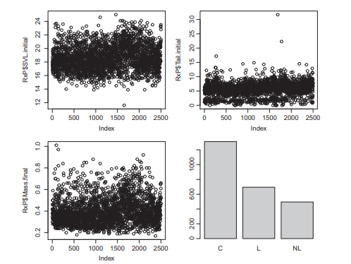
The purpose of this chapter is to expand on what you learned in Chapter 5 , introducing you to the multitude of linear models you can do in $R$. This chapter assumes you are using the RxP.byTank dataset that was created in Chapter $5 .$
This chapter will cover the following topics:

Analysis of Variance (ANOVA) with more than one predictor
Linear regression
Analysis of Covariance (ANCOVA)
Plotting regressions
Predicting values from a model
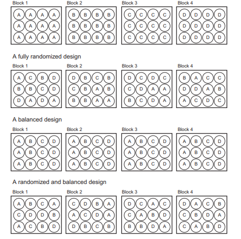
As a reminder, we are only concerned only with “normal” data for the moment. By normal data, we are referring to data that fit a normal distribution, with an approximately even distribution of values around the mean. Table $6.1$ shows the variety of models that we can conduct under the $\operatorname{lm}()$ framework. Note that all we do is change the number and type of predictor variables to do different types of models.

统计代写|应用统计代写applied statistics代考|GETTING STARTED

The model commonly referred to as a linear model, or $\operatorname{lm}()$, is one of the most flexible and useful in all of statistics. We will discuss generalized linear models (GLMs) in Chapter 7 , which allow us to analyze non-normally distributed data. Before we get started, let’s load all the packages you will need here. This is something I like to do at the head of any script file. Remember that if you don’t have one of these packages already, you can download it by using the Package Installer menu, or simply by typing install.packages() at the prompt and put the name of the package in quotes inside the parentheses. If you use the menu, make sure you click the button to “include dependencies.” This is important since most packages rely on other packages to run.

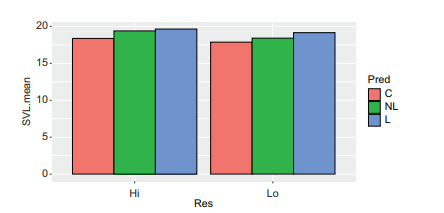
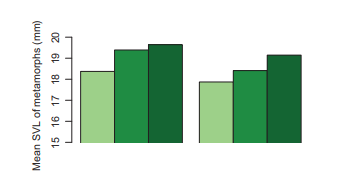
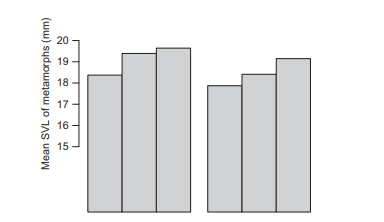
This shows that we have very strong effects of both resource and predator treatments and a significant interaction between the two (albeit not a particularly strong one). In other words, predators alter the age at metamorphosis and so do the different resource levels. However, more importantly our model says that the effect of resources on age at metamorphosis depends on the presence of predators. We could also reframe this in the other direction; the effect of predators on age at metamorphosis depends on the amount of food tadpoles are fed.

统计代写|应用统计代写applied statistics代考|MULTI-WAY ANALYSIS OF VARIANCE-ANOVA

The linear model we ran Chapter 5 (remember, it was called “lm1”) had a single categorical predictor. This type of model is called a one-way Analysis of Variance (ANOVA). But what about when we have multiple categorical predictors that may interact with one another? This is generally referred to as a multi-way ANOVA-a model with two predictors would be a two-way ANOVA, three predictors would be a three-way ANOVA, and so on. Okay, but what does it mean to “interact?”

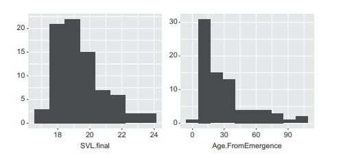
For the RxP data, it is very reasonable to expect that the effects of predators on age at metamorphosis or mass at metamorphosis (or any other response variable) might differ under different resource conditions. To code an interaction between two effects in R you use a colon (:). However, $R$ also provides us with a shortcut for writing both individual effects (e.g., Res or Pred) and the interaction between them (e.g., Res:Pred). Using the asterisk ( $\left.{ }^{}\right)$ tells $\mathrm{R}$ to look at both individual and interaction effects between whatever predictors you have provided. Thus, “Res Pred” is the same as writing “Res+Pred+Res:Pred.” This model is therefore looking at the effects of just resources, of just predators, and then of a possible interaction between the two. Here, we will switch from using Age.FromEmergence

(which is what we examined in Chapter 5) to Age.DPO, which is more intuitive since it tells us the age when froglets metamorphosed in terms of when they were laid as eggs.

Let’s begin with a two-way ANOVA examining the interacting effects of resources and predators on the log-transformed age at metamorphosis.

应用统计代写

统计代写|应用统计代写applied statistics代考|More Linear Models

本章的目的是扩展您在第 5 章中学到的知识，向您介绍可以在其中进行的大量线性模型。R. 本章假设您使用的是在本章中创建的 RxP.byTank 数据集5.
本章将涵盖以下主题：

具有多个预测变量的方差分析 (ANOVA)
线性回归
协方差分析 (ANCOVA)
绘制回归
从模型中预测值
提醒一下，我们目前只关心“正常”数据。通过正态数据，我们指的是符合正态分布的数据，其值在均值附近分布大致均匀。桌子6.1显示了我们可以在流明⁡()框架。请注意，我们所做的只是更改预测变量的数量和类型以执行不同类型的模型。

统计代写|应用统计代写applied statistics代考|GETTING STARTED

该模型通常称为线性模型，或流明⁡(), 是所有统计数据中最灵活和最有用的一种。我们将在第 7 章讨论广义线性模型（GLM），它允许我们分析非正态分布的数据。在我们开始之前，让我们在这里加载您需要的所有包。这是我喜欢在任何脚本文件的开头做的事情。请记住，如果您还没有这些软件包之一，您可以使用 Package Installer 菜单下载它，或者只需在提示符下键入 install.packages() 并将软件包名称放在括号内的引号中。如果您使用菜单，请确保单击“包含依赖项”按钮。这很重要，因为大多数包都依赖其他包来运行。

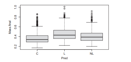
这表明我们对资源和捕食者处理都有非常强的影响，并且两者之间存在显着的相互作用（尽管不是特别强）。换句话说，掠食者改变了变态的年龄，不同的资源水平也是如此。然而，更重要的是，我们的模型表明资源对变态年龄的影响取决于捕食者的存在。我们也可以从另一个方向重新构建它；捕食者对变态年龄的影响取决于喂食蝌蚪的数量。

统计代写|应用统计代写applied statistics代考|MULTI-WAY ANALYSIS OF VARIANCE-ANOVA

我们在第 5 章运行的线性模型（记住，它被称为“lm1”）只有一个分类预测器。这种类型的模型称为方差分析 (ANOVA)。但是，当我们有多个可能相互影响的分类预测变量时呢？这通常被称为多因素方差分析——具有两个预测变量的模型将是双向方差分析，三个预测变量将是三因素方差分析，依此类推。好的，但是“交互”是什么意思？

对于 RxP 数据，可以非常合理地预期捕食者对变态年龄或变态质量（或任何其他响应变量）的影响在不同的资源条件下可能会有所不同。要在 R 中对两个效果之间的交互进行编码，请使用冒号 (:)。然而，R还为我们提供了编写单个效果（例如，Res 或 Pred）和它们之间的交互（例如，Res:Pred）的快捷方式。使用星号 ()告诉R查看您提供的任何预测变量之间的个体效应和交互效应。因此，“Res Pred”与写作“Res+Pred+Res:Pred”相同。因此，该模型正在研究仅资源、捕食者的影响，然后是两者之间可能的相互作用。在这里，我们将从使用 Age.FromEmergence 切换

（这是我们在第 5 章中研究过的）到 Age.DPO，它更直观，因为它告诉我们小蛙从产卵时变态的年龄。

让我们从一个双向方差分析开始，检查资源和捕食者对变态时对数转换年龄的相互作用影响。

统计代写|应用统计代写applied statistics代考请认准statistics-lab™

统计代写请认准statistics-lab™. statistics-lab™为您的留学生涯保驾护航。

金融工程代写

金融工程是使用数学技术来解决金融问题。金融工程使用计算机科学、统计学、经济学和应用数学领域的工具和知识来解决当前的金融问题，以及设计新的和创新的金融产品。

非参数统计代写

非参数统计指的是一种统计方法，其中不假设数据来自于由少数参数决定的规定模型；这种模型的例子包括正态分布模型和线性回归模型。

广义线性模型代考

广义线性模型（GLM）归属统计学领域，是一种应用灵活的线性回归模型。该模型允许因变量的偏差分布有除了正态分布之外的其它分布。

术语广义线性模型（GLM）通常是指给定连续和/或分类预测因素的连续响应变量的常规线性回归模型。它包括多元线性回归，以及方差分析和方差分析（仅含固定效应）。

有限元方法代写

有限元方法（FEM）是一种流行的方法，用于数值解决工程和数学建模中出现的微分方程。典型的问题领域包括结构分析、传热、流体流动、质量运输和电磁势等传统领域。

有限元是一种通用的数值方法，用于解决两个或三个空间变量的偏微分方程（即一些边界值问题）。为了解决一个问题，有限元将一个大系统细分为更小、更简单的部分，称为有限元。这是通过在空间维度上的特定空间离散化来实现的，它是通过构建对象的网格来实现的：用于求解的数值域，它有有限数量的点。边界值问题的有限元方法表述最终导致一个代数方程组。该方法在域上对未知函数进行逼近。[1] 然后将模拟这些有限元的简单方程组合成一个更大的方程系统，以模拟整个问题。然后，有限元通过变化微积分使相关的误差函数最小化来逼近一个解决方案。

tatistics-lab作为专业的留学生服务机构，多年来已为美国、英国、加拿大、澳洲等留学热门地的学生提供专业的学术服务，包括但不限于Essay代写，Assignment代写，Dissertation代写，Report代写，小组作业代写，Proposal代写，Paper代写，Presentation代写，计算机作业代写，论文修改和润色，网课代做，exam代考等等。写作范围涵盖高中，本科，研究生等海外留学全阶段，辐射金融，经济学，会计学，审计学，管理学等全球99%专业科目。写作团队既有专业英语母语作者，也有海外名校硕博留学生，每位写作老师都拥有过硬的语言能力，专业的学科背景和学术写作经验。我们承诺100%原创，100%专业，100%准时，100%满意。

随机分析代写

随机微积分是数学的一个分支，对随机过程进行操作。它允许为随机过程的积分定义一个关于随机过程的一致的积分理论。这个领域是由日本数学家伊藤清在第二次世界大战期间创建并开始的。

时间序列分析代写

随机过程，是依赖于参数的一组随机变量的全体，参数通常是时间。随机变量是随机现象的数量表现，其时间序列是一组按照时间发生先后顺序进行排列的数据点序列。通常一组时间序列的时间间隔为一恒定值（如1秒，5分钟，12小时，7天，1年），因此时间序列可以作为离散时间数据进行分析处理。研究时间序列数据的意义在于现实中，往往需要研究某个事物其随时间发展变化的规律。这就需要通过研究该事物过去发展的历史记录，以得到其自身发展的规律。

回归分析代写

多元回归分析渐进（Multiple Regression Analysis Asymptotics）属于计量经济学领域，主要是一种数学上的统计分析方法，可以分析复杂情况下各影响因素的数学关系，在自然科学、社会和经济学等多个领域内应用广泛。

MATLAB代写

MATLAB 是一种用于技术计算的高性能语言。它将计算、可视化和编程集成在一个易于使用的环境中，其中问题和解决方案以熟悉的数学符号表示。典型用途包括：数学和计算算法开发建模、仿真和原型制作数据分析、探索和可视化科学和工程图形应用程序开发，包括图形用户界面构建MATLAB 是一个交互式系统，其基本数据元素是一个不需要维度的数组。这使您可以解决许多技术计算问题，尤其是那些具有矩阵和向量公式的问题，而只需用 C 或 Fortran 等标量非交互式语言编写程序所需的时间的一小部分。MATLAB 名称代表矩阵实验室。MATLAB 最初的编写目的是提供对由 LINPACK 和 EISPACK 项目开发的矩阵软件的轻松访问，这两个项目共同代表了矩阵计算软件的最新技术。MATLAB 经过多年的发展，得到了许多用户的投入。在大学环境中，它是数学、工程和科学入门和高级课程的标准教学工具。在工业领域，MATLAB 是高效研究、开发和分析的首选工具。MATLAB 具有一系列称为工具箱的特定于应用程序的解决方案。对于大多数 MATLAB 用户来说非常重要，工具箱允许您学习和应用专业技术。工具箱是 MATLAB 函数（M 文件）的综合集合，可扩展 MATLAB 环境以解决特定类别的问题。可用工具箱的领域包括信号处理、控制系统、神经网络、模糊逻辑、小波、仿真等。

R语言代写	问卷设计与分析代写
PYTHON代写	回归分析与线性模型代写
MATLAB代写	方差分析与试验设计代写
STATA代写	机器学习/统计学习代写
SPSS代写	计量经济学代写
EVIEWS代写	时间序列分析代写
EXCEL代写	深度学习代写
SQL代写	各种数据建模与可视化代写

统计代写|应用统计代写applied statistics代考|Basic Statistical Analyses using R

Posted on 2022年5月16日2022年5月16日 by statistics-lab

如果你也在怎样代写应用统计applied statistics这个学科遇到相关的难题，请随时右上角联系我们的24/7代写客服。

我们提供的应用统计applied statistics及其相关学科的代写，服务范围广, 其中包括但不限于:

Statistical Inference 统计推断
Statistical Computing 统计计算
Advanced Probability Theory 高等概率论
Advanced Mathematical Statistics 高等数理统计学
(Generalized) Linear Models 广义线性模型
Statistical Machine Learning 统计机器学习
Longitudinal Data Analysis 纵向数据分析
Foundations of Data Science 数据科学基础

统计代写|应用统计代写applied statistics代考|Basic Statistical Analyses using R

The purpose of this chapter is to introduce you to some basic statistical analyses using $R$. This chapter assumes you are using the RxP.clean dataset that was created in the Chapter 3 .
We will cover the following topics:

Assessing data normality
Some basic non-parametric statistics
Student’s t-test
One-way Analysis of Variance (ANOVA)
We have now seen how to use a function like qplot() to look at your data in various ways. For example, you can plot a histogram of your response variable and see how it is distributed. However, as you move beyond the initial steps of data exploration and start to think about data analysis, there are several questions you should ask yourself. The most important of which is just what kind of data do you have?

This might seem like a simple question at first, but it is paramount for determining the analyses you will conduct. When we talk about data, are we talking about your response or your predictor variables? The answer is both of course. Knowing the shape of your response and predictor variables will determine what sort of analysis you do. In addition to simply knowing if the data are normal or not, you should be mindful of if you have one predictor or multiple predictors, and if your predictors are continuous (a bunch of numbers) or discrete (different categories). For this chapter and the next, we will just concern ourselves with analyzing data where the response variable is normally distributed.

统计代写|应用统计代写applied statistics代考|AVOIDING PSEUDOREPLICATION

Although we have data on nearly 2500 individual metamorphs, those data are not all independent from one another. This is because groups of tadpoles were raised in common environments (the mesocosms, aka tanks) and variation between tanks may make certain individuals more similar than others. If we treat all individuals as independent, we are committing pseudoreplication, which is when you artificially inflate your sample size of independent observations. This was first mentioned in Chapter 2 , but for more details, see the classic article Hurlbert, S.H. 1984. “Pseudoreplication and the design of ecological field experiments.” Ecological Monographs $54(2): 187-211$. It’s a little long, but it’s a great read!

One easy way to avoid pseudoreplication is to utilize the mean value for each tank instead of that of individuals. We can summarize our entire dataset with relative ease using the summarize() function that was introduced in Chapter 3. We will have to get rid of column 1 on Individual ID and column 3 which shows the tank within each block because those would not be meaningful to average at the tank level. Recall that in order to use summarize() we first: 1) define our dataset, then 2) define the different variables we want to group our data by with the group_by() function, and lastly 3) use summarize() to create the variables that are the mean values from the raw dataset. At each of the three steps you pipe your data from one line to the next. You could also use the aggregate() function by defining the 7 columns to summarize (our response variables) and binding them together in a single object using the function cbind(), which binds two or more columns together, then give it the various predictor variables we want to use to summarize the data. Here, we will use summarize(), which just makes more sense. Recall that these functions are found in the dplyr package.

One other thing to notice in the following code is that there are more variables than necessary in the group_by() function. All we need to uniquely identify each tank is the variable “Tank.Unique” or the three treatments in combination. Including all of them, as well as the “Block” variable, we will merely carry more columns through to our new summarized dataset. Lastly, notice that we are storing the output of this set of code as a new object called “RxP.byTank.”

统计代写|应用统计代写applied statistics代考|Looking at the data

The first and easiest thing to do if you want to see if your data are normal or not is to plot the histogram of values. You could use either the hist() function or the $q$ plot() function found in the ggplot2 package. Either way, a histogram should give you a general sense of what your data look like. Remember that data which are normally distributed will have a relatively even spread of values above and below the mean, like that shown in Figure 5.1. Let’s look at the variables “Age.FromEmergence” and “SVL.final” and plot them using qplot() from the ggplot2 package. Remember, you have to load the package first using the library() function. Notice in the following code that we can use the “bins=” argument to specify how fine we want the histogram to break up the data. Also notice I’ve loaded the package cowplot which contains the function plot_grid() which allows us to plot multiple different figures together in a single window.

Looking at these two histograms (Figure $5.2$ ) is quite informative. The SVL data appear almost normal, although the data have a slight tail to the right. The Age data are, however, very skewed; most individuals emerged very early in the period of metamorphosis, but the tail is very long with individuals still emerging from tanks more than 100 days after the first metamorphs. Many biological patterns can be made normal with logtransformation, so a good first step is to see what effect that has on our data. Data that can be made normal upon log-transformation are referred to as “lognormal.” As we explored in Chapter 3, plotting data as a density plot can also be useful, and so both will now be shown in Figure 5.3.

应用统计代写

统计代写|应用统计代写applied statistics代考|Basic Statistical Analyses using R

本章的目的是向您介绍一些基本的统计分析，使用R. 本章假设您使用的是在第 3 章中创建的 RxP.clean 数据集。
我们将涵盖以下主题：

评估数据正态性
一些基本的非参数统计
学生 t 检验
单因素方差分析 (ANOVA)
我们现在已经了解了如何使用 qplot() 之类的函数以各种方式查看数据。例如，您可以绘制响应变量的直方图并查看其分布情况。但是，当您超越数据探索的初始步骤并开始考虑数据分析时，您应该问自己几个问题。其中最重要的是您拥有什么样的数据？

乍一看，这似乎是一个简单的问题，但它对于确定您将进行的分析至关重要。当我们谈论数据时，我们是在谈论您的反应还是您的预测变量？答案当然是两者。了解响应变量和预测变量的形状将决定您进行何种分析。除了简单地知道数据是否正常之外，您还应该注意您是否有一个或多个预测变量，以及您的预测变量是连续的（一堆数字）还是离散的（不同的类别）。对于本章和下一章，我们将只关注分析响应变量正态分布的数据。

统计代写|应用统计代写applied statistics代考|AVOIDING PSEUDOREPLICATION

尽管我们拥有近 2500 个单独变质的数据，但这些数据并非都相互独立。这是因为蝌蚪群是在普通环境（中宇宙，又名坦克）中饲养的，而坦克之间的差异可能会使某些个体比其他个体更相似。如果我们将所有个体视为独立个体，我们就是在进行伪复制，即人为地夸大独立观察的样本量。这在第 2 章中首次提到，但更多详细信息，请参阅经典文章 Hurlbert, SH 1984。“Pseudoreplication and the design of eco field Experiments”。生态专着54(2):187−211. 有点长，但是读起来很不错！

避免伪复制的一种简单方法是利用每个坦克的平均值而不是个体的平均值。我们可以使用第 3 章中介绍的 summarise() 函数相对轻松地总结我们的整个数据集。我们将不得不去掉关于个人 ID 的第 1 列和显示每个块内的坦克的第 3 列，因为这些没有意义平均在油箱液位。回想一下，为了使用 summarise()，我们首先：1) 定义我们的数据集，然后 2) 使用 group_by() 函数定义我们想要分组数据的不同变量，最后 3) 使用 summarise() 创建来自原始数据集的平均值的变量。在这三个步骤中的每一个步骤中，您都将数据从一行传输到下一行。您还可以通过定义 7 列来汇总（我们的响应变量）并使用函数 cbind() 将它们绑定到单个对象中来使用 aggregate() 函数，该函数将两个或更多列绑定在一起，然后给它各种预测器我们想用来总结数据的变量。在这里，我们将使用 summarise()，这更有意义。回想一下，这些函数可以在 dplyr 包中找到。

在下面的代码中要注意的另一件事是 group_by() 函数中的变量多于必要的变量。我们需要唯一标识每个坦克的是变量“Tank.Unique”或三种处理的组合。包括所有这些，以及“块”变量，我们只会将更多列带到我们的新汇总数据集中。最后，请注意我们将这组代码的输出存储为一个名为“RxP.byTank”的新对象。

统计代写|应用统计代写applied statistics代考|Looking at the data

如果您想查看您的数据是否正常，首先也是最简单的事情是绘制值的直方图。您可以使用 hist() 函数或qggplot2 包中的 plot() 函数。无论哪种方式，直方图都应该让您大致了解数据的外观。请记住，正态分布的数据在平均值上方和下方的值分布相对均匀，如图 5.1 所示。让我们看一下变量“Age.FromEmergence”和“SVL.final”，并使用 ggplot2 包中的 qplot() 绘制它们。请记住，您必须首先使用 library() 函数加载包。请注意，在下面的代码中，我们可以使用“bins=”参数来指定我们希望直方图分解数据的精细程度。还要注意我已经加载了包含函数 plot_grid() 的包cowplot，它允许我们在一个窗口中一起绘制多个不同的图形。

查看这两个直方图（图5.2) 信息量很大。SVL 数据看起来几乎正常，尽管数据向右有轻微的尾部。然而，年龄数据非常倾斜；大多数个体在变态期很早就出现了，但尾巴很长，在第一次变态后 100 多天后个体仍然从坦克中出现。许多生物模式可以通过对数转换变得正常，所以第一步是看看它对我们的数据有什么影响。在对数转换后可以正常化的数据称为“对数正态”。正如我们在第 3 章中所探讨的，将数据绘制为密度图也很有用，因此现在两者都将显示在图 5.3 中。

统计代写请认准statistics-lab™. statistics-lab™为您的留学生涯保驾护航。

金融工程代写

非参数统计代写

非参数统计指的是一种统计方法，其中不假设数据来自于由少数参数决定的规定模型；这种模型的例子包括正态分布模型和线性回归模型。

广义线性模型代考

广义线性模型（GLM）归属统计学领域，是一种应用灵活的线性回归模型。该模型允许因变量的偏差分布有除了正态分布之外的其它分布。

有限元方法代写

随机分析代写

时间序列分析代写

回归分析代写

MATLAB代写

R语言代写	问卷设计与分析代写
PYTHON代写	回归分析与线性模型代写
MATLAB代写	方差分析与试验设计代写
STATA代写	机器学习/统计学习代写
SPSS代写	计量经济学代写
EVIEWS代写	时间序列分析代写
EXCEL代写	深度学习代写
SQL代写	各种数据建模与可视化代写

统计代写|应用统计代写applied statistics代考|Histograms and density plots

Posted on 2022年5月16日2022年5月16日 by statistics-lab

如果你也在怎样代写应用统计applied statistics这个学科遇到相关的难题，请随时右上角联系我们的24/7代写客服。

我们提供的应用统计applied statistics及其相关学科的代写，服务范围广, 其中包括但不限于:

Statistical Inference 统计推断
Statistical Computing 统计计算
Advanced Probability Theory 高等概率论
Advanced Mathematical Statistics 高等数理统计学
(Generalized) Linear Models 广义线性模型
Statistical Machine Learning 统计机器学习
Longitudinal Data Analysis 纵向数据分析
Foundations of Data Science 数据科学基础

统计代写|应用统计代写applied statistics代考|Histograms and density plots

By default, if you plot just a single continuous variable using $q$ plot( $), R$ will plot a histogram (Figure 4.5, left). Histograms are extremely useful for seeing the distribution of your data. Do they look normally distributed? Are they skewed to one side or the other? There is technically no need to specify a “geom” here, but I think it is a good idea to be clear in your code, so I would recommend it.
Make a basic histogram
ac-qplot (data=Rxp. clean
$\mathrm{x}=$ Mass . final,
geom $=$ “histogram”)
The same principle of using the color or fill arguments as a way to view your data apply to histograms, but with one caveat. If you add a fill or color argument to a histogram in qplot ()$, \mathrm{R}$ will make a stacked histogram (Figure 4.5, middle). It can be more useful to see the data distributions overlayed on one another. This is best achieved with a density plot, which is similar to a histogram but instead plots a smoothed line that shows the shape of the data (Figure 4.5, right). Note that you should use the “col” argument in the density plot instead of the “fill” argument. What happens if you do not?
Hake a stacked histogram
be-qplot (data=RxP. clean,
$x=$ Mass.final,
geom=”histogram”,

Make a stacked histogram,

be-qplot (data=RxP.clean,
x=Mass. final,
geom= “histogram”,
fill=Pred)

Make overlayed density plots

ce-qplot (data=RxP. clean,
x=Mass.final,
geom=”density”,
fill=Pred)
#Make overlayed density plots
ce-qplot (data=RxP. clean,
$x=$ Mass. final,
geoms “density”,

统计代写|应用统计代写applied statistics代考|Scatterplots

The same principle works for continuous response variables. Previously, we defined our $\mathrm{x}$-axis as a categorical variable, but if we instead use a continuous variable $\mathrm{R}$ will plot a scatterplot. We can still use facets or colors to visualize the variation in our data, which is extremely useful. For example, in the following code I’ve filled the points based on the resource treatment, and faceted the data based on the predator treatment. Imagine the possibilities (Figure 4.6)!
Hake a serles of scatter plots
qplot (data=RxP. clean,
$x=\log$ (SVL. final),

Make a series of scatter

qplot (data=RxP. clean,
$\mathrm{x}=\log ($ SvL. final),
$\mathrm{y}=\log$ (Mass. final),
col=Res,
facets=. – Pred)
$y=\log ($ Mass. final),
col=Res,
facets=.-Pred)

Note that when we make a plot like this, many of the points end up on top of one another, making it difficult to see all the data. We can add an argument to set the alpha level, or the degree of translucency of the points to alleviate this issue. This is also particularly useful with density plots. For example, we can remake the density plots from above, but this time we will fill them instead of color them and set the alpha to be $0.5$ (Figure $4.7$ ).
qplot (data=RxP. clean,
$x=$ Mass . final,
geom=” density”,
fill=pred,
alpha $=0.5$ )
Note that setting the alpha level in qplot() makes the alpha level $50 \%$ transparent, no matter what value you enter. I will show you how to set it to whatever you want later.

In addition to visualizing our data by setting the fill or color to one of our variables, we can also change the shape of the points based on a variable in our data frame with the “shape $=$ ” argument (Figure 4.8).
Hake a series of scatter plots
qplot (data =kxp. clean,

Mke a series of scatter plots

qplot (data=RxP. clean,
x=log(SVL. final).
$x=\log$ (SVL. final),

统计代写|应用统计代写applied statistics代考|PLOTTING YOUR DATA

In Chapter 3, we saw how to use functions from the dplyr package to summarize our data and we produced a tibble called RP.means that contained the means and standard errors for SVL.initial for each combination of resource and predator treatments. Now, we will see how to take those summarized data and turn them into a nice looking figure. In particular, we are going to make a bar graph. Why a bar graph you ask? There are several reasons really. First, despite their ubiquity in publications, the R gurus do not like bar graphs (or barplots, as we will call them) and making one is kind of a pain in $\mathrm{R}$. This is because bar graphs have an ability to hide a lot about your data (they just show the mean and whatever your error bar of choice is). But the fact that they are difficult to create makes them an excellent tool for teaching many of the ways you can, and probably should, customize your figures. That said, box plots are much more informative and are finally becoming increasingly used in published science. The second reason is that despite their downsides many people still like bar graphs and want to make them, so it is useful to know how to make one.

The most basic function to make a bar graph is barplot(). There are many, many arguments that can be passed to barplot(), which can be viewed in the help file (remember how to get to the help: ?barplot). A slightly improved version is the function barplot2(), which makes plotting error bars much simpler. barplot2() is found in the gplots package. You can also make a barplot in ggplot2. We will go through both examples. I find it useful and instructive to demonstrate the older technique using base graphics first, as it demonstrates how you can modify every little thing in a figure in R. Much of the coding techniques are also useful in ggplot2, and we will use ggplot2 for most everything in this book. If you feel confident

you will never, ever, ever use base graphics, feel free to skip ahead a few pages to the section on ggplot2. However, if you want to learn a little more about $\mathrm{R}$ and customizing figures, I encourage you to follow along with the next few pages of commands.
4.3.1 Making a barplot in base graphics
Let’s start by simply plotting the bars in their most basic form. Note that I am assuming you still have the RPmeans object we created in Chapter $3 .$

应用统计代写

统计代写|应用统计代写applied statistics代考|Histograms and density plots

默认情况下，如果您只绘制一个连续变量，使用q阴谋（),R将绘制一个直方图（图 4.5，左）。直方图对于查看数据的分布非常有用。它们看起来是正态分布的吗？他们偏向一侧还是另一侧？从技术上讲，这里不需要指定“geom”，但我认为在你的代码中清晰是个好主意，所以我会推荐它。
制作基本直方图
ac-qplot (data=Rxp.clean
X=大量的。最后，
几何=“直方图”）
使用颜色或填充参数作为查看数据的方式的相同原则适用于直方图，但有一个警告。如果在 qplot() 中为直方图添加填充或颜色参数,R将制作一个堆叠直方图（图 4.5，中间）。查看相互叠加的数据分布可能更有用。最好使用密度图来实现这一点，它类似于直方图，而是绘制一条显示数据形状的平滑线（图 4.5，右）。请注意，您应该在密度图中使用“col”参数而不是“fill”参数。如果不这样做会怎样？
绘制堆叠直方图
be-qplot (data=RxP.clean,
X=Mass.final,
geom=”histogram”,

制作堆叠直方图，

be-qplot（数据=RxP.clean，
x=Mass.final，
geom=“直方图”，
填充=Pred）

制作叠加密度图

ce-qplot (data=RxP. clean,
x=Mass.final,
geom=”density”,
fill=Pred) #制作
叠加密度图
ce-qplot (data=RxP. clean,
X=质量最终，
几何“密度”，

统计代写|应用统计代写applied statistics代考|Scatterplots

同样的原理也适用于连续响应变量。之前，我们定义了我们的X-axis 作为分类变量，但如果我们改为使用连续变量R将绘制散点图。我们仍然可以使用构面或颜色来可视化数据的变化，这非常有用。例如，在下面的代码中，我根据资源处理填充了点，并根据捕食者处理对数据进行了分面。想象一下可能性（图 4.6）！
获得一系列散点图
qplot (data=RxP.clean,
X=日志（SVL。最终），

制作一系列散点图

qplot（数据=RxP。干净，
X=日志⁡(SVL。最终的），
是=日志（质量。最终），
col=Res，
facets=。– 预测）
是=日志⁡(Mass.final),
col=Res,
facets=.-Pred)

请注意，当我们制作这样的图时，许多点最终会相互重叠，因此很难查看所有数据。我们可以添加一个参数来设置 alpha 级别，或者点的半透明程度来缓解这个问题。这对于密度图也特别有用。例如，我们可以从上面重新制作密度图，但这次我们将填充它们而不是着色它们并将 alpha 设置为0.5（数字4.7）。
qplot（数据=RxP。干净，
X=大量的。最终，
geom=“密度”，
填充=pred，
alpha=0.5)
请注意，在 qplot() 中设置 alpha 级别会使 alpha 级别50%透明，无论您输入什么值。稍后我将向您展示如何将其设置为您想要的任何内容。

除了通过将填充或颜色设置为我们的变量之一来可视化我们的数据之外，我们还可以根据数据框中的变量来更改点的形状，其中“形状=” 论点（图 4.8）。
Hake 一系列散点图
qplot (data =kxp.clean,

制作一系列散点图

qplot（数据=RxP.clean，
x=log（SVL.final）。
X=日志（SVL。最终），

统计代写|应用统计代写applied statistics代考|PLOTTING YOUR DATA

在第 3 章中，我们看到了如何使用 dplyr 包中的函数来总结我们的数据，我们生成了一个名为 RP.means 的 tibble，其中包含 SVL.initial 对于每种资源和捕食者处理组合的均值和标准误差。现在，我们将了解如何获取这些汇总数据并将它们变成一个漂亮的图形。特别是，我们将制作一个条形图。你问为什么是条形图？确实有几个原因。首先，尽管它们在出版物中无处不在，但 R 大师们不喜欢条形图（或我们称之为条形图），制作一个是一种痛苦R. 这是因为条形图能够隐藏很多关于您的数据的能力（它们只显示平均值以及您选择的误差条）。但它们难以创建的事实使它们成为教授许多您可以并且可能应该自定义图形的方法的绝佳工具。也就是说，箱形图的信息量要大得多，并且最终在已发表的科学中越来越多地使用。第二个原因是尽管有缺点，但许多人仍然喜欢条形图并想要制作它们，因此知道如何制作它很有用。

制作条形图最基本的函数是 barplot()。有很多很多参数可以传递给 barplot()，可以在帮助文件中查看（记住如何获得帮助：?barplot）。稍微改进的版本是函数 barplot2()，它使绘制误差线更加简单。barplot2() 位于 gplots 包中。您还可以在 ggplot2 中制作条形图。我们将通过这两个例子。我发现首先使用基础图形演示旧技术很有用且具有启发性，因为它演示了如何修改 R 中图形中的每一个小东西。许多编码技术在 ggplot2 中也很有用，我们将在大多数情况下使用 ggplot2本书中的一切。如果你感到自信

你永远永远不会使用基本图形，请随意跳过几页到 ggplot2 部分。但是，如果您想了解更多关于R和自定义图形，我鼓励您按照接下来的几页命令进行操作。
4.3.1 在基本图形中制作条形图
让我们从简单地以最基本的形式绘制条形图开始。请注意，我假设您仍然拥有我们在第 1 章中创建的 RPmeans 对象3.

统计代写请认准statistics-lab™. statistics-lab™为您的留学生涯保驾护航。

金融工程代写

非参数统计代写

非参数统计指的是一种统计方法，其中不假设数据来自于由少数参数决定的规定模型；这种模型的例子包括正态分布模型和线性回归模型。

广义线性模型代考

广义线性模型（GLM）归属统计学领域，是一种应用灵活的线性回归模型。该模型允许因变量的偏差分布有除了正态分布之外的其它分布。

有限元方法代写

随机分析代写

时间序列分析代写

回归分析代写

MATLAB代写

R语言代写	问卷设计与分析代写
PYTHON代写	回归分析与线性模型代写
MATLAB代写	方差分析与试验设计代写
STATA代写	机器学习/统计学习代写
SPSS代写	计量经济学代写
EVIEWS代写	时间序列分析代写
EXCEL代写	深度学习代写
SQL代写	各种数据建模与可视化代写

统计代写|应用统计代写applied statistics代考|Hex colors

Posted on 2022年5月16日2022年5月16日 by statistics-lab

如果你也在怎样代写应用统计applied statistics这个学科遇到相关的难题，请随时右上角联系我们的24/7代写客服。

我们提供的应用统计applied statistics及其相关学科的代写，服务范围广, 其中包括但不限于:

Statistical Inference 统计推断
Statistical Computing 统计计算
Advanced Probability Theory 高等概率论
Advanced Mathematical Statistics 高等数理统计学
(Generalized) Linear Models 广义线性模型
Statistical Machine Learning 统计机器学习
Longitudinal Data Analysis 纵向数据分析
Foundations of Data Science 数据科学基础

统计代写|应用统计代写applied statistics代考|Hex colors

Technically, R actually stores color in a system called hexadecimal, which defines each color (red, green, or blue) in terms of two values that range from 0-9, then from A-F, giving a total of 16 different values for each character. Thus, since each color is defined in terms of two number/letter combos, each color has 256 different possible values (the same as we see with RGB!!). Although the code for hexadecimal may not be intuitive, it is easy to look up online exactly what the code is for any color you want to use (just do an internet search for something like “RGB to Hex color”). The main advantage of the Hex system over RGB is that it is very compact to specify whatever color you want. In R, the hex color code goes in quotes and is preceded by a #. An additional two characters can be added to define a degree of translucency (aka, the alpha level). For example, the translucent red color defined previously would be as follows.

统计代写|应用统计代写applied statistics代考|DATA EXPLORATION USING ggplot2

In the last chapter, you learned a little bit about how to make fairly simple figures using base graphics, i.e., the graphics functions that are built into the version of R you downloaded from CRAN. One problem with base graphics is that the figures produced are relatively utilitarian and ugly (at least in many people’s view). There is a whole universe of functions and arguments you can use to make them look better, but in their basic version they are kind of boring and ugly. The relatively recently designed package ggplot2 makes it very easy to make nice looking figures. However, the syntax for coding in ggplot2 is a little different than base graphics. There are two workhorse functions in ggplot 2: the first is qplot() (which stands for “quick plot”) and the other is ggplot(). We will cover $g g p l o t()$ at a later date. For now, let’s explore qplot().

统计代写|应用统计代写applied statistics代考|Boxplots

Earlier, you made a boxplot using base graphics. The syntax for this was conveniently the same that we will use to define statistical models (“response $\sim$ predictor”). ggplot2 does things differently. Instead, you explicitly specify what variable you want on the $x$ or $y$ axes, and you specify the type of plot you want using the geom argument, which is short for geometric object. Don’t forget that in order to use the $q$ plot() function you first need to load the ggplot2 library. Also remember that you have to do this each time you restart $R$. In the following code I am using the number sign (#) to annotate the code. When you come back to your analyses in a week, a month, or a year, you need to have notes to remind yourself of what you were doing. Always leave notes in your script file for your future self.

Even in the most basic form, the figure made with ggplot2 (Figure $4.1$ ) is nicer looking (to many people), but this is not why ggplot2 is so useful. Where ggplot2 really shines is in its ability to add colors and to plot data across many different variables at once, as well as to easily take the same type of data and plot it in different ways within a single coding framework. For example, if you want to add colors to your figures, you can use either the “col” or “fill” arguments. In the case of a boxplot, “col” will change the color of the outline of the boxes whereas “fill” changes the color inside each one. The effects of “col” or “fill” will differ based on the particular type of plot you are making. One thing that is really cool about plotting with ggplot2 is that we define the colors as one of the variables in our dataset. R will be able to look at our data frame and know how many categories we have, and therefore how many colors to plot, and will even add a legend for us. So handy！

应用统计代写

统计代写|应用统计代写applied statistics代考|Hex colors

从技术上讲，R 实际上将颜色存储在一个称为十六进制的系统中，该系统将每种颜色（红色、绿色或蓝色）定义为从 0 到 9 的两个值，然后是 AF，每个字符总共有 16 个不同的值. 因此，由于每种颜色都是根据两个数字/字母组合定义的，因此每种颜色都有 256 个不同的可能值（与我们在 RGB 中看到的相同！！）。虽然十六进制的代码可能不直观，但可以很容易地在线查找您想要使用的任何颜色的代码（只需在互联网上搜索“RGB 到十六进制颜色”之类的内容）。Hex 系统相对于 RGB 的主要优势在于它非常紧凑，可以指定您想要的任何颜色。在 R 中，十六进制颜色代码用引号括起来，并以 # 开头。可以添加另外两个字符来定义半透明程度（又名，阿尔法水平）。例如，之前定义的半透明红色如下。

统计代写|应用统计代写applied statistics代考|DATA EXPLORATION USING ggplot2

在上一章中，您学习了一些关于如何使用基本图形（即从 CRAN 下载的 R 版本中内置的图形功能）制作相当简单的图形的知识。基本图形的一个问题是生成的图形相对实用且丑陋（至少在许多人看来）。您可以使用一整套函数和参数来使它们看起来更好，但在它们的基本版本中，它们有点无聊和丑陋。相对最近设计的包 ggplot2 使得制作漂亮的图形变得非常容易。但是，ggplot2 中的编码语法与基本图形略有不同。ggplot 2 中有两个主力函数：第一个是 qplot()（代表“快速绘图”），另一个是 ggplot()。我们将涵盖GGpl这吨()在以后的日期。现在，让我们探索 qplot()。

统计代写|应用统计代写applied statistics代考|Boxplots

之前，您使用基本图形制作了箱线图。其语法方便地与我们将用于定义统计模型的相同（“响应∼预测器”）。ggplot2 做的事情不同。相反，您在X或者是轴，并使用 geom 参数指定所需的绘图类型，它是几何对象的缩写。不要忘记，为了使用q你首先需要加载 ggplot2 库的 plot() 函数。另请记住，每次重新启动时都必须执行此操作R. 在下面的代码中，我使用数字符号 (#) 来注释代码。当你在一周、一个月或一年后回到你的分析中时，你需要做笔记来提醒自己你在做什么。总是在你的脚本文件中为你未来的自己留下笔记。

即使是最基本的形式，用ggplot2制作的图（图4.1) 更好看（对很多人来说），但这并不是 ggplot2 如此有用的原因。ggplot2 真正闪耀的地方在于它能够同时添加颜色和跨多个不同变量绘制数据，以及轻松获取相同类型的数据并在单个编码框架内以不同方式绘制它。例如，如果要为图形添加颜色，可以使用“col”或“fill”参数。在箱线图的情况下，“col”将改变盒子轮廓的颜色，而“fill”改变每个盒子内部的颜色。“col”或“fill”的效果将根据您制作的特定类型的情节而有所不同。使用 ggplot2 绘图非常酷的一件事是，我们将颜色定义为数据集中的变量之一。R 将能够查看我们的数据框并知道我们有多少类别，因此要绘制多少种颜色，甚至会为我们添加一个图例。太方便了！

统计代写请认准statistics-lab™. statistics-lab™为您的留学生涯保驾护航。

金融工程代写

非参数统计代写

非参数统计指的是一种统计方法，其中不假设数据来自于由少数参数决定的规定模型；这种模型的例子包括正态分布模型和线性回归模型。

广义线性模型代考

广义线性模型（GLM）归属统计学领域，是一种应用灵活的线性回归模型。该模型允许因变量的偏差分布有除了正态分布之外的其它分布。

有限元方法代写

随机分析代写

时间序列分析代写

回归分析代写

MATLAB代写

R语言代写	问卷设计与分析代写
PYTHON代写	回归分析与线性模型代写
MATLAB代写	方差分析与试验设计代写
STATA代写	机器学习/统计学习代写
SPSS代写	计量经济学代写
EVIEWS代写	时间序列分析代写
EXCEL代写	深度学习代写
SQL代写	各种数据建模与可视化代写

统计代写|应用统计代写applied statistics代考|SUMMARIZING AND MANIPULATING DATA

Posted on 2022年5月16日2022年5月16日 by statistics-lab

如果你也在怎样代写应用统计applied statistics这个学科遇到相关的难题，请随时右上角联系我们的24/7代写客服。

我们提供的应用统计applied statistics及其相关学科的代写，服务范围广, 其中包括但不限于:

Statistical Inference 统计推断
Statistical Computing 统计计算
Advanced Probability Theory 高等概率论
Advanced Mathematical Statistics 高等数理统计学
(Generalized) Linear Models 广义线性模型
Statistical Machine Learning 统计机器学习
Longitudinal Data Analysis 纵向数据分析
Foundations of Data Science 数据科学基础

统计代写|应用统计代写applied statistics代考|SUMMARIZING AND MANIPULATING DATA

There are many tools in $\mathrm{R}$ to help you summarize your data efficiently. I think there are two functions worth knowing about at this stage: aggregate() from base $\mathrm{R}$ and summarize() from the dplyr package.
aggregate() is a very useful function that takes a column of raw data and summarizes it across one or more groups based on some chosen function (e.g., calculate the mean or the standard deviation, etc.). One nice think about using aggregate() is that you code the function of how you want your data summarized in the exact same format that you use for specifying plots or models (which we will cover in Chapter 5). The output of aggregate() is a data frame, which makes it easy to then use for plotting figures or other purposes. aggregate() takes three arguments: 1) the response and predictor variables, 2) the function you want to execute (with the “FUN=” argument), and 3) the data frame where the data can be found. For example, if you want to calculate the mean size of metamorphs at emergence across all combinations of Food and Resource treatments, you can type the following:

The package $d p l y r$ has many useful functions for data wrangling which we will cover in this book. By using some of these in combination, you can easily summarize your data. The utility of this may not be completely evident now, but it will be later, I promise (particularly in Chapter 9). The downside of dplyr is that, much like ggplot2, it has its own lexicon that is fairly distinct from the rest of $R$, meaning that you have to learn a whole

different set of commands. So be it. It’s pretty great once you learn the coding.

By using a few choice functions, such as group_by() and summarize(), we can easily say we want to calculate the means of whatever variable (or variables) we are interested in. Note of course that you can use different functions besides mean(), which is what we will start with here. The other important thing to note in the following code is the use of the pipe command, ‘ $\%>\%$ ‘, which designates the output of one line to be the input of the next.

统计代写|应用统计代写applied statistics代考|Introduction to Plotting

Before we get into the meat of how to most efficiently plot your data, it is useful to take a moment to talk about what makes a good figure. What is it that makes a high-quality figure, one that is suitable for publication or use in a presentation? I would argue that judicious use of color, large clear text and labels, and efficient usage of plot space are three hallmarks of a good figure. It is often useful to create multiple panels to show different aspects of your data. These fundamentals are the same whether you are making your figures in $R$ or not or using base graphics or ggplot2. If you are interested in a deeper dive into this topic, please check out the excellent book Fundamentals of Data Visualization by Claus O. Wilke, professor at The University of Texas (UT) Austin. He has written a particularly elegant and useful package called cowplot that provides not only a nice and easy to apply theme for ggplot2 to make

your figures look betterm, but it also contains many other functions which are useful.

There are two main ways to make figures in R: base graphics (i.e., those that are built into the base version of $R$ you downloaded from the Comprehensive R Archive Network (https://cran.r-project.org/) (CRAN) and using the package ggplot2. There are functions in other packages (e.g., the scatterplot() function in the car package, or the barplot2() function in the gplots package), but these all utilize the basic coding of base graphics. While ggplot 2 and base graphics use different coding styles, the fundamentals that make an effective graphic remain the same. Both types of coding allow you to build your graphics piece by piece and really give you control over every aspect of the figure.
Let’s talk about some basic nuts and bolts that are useful to know.

统计代写|应用统计代写applied statistics代考|Named colors

R has 657 named colors stored and ready to use. The full list of these can be viewed by typing colors() (or if you prefer, $\operatorname{colours}())$ at the command prompt. Using named colors is nice because you probably have an intuitive sense of what “slate grey” is going to look like, whereas a color defined by its red, green, and blue (RGB) values is less obvious. If you need to know what the exact RGB values of a named color are, simply use the function $\operatorname{col} 2 \mathbf{r g b}()$ and place the name of the color in quotes in the parentheses. For example, “col2rgb (‘yellow’)” would tell you the RGB values for yellow in $\mathrm{R}$.

$R$ allows you to define colors based on their red, green, and blue (RGB) values. This is particularly useful if you have a color scheme you want to match, perhaps for a presentation in MS PowerPoint or Apple Keynote, and thus you can specify the exact RGB color you are looking for (which might have come from that other program). Colors are defined using the rgb() function, which requires 3 arguments (not surprisingly they are the red, green, and blue values) as well as other optional arguments. The default is that all values have a minimum of 0 and a maximum of 1 , but you can set the max value to be 255 if you wish (which is likely how colors are defined in another program of your choosing). Lastly, you can also make an RGB color translucent by adjusting the alpha level (note that alpha is always on the same scale as the RGB values). For example, to set a color that was pure red but was $30 \%$ translucent (or conversely, $70 \%$ opaque), you would type the following.

应用统计代写

统计代写|应用统计代写applied statistics代考|SUMMARIZING AND MANIPULATING DATA

里面有很多工具R帮助您有效地汇总数据。我认为现阶段有两个函数值得了解：来自 base 的 aggregate()R和 dplyr 包中的 summarise()。
aggregate() 是一个非常有用的函数，它采用一列原始数据并根据某些选择的函数（例如，计算平均值或标准差等）将其汇总到一个或多个组中。使用aggregate() 的一个很好的想法是，你可以用你用来指定图或模型的完全相同的格式来编码你希望如何汇总数据的函数（我们将在第5章中介绍）。aggregate() 的输出是一个数据框，这使得它很容易用于绘制图形或其他目的。aggregate() 接受三个参数：1) 响应变量和预测变量，2) 您要执行的函数（使用“FUN=”参数），以及 3) 可以找到数据的数据框。例如，如果您想计算所有食物和资源处理组合中出现时变质的平均大小，

包裹dpl是r有许多有用的数据整理功能，我们将在本书中介绍。通过结合使用其中的一些，您可以轻松地汇总数据。它的用处现在可能并不完全明显，但我保证会在以后（特别是在第 9 章中）。dplyr 的缺点是，很像 ggplot2，它有自己的词典，与其他词典完全不同R, 这意味着你必须学习一个整体

不同的命令集。随它吧。一旦你学会了编码，它就非常棒了。

通过使用一些选择函数，例如 group_by() 和 summarise()，我们可以轻松地说我们想要计算我们感兴趣的任何变量（或多个变量）的均值。当然请注意，除了均值之外，您还可以使用不同的函数()，这是我们将从这里开始的。以下代码中另一个需要注意的重要事项是管道命令的使用，’%>%’，它将一行的输出指定为下一行的输入。

统计代写|应用统计代写applied statistics代考|Introduction to Plotting

在我们深入探讨如何最有效地绘制数据之前，花点时间谈谈什么是好图是很有用的。是什么造就了一个高质量的人物，一个适合出版或在演示文稿中使用的人物？我认为明智地使用颜色、大而清晰的文本和标签，以及有效利用情节空间是一个好人物的三个标志。创建多个面板以显示数据的不同方面通常很有用。无论你是在制作你的数字，这些基本原理都是相同的R或不使用或使用基本图形或ggplot2。如果您有兴趣深入研究该主题，请查看德克萨斯大学 (UT) 奥斯汀分校教授克劳斯·威尔克 (Claus O. Wilke) 所著的《数据可视化基础》(Fundamentals of Data Visualization)。他编写了一个特别优雅和有用的包，叫做cowplot，它不仅为ggplot2提供了一个漂亮且易于应用的主题

您的数字看起来更好，但它还包含许多其他有用的功能。

在 R 中制作图形有两种主要方法：基本图形（即那些内置于R您从综合 R 档案网络 (https://cran.r-project.org/) (CRAN) 下载并使用包 ggplot2。其他包中也有函数（如car包中的scatterplot()函数，gplots包中的barplot2()函数），但这些都利用了基础图形的基本编码。虽然 ggplot 2 和基本图形使用不同的编码风格，但制作有效图形的基本原理保持不变。两种类型的编码都允许您逐个构建图形，并真正让您控制图形的各个方面。
让我们谈谈一些有用的基本螺母和螺栓。

统计代写|应用统计代写applied statistics代考|Named colors

R 存储了 657 种命名颜色，可供使用。可以通过键入 colors() 来查看这些的完整列表（或者，如果您愿意，颜色⁡())在命令提示符下。使用命名颜色很好，因为您可能对“板岩灰色”的外观有直观的感觉，而由其红色、绿色和蓝色 (RGB) 值定义的颜色则不太明显。如果您需要知道命名颜色的确切 RGB 值是什么，只需使用函数山口⁡2rGb()并将颜色的名称放在括号中的引号中。例如，“col2rgb (‘yellow’)”会告诉你黄色的 RGB 值R.

R允许您根据红色、绿色和蓝色 (RGB) 值定义颜色。如果您有想要匹配的配色方案，这可能特别有用，可能用于 MS PowerPoint 或 Apple Keynote 中的演示文稿，因此您可以指定您正在寻找的确切 RGB 颜色（可能来自其他程序）。颜色是使用 rgb() 函数定义的，它需要 3 个参数（毫不奇怪，它们是红色、绿色和蓝色值）以及其他可选参数。默认情况下，所有值的最小值为 0 ，最大值为 1 ，但您可以根据需要将最大值设置为 255（这可能是您选择的另一个程序中定义颜色的方式）。最后，您还可以通过调整 alpha 级别使 RGB 颜色半透明（请注意，alpha 始终与 RGB 值处于相同的比例）。例如，30%半透明（或相反，70%不透明），您将键入以下内容。

统计代写请认准statistics-lab™. statistics-lab™为您的留学生涯保驾护航。

金融工程代写

非参数统计代写

非参数统计指的是一种统计方法，其中不假设数据来自于由少数参数决定的规定模型；这种模型的例子包括正态分布模型和线性回归模型。

广义线性模型代考

广义线性模型（GLM）归属统计学领域，是一种应用灵活的线性回归模型。该模型允许因变量的偏差分布有除了正态分布之外的其它分布。

有限元方法代写

随机分析代写

时间序列分析代写

回归分析代写

MATLAB代写

R语言代写	问卷设计与分析代写
PYTHON代写	回归分析与线性模型代写
MATLAB代写	方差分析与试验设计代写
STATA代写	机器学习/统计学习代写
SPSS代写	计量经济学代写
EVIEWS代写	时间序列分析代写
EXCEL代写	深度学习代写
SQL代写	各种数据建模与可视化代写

统计代写|应用统计代写applied statistics代考|Exploratory Data Analysis and Data Summarization

Posted on 2022年5月16日2022年5月16日 by statistics-lab

如果你也在怎样代写应用统计applied statistics这个学科遇到相关的难题，请随时右上角联系我们的24/7代写客服。

我们提供的应用统计applied statistics及其相关学科的代写，服务范围广, 其中包括但不限于:

Statistical Inference 统计推断
Statistical Computing 统计计算
Advanced Probability Theory 高等概率论
Advanced Mathematical Statistics 高等数理统计学
(Generalized) Linear Models 广义线性模型
Statistical Machine Learning 统计机器学习
Longitudinal Data Analysis 纵向数据分析
Foundations of Data Science 数据科学基础

统计代写|应用统计代写applied statistics代考|Exploratory Data Analysis and Data Summarization

The purpose of this chapter is to introduce you to working with and manipulating data in R, exploring data, and plotting. I strongly believe in learning by doing, so let’s start doing some things so you can start learning!

In this book, we will use data from an experiment I conducted when I was a postdoc at the Smithsonian Tropical Research Institute in Panama in 2010 , and which was published in the journal Ecology in 2013 (https:// www.jstor.org/stable/23436298). The experiment was part of a National Science Foundation (NSF) funded project to Drs. Karen Warkentin (Boston University) and James Vonesh (Virginia Commonwealth University) studying the effects of flexible hatching timing by red-eyed treefrog (Agalychnis callidryas) embryos on interactions with predators and food levels and subsequent phenotype development of tadpoles. In order to follow along with the examples in this chapter, and the rest of the

book, you should download from the Github page for this book (https:// github.com/jtouchon/Applied-Statistics-with-R) a .csv file titled “RxP.csv”” The data are called by the short name “RxP” which stands for “Resourceby-Predation, which was the nature of the experiment (we were studying the interaction of resources and predators). This brings up a chance to reiterate a small but important point: since $\mathrm{R}$ is entirely based on typing commands by hand, you should give your datasets and variables short names so that they are quick and easy to type.
First, let’s get a handle on what the data are.

统计代写|应用统计代写applied statistics代考|READING IN THE DATA FILE

If you are loading a data file from somewhere on your computer, you will read it into the active workspace with the command read.csv(). If your dataset has categorical variables, you will want to include the argument stringsAsFactors= $T$, which tells the function to automatically make any columns that have character data in them factors. If the data are in your working directory, you would simply do the following (and remember, you should be working in a script window!). Note that you have to assign the data to an object. What happens if you do not? What is the working directory you ask? It is the directory that $R$ will look in by default. To find out where $R$ is looking, type getwd( $)$ at the prompt.

You can set your working directory with the function setwd( $)$, where you would put in the parenthesis a path to a folder on your computer. Make sure to put the path in quotes. Some folks like to set a working directory for each project they have. Others prefer to keep the working directly in a single place and just code the path to certain files. Choose whichever works for you. If your data are not in your working directory, you will need to specify exactly where to find the file on your computer.

统计代写|应用统计代写applied statistics代考|DATA EXPLORATION AND ERROR CHECKING

Whenever you start working with a dataset in $\mathrm{R}$, you should first devote substantial time to checking it for errors. Questions you should ask yourself include:

Did the data import correctly?
Are the column names correct?
Are the types of data appropriate? (e.g., factor vs numerical)
Are the numbers of columns and rows appropriate?
Are there typos?
If, for example, a column that is supposed to be numerical shows up as a factor, that likely indicates a typo where you accidentally have text in place of a number (remember, each column in a data frame is a vector, and vectors can only have one mode, so a vector with both numbers and characters is treated as if it is all characters). Similarly, if you have a factor that should have 3 categories, but imports with 4 , you likely have a typo (e.g., “predator” vs “predtaor”), and the misspelled version is showing up as a separate category. These sorts of mistakes are very common!

Because this dataset has been thoroughly examined (very thoroughly!), these types of errors are not present. However, you might want to change the names of columns or remove outliers, which we will cover in the subsequent sections.

应用统计代写

统计代写|应用统计代写applied statistics代考|Exploratory Data Analysis and Data Summarization

本章的目的是向您介绍在 R 中使用和操作数据、探索数据和绘图。我坚信边做边学，所以让我们开始做一些事情，这样你就可以开始学习了！

在本书中，我们将使用我 2010 年在巴拿马史密森热带研究所做博士后时进行的一项实验的数据，该实验于 2013 年发表在《生态学》杂志上（https://www.jstor.org/稳定/23436298）。该实验是美国国家科学基金会 (NSF) 资助的 Drs 项目的一部分。Karen Warkentin（波士顿大学）和 James Vonesh（弗吉尼亚联邦大学）研究红眼树蛙 (Agalychnis callidryas) 胚胎灵活的孵化时间对与捕食者和食物水平的相互作用以及蝌蚪后续表型发育的影响。为了跟随本章中的示例，以及其余的

书，你应该从本书的 Github 页面 (https://github.com/jtouchon/Applied-Statistics-with-R) 下载一个名为“RxP.csv”的 .csv 文件。 “RxP”代表“Resourceby-Predation”，这是实验的本质（我们正在研究资源和捕食者的相互作用）。这带来了一个机会来重申一个小而重要的观点：因为R完全基于手动输入命令，你应该给你的数据集和变量起短名称，这样它们就可以快速轻松地输入。
首先，让我们了解一下数据是什么。

统计代写|应用统计代写applied statistics代考|READING IN THE DATA FILE

如果您从计算机上的某个位置加载数据文件，您将使用命令 read.csv() 将其读入活动工作区。如果您的数据集具有分类变量，您将需要包含参数 stringsAsFactors=吨，它告诉函数自动将任何包含字符数据的列作为因子。如果数据在您的工作目录中，您只需执行以下操作（请记住，您应该在脚本窗口中工作！）。请注意，您必须将数据分配给对象。如果不这样做会怎样？你问的工作目录是什么？它是那个目录R默认情况下会查看。找出在哪里R正在寻找，输入 getwd()在提示下。

您可以使用函数 setwd()，您将在括号中放入计算机上文件夹的路径。确保将路径放在引号中。有些人喜欢为他们拥有的每个项目设置一个工作目录。其他人更喜欢将工作直接保存在一个地方，只对某些文件的路径进行编码。选择适合您的。如果您的数据不在您的工作目录中，您将需要准确指定在计算机上找到该文件的位置。

统计代写|应用统计代写applied statistics代考|DATA EXPLORATION AND ERROR CHECKING

每当您开始使用数据集时R，您应该首先花费大量时间来检查它是否有错误。你应该问自己的问题包括：

数据是否正确导入？
列名是否正确？
数据类型是否合适？（例如，因子与数值）
列数和行数是否合适？
有错别字吗？
例如，如果一个应该是数字的列显示为一个因素，这可能表示您不小心用文本代替数字的错字（请记住，数据框中的每一列都是一个向量，向量可以只有一种模式，因此同时包含数字和字符的向量被视为全部字符）。类似地，如果您有一个应该有 3 个类别的因子，但使用 4 导入，则您可能有拼写错误（例如，“predator”与“predtaor”），并且拼写错误的版本显示为单独的类别。这类错误很常见！

因为这个数据集已经过彻底检查（非常彻底！），所以不存在这些类型的错误。但是，您可能想要更改列的名称或删除异常值，我们将在后续部分中介绍这些内容。

统计代写请认准statistics-lab™. statistics-lab™为您的留学生涯保驾护航。

金融工程代写

非参数统计代写

非参数统计指的是一种统计方法，其中不假设数据来自于由少数参数决定的规定模型；这种模型的例子包括正态分布模型和线性回归模型。

广义线性模型代考

广义线性模型（GLM）归属统计学领域，是一种应用灵活的线性回归模型。该模型允许因变量的偏差分布有除了正态分布之外的其它分布。

有限元方法代写

随机分析代写

时间序列分析代写

回归分析代写

MATLAB代写

R语言代写	问卷设计与分析代写
PYTHON代写	回归分析与线性模型代写
MATLAB代写	方差分析与试验设计代写
STATA代写	机器学习/统计学习代写
SPSS代写	计量经济学代写
EVIEWS代写	时间序列分析代写
EXCEL代写	深度学习代写
SQL代写	各种数据建模与可视化代写

统计代写|应用统计代写applied statistics代考|BEST PRACTICES FOR DATA ANALYSIS

Posted on 2022年5月16日2022年5月16日 by statistics-lab

如果你也在怎样代写应用统计applied statistics这个学科遇到相关的难题，请随时右上角联系我们的24/7代写客服。

我们提供的应用统计applied statistics及其相关学科的代写，服务范围广, 其中包括但不限于:

Statistical Inference 统计推断
Statistical Computing 统计计算
Advanced Probability Theory 高等概率论
Advanced Mathematical Statistics 高等数理统计学
(Generalized) Linear Models 广义线性模型
Statistical Machine Learning 统计机器学习
Longitudinal Data Analysis 纵向数据分析
Foundations of Data Science 数据科学基础

统计代写|应用统计代写applied statistics代考|BEST PRACTICES FOR DATA ANALYSIS

Once you have started analyzing your data, how should you actually go about the process? By that I don’t mean “sit at your computer and type code into $R$,” but what is the best way to think about running your analyses and coming to conclusions about your data?

The most important rule of the road is to have clear hypotheses at the outset of analyzing your data. You ran the experiment (presumably) and so you should have an idea of what questions you are trying to answer. It is important that you do not just try to measure everything under the

sun and then look for possible relationships between your variables. If you measure enough things, you are more likely to find a statistically significant relationship that may or may not be meaningful. This is a process known as $p$-hacking or data dredging. Looking for patterns in your data is certainly an okay thing to do, but you should avoid testing every possible predictor you can imagine in the hope of finding something significant that will make your data more publishable. This is particularly true when you have many possible predictor variables.

A second dubious practice which is to be avoided at all costs is HARKing, which stands for “hypothesizing after the results are known.” HARKing basically goes like this: 1) You start with a hypothesis that you want to test; 2) you test it and find a non-significant effect; 3) while doing your series of analyses you come across some other variable which does have a significant explanatory effect; and 4), you omit your original hypothesis and concoct a new hypothesis which fits the results of the study. Essentially, you are coming up with a prediction after you know the answer. It is certainly important to realize that you might learn something new when you analyze your data. Perhaps the unforeseen result causes you to see a new explanatory relationship which you had not considered before. That’s fine, but it is important to be transparent about your original hypothesis versus the new hypothesis. Moreover, you should not be testing all sorts of predictors that may or may not seem important and then trying to come up with explanatory hypotheses after the fact.

The last piece of advice regarding best practices is dont obsess over statistical significance. It has been said many times, but it bears repeating, that the $0.05$ cutoff that is traditionally used to demarcate “significance” is a completely arbitrary line in the sand. Why isn’t it $0.01$ or $0.10$ ? Obviously, the idea of statistical significance is still an oft-used metric in many fields, and we will certainly talk about significance in this book, but don’t obsess over it. It isn’t the be-all and end-all of your research endeavors, because lots of things affect your ability to detect “significance” beyond the validity of your hypotheses, the magnitude of biological affects you measure, or the strength of your data. The more data you have, the greater your ability to detect very small affects. Similarly, with very little data, you will have a hard time detecting even moderate affects. The more variable your data are from individual to individual, the harder a time you will have detecting significance. So, focus your energy on understanding and estimating the explanatory power of your predictor variables. What you want to know is if there is a relationship between your predictor and response variables and how confident you can be in any relationship you’ve tried to quantify, so try to keep that in your mind at all times while analyzing your data.

统计代写|应用统计代写applied statistics代考|HOW TO DECIDE BETWEEN COMPETING ANALYSES

Something we will explore later in this book with practical, real-world examples is how to choose amongst different possible ways to analyze your data. However, it is still useful to think about this issue up front, because it is an important one. Many times, you will be faced with different possible ways to analyze your data and different methods might have certain pros and cons.

At the end of the day, your job is to pick the statistical analysis that does the best job of representing and interpreting your data. Getting you to the point where you know how to evaluate your data and make that decision is one of the major goals of this book. Sometimes there will be two different types of models that may be essentially equivalent. They may fit equally well, and they may give you very similar answers about the significance of your predictors. Sometimes you might have to choose amongst competing models that give you different answers about the supposed significance (or not) of your predictors. How do you choose which model to go with?

You should be completely neutral about the idea of “significance” and only consider if the model is doing a good job and is appropriate for the data. As we will see in Chapter 7, there are times when you might have a model which might seem appropriate and gives you a highly significant result, but which actually fits very poorly. The opposite can be true as well, where you choose a model that fits poorly and gives you an underwhelming sense of the importance of your predictors. At the end of the day, you need to be able to justify your choice of model to yourself, your reviewers, your supervisors, your colleagues, and anyone else that might look at your analysis. You need to be able to stand behind your decision and explain why you chose one analysis over another. If you can do that, you’ll be in good shape.

统计代写|应用统计代写applied statistics代考|DATA ARE DATA ARE DATA

The data that we will work within this book come from a study I conducted as a postdoc working in the rainforests of Panama at the Smithsonian Tropical Research Institute. I have studied frogs and their eggs and tadpoles since I began my PhD in 2002. I love frogs and their eggs and tadpoles. I think they are the greatest. But, maybe you dont, and maybe you are thinking to yourself: “How do these weird tadpole data relate to me and my analyses? I’m never going to study tadpoles in Panama!” While that might be true, I think that data are data are data, and the spatially nested design of the study we will work through is extremely similar to many other study systems (Figure 2.2).

The shorthand name of the dataset we will work with is “RxP” which stands for “Resource X Predation,” which are the two main things we were manipulating in the study (Chapter 3 will describe the study in more detail). In the RxP dataset, we have individuals that are nested (or grouped, if you will) within tanks, and those tanks are themselves nested within blocks. This is the same as, for example, having multiple mice housed together in a single cage, and then having cages grouped together on different shelves. Or, you might imagine multiple fruit flies measured per vial, and vials are grouped together based on the date they were set up. Similarly, we can think about having multiple genetic strains (i.e., genotypes, families, etc.) that cluster our data into discrete groups. This sort of nested design can also be used to think about repeated measures data, where individuals are measured or sampled repeatedly over time.

Beyond the idea of physically clustered data, we can just think about the tanks as different replicates of an experiment, which is no different from any other experiment. The response variables (also called the “dependent variables”) that were measured during the RxP experiment-things like number of days until metamorphosis or size at metamorphosis-are no different than any other continuous variable that might be measured, be it the length of time a rat freezes after seeing a light flash or the number of pecks a pigeon makes before correctly opening a lever or the number of new leaves produced after adding fertilizer to a growing plant. The predictor variables (also called the “independent variables”) are generally categorical in their nature (i.e., they have several discrete categories), and could easily be replaced by drug treatment or maternal enrichment environment or fertilization regime. As I said earlier, data are data are data. See Figure $2.2$ for a visual depiction of the similarities in data structure.

应用统计代写

统计代写|应用统计代写applied statistics代考|BEST PRACTICES FOR DATA ANALYSIS

一旦你开始分析你的数据，你应该如何实际进行这个过程？我的意思不是“坐在你的电脑前输入代码”R,”但是考虑运行分析并对数据得出结论的最佳方式是什么？

最重要的规则是在分析数据的一开始就有明确的假设。您进行了实验（大概），因此您应该知道您要回答什么问题。重要的是，您不要仅仅尝试在

sun，然后寻找变量之间的可能关系。如果你测量了足够多的东西，你更有可能找到一个可能有意义也可能没有意义的统计显着关系。这是一个被称为p-黑客攻击或数据挖掘。在你的数据中寻找模式当然是一件好事，但你应该避免测试你能想象到的每一个可能的预测变量，以期找到一些重要的东西，让你的数据更容易发布。当您有许多可能的预测变量时尤其如此。

不惜一切代价避免的第二种可疑做法是 HARKing，它代表“知道结果后的假设”。HARKing 基本上是这样的： 1）你从一个你想要检验的假设开始；2）你测试它并发现一个不显着的效果；3）在进行一系列分析时，您会遇到一些其他变量，这些变量确实具有显着的解释效果；4），你省略了你原来的假设，并编造了一个符合研究结果的新假设。从本质上讲，您是在知道答案后提出预测。意识到在分析数据时可能会学到一些新东西，这一点当然很重要。或许意料之外的结果让你看到了一个你以前没有考虑过的新的解释关系。没关系，但重要的是要对您的原始假设与新假设保持透明。此外，您不应该测试所有可能看起来重要或可能不重要的预测变量，然后在事后试图提出解释性假设。

关于最佳实践的最后一条建议是不要沉迷于统计意义。已经说过很多次了，但值得重复的是，0.05传统上用来划分“重要性”的界限是一条完全任意的线。为什么不是0.01或者0.10? 显然，统计显着性的概念仍然是许多领域中经常使用的度量标准，我们肯定会在本书中讨论显着性，但不要太执着于它。这不是您研究工作的全部和最终目的，因为很多事情都会影响您检测“重要性”的能力，超出了假设的有效性、您测量的生物学影响的大小或数据的强度. 您拥有的数据越多，您检测非常小的影响的能力就越大。同样，如果数据很少，即使是中等影响也很难检测到。您的数据在个体之间的差异越大，您就越难发现重要性。因此，将精力集中在理解和估计预测变量的解释力上。

统计代写|应用统计代写applied statistics代考|HOW TO DECIDE BETWEEN COMPETING ANALYSES

我们将在本书后面通过实际的真实示例探讨如何在不同的可能方法中进行选择来分析您的数据。但是，提前考虑这个问题仍然很有用，因为它是一个重要的问题。很多时候，您将面临分析数据的不同可能方法，不同的方法可能有一定的优缺点。

归根结底，您的工作是选择最能代表和解释数据的统计分析。让你知道如何评估数据并做出决定是本书的主要目标之一。有时会有两种不同类型的模型，它们可能本质上是等效的。它们可能同样适合，并且它们可能会就预测变量的重要性给出非常相似的答案。有时，您可能必须在竞争模型中进行选择，这些模型会给您关于预测变量的假设意义（或不重要）的不同答案。您如何选择要搭配的型号？

您应该对“重要性”的概念完全保持中立，只考虑模型是否做得很好并且适合数据。正如我们将在第 7 章中看到的那样，有时您的模型可能看起来很合适，并且给您提供了非常重要的结果，但实际上它的拟合度很差。反之亦然，您选择的模型拟合不佳，并且对预测变量的重要性没有印象。归根结底，您需要能够向您自己、您的审阅者、您的主管、您的同事以及任何可能查看您的分析的其他人证明您选择模型的合理性。您需要能够支持您的决定并解释为什么您选择一种分析而不是另一种分析。如果你能做到这一点，你的身体就会很好。

统计代写|应用统计代写applied statistics代考|DATA ARE DATA ARE DATA

我们将在本书中使用的数据来自我作为博士后在史密森尼热带研究所的巴拿马热带雨林中进行的一项研究。自 2002 年开始攻读博士学位以来，我一直在研究青蛙及其卵和蝌蚪。我喜欢青蛙及其卵和蝌蚪。我认为他们是最伟大的。但是，也许你不知道，也许你在想：“这些奇怪的蝌蚪数据与我和我的分析有什么关系？我永远不会去巴拿马研究蝌蚪！” 虽然这可能是真的，但我认为数据就是数据就是数据，我们将研究的空间嵌套设计与许多其他研究系统极为相似（图 2.2）。

我们将使用的数据集的简写名称是“RxP”，代表“资源 X 捕食”，这是我们在研究中操作的两个主要内容（第 3 章将更详细地描述该研究）。在 RxP 数据集中，我们将个体嵌套（或分组，如果你愿意的话）在坦克中，而这些坦克本身也嵌套在块中。例如，这与将多只老鼠放在一个笼子里，然后将笼子放在不同的架子上是一样的。或者，您可能会想象每个小瓶测量多个果蝇，并且小瓶根据它们的设置日期分组在一起。同样，我们可以考虑拥有多个遗传品系（即基因型、家族等），将我们的数据聚集到离散的组中。

除了物理聚类数据的想法之外，我们可以将坦克视为实验的不同复制品，这与任何其他实验没有什么不同。在 RxP 实验期间测量的响应变量（也称为“因变量”）——比如变态前的天数或变态时的大小——与任何其他可能测量的连续变量没有什么不同，无论是老鼠看到闪光后冻结的时间或鸽子在正确打开杠杆之前的啄食次数或向生长中的植物添加肥料后产生的新叶子的数量。预测变量（也称为“自变量”）在本质上通常是分类的（即，它们有几个离散的类别），并且可以很容易地被药物治疗或母体富集环境或受精方案所取代。正如我之前所说，数据就是数据。见图2.2用于直观描述数据结构的相似性。

统计代写请认准statistics-lab™. statistics-lab™为您的留学生涯保驾护航。

金融工程代写

非参数统计代写

非参数统计指的是一种统计方法，其中不假设数据来自于由少数参数决定的规定模型；这种模型的例子包括正态分布模型和线性回归模型。

广义线性模型代考

广义线性模型（GLM）归属统计学领域，是一种应用灵活的线性回归模型。该模型允许因变量的偏差分布有除了正态分布之外的其它分布。

有限元方法代写

随机分析代写

时间序列分析代写

回归分析代写

MATLAB代写

R语言代写	问卷设计与分析代写
PYTHON代写	回归分析与线性模型代写
MATLAB代写	方差分析与试验设计代写
STATA代写	机器学习/统计学习代写
SPSS代写	计量经济学代写
EVIEWS代写	时间序列分析代写
EXCEL代写	深度学习代写
SQL代写	各种数据建模与可视化代写

统计代写|应用统计代写applied statistics代考|Before You Begin

Posted on 2022年5月16日2022年5月16日 by statistics-lab

如果你也在怎样代写应用统计applied statistics这个学科遇到相关的难题，请随时右上角联系我们的24/7代写客服。

我们提供的应用统计applied statistics及其相关学科的代写，服务范围广, 其中包括但不限于:

Statistical Inference 统计推断
Statistical Computing 统计计算
Advanced Probability Theory 高等概率论
Advanced Mathematical Statistics 高等数理统计学
(Generalized) Linear Models 广义线性模型
Statistical Machine Learning 统计机器学习
Longitudinal Data Analysis 纵向数据分析
Foundations of Data Science 数据科学基础

A diagram on how to plan your sample size | Download Scientific Diagram — 统计代写|应用统计代写applied statistics代考|Before You Begin

统计代写|应用统计代写applied statistics代考|aka Thoughts on Proper Data Analysis

Before we embark on the journey that is learning $R$ and how to use it to analyze your data and make fantastic figures, it is useful to stop and think a little bit about best practices for data analysis.
$2.2$ BASIC PRINCIPLES OF EXPERIMENTAL DESIGN
If there are three words to remember when thinking about experimental design, they are balance, randomization, and replication. In a nutshell, what you are trying to prevent with these three factors is your data being correlated in some way that is unhelpful to your analysis. You are also trying to ensure that your data are independent from one another and that you have enough data to actually determine if your treatments did anything or not (see Boxes 2.1, 2.2, and 2.3).

Obviously, it is not always possible to control these aspects of your data, particularly if you have observational data (as compared to a controlled experiment which you design and run yourself). But, even in the case of observational studies, these principles are important to keep in mind and consider.

统计代写|应用统计代写applied statistics代考|BLOCKED EXPERIMENTAL DESIGNS

Consider the four experimental setups shown in Figure 2.1. Imagine that we are now testing the effects of four fertilizers on plant growth (labelled A, B, C, and D), each with 12 individuals. The experiment is conducted in four separate “blocks” What is a block? It could be many things. Maybe it is a physical way of setting up the experiment, for example, four shelves in an incubator that contain the experimental units or four rooms that contain the cages our individuals live in. Maybe, due to space or time limitations, only 12 individuals can be tested or measured at a time, and thus the experiment has to be run four separate times. Each of these can be considered a “block” so you can hopefully imagine how this idea relates to your own research. Blocks are only important to consider if there is some systematic difference among them.

In the first example, the four treatments will be perfectly correlated with the four blocks. Thus, if we imagine a significant difference is detected in one treatment, there is no way to know if it is because of the experimental treatment or if there was something else going on in that block (or room, or time point, or whatever you want to imagine that block represents). Once again, this is an example of pseudoreplication because it seems like we have a large sample size but in reality, we have a sample size of $\mathrm{N}=1$ in each of our treatments. Despite growing 48 different plants, this design is unreplicated.
The second example is a fully randomized design, where the four treatments are allocated across the four blocks completely at random. The third example is a fully balanced design, where each of the four treatments is assigned to each block in the same manner. Each of these setups has its own advantages and disadvantages.

The fully randomized design is good, and in theory should lead to the highest degree of replication, with all experimental units being truly independent. In reality it can actually work against the principle of balance, since some treatments might end up overrepresented in some blocks and underrepresented in others (e.g., in Figure 2.1, there are six individuals from treatment B in Block 2, but only one in Block 3). In the extreme, leaving your entire setup to random chance could lead to a horribly unbalanced and biased design, but this would be very rare. In general, fully randomizing your experiment is a very good idea!

统计代写|应用统计代写applied statistics代考|YOU CAN (AND SHOULD) PLAN YOUR ANALYSES BEFORE YOU HAVE THE DATA!

In addition to the aspects of experimental design described previously, the other most important thing to do is to have a clear idea of your predictor and response variables before you even start the experiment. Before you ever put a mouse in a testing box or a seed in growth chamber, you should identify what it is you are going to measure. Hopefully, if you know your study system pretty well or perhaps have some preliminary data, you can estimate what the data are going look like which will allow you to think about and plan for what type of analyses you will do. Maybe that sounds like wishful thinking, but this whole book is about the importance of knowing what your data look like, so don’t worry-you’ll get there!

Sir Ronald Fisher, one of the founders of modern statistics, offered one of the best statements about this issue in $1938 .$ Fisher’s point is that because your experimental design directly effects your data analysis, you should think about your analysis up front when planning the experiment.

应用统计代写

统计代写|应用统计代写applied statistics代考|aka Thoughts on Proper Data Analysis

在我们踏上学习之旅之前R以及如何使用它来分析您的数据并制作出色的数字，停下来思考一下数据分析的最佳实践是很有用的。
2.2实验设计的基本原则
如果在考虑实验设计时要记住三个词，它们是平衡、随机化和复制。简而言之，您试图通过这三个因素来防止您的数据以某种对您的分析无益的方式相关联。您还试图确保您的数据彼此独立，并且您有足够的数据来实际确定您的治疗是否有任何作用（参见方框 2.1、2.2 和 2.3）。

显然，控制数据的这些方面并不总是可能的，特别是如果您有观察数据（与您自己设计和运行的受控实验相比）。但是，即使在观察性研究的情况下，这些原则也很重要，需要牢记和考虑。

统计代写|应用统计代写applied statistics代考|BLOCKED EXPERIMENTAL DESIGNS

考虑图 2.1 中所示的四个实验设置。想象一下，我们现在正在测试四种肥料对植物生长的影响（标记为 A、B、C 和 D），每种有 12 个人。实验在四个独立的“块”中进行什么是块？这可能是很多事情。也许这是一种物理的实验设置方式，例如，一个孵化器中的四个架子包含实验单元，或者四个房间包含我们个人居住的笼子。也许，由于空间或时间的限制，只有 12 个人可以一次测试或测量，因此实验必须单独运行四次。每一个都可以被认为是一个“块”，所以你可以想象这个想法与你自己的研究有什么关系。只有在它们之间存在一些系统差异时，才需要考虑块。

在第一个示例中，四种处理将与四个块完全相关。因此，如果我们想象在一种治疗中检测到显着差异，则无法知道这是因为实验性治疗还是在那个街区（或房间，或时间点，或任何你想想象那个块代表）。再一次，这是一个伪复制的例子，因为看起来我们的样本量很大，但实际上，我们的样本量为ñ=1在我们的每一次治疗中。尽管种植了 48 种不同的植物，但这种设计是不可复制的。
第二个示例是完全随机设计，其中四种处理完全随机分配到四个块中。第三个示例是完全平衡的设计，其中四种处理中的每一种都以相同的方式分配给每个区组。这些设置中的每一个都有其自身的优点和缺点。

完全随机的设计是好的，理论上应该导致最高程度的复制，所有实验单元都是真正独立的。实际上，它实际上可能违反平衡原则，因为某些治疗可能最终在某些区块中代表性过高而在其他区块中代表性不足（例如，在图 2.1 中，在区块 2 中有六个来自治疗 B 的个体，但在区块 3 中只有一个）。在极端情况下，将整个设置留给随机机会可能会导致严重的不平衡和有偏见的设计，但这非常罕见。一般来说，完全随机化你的实验是一个非常好的主意！

统计代写|应用统计代写applied statistics代考|YOU CAN (AND SHOULD) PLAN YOUR ANALYSES BEFORE YOU HAVE THE DATA!

除了前面描述的实验设计方面，另一个最重要的事情是在开始实验之前清楚地了解您的预测变量和响应变量。在将鼠标放入测试盒或将种子放入生长室之前，您应该确定要测量的是什么。希望如果您非常了解您的研究系统或者可能有一些初步数据，您可以估计数据的样子，这将使您能够思考和计划您将进行的分析类型。也许这听起来像是一厢情愿，但整本书都是关于了解您的数据是什么样子的重要性，所以不要担心 – 你会到达那里！

现代统计学的奠基人之一罗纳德·费舍尔爵士（Sir Ronald Fisher）在1938. Fisher 的观点是，因为您的实验设计直接影响您的数据分析，所以您应该在计划实验时预先考虑您的分析。

统计代写请认准statistics-lab™. statistics-lab™为您的留学生涯保驾护航。

金融工程代写

非参数统计代写

非参数统计指的是一种统计方法，其中不假设数据来自于由少数参数决定的规定模型；这种模型的例子包括正态分布模型和线性回归模型。

广义线性模型代考

广义线性模型（GLM）归属统计学领域，是一种应用灵活的线性回归模型。该模型允许因变量的偏差分布有除了正态分布之外的其它分布。

有限元方法代写

随机分析代写

时间序列分析代写

回归分析代写

MATLAB代写

R语言代写	问卷设计与分析代写
PYTHON代写	回归分析与线性模型代写
MATLAB代写	方差分析与试验设计代写
STATA代写	机器学习/统计学习代写
SPSS代写	计量经济学代写
EVIEWS代写	时间序列分析代写
EXCEL代写	深度学习代写
SQL代写	各种数据建模与可视化代写

统计代写|应用统计代写applied statistics代考|WHAT YOUR DATA SHOULD LOOK LIKE BEFORE LOADING INTO R

Posted on 2022年5月16日2022年5月16日 by statistics-lab

如果你也在怎样代写应用统计applied statistics这个学科遇到相关的难题，请随时右上角联系我们的24/7代写客服。

我们提供的应用统计applied statistics及其相关学科的代写，服务范围广, 其中包括但不限于:

Statistical Inference 统计推断
Statistical Computing 统计计算
Advanced Probability Theory 高等概率论
Advanced Mathematical Statistics 高等数理统计学
(Generalized) Linear Models 广义线性模型
Statistical Machine Learning 统计机器学习
Longitudinal Data Analysis 纵向数据分析
Foundations of Data Science 数据科学基础

Types as Objects Pattern — 统计代写|应用统计代写applied statistics代考|WHAT YOUR DATA SHOULD LOOK LIKE BEFORE LOADING INTO R

统计代写|应用统计代写applied statistics代考|WHAT YOUR DATA SHOULD LOOK LIKE BEFORE LOADING INTO R

Spreadsheets (MS Excel, Google Sheets, etc.) are very useful for entering data, but not necessarily for analyzing data. Their flexible nature enables the user to enter all sorts of different pages with a variety of notes and a way to store those data. You can do things like color code individual cells or columns. In my experience, people are often terrible at organizing their data in a way that makes it useful for analysis. Most of the time, folks view their spreadsheets as a simple place to dump information. Your Excel file is not your scrapbook! For example, look at Figure 1.3.

On one level, this might seem like an intuitive way to enter our data. We can clearly see that Susan measured the animals in Block 1 and Darren measured the animals in Block 2. We can see that each person measured two tanks per block, and they measured 4 animals in each tank. Great right? But if you look closer, you can see that Susan called the four animals in each tank the same things (tadpoles 1-4), whereas Darren gave them unique IDs (tadpoles 1-8). Susan used lowercase letters to abbreviate snout-vent length

(SVL) for tank 1 but capitalized it for tank 2. Darren forgot to include a space in between “Tadpole” and “6.” $R$ will treat typos like these as separate and independent, causing problems. Evidently Susan didn’t measure the tails in tank 2 at all and just left the cells blank. Darren had two tadpoles without measurable tails and wrote the word “none” in each cell. All of these sorts of things would make the data impossible to analyze.

A much better way to organize these data is shown in Figure 1.4. What you want to aim for is one observation per row, which places data into a relatively long format. In this version, you have a separate column for each type of measurement you have taken and a separate row for each individual that has been measured. Each individual is given a unique identifier. NAs are used in place of any missing data. It might seem weird to have things repeated on many lines, such as the name of the measurer (Susan vs Darren) but you want each row to have all the information necessary to identify it.

统计代写|应用统计代写applied statistics代考|UNDERSTANDING VARIOUS TYPES OF OBJECTS IN R

There are a number of different types of objects in $R$, and it is important to understand how each of these work (Table 1.1). There are certainly more types of objects than these, but these are the foundational objects you need to understand for now. For each of these types of objects (and most anything in R), we can ask $R$ what kind of object it is by using the str() function (short for “structure”).
1.9.1 Vector
A vector has only a single dimension, it is a sequence of elements that are all the same type. The length of the vector is defined by the number of elements in the vector. All of these must be the same mode (hopefully you remember what the mode is from just a few pages ago!).
$\operatorname{str}(r 1)$

num $[1: 100] \quad 6.87 \quad 4.38 \quad 4.38 \quad 6.58 \quad 8.62 \ldots$

The structure of object $\mathbf{r l}$ tells us it is a numeric vector with 100 elements, and it gives us the first five elements. We can also ask R directly if $\mathbf{r l}$ is a vector.

vector $(r 1)$

统计代写|应用统计代写applied statistics代考|Matrix

A matrix is essentially a vector that has been given an additional attribute, which is just where to wrap around to create multiple rows or columns. Thus, it’s a vector that has a 2-dimensional structure. Since it is basically just a fancy vector, all the elements in a matrix still need to be of the same mode (e.g. “numeric,” “logical,” etc.).

To create a matrix, we can specify the data to start off with, plus the number of rows and columns and if the data should be wrapped based on rows or columns (with the “byrow=” argument). Note that there is a “bycol $=$ ” argument which does the opposite of “byrow=.” Also note that by saying you don’t want to wrap by row (“byrow=FALSE”) you are doing the exact same thing as saying “bycol=TRUE.”

A data frame is probably the most useful and most used of the objects we will discuss in this book. I know I said earlier that vectors are the most important, and they are, but a data frame is essentially a table composed of one or more vectors. Thus, if you can understand vectors you can understand data frames. All of the vectors in a data frame have to have the same length (which is important), but the data in those vectors can be different modes (which is also important). We will learn how to read in data in Chapter 3. For now, let’s create a data frame from scratch, which also provides an opportunity to introduce some useful basic functions.
Let’s make a vector of values and a vector of names (you might imagine they are treatment groups, for example). We can use the function rep() to repeat something as many times as we want. For example, let’s imagine we have two treatments each with 20 individuals, and that the average value of whatever we have measured is 5 for one group and 10 for the other group. In the code below we have nested several functions to achieve what we want to do. In the first line, we use the $\boldsymbol{c}$ () function to concatenate the words Group.A and Group.B into a single vector, then use the rep() function to repeat each value in that vector 20 times. What happens if you replace the argument “each=” with “times=?” In the second line, we concatenate together two vectors that are each 20 numbers long. In the third line we use the function data.frame() to create the new data frame from our two vectors and store it as an object called df .

As discussed previously, there is nothing special about the names chosen here. We could have called our vectors whatever we wanted, but the names treatment and values are sensible names to use for our purposes. Note that making the data frame dfl from the two vectors only works because we had already created the objects treatment and values. If you called your vectors “vecl” and “vec2,” you would need to modify the code where you create the data frame accordingly.

Earlier we use the function str() to look at the structure of a vector. The same function works for getting a quick look at a data frame. I think you will find that $\operatorname{str}()$ is one of the most useful functions there is. It quickly tells you what sort of data are found in each column in your data frame, as well as the size of the data frame. The number of “obs.” is the number of rows in the data frame and the number of “variables” is the number of columns.

应用统计代写

统计代写|应用统计代写applied statistics代考|WHAT YOUR DATA SHOULD LOOK LIKE BEFORE LOADING INTO R

电子表格（MS Excel、Google 表格等）对于输入数据非常有用，但不一定用于分析数据。它们的灵活特性使用户能够输入各种不同的页面，其中包含各种注释以及存储这些数据的方式。您可以对单个单元格或列进行颜色编码等操作。以我的经验，人们通常不善于以一种对分析有用的方式组织他们的数据。大多数时候，人们将电子表格视为转储信息的简单场所。您的 Excel 文件不是您的剪贴簿！例如，请看图 1.3。

在一个层面上，这似乎是一种输入数据的直观方式。我们可以清楚地看到，Susan 测量了 Block 1 中的动物，Darren 测量了 Block 2 中的动物。我们可以看到，每个人每个 Block 测量了两个坦克，他们在每个坦克中测量了 4 只动物。很棒吧？但是，如果您仔细观察，您会发现 Susan 将每个水箱中的四只动物称为相同的东西（蝌蚪 1-4），而 Darren 给了它们唯一的 ID（蝌蚪 1-8）。Susan 使用小写字母来缩写 snout-vent 长度

(SVL) 用于坦克 1，但将其大写用于坦克 2。达伦忘记在“蝌蚪”和“6”之间添加一个空格。R会将此类拼写错误视为单独和独立的，从而导致问题。显然，苏珊根本没有测量 2 号坦克的尾部，只是将单元格留空。达伦有两只没有可测量尾巴的蝌蚪，并在每个牢房中写下“无”字样。所有这些事情都会使数据无法分析。

图 1.4 显示了组织这些数据的更好方法。您的目标是每行进行一次观察，将数据放入相对较长的格式中。在此版本中，您对已进行的每种测量类型都有一个单独的列，对于已测量的每个个体都有一个单独的行。每个人都有一个唯一的标识符。NA 用于代替任何缺失的数据。在多行上重复某些内容可能看起来很奇怪，例如测量者的姓名（Susan vs Darren），但您希望每一行都包含识别它所需的所有信息。

统计代写|应用统计代写applied statistics代考|UNDERSTANDING VARIOUS TYPES OF OBJECTS IN R

有许多不同类型的对象R, 并且理解它们是如何工作的很重要（表 1.1）。当然还有比这些更多的对象类型，但这些是您现在需要了解的基础对象。对于这些类型的对象中的每一种（以及 R 中的大多数东西），我们可以问R使用 str() 函数（“结构”的缩写）是什么类型的对象。
1.9.1 向量
向量只有一个维度，它是一系列相同类型的元素。向量的长度由向量中的元素数定义。所有这些都必须是相同的模式（希望你还记得几页前的模式是什么！）。
字符串⁡(r1)

在一个[1:100]6.874.384.386.588.62…

对象的结构rl告诉我们它是一个有 100 个元素的数值向量，它给了我们前五个元素。我们也可以直接问 R 是否rl是一个向量。

向量(r1)

统计代写|应用统计代写applied statistics代考|Matrix

矩阵本质上是一个被赋予附加属性的向量，它只是环绕以创建多行或多列的位置。因此，它是一个具有二维结构的向量。因为它基本上只是一个花哨的向量，所以矩阵中的所有元素仍然需要具有相同的模式（例如“数字”、“逻辑”等）。

要创建一个矩阵，我们可以指定开始的数据，加上行数和列数，以及数据是否应该基于行或列进行包装（使用“byrow=”参数）。请注意，有一个“bycol=” 与“byrow=”相反的参数。另请注意，通过说您不想逐行换行（“byrow=FALSE”），您所做的与说“bycol=TRUE”完全相同。

数据框可能是我们将在本书中讨论的最有用和最常用的对象。我知道我之前说过，向量是最重要的，它们是，但数据框本质上是一个由一个或多个向量组成的表。因此，如果你能理解向量，你就能理解数据帧。数据帧中的所有向量必须具有相同的长度（这很重要），但这些向量中的数据可以是不同的模式（这也很重要）。我们将在第 3 章学习如何读入数据。现在，让我们从头开始创建一个数据框，这也提供了一个介绍一些有用的基本功能的机会。
让我们创建一个值向量和一个名称向量（例如，您可能会想象它们是治疗组）。我们可以使用函数 rep() 来重复我们想要的次数。例如，假设我们有两个治疗，每个治疗有 20 个人，我们测量的任何东西的平均值是一组为 5，另一组为 10。在下面的代码中，我们嵌套了几个函数来实现我们想要做的事情。在第一行中，我们使用C() 函数将单词 Group.A 和 Group.B 连接成一个向量，然后使用 rep() 函数将该向量中的每个值重复 20 次。如果将参数“each=”替换为“times=”会发生什么？在第二行中，我们将两个向量连接在一起，每个向量都有 20 个数字长。在第三行中，我们使用函数 data.frame() 从我们的两个向量创建新的数据帧，并将其存储为一个名为 df 的对象。

如前所述，这里选择的名称没有什么特别之处。我们可以随心所欲地调用向量，但名称处理和值是用于我们目的的合理名称。请注意，仅从两个向量中生成数据框 dfl 才有效，因为我们已经创建了对象处理和值。如果您将向量称为“vecl”和“vec2”，则需要相应地修改创建数据框的代码。

前面我们使用函数 str() 来查看向量的结构。相同的功能可用于快速查看数据框。我想你会发现字符串⁡()是最有用的功能之一。它会快速告诉您在数据框中的每一列中找到哪种数据，以及数据框的大小。“obs”的数量。是数据框中的行数，“变量”的数量是列数。

统计代写请认准statistics-lab™. statistics-lab™为您的留学生涯保驾护航。

金融工程代写

非参数统计代写

非参数统计指的是一种统计方法，其中不假设数据来自于由少数参数决定的规定模型；这种模型的例子包括正态分布模型和线性回归模型。

广义线性模型代考

广义线性模型（GLM）归属统计学领域，是一种应用灵活的线性回归模型。该模型允许因变量的偏差分布有除了正态分布之外的其它分布。

有限元方法代写

随机分析代写

时间序列分析代写

回归分析代写

MATLAB代写

R语言代写	问卷设计与分析代写
PYTHON代写	回归分析与线性模型代写
MATLAB代写	方差分析与试验设计代写
STATA代写	机器学习/统计学习代写
SPSS代写	计量经济学代写
EVIEWS代写	时间序列分析代写
EXCEL代写	深度学习代写
SQL代写	各种数据建模与可视化代写

统计代写|应用统计代写applied statistics代考|Introduction to R

Posted on 2022年5月15日2022年5月16日 by statistics-lab

如果你也在怎样代写应用统计applied statistics这个学科遇到相关的难题，请随时右上角联系我们的24/7代写客服。

我们提供的应用统计applied statistics及其相关学科的代写，服务范围广, 其中包括但不限于:

Statistical Inference 统计推断
Statistical Computing 统计计算
Advanced Probability Theory 高等概率论
Advanced Mathematical Statistics 高等数理统计学
(Generalized) Linear Models 广义线性模型
Statistical Machine Learning 统计机器学习
Longitudinal Data Analysis 纵向数据分析
Foundations of Data Science 数据科学基础

统计代写|应用统计代写applied statistics代考|Introduction to R

The purpose of this first chapter is to introduce you to the basic workings of $R$ and get you up to speed. Some of this material might be familiar to you if you’ve used $R$ before, but the goal is to get anyone reading the book up to a basic level of familiarity. You will learn many of the basic and very important functions of $R$, such as:

Creating objects
Writing articulate R code
Using functions
Generating artificial data
Entering data in a format that can be read and analyzed by $R$
This chapter does not intend to be an exhaustive introduction to all the basic workings of $R$. In other words, we’ll move pretty quickly here. If you would like a greater introduction, I highly recommend checking out the excellent book Getting Started With R: An Introduction for Biologists by Andrew Beckerman, Dylan Childs, and Owen Petchey.

统计代写|应用统计代写applied statistics代考|Installing and loading packages

$R$ is designed to be a small program (currently just about $80 \mathrm{mb}$ ) which makes it easy to download and install anywhere in the world. The base version of $R$ contains a great number of functions for organizing and analyzing data, but the real strength comes in what are called packages. Packages are freely downloadable additions to $R$ that provide new functions and datasets for particular analyses. For example, the base version of $R$ can conduct linear models and generalized linear models (Chapters $5-7$ ) but cannot conduct mixed effects models (Chapter 8). To do mixed effects models, you need to download a specific package (of which there are several).

The only important thing to remember about packages is that adding them to $\mathrm{R}$ is a two-step process. First, you have to install a package, which (perhaps counterintuitively) just downloads the package to your computer.Secondly, you have to load the package, which is when you have actively placed it in the current memory for use. You will generally obtain packages from the Comprehensive R Archive Network (https://cran.r-project.org/) (CRAN) directly through $R$.

统计代写|应用统计代写applied statistics代考|WORKING FROM THE SCRIPT WINDOW

The biggest mistake that most new $\mathrm{R}$ users make is to just type commands into the command prompt. The problem with this is that once you hit enter the command is gone. If you hit the up-arrow, $\mathrm{R}$ will scroll through the previously executed commands, but aside from this what you typed is gone and it cannot be edited! It is of course reasonable to run lines from the command line from time to time, but it is much better to work from a script window.

The script window allows you to easily save and edit your code, and to execute one or multiple lines of code at once. To open a blank script window, go to the File menu and click on New Document, or just hit command- $\mathrm{N}$ (Mac) or control- $\mathrm{N}$ (PC) on your keyboard.

In the script window you can type in your commands and then execute them by hitting command-enter (Mac) or control-R (PC). This means you type code into the script window and then the program sends the line of

code to the command prompt for you. Do not cut and paste code from the script window to the command prompt; that is a waste of time. You can also highlight multiple lines of code and execute them all at once. To save your code simply go to the File menu and save as you would any other file (or just hit command-S or control-S on your keyboard).

A script allows you to edit, run, and tweak your code, save it, return to it later, send it collaborators or mentors, and so on. Anything you think will want to run more than once, or that you might want to edit, should be typed into a script window (which is pretty much everything).

应用统计代写

统计代写|应用统计代写applied statistics代考|Introduction to R

第一章的目的是向您介绍R让您快速上手。如果你用过这些材料，你可能会很熟悉R以前，但目标是让阅读本书的人达到基本的熟悉程度。您将学习到许多基本的和非常重要的功能R，如：

创建对象
编写清晰的 R 代码
使用函数
生成人工数据
以可读取和分析的格式输入数据R
本章并不打算详尽介绍所有的基本工作原理。R. 换句话说，我们将很快地移动到这里。如果您想要更详细的介绍，我强烈建议您阅读 Andrew Beckerman、Dylan Childs 和 Owen Petchey 撰写的优秀书籍 R 入门：生物学家介绍。

统计代写|应用统计代写applied statistics代考|Installing and loading packages

R被设计成一个小程序（目前大约80米b) 这使得在世界任何地方都可以轻松下载和安装。的基础版本R包含大量用于组织和分析数据的功能，但真正的优势在于所谓的包。软件包是可免费下载的附加组件R为特定分析提供新功能和数据集。例如，基础版本R可以进行线性模型和广义线性模型（章节5−7) 但不能进行混合效应模型（第 8 章）。要做混合效果模型，你需要下载一个特定的包（其中有几个）。

关于包唯一要记住的重要事情是将它们添加到R是一个两步的过程。首先，您必须安装一个包，它（可能违反直觉）只是将包下载到您的计算机。其次，您必须加载包，这是您主动将其放置在当前内存中以供使用的时候。您通常会直接通过以下方式从综合 R 存档网络 (https://cran.r-project.org/) (CRAN) 获取包R.

统计代写|应用统计代写applied statistics代考|WORKING FROM THE SCRIPT WINDOW

大多数新人最大的错误R用户只需在命令提示符中键入命令。这样做的问题是，一旦你按下回车，命令就消失了。如果你按向上箭头，R将滚动浏览先前执行的命令，但除此之外，您键入的内容已消失且无法编辑！不时地从命令行运行行当然是合理的，但从脚本窗口工作要好得多。

脚本窗口允许您轻松保存和编辑代码，并一次执行一行或多行代码。要打开一个空白脚本窗口，请转到“文件”菜单并单击“新建文档”，或者直接点击命令-ñ(Mac) 或控制-ñ(PC) 在您的键盘上。

在脚本窗口中，您可以输入命令，然后通过按 command-enter (Mac) 或 control-R (PC) 来执行它们。这意味着您在脚本窗口中键入代码，然后程序发送

代码到你的命令提示符。不要从脚本窗口剪切和粘贴代码到命令提示符；那是浪费时间。您还可以突出显示多行代码并一次全部执行。要保存您的代码，只需转到“文件”菜单并像保存任何其他文件一样保存（或者只需按键盘上的 command-S 或 control-S）。

脚本允许您编辑、运行和调整代码、保存、稍后返回、发送协作者或指导者等等。任何您认为需要多次运行的内容，或者您可能想要编辑的内容，都应该输入到脚本窗口（这几乎是所有内容）。

统计代写请认准statistics-lab™. statistics-lab™为您的留学生涯保驾护航。

R语言代写	问卷设计与分析代写
PYTHON代写	回归分析与线性模型代写
MATLAB代写	方差分析与试验设计代写
STATA代写	机器学习/统计学习代写
SPSS代写	计量经济学代写
EVIEWS代写	时间序列分析代写
EXCEL代写	深度学习代写
SQL代写	各种数据建模与可视化代写