标签: MATH 882

数学代写|微分几何代写Differential Geometry代考|MATH 464

如果你也在 怎样代写微分几何Differential Geometry这个学科遇到相关的难题,请随时右上角联系我们的24/7代写客服。

微分几何学是一门研究光滑形状和光滑空间的几何学的数学学科,也被称为光滑流形。它使用微分计算、积分计算、线性代数和多线代数的技术。

statistics-lab™ 为您的留学生涯保驾护航 在代写微分几何Differential Geometry方面已经树立了自己的口碑, 保证靠谱, 高质且原创的统计Statistics代写服务。我们的专家在代写微分几何Differential Geometry代写方面经验极为丰富,各种代写微分几何Differential Geometry相关的作业也就用不着说。

我们提供的微分几何Differential Geometry及其相关学科的代写,服务范围广, 其中包括但不限于:

  • Statistical Inference 统计推断
  • Statistical Computing 统计计算
  • Advanced Probability Theory 高等概率论
  • Advanced Mathematical Statistics 高等数理统计学
  • (Generalized) Linear Models 广义线性模型
  • Statistical Machine Learning 统计机器学习
  • Longitudinal Data Analysis 纵向数据分析
  • Foundations of Data Science 数据科学基础
数学代写|微分几何代写Differential Geometry代考|MATH 464

数学代写|微分几何代写Differential Geometry代考|Frames Associated to Coordinate Systems

Many problems in introductory mechanics involve finding the trajectory of a particle under the influence of various forces and/or subject to certain constraints. The first approach uses the coordinate functions and describes the trajectory as
$$
\vec{r}(t)=(x(t), y(t), z(t))=x(t) \vec{\imath}+y(t) \vec{\jmath}+z(t) \vec{k} .
$$
Newton’s equations of motion then lead to differential equations in the three coordinate functions $x(t), y(t)$, and $z(t)$. The velocity function is the derivative, namely
$$
\begin{aligned}
\vec{r}^{\prime}(t) &=\frac{d}{d t}(x(t) \vec{\imath})+\frac{d}{d t}(y(t) \vec{\jmath})+\frac{d}{d t}(z(t) \vec{k}) \
&=x^{\prime}(t) \vec{\imath}+x(t) \frac{d}{d t}(\vec{\imath})+y^{\prime}(t) \vec{\jmath}+y(t) \frac{d}{d t}(\vec{\jmath})+z^{\prime}(t) \vec{k}+z(t) \frac{d}{d t}(\vec{k}) \
&=x^{\prime}(t) \vec{\imath}+y^{\prime}(t) \vec{\jmath}+z^{\prime}(t) \vec{k}
\end{aligned}
$$
because $\frac{d}{d t} \vec{\imath}=0, \frac{d}{d t} \vec{\jmath}=0$, and $\frac{d}{d t} \vec{k}=0$. This last remark shows that the frame $(\vec{\imath}, \vec{\jmath}, \vec{k})$ associated to the Cartesian coordinate systems is a constant frame.

As we discuss variable frames, we introduce a nice way to describe the rate of change of a variable frame. Suppose that $\left{\vec{u}{1}, \vec{u}{2}, \vec{u}{3}\right}$ is a basis of $\mathbb{R}^{3}$ and let $\vec{a}$ and $\vec{b}$ be two other vectors with components $\vec{a}=a{1} \vec{u}{1}+a{2} \vec{u}{2}+a{3} \vec{u}_{3}$ and $\vec{b}=$ $b_{1} \vec{u}{1}+b{2} \vec{u}{2}+b{3} \vec{u}{3}$. Assuming that all vectors are column vectors, we can write these component definitions of $\vec{a}$ and $\vec{b}$ in the matrix expression $$ \left(\begin{array}{ll} \vec{a} & \vec{b} \end{array}\right)=\left(\begin{array}{lll} \vec{u}{1} & \vec{u}{2} & \vec{u}{3}
\end{array}\right)\left(\begin{array}{ll}
a_{1} & b_{1} \
a_{2} & b_{2} \
a_{3} & b_{3}
\end{array}\right)
$$
Using this notation, we can express the relationships $\frac{d}{d t} \vec{\imath}=0, \frac{d}{d t} \vec{\jmath}=0$, and $\frac{d}{d t} \vec{k}=0$ by
$$
\frac{d}{d t}\left(\begin{array}{lll}
\vec{\imath} & \vec{\jmath} & \vec{k}
\end{array}\right)=\left(\begin{array}{lll}
\vec{\imath} & \vec{\jmath} & \vec{k}
\end{array}\right)\left(\begin{array}{lll}
0 & 0 & 0 \
0 & 0 & 0 \
0 & 0 & 0
\end{array}\right) .
$$

数学代写|微分几何代写Differential Geometry代考|Frames Associated to Trajectories

In the study of trajectories, whether in physics or geometry, it is often convenient to use a frame that is different from the Cartesian frame. Changing types of frames sometimes makes difficult integrals tractable or makes certain difficult differential equations manageable. In the particular context of special relativity, one talks about a momentarily comoving reference frame, abbreviated to MCRF. [50]

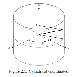
In the study of plane curves, it is common to use the frame ${\vec{T}, \vec{U}}$ to study the local properties of a plane curve $\vec{x}(t)$. (See [5, Chapter 1].) The vector $\vec{T}(t)$ is the unit tangent vector $\vec{T}(t)=\vec{x}^{\prime}(t) /\left|\vec{x}^{\prime}(t)\right|$, and the unit normal vector $\vec{U}(t)$, is the result of rotating $\vec{T}(t)$ by $\pi / 2$ in the counterclockwise direction. This is a moving frame that is defined in terms of a given regular curve $\vec{x}(t)$ and, at $t=t_{0}$, is viewed as based at the point $\vec{x}\left(t_{0}\right)$. To compare with applications in physics, it is important to note that the ${\vec{T}, \vec{U}}$ frame is not the same as the polar coordinate frame $\left{\vec{e}{r}, \vec{e}{\theta}\right}$. From Equation (2.4) (and ignoring the $z$-component), we know that
$$
\vec{e}{T}=(\cos \theta, \sin \theta) \quad \text { and } \quad \vec{e}{\theta}=(-\sin \theta, \cos \theta) .
$$
Assuming that $x, y, r$, and $\theta$ are functions of $t$ and since $x=r \cos \theta$ and $y=r \sin \theta$, we have
$$
\vec{x}^{\prime}(t)=\left(x^{\prime}(t), y^{\prime}(t)\right)=\left(r^{\prime} \cos \theta-r \theta^{\prime} \sin \theta, r^{\prime} \sin \theta+r \theta^{\prime} \cos \theta\right)=r^{\prime} \vec{e}{r}+r \theta^{\prime} \vec{e}{\theta} .
$$
We then calculate the speed function to be
$$
s^{\prime}(t)=\left|\vec{x}^{\prime}(t)\right|=\sqrt{\left(r^{\prime}\right)^{2}+r^{2}\left(\theta^{\prime}\right)^{2}}
$$
and find the unit tangent and unit normal vectors to be
$$
\begin{aligned}
&\vec{T}=\frac{1}{\sqrt{\left(r^{\prime}\right)^{2}+r^{2}\left(\theta^{r}\right)^{2}}}\left(r^{\prime} \vec{e}{r}+r \theta^{\prime} \vec{e}{\theta}\right), \
&\vec{U}=\frac{1}{\sqrt{\left(r^{\prime}\right)^{2}+r^{2}\left(\theta^{r}\right)^{2}}}\left(-r \theta^{\prime} \vec{e}{r}+r^{\prime} \vec{e}{\theta}\right) .
\end{aligned}
$$

数学代写|微分几何代写Differential Geometry代考|MATH 464

微分几何代考

数学代写|微分几何代写Differential Geometry代考| Frames Associated to Coordinate Systems

入门力学中的许多问题涉及在各种力的影响和/或受到某些约束的情况下找到粒子的轨迹。第一种方法使用坐标
函数,并将轨迹描述为
$$
\vec{r}(t)=(x(t), y(t), z(t))=x(t) \vec{\imath}+y(t) \vec{\jmath}+z(t) \vec{k} .
$$
然后,牛顿的运动方程导致三个坐标函数中的微分方程 $x(t), y(t)$ 和 $z(t)$. 速度函数是导数,即
$$
\vec{r}^{\prime}(t)=\frac{d}{d t}(x(t) \vec{\imath})+\frac{d}{d t}(y(t) \vec{\jmath})+\frac{d}{d t}(z(t) \vec{k}) \quad=x^{\prime}(t) \vec{\imath}+x(t) \frac{d}{d t}(\vec{\imath})+y^{\prime}(t) \vec{\jmath}+y(t) \frac{d}{d t}(\vec{\jmath})+z^{\prime}(t)
$$
因为 $\frac{d}{d t} \vec{\imath}=0, \frac{d}{d t} \vec{\jmath}=0$ 和 $\frac{d}{d t} \vec{k}=0$.最后一句话表明框架 $(\vec{\imath}, \vec{\jmath}, \vec{k})$ 与笛卡尔坐标系相关联的是一个常量坐标 系。
在讨论可变帧时,我们介绍了一种描述可变帧变化率的好方法。假设 $\vec{a}=a 1 \vec{u} 1+a 2 \vec{u} 2+a 3 \vec{u}{3}$ 和 $\vec{b}=b{1} \vec{u} 1+b 2 \vec{u} 2+b 3 \vec{u} 3$. 假设所有向量都是列向量,我们可以将这些组件 定义编写 $\vec{a}$ 和 $\vec{b}$ 在矩阵表达式中
使用这种符号,我们可以表达关系 $\frac{d}{d t} \vec{\imath}=0, \frac{d}{d t} \vec{j}=0$ 和 $\frac{d}{d t} \vec{k}=0$ 由

数学代写|微分几何代写Differential Geometry代考| Frames Associated to Trajectories

在轨迹研究中,无论是在物理学还是几何学中,使用与笛卡尔坐标系不同的标架通常都很方便。改变框架类型 有时会使困难的积分易于处理,或者使某些困难的微分方程易于管理。在狭义相对论的特定背景下,人们谈论 一个瞬时共动的参考系,缩写为MCRF。[50]
在平面曲线的研究中,通常使用框架 $\vec{T}, \vec{U}$ 以研究平面曲线的局部属性 $\vec{x}(t)$. (见[5,第1章]。向量 $\vec{T}(t)$ 是单位 切向量 $\vec{T}(t)=\vec{x}^{\prime}(t) /\left|\vec{x}^{\prime}(t)\right|$ 和单位法向量 $\vec{U}(t)$ ,是旋转的结果 $\vec{T}(t)$ 由 $\pi / 2$ 在逆时针方向上。这是一个移动 框架,根据给定的正则曲线定义 $\vec{x}(t)$ 和,在 $t=t_{0}$ ,被视为基于该点 $\vec{x}\left(t_{0}\right)$. 为了与物理学中的应用进行比较, 重要的是要注意 $\vec{T}, \vec{U}$ 框架与极坐标框架不同 Veft{\vec ${\mathrm{e}} r}$ ,Ivec{e}(theta}\right } } \text { . 从等式 (2.4) (并忽略 } z \text { -组 } 件),我们知道
$$
\vec{e} T=(\cos \theta, \sin \theta) \quad \text { and } \quad \vec{e} \theta=(-\sin \theta, \cos \theta) .
$$
假设 $x, y, r$ 和 $\theta$ 是 的函数 $t$ 和自 $x=r \cos \theta$ 和 $y=r \sin \theta$ 我们有
$$
\vec{x}^{\prime}(t)=\left(x^{\prime}(t), y^{\prime}(t)\right)=\left(r^{\prime} \cos \theta-r \theta^{\prime} \sin \theta, r^{\prime} \sin \theta+r \theta^{\prime} \cos \theta\right)=r^{\prime} \vec{e} r+r \theta^{\prime} \vec{e} \theta
$$
然后,我们将速度函数计算为
$$
s^{\prime}(t)=\left|\vec{x}^{\prime}(t)\right|=\sqrt{\left(r^{\prime}\right)^{2}+r^{2}\left(\theta^{\prime}\right)^{2}}
$$
并找到单位正切和单位法向量
$$
\vec{T}=\frac{1}{\sqrt{\left(r^{\prime}\right)^{2}+r^{2}\left(\theta^{r}\right)^{2}}}\left(r^{\prime} \vec{e} r+r \theta^{\prime} \vec{e} \theta\right), \quad \vec{U}=\frac{1}{\sqrt{\left(r^{\prime}\right)^{2}+r^{2}\left(\theta^{r}\right)^{2}}}\left(-r \theta^{\prime} \vec{e} r+r^{\prime} \vec{e} \theta\right) .
$$

数学代写|微分几何代写Differential Geometry代考 请认准statistics-lab™

统计代写请认准statistics-lab™. statistics-lab™为您的留学生涯保驾护航。

金融工程代写

金融工程是使用数学技术来解决金融问题。金融工程使用计算机科学、统计学、经济学和应用数学领域的工具和知识来解决当前的金融问题,以及设计新的和创新的金融产品。

非参数统计代写

非参数统计指的是一种统计方法,其中不假设数据来自于由少数参数决定的规定模型;这种模型的例子包括正态分布模型和线性回归模型。

广义线性模型代考

广义线性模型(GLM)归属统计学领域,是一种应用灵活的线性回归模型。该模型允许因变量的偏差分布有除了正态分布之外的其它分布。

术语 广义线性模型(GLM)通常是指给定连续和/或分类预测因素的连续响应变量的常规线性回归模型。它包括多元线性回归,以及方差分析和方差分析(仅含固定效应)。

有限元方法代写

有限元方法(FEM)是一种流行的方法,用于数值解决工程和数学建模中出现的微分方程。典型的问题领域包括结构分析、传热、流体流动、质量运输和电磁势等传统领域。

有限元是一种通用的数值方法,用于解决两个或三个空间变量的偏微分方程(即一些边界值问题)。为了解决一个问题,有限元将一个大系统细分为更小、更简单的部分,称为有限元。这是通过在空间维度上的特定空间离散化来实现的,它是通过构建对象的网格来实现的:用于求解的数值域,它有有限数量的点。边界值问题的有限元方法表述最终导致一个代数方程组。该方法在域上对未知函数进行逼近。[1] 然后将模拟这些有限元的简单方程组合成一个更大的方程系统,以模拟整个问题。然后,有限元通过变化微积分使相关的误差函数最小化来逼近一个解决方案。

tatistics-lab作为专业的留学生服务机构,多年来已为美国、英国、加拿大、澳洲等留学热门地的学生提供专业的学术服务,包括但不限于Essay代写,Assignment代写,Dissertation代写,Report代写,小组作业代写,Proposal代写,Paper代写,Presentation代写,计算机作业代写,论文修改和润色,网课代做,exam代考等等。写作范围涵盖高中,本科,研究生等海外留学全阶段,辐射金融,经济学,会计学,审计学,管理学等全球99%专业科目。写作团队既有专业英语母语作者,也有海外名校硕博留学生,每位写作老师都拥有过硬的语言能力,专业的学科背景和学术写作经验。我们承诺100%原创,100%专业,100%准时,100%满意。

随机分析代写


随机微积分是数学的一个分支,对随机过程进行操作。它允许为随机过程的积分定义一个关于随机过程的一致的积分理论。这个领域是由日本数学家伊藤清在第二次世界大战期间创建并开始的。

时间序列分析代写

随机过程,是依赖于参数的一组随机变量的全体,参数通常是时间。 随机变量是随机现象的数量表现,其时间序列是一组按照时间发生先后顺序进行排列的数据点序列。通常一组时间序列的时间间隔为一恒定值(如1秒,5分钟,12小时,7天,1年),因此时间序列可以作为离散时间数据进行分析处理。研究时间序列数据的意义在于现实中,往往需要研究某个事物其随时间发展变化的规律。这就需要通过研究该事物过去发展的历史记录,以得到其自身发展的规律。

回归分析代写

多元回归分析渐进(Multiple Regression Analysis Asymptotics)属于计量经济学领域,主要是一种数学上的统计分析方法,可以分析复杂情况下各影响因素的数学关系,在自然科学、社会和经济学等多个领域内应用广泛。

MATLAB代写

MATLAB 是一种用于技术计算的高性能语言。它将计算、可视化和编程集成在一个易于使用的环境中,其中问题和解决方案以熟悉的数学符号表示。典型用途包括:数学和计算算法开发建模、仿真和原型制作数据分析、探索和可视化科学和工程图形应用程序开发,包括图形用户界面构建MATLAB 是一个交互式系统,其基本数据元素是一个不需要维度的数组。这使您可以解决许多技术计算问题,尤其是那些具有矩阵和向量公式的问题,而只需用 C 或 Fortran 等标量非交互式语言编写程序所需的时间的一小部分。MATLAB 名称代表矩阵实验室。MATLAB 最初的编写目的是提供对由 LINPACK 和 EISPACK 项目开发的矩阵软件的轻松访问,这两个项目共同代表了矩阵计算软件的最新技术。MATLAB 经过多年的发展,得到了许多用户的投入。在大学环境中,它是数学、工程和科学入门和高级课程的标准教学工具。在工业领域,MATLAB 是高效研究、开发和分析的首选工具。MATLAB 具有一系列称为工具箱的特定于应用程序的解决方案。对于大多数 MATLAB 用户来说非常重要,工具箱允许您学习应用专业技术。工具箱是 MATLAB 函数(M 文件)的综合集合,可扩展 MATLAB 环境以解决特定类别的问题。可用工具箱的领域包括信号处理、控制系统、神经网络、模糊逻辑、小波、仿真等。

R语言代写问卷设计与分析代写
PYTHON代写回归分析与线性模型代写
MATLAB代写方差分析与试验设计代写
STATA代写机器学习/统计学习代写
SPSS代写计量经济学代写
EVIEWS代写时间序列分析代写
EXCEL代写深度学习代写
SQL代写各种数据建模与可视化代写

数学代写|微分几何代写Differential Geometry代考|MATH4030

如果你也在 怎样代写微分几何Differential Geometry这个学科遇到相关的难题,请随时右上角联系我们的24/7代写客服。

微分几何学是一门研究光滑形状和光滑空间的几何学的数学学科,也被称为光滑流形。它使用微分计算、积分计算、线性代数和多线代数的技术。

statistics-lab™ 为您的留学生涯保驾护航 在代写微分几何Differential Geometry方面已经树立了自己的口碑, 保证靠谱, 高质且原创的统计Statistics代写服务。我们的专家在代写微分几何Differential Geometry代写方面经验极为丰富,各种代写微分几何Differential Geometry相关的作业也就用不着说。

我们提供的微分几何Differential Geometry及其相关学科的代写,服务范围广, 其中包括但不限于:

  • Statistical Inference 统计推断
  • Statistical Computing 统计计算
  • Advanced Probability Theory 高等概率论
  • Advanced Mathematical Statistics 高等数理统计学
  • (Generalized) Linear Models 广义线性模型
  • Statistical Machine Learning 统计机器学习
  • Longitudinal Data Analysis 纵向数据分析
  • Foundations of Data Science 数据科学基础
数学代写|微分几何代写Differential Geometry代考|MATH4030

数学代写|微分几何代写Differential Geometry代考|Differentiation Rules; Functions of Class C

In a single-variable calculus course, one learns a number of differentiation rules. With functions $F$ from $\mathbb{R}^{n}$ to $\mathbb{R}^{m}$, one must use some caution since the matrix $[d F]$ of the differential $d F$ is not a vector function but a matrix of functions. (Again, we remind the reader that our notation for evaluating the matrix of functions $[d F]$ at a point $\vec{a}$ is $\left[d F_{\vec{a}}\right]$.)

Theorem 1.3.1. Let $U$ be an open set in $\mathbb{R}^{n}$. Let $F$ and $G$ be functions from $U$ to $\mathbb{R}^{m}$, and let $w: U \rightarrow \mathbb{R}$ be a scalar function. If $F, G$, and $w$ are differentiable at $\vec{a}$, then $F+G$ and $w F$ are differentiable at $\vec{a}$ and

  1. $d(F+G){\vec{a}}=d F{\vec{a}}+d G_{\vec{a}}$;
  2. $\left[d(w F){\vec{a}}\right]=w(\vec{a})\left[d F{\vec{a}}\right]+[F(\vec{a})]\left[d w_{\vec{a}}\right]$.
    Proof. The proof for both parts follows from Proposition 1.2.17. Explicitly for the second part, the $i j$-entry of $\left[d(w F){\vec{a}}\right]$ is $$ \frac{\partial\left(w F{i}\right)}{\partial x_{j}}=w(\vec{a}) \frac{\partial F_{i}}{\partial x_{j}}(\vec{a})+\frac{\partial w}{\partial x_{j}}(\vec{a}) F_{i}(\vec{a}) .
    $$
    The first term on the right side is the $i j$-entry of $w(\vec{a})\left[d F_{\vec{a}}\right]$ while the second term is the $i j$-entry of $[F(\vec{a})]\left[d w_{\vec{a}}\right]$, which is the product of a columns by a row vector. The result follows.

Note that in Theorem 1.3.1(2), $[F(\vec{a})]$ is a column vector of dimension $m$, while $\left[d w_{\vec{a}}\right]$ is a row vector of dimension $n$. Hence $[F(\vec{a})]\left[d w_{\vec{a}}\right]$ is an $m \times n$ matrix of rank $1 .$

数学代写|微分几何代写Differential Geometry代考|Inverse and Implicit Function Theorems

In single- and multivariable calculus of a function $F: \mathbb{R}^{n} \rightarrow \mathbb{R}$, one defines a critical point as a point $\vec{a}=\left(a_{1}, \ldots, a_{n}\right)$ such that the gradient of $F$ at $\vec{a}$ is $\overrightarrow{0}$, i.e.,
$$
\nabla F(\vec{a})=\left(\frac{\partial F}{\partial x_{1}}(\vec{a}), \ldots, \frac{\partial F}{\partial x_{n}}(\vec{a})\right)=\overrightarrow{0}
$$
At such a point, $F$ is said to have a flat tangent line or tangent plane, and, according to standard theorems in calculus, $F(\vec{a})$ is either a local minimum, local maximum, or a “saddle point.” This notion is a special case of the following general definition.
Definition 1.4.1. Let $U$ be an open subset of $\mathbb{R}^{n}$ and $F: U \rightarrow \mathbb{R}^{m}$ a differentiable function. We call $q \in U$ a critical point of $F$ if $F$ is not differentiable at $q$ or if $d F_{q}: \mathbb{R}^{n} \rightarrow \mathbb{R}^{m}$ is not of maximum rank, i.e., if $\operatorname{rank}\left(d F_{q}\right)<\min (m, n)$. If $q$ is a critical point of $F$, we call $F(q)$ a critical value. If $p \in \mathbb{R}^{m}$ is not a critical value of $F$ (even if $p$ is not in the image of $F$ ), then we call $p$ a regular value of $F$.

We point out that this definition simultaneously generalizes the notion of a critical point for functions $F: U \rightarrow \mathbb{R}$, with $U$ an open subset of $\mathbb{R}^{n}$, and the definition for a critical point of a parametric curve in $\mathbb{R}^{n}$ (Definition $3.2 .1$ in $[5]$ ). If $m=n$, the notion of a critical point has a few alternate equivalent criteria.

数学代写|微分几何代写Differential Geometry代考|MATH4030

微分几何代考

数学代写|微分几何代写Differential Geometry代考| Differentiation Rules; Functions of Class C

在单变量微积分课程中,人们学习了许多微分规则。带函数 $F$ 从 $\mathbb{R}^{n}$ 自 $\mathbb{R}^{m}$ ,必须谨慎使用,因为矩阵 $[d F]$ 的差 分 $d F$ 不是向量函数,而是函数矩阵。(再次,我们提醒读者,我们用于计算函数矩阵的符号 $[d F]$ 在某一点 $\vec{a}$ 是 $\left.\left[d F_{\vec{a}}\right] .\right)$
定理 1.3.1. 让 $U$ 成为开放的集合 $\mathbb{R}^{n}$. 让 $F$ 和 $G$ 函数来自 $U$ 自 $\mathbb{R}^{m}$ ,并让 $w: U \rightarrow \mathbb{R}$ 是一个标量函数。如果 $F, G$ 和 $w$ 在 $\vec{a}$ 然后 $F+G$ 和 $w F$ 在 $\vec{a}$ 和

  1. $d(F+G) \vec{a}=d F \vec{a}+d G_{\vec{a}}$
  2. $[d(w F) \vec{a}]=w(\vec{a})[d F \vec{a}]+[F(\vec{a})]\left[d w_{\vec{a}}\right]$.
    证明。这两个部分的证明都来自命题1.2.17。明确地对于第二部分, $i j$-进入 $[d(w F) \vec{a}]$ 是
    $$
    \frac{\partial(w F i)}{\partial x_{j}}=w(\vec{a}) \frac{\partial F_{i}}{\partial x_{j}}(\vec{a})+\frac{\partial w}{\partial x_{j}}(\vec{a}) F_{i}(\vec{a}) .
    $$
    右侧的第一个术语是 $i j$-进入 $w(\vec{a})\left[d F_{\vec{a}}\right]$ 而第二个术语是 $i j$-进入 $[F(\vec{a})]\left[d w_{\vec{a}}\right]$ ,它是列乘以行向量的乘 积。结果如下。
    请注意,在定理 $1.3 .1$ (2) 中, $[F(\vec{a})]$ 是维度的列向量 $m$ 而 $\left[d w_{\vec{a}}\right]$ 是维度的行向量 $n$. 因此 $[F(\vec{a})]\left[d w_{\vec{a}}\right]$ 是一个 $m \times n$ 等级矩阵 1 .

数学代写|微分几何代写Differential Geometry代考| Inverse and Implicit Function Theorems

在函数的单变量和多变量微积分中 $F: \mathbb{R}^{n} \rightarrow \mathbb{R}$ ,将临界点定义为点 $\vec{a}=\left(a_{1}, \ldots, a_{n}\right)$ 使得梯度 $F$ 在 $\vec{a}$ 是 $\overrightarrow{0}$ , 即
$$
\nabla F(\vec{a})=\left(\frac{\partial F}{\partial x_{1}}(\vec{a}), \ldots, \frac{\partial F}{\partial x_{n}}(\vec{a})\right)=\overrightarrow{0}
$$
在这一点上,F据说具有平坦的切线或切平面,并且根据微积分中的标准定理, $F(\vec{a})$ 是局部最小值、局部最大 值或”鞍点”。这个概念是以下一般定义的一个特例。
定义 1.4.1.让 $U$ 是的开放子集 $\mathbb{R}^{n}$ 和 $F: U \rightarrow \mathbb{R}^{m}$ 可微函数。我们调用 $q \in U$ 一个关键点 $F$ 如果 $F$ 在 $q$ 或者如果 $d F_{q}: \mathbb{R}^{n} \rightarrow \mathbb{R}^{m}$ 不是最高等级,即 $\operatorname{rank}\left(d F_{q}\right)<\min (m, n)$. 如果 $q$ 是 $F$ ,我们称之为 $F(q)$ 一个临界值。 如果 $p \in \mathbb{R}^{m}$ 不是的临界值 $F$ (即使 $p$ 不在图像中 $F$ ),然后我们调用 $p$ 常规值 $F$.
我们指出,这个定义同时推广了函数临界点的概念。 $F: U \rightarrow \mathbb{R}$ 跟 $U$ 的开放子集 $\mathbb{R}^{n}$ ,以及参数化曲线的临界 点的定义 $\mathbb{R}^{n}$ (定义 $3.2 .1$ 在 $\left.[5]\right)$ ).如果 $m=n$ ,临界点的概念有一些替代的等价标准。

数学代写|微分几何代写Differential Geometry代考 请认准statistics-lab™

统计代写请认准statistics-lab™. statistics-lab™为您的留学生涯保驾护航。

金融工程代写

金融工程是使用数学技术来解决金融问题。金融工程使用计算机科学、统计学、经济学和应用数学领域的工具和知识来解决当前的金融问题,以及设计新的和创新的金融产品。

非参数统计代写

非参数统计指的是一种统计方法,其中不假设数据来自于由少数参数决定的规定模型;这种模型的例子包括正态分布模型和线性回归模型。

广义线性模型代考

广义线性模型(GLM)归属统计学领域,是一种应用灵活的线性回归模型。该模型允许因变量的偏差分布有除了正态分布之外的其它分布。

术语 广义线性模型(GLM)通常是指给定连续和/或分类预测因素的连续响应变量的常规线性回归模型。它包括多元线性回归,以及方差分析和方差分析(仅含固定效应)。

有限元方法代写

有限元方法(FEM)是一种流行的方法,用于数值解决工程和数学建模中出现的微分方程。典型的问题领域包括结构分析、传热、流体流动、质量运输和电磁势等传统领域。

有限元是一种通用的数值方法,用于解决两个或三个空间变量的偏微分方程(即一些边界值问题)。为了解决一个问题,有限元将一个大系统细分为更小、更简单的部分,称为有限元。这是通过在空间维度上的特定空间离散化来实现的,它是通过构建对象的网格来实现的:用于求解的数值域,它有有限数量的点。边界值问题的有限元方法表述最终导致一个代数方程组。该方法在域上对未知函数进行逼近。[1] 然后将模拟这些有限元的简单方程组合成一个更大的方程系统,以模拟整个问题。然后,有限元通过变化微积分使相关的误差函数最小化来逼近一个解决方案。

tatistics-lab作为专业的留学生服务机构,多年来已为美国、英国、加拿大、澳洲等留学热门地的学生提供专业的学术服务,包括但不限于Essay代写,Assignment代写,Dissertation代写,Report代写,小组作业代写,Proposal代写,Paper代写,Presentation代写,计算机作业代写,论文修改和润色,网课代做,exam代考等等。写作范围涵盖高中,本科,研究生等海外留学全阶段,辐射金融,经济学,会计学,审计学,管理学等全球99%专业科目。写作团队既有专业英语母语作者,也有海外名校硕博留学生,每位写作老师都拥有过硬的语言能力,专业的学科背景和学术写作经验。我们承诺100%原创,100%专业,100%准时,100%满意。

随机分析代写


随机微积分是数学的一个分支,对随机过程进行操作。它允许为随机过程的积分定义一个关于随机过程的一致的积分理论。这个领域是由日本数学家伊藤清在第二次世界大战期间创建并开始的。

时间序列分析代写

随机过程,是依赖于参数的一组随机变量的全体,参数通常是时间。 随机变量是随机现象的数量表现,其时间序列是一组按照时间发生先后顺序进行排列的数据点序列。通常一组时间序列的时间间隔为一恒定值(如1秒,5分钟,12小时,7天,1年),因此时间序列可以作为离散时间数据进行分析处理。研究时间序列数据的意义在于现实中,往往需要研究某个事物其随时间发展变化的规律。这就需要通过研究该事物过去发展的历史记录,以得到其自身发展的规律。

回归分析代写

多元回归分析渐进(Multiple Regression Analysis Asymptotics)属于计量经济学领域,主要是一种数学上的统计分析方法,可以分析复杂情况下各影响因素的数学关系,在自然科学、社会和经济学等多个领域内应用广泛。

MATLAB代写

MATLAB 是一种用于技术计算的高性能语言。它将计算、可视化和编程集成在一个易于使用的环境中,其中问题和解决方案以熟悉的数学符号表示。典型用途包括:数学和计算算法开发建模、仿真和原型制作数据分析、探索和可视化科学和工程图形应用程序开发,包括图形用户界面构建MATLAB 是一个交互式系统,其基本数据元素是一个不需要维度的数组。这使您可以解决许多技术计算问题,尤其是那些具有矩阵和向量公式的问题,而只需用 C 或 Fortran 等标量非交互式语言编写程序所需的时间的一小部分。MATLAB 名称代表矩阵实验室。MATLAB 最初的编写目的是提供对由 LINPACK 和 EISPACK 项目开发的矩阵软件的轻松访问,这两个项目共同代表了矩阵计算软件的最新技术。MATLAB 经过多年的发展,得到了许多用户的投入。在大学环境中,它是数学、工程和科学入门和高级课程的标准教学工具。在工业领域,MATLAB 是高效研究、开发和分析的首选工具。MATLAB 具有一系列称为工具箱的特定于应用程序的解决方案。对于大多数 MATLAB 用户来说非常重要,工具箱允许您学习应用专业技术。工具箱是 MATLAB 函数(M 文件)的综合集合,可扩展 MATLAB 环境以解决特定类别的问题。可用工具箱的领域包括信号处理、控制系统、神经网络、模糊逻辑、小波、仿真等。

R语言代写问卷设计与分析代写
PYTHON代写回归分析与线性模型代写
MATLAB代写方差分析与试验设计代写
STATA代写机器学习/统计学习代写
SPSS代写计量经济学代写
EVIEWS代写时间序列分析代写
EXCEL代写深度学习代写
SQL代写各种数据建模与可视化代写

数学代写|微分几何代写Differential Geometry代考|MATH3405

如果你也在 怎样代写微分几何Differential Geometry这个学科遇到相关的难题,请随时右上角联系我们的24/7代写客服。

微分几何学是一门研究光滑形状和光滑空间的几何学的数学学科,也被称为光滑流形。它使用微分计算、积分计算、线性代数和多线代数的技术。

statistics-lab™ 为您的留学生涯保驾护航 在代写微分几何Differential Geometry方面已经树立了自己的口碑, 保证靠谱, 高质且原创的统计Statistics代写服务。我们的专家在代写微分几何Differential Geometry代写方面经验极为丰富,各种代写微分几何Differential Geometry相关的作业也就用不着说。

我们提供的微分几何Differential Geometry及其相关学科的代写,服务范围广, 其中包括但不限于:

  • Statistical Inference 统计推断
  • Statistical Computing 统计计算
  • Advanced Probability Theory 高等概率论
  • Advanced Mathematical Statistics 高等数理统计学
  • (Generalized) Linear Models 广义线性模型
  • Statistical Machine Learning 统计机器学习
  • Longitudinal Data Analysis 纵向数据分析
  • Foundations of Data Science 数据科学基础
数学代写|微分几何代写Differential Geometry代考|MATH3405

数学代写|微分几何代写Differential Geometry代考|Analysis of Multivariable Functions

Let $U$ be a subset of $\mathbb{R}^{n}$ and let $f: U \rightarrow \mathbb{R}^{m}$ be a function from $U$ to $\mathbb{R}^{m}$. Writing the input variable as
$$
\vec{x}=\left(x_{1}, x_{2}, \ldots, x_{n}\right),
$$
we denote the output assigned to $\vec{x}$ by $f(\vec{x})$ or $f\left(x_{1}, \ldots, x_{n}\right)$. Since the codomain of $f$ is $\mathbb{R}^{m}$, the images of $f$ are $m$-tuples so we can write
$$
\begin{aligned}
f(\vec{x}) &=\left(f_{1}(\vec{x}), f_{2}(\vec{x}), \ldots, f_{m}(\vec{x})\right) \
&=\left(f_{1}\left(x_{1}, x_{2}, \ldots, x_{n}\right), f_{2}\left(x_{1}, x_{2}, \ldots, x_{n}\right), \ldots, f_{m}\left(x_{1}, x_{2}, \ldots, x_{n}\right)\right) .
\end{aligned}
$$
The functions $f_{i}: U \rightarrow \mathbb{R}$, for $i=1,2, \ldots, m$, are called the component functions of $f$.

We sometimes use the notation $\vec{f}(\vec{x})$ to emphasize the fact that the codomain $\mathbb{R}^{m}$ is a vector space and that any operation on $m$-dimensional vectors is permitted on functions $\vec{f}: \mathbb{R}^{n} \rightarrow \mathbb{R}^{m}$. Therefore, some authors call such functions vector functions of a vector variable.

In any Euclidean space $\mathbb{R}^{n}$, the standard basis is the set of vectors written as $\left{\vec{e}{1}, \vec{e}{2}, \ldots, \vec{e}{n}\right}$, where $$ \vec{e}{i}=\left(\begin{array}{c}
0 \
\vdots \
1 \
\vdots \
0
\end{array}\right)
$$
with the only nonzero entry 1 occurring in the $i$ th coordinate. If no basis is explicitly specified for $\mathbb{R}^{n}$, then it is assumed that one uses the standard basis.

At this point, a remark is in order concerning the differences in notations between calculus and linear algebra. In calculus, one usually denotes an element of $\mathbb{R}^{n}$ as an $n$-tuple and writes this element on one line as $\left(x_{1}, x_{2}, \ldots, x_{n}\right)$. On the other hand, in order to reconcile vector notation with the usual manner we multiply a matrix by a vector, in linear algebra we denote an element of $\mathbb{R}^{n}$ as a column vector
$$
\vec{x}=\left(\begin{array}{c}
x_{1} \
x_{2} \
\vdots \
x_{n}
\end{array}\right)
$$

数学代写|微分几何代写Differential Geometry代考|Continuity, Limits, and Differentiability

Intuitively, a function is called continuous if it preserves “nearness.” A rigorous mathematical definition for continuity for functions from $\mathbb{R}^{n}$ to $\mathbb{R}^{m}$ is hardly any different for functions from $\mathbb{R} \rightarrow \mathbb{R}$.

In calculus of a real variable, one does not study functions defined over a discrete set of real values because the notions behind continuity and differentiability do not make sense over such sets. Instead, one often assumes the function is defined over some interval. Similarly, for the analysis of functions $\mathbb{R}^{n}$ to $\mathbb{R}^{m}$, one does not study functions defined from any subset of $\mathbb{R}^{n}$ into $\mathbb{R}^{m}$. One typically considers functions defined over what is called an open set in $\mathbb{R}^{n}$, a notion we define now.
Definition 1.2.1. The open ball around $\vec{x}{0}$ of radius $r$ is the set $$ B{r}\left(\vec{x}{0}\right)=\left{\vec{x} \in \mathbb{R}^{n}:\left|\vec{x}-\vec{x}{0}\right|0$ such that $B_{r}(\vec{x}) \subset U$.

Intuitively speaking, the definition of an open set $U$ in $\mathbb{R}^{n}$ implies that at every point $p \in U$ it is possible to “move” in any direction by at least a little amount $\epsilon$ and still remain in $U$. This means that in some sense $U$ captures the full dimensionality of the ambient space $\mathbb{R}^{n}$. This is why, when studying the analysis of functions from $\mathbb{R}^{n}$ to $\mathbb{R}^{m}$, we narrow our attention to functions $F: U \rightarrow \mathbb{R}^{m}$, where $U$ is an open subset of $\mathbb{R}^{n}$.

The reader is encouraged to consult Subsection A.1.2 in Appendix A for more background on open and closed sets. The situation in which we need to consider an open set $U$ and a point $\vec{x}_{0}$ in $U$ is so common that another terminology exists for $U$ in this case.

Definition 1.2.2. Let $\vec{x}{0} \in \mathbb{R}^{n}$. Any open set $U$ in $\mathbb{R}^{n}$ such that $\vec{x}{0} \in U$ is called an open neighborhood, or more simply, a neighborhood, of $\vec{x}{0}$. We are now in a position to formally define continuity. Definition 1.2.3. Let $U$ be an open subset of $\mathbb{R}^{n}$, and let $F$ be a function from $U$ into $\mathbb{R}^{m}$. The function $F$ is called continuous at the point $\vec{x}{0} \in U$ if $F\left(\vec{x}{0}\right)$ exists and if, for all $\varepsilon>0$, there exists a $\delta>0$ such that for all $\vec{x} \in \mathbb{R}$, $$ \left|\vec{x}-\vec{x}{0}\right|<\delta \Longrightarrow\left|F(\vec{x})-F\left(\vec{x}_{0}\right)\right|<\epsilon .
$$
The function $F$ is called continuous on $U$ if it is continuous at every point of $U$.

数学代写|微分几何代写Differential Geometry代考|MATH3405

微分几何代考

数学代写|微分几何代写Differential Geometry代考| Analysis of Multivariable Functions

让 $U$ 是 的子集 $\mathbb{R}^{n}$ 并让 $f: U \rightarrow \mathbb{R}^{m}$ 是来自 $U$ 自 $\mathbb{R}^{m}$. 将输入变量编写为
$$
\vec{x}=\left(x_{1}, x_{2}, \ldots, x_{n}\right),
$$
我们表示分配给 $\vec{x}$ 由 $f(\vec{x})$ 或 $f\left(x_{1}, \ldots, x_{n}\right)$. 自共域以来 $f$ 是 $\mathbb{R}^{m}$ ,图像 $f$ 是 $m$-元组,所以我们可以写
$$
f(\vec{x})=\left(f_{1}(\vec{x}), f_{2}(\vec{x}), \ldots, f_{m}(\vec{x})\right) \quad=\left(f_{1}\left(x_{1}, x_{2}, \ldots, x_{n}\right), f_{2}\left(x_{1}, x_{2}, \ldots, x_{n}\right), \ldots, f_{m}\left(x_{1}, x_{2},\right.\right.
$$
功能 $f_{i}: U \rightarrow \mathbb{R}$ 为 $i=1,2, \ldots, m$ ,称为 的组件函数 $f$.
我们有时使用符号 $\vec{f}(\vec{x})$ 强调共域的事实 $\mathbb{R}^{m}$ 是一个向量空间,并且对 $m$-函数上允许使用维向量 $\vec{f}: \mathbb{R}^{n} \rightarrow \mathbb{R}^{m}$. 因此,一些作者将此类函数称为向量变量的向量函数。
在任何欧几里得空间中 $\mathbb{R}^{n}$ ,标准基础是向量的集合,写为 Veft {lvec{e}{1},Ivec{e}2},Vdots,Ivec{e}n}\right } } 哪里
$$
\vec{e} i=(0 \vdots 1 \vdots 0)
$$
唯一的非零条目 1 出现在 $i$ th 坐标。如果没有明确指定基础 $\mathbb{R}^{n}$ ,则假定使用标准基。
在这一点上,关于微积分和线性代数之间符号的差异,有必要进行一些评论。在微积分中,一个通常表示 $\mathbb{R}^{n}$ 作 为 $n$-元组,并将此元素写在一行上 $\left(x_{1}, x_{2}, \ldots, x_{n}\right)$. 另一方面,为了调和向量符号与通常的方式,我们将矩阵 乘以向量,在线性代数中,我们表示 $\mathbb{R}^{n}$ 作为列向量
$$
\vec{x}=\left(x_{1} x_{2} \vdots x_{n}\right)
$$

数学代写|微分几何代写Differential Geometry代考| Continuity, Limits, and Differentiability

直观地说,如果函数保持”接近性”,则称为连续函数。函数连续性的严格数学定义 $\mathbb{R}^{n}$ 自 $\mathbb{R}^{m}$ 对于函数几乎没有 任何区别 $\mathbb{R} \rightarrow \mathbb{R}$.
在实变量的演算中,人们不研究在一组离散的实数值上定义的函数,因为连续性和可微性背后的概念在这些集 合上没有意义。相反,人们通常假设函数是在某个时间间隔内定义的。同样,用于函数分析 $\mathbb{R}^{n}$ 自 $\mathbb{R}^{m}$ ,则不研 究从 的任何子集定义的函数 $\mathbb{R}^{n}$ 到 $\mathbb{R}^{m}$. 人们通常认为在所谓的开集上定义的函数 $\mathbb{R}^{n}$ ,我们现在定义的一个概 念。
定义 1.2.1.周围的开口球 $\vec{x} 0$ 半径 $r$ is the set $\$ \$ B{r} \backslash$ eft $($ Vec ${x}{0} \backslash r i g h t)=V$ left ${$ lvec ${x} \backslash$ in Imathbb ${R} \wedge{\mathrm{n}}$ : Veft|Ivec ${x}-\mid \operatorname{vec}{x}{0} \backslash$ right $\mid 0$ suchthatB_{r} (Ivec ${\mathrm{x}})$ Isubset U\$.
直观地说,开集的定义 $U$ 在 $\mathbb{R}^{n}$ 意味着在每一点上 $p \in U$ 可以向任何方向“移动”至少一点点 $\epsilon$ 并仍然留在 $U$. 这意 味着在某种意义上 $U$ 捕获环境空间的全部维度 $\mathbb{R}^{n}$. 伩就是为什么在研究函数分析时 $\mathbb{R}^{n}$ 自 $\mathbb{R}^{m}$ ,我们将注意力缩 小到函数 $F: U \rightarrow \mathbb{R}^{m}$ 哪里 $U$ 是 的开放子集 $\mathbb{R}^{n}$.
鼓励读者查阅附录A中的A.1.2小节,了解有关开放和封闭集合的更多背景知识。我们需要考虑一个开放集合的 情况 $U$ 和一个点 $\vec{x}{0}$ 在 $U$ 是如此普遍,以至于存在另一个术语 $U$ 在这种情况下。 定义 1.2.2.让 $\vec{x} 0 \in \mathbb{R}^{n}$.任何打开的集合 $U$ 在 $\mathbb{R}^{n}$ 使得 $\vec{x} 0 \in U$ 被称为开放邻域,或更简单地说,称为邻域 $\vec{x} 0$.我 们现在能够正式界定连续性。定义 1.2.3.让 $U$ 是 的开放子集 $\mathbb{R}^{n}$ ,并让 $F$ 是来自 $U$ 到 $\mathbb{R}^{m}$. 功能 $F$ 在点处称为连续 $\vec{x} 0 \in U$ 如果 $F(\vec{x} 0)$ 存在和如果,对于所有 $\varepsilon>0$ ,则存在一个 $\delta>0$ 这样,对于所有 $\vec{x} \in \mathbb{R}$ , $$ |\vec{x}-\vec{x} 0|<\delta \Longrightarrow\left|F(\vec{x})-F\left(\vec{x}{0}\right)\right|<\epsilon .
$$
功能 $F$ 称为 连续于 $U$ 如果它在以下每个点上都是连续的 $U$.

数学代写|微分几何代写Differential Geometry代考 请认准statistics-lab™

统计代写请认准statistics-lab™. statistics-lab™为您的留学生涯保驾护航。

金融工程代写

金融工程是使用数学技术来解决金融问题。金融工程使用计算机科学、统计学、经济学和应用数学领域的工具和知识来解决当前的金融问题,以及设计新的和创新的金融产品。

非参数统计代写

非参数统计指的是一种统计方法,其中不假设数据来自于由少数参数决定的规定模型;这种模型的例子包括正态分布模型和线性回归模型。

广义线性模型代考

广义线性模型(GLM)归属统计学领域,是一种应用灵活的线性回归模型。该模型允许因变量的偏差分布有除了正态分布之外的其它分布。

术语 广义线性模型(GLM)通常是指给定连续和/或分类预测因素的连续响应变量的常规线性回归模型。它包括多元线性回归,以及方差分析和方差分析(仅含固定效应)。

有限元方法代写

有限元方法(FEM)是一种流行的方法,用于数值解决工程和数学建模中出现的微分方程。典型的问题领域包括结构分析、传热、流体流动、质量运输和电磁势等传统领域。

有限元是一种通用的数值方法,用于解决两个或三个空间变量的偏微分方程(即一些边界值问题)。为了解决一个问题,有限元将一个大系统细分为更小、更简单的部分,称为有限元。这是通过在空间维度上的特定空间离散化来实现的,它是通过构建对象的网格来实现的:用于求解的数值域,它有有限数量的点。边界值问题的有限元方法表述最终导致一个代数方程组。该方法在域上对未知函数进行逼近。[1] 然后将模拟这些有限元的简单方程组合成一个更大的方程系统,以模拟整个问题。然后,有限元通过变化微积分使相关的误差函数最小化来逼近一个解决方案。

tatistics-lab作为专业的留学生服务机构,多年来已为美国、英国、加拿大、澳洲等留学热门地的学生提供专业的学术服务,包括但不限于Essay代写,Assignment代写,Dissertation代写,Report代写,小组作业代写,Proposal代写,Paper代写,Presentation代写,计算机作业代写,论文修改和润色,网课代做,exam代考等等。写作范围涵盖高中,本科,研究生等海外留学全阶段,辐射金融,经济学,会计学,审计学,管理学等全球99%专业科目。写作团队既有专业英语母语作者,也有海外名校硕博留学生,每位写作老师都拥有过硬的语言能力,专业的学科背景和学术写作经验。我们承诺100%原创,100%专业,100%准时,100%满意。

随机分析代写


随机微积分是数学的一个分支,对随机过程进行操作。它允许为随机过程的积分定义一个关于随机过程的一致的积分理论。这个领域是由日本数学家伊藤清在第二次世界大战期间创建并开始的。

时间序列分析代写

随机过程,是依赖于参数的一组随机变量的全体,参数通常是时间。 随机变量是随机现象的数量表现,其时间序列是一组按照时间发生先后顺序进行排列的数据点序列。通常一组时间序列的时间间隔为一恒定值(如1秒,5分钟,12小时,7天,1年),因此时间序列可以作为离散时间数据进行分析处理。研究时间序列数据的意义在于现实中,往往需要研究某个事物其随时间发展变化的规律。这就需要通过研究该事物过去发展的历史记录,以得到其自身发展的规律。

回归分析代写

多元回归分析渐进(Multiple Regression Analysis Asymptotics)属于计量经济学领域,主要是一种数学上的统计分析方法,可以分析复杂情况下各影响因素的数学关系,在自然科学、社会和经济学等多个领域内应用广泛。

MATLAB代写

MATLAB 是一种用于技术计算的高性能语言。它将计算、可视化和编程集成在一个易于使用的环境中,其中问题和解决方案以熟悉的数学符号表示。典型用途包括:数学和计算算法开发建模、仿真和原型制作数据分析、探索和可视化科学和工程图形应用程序开发,包括图形用户界面构建MATLAB 是一个交互式系统,其基本数据元素是一个不需要维度的数组。这使您可以解决许多技术计算问题,尤其是那些具有矩阵和向量公式的问题,而只需用 C 或 Fortran 等标量非交互式语言编写程序所需的时间的一小部分。MATLAB 名称代表矩阵实验室。MATLAB 最初的编写目的是提供对由 LINPACK 和 EISPACK 项目开发的矩阵软件的轻松访问,这两个项目共同代表了矩阵计算软件的最新技术。MATLAB 经过多年的发展,得到了许多用户的投入。在大学环境中,它是数学、工程和科学入门和高级课程的标准教学工具。在工业领域,MATLAB 是高效研究、开发和分析的首选工具。MATLAB 具有一系列称为工具箱的特定于应用程序的解决方案。对于大多数 MATLAB 用户来说非常重要,工具箱允许您学习应用专业技术。工具箱是 MATLAB 函数(M 文件)的综合集合,可扩展 MATLAB 环境以解决特定类别的问题。可用工具箱的领域包括信号处理、控制系统、神经网络、模糊逻辑、小波、仿真等。

R语言代写问卷设计与分析代写
PYTHON代写回归分析与线性模型代写
MATLAB代写方差分析与试验设计代写
STATA代写机器学习/统计学习代写
SPSS代写计量经济学代写
EVIEWS代写时间序列分析代写
EXCEL代写深度学习代写
SQL代写各种数据建模与可视化代写