如果你也在 怎样代写概率与统计Probability and Statistics这个学科遇到相关的难题，请随时右上角联系我们的24/7代写客服。

概率涉及预测未来事件的可能性，而统计涉及对过去事件频率的分析。概率论主要是数学的一个理论分支，它研究数学定义的后果。

statistics-lab™ 为您的留学生涯保驾护航 在代写概率与统计Probability and Statistics方面已经树立了自己的口碑, 保证靠谱, 高质且原创的统计Statistics代写服务。我们的专家在代写概率与统计Probability and Statistics方面经验极为丰富，各种代写概率与统计Probability and Statistics相关的作业也就用不着说。

我们提供的概率与统计Probability and Statistics及其相关学科的代写，服务范围广, 其中包括但不限于:

• Statistical Inference 统计推断
• Statistical Computing 统计计算
• Advanced Probability Theory 高等楖率论
• Advanced Mathematical Statistics 高等数理统计学
• (Generalized) Linear Models 广义线性模型
• Statistical Machine Learning 统计机器学习
• Longitudinal Data Analysis 纵向数据分析
• Foundations of Data Science 数据科学基础

统计代写|概率与统计作业代写Probability and Statistics代考|Dispersion, Skewness, and Kurtosis

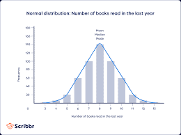
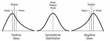
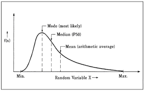
Knowing the “central tendency” or locations of data points might not be sufficient to really understand the data that you are looking at. Dispersion measures help us understand how far apart the data are away from the center or from each other, while skewness and kurtosis are measures that describe features of the shape of the frequency plot of the data.

1. Range and interquartile range: Range is the difference between the maximum and minimum. It quantifies the maximum distance between any two data points. The range is easy to calculate in $\mathrm{R}$ :
   $>\max$ (face_data\$rating) – $\min$ (face_data\$rating)
   [1] 99
   Clearly, the range is sensitive to outliers. Instead of using the minimum and maximum, we could use the difference between two quantiles to circumvent the problem of outliers. The interquartile range (IQR) calculates the difference between the third quartile and the first quartile. It quantifies a range for which $50 \%$ of the data falls within.

Thus $50 \%$ of the rating data lies within a range of 37 . The interquartile range is visualized in the boxplot, which we discuss later in this chapter.

2. Mean absolute deviation: We can also compute the average distance that data values are away from the mean:
   $$
   M A D=\frac{1}{n} \sum_{i=1}^n\left|x_i-\bar{x}\right|
   $$ where $|\cdot|$ denotes the absolute value. $R$ does not have a built-in function for this, but $M A D$ can easily be computed in $\mathrm{R}$ :
3. $>\operatorname{sum}(\operatorname{abs}(x-\operatorname{mean}(x))) /$ length $(x)$

3. Mean squared deviation, variance, and standard deviation: Much more common than the mean absolute difference is the mean squared deviation about the mean:
   $$
   M S D=\frac{1}{n} \sum_{i=1}^n\left(x_i-\bar{x}\right)^2
   $$
   It does the same as $M A D$, but now it uses squared distances with respect to the mean. The variance is almost identical to the mean squared deviation, since it is given by $s^2=\sum_{i=1}^n\left(x_i-\bar{x}\right)^2 /(n-1)=n \cdot M S D /(n-1)$. For small sample sizes the $M S D$ and variance are not the same, but for large sample sizes they are obviously very similar. The variance is often preferred over the $M S D$ for reasons that we will explain in more detail in Chap. 2 when we talk about the bias of an estimator. The sample standard deviation is $s=\sqrt{s^2}$. The standard deviation is on the same scale as the original variable, instead of a squared scale for the variance.

统计代写|概率与统计作业代写Probability and Statistics代考|A Note on Aggregated Data

In practice we might sometimes encounter aggregated data: i.e., data that you receive are already summarized. For instance, income data is often collected in intervals or groups: $[0,20,000$ ) euro, [20,000, 40, 000) euro, [40, 000, 60, 000) euro, etc., with a frequency $f_j$ for each group $j$. In the dataset face_data age was recorded in seven different age groups. Measures of central tendency and spread can then still be computed (approximately) based on such grouped data. For each group $j$ we need to determine or set the value $x_j$ as a value that helongs to the group, hefore we can compute these measures. For the example of age in the dataset face_data, the middlẽ valuee in eách intêrval may bé usêd, e.g., $x_1=21.5, x_2=30$, etc. For thẽ agê group “65 years and older”, such a midpoint is more difficult to set, but 70 years may be a reasonable choice (assuming that we did not obtain (many) people older than 75 years old). The mean and variance for grouped data are then calculated by
$$
\bar{x}=\frac{\sum_{k=1}^m x_k f_k}{\sum_{k=1}^m f_k}, \quad s^2=\frac{\sum_{k=1}^m\left(x_k-\bar{x}\right)^2 f_k}{\sum_{k=1}^m f_k-1}
$$
with $m$ the number of groups. Similarly, many of the other descriptive statistics that we mentioned above can also be computed using aggregated data. The average age and the standard deviation in age for the dataset face_data, using the aggregated data and the selected midpoints, are equal to $35.6$ and $11.75$ years, respectively.

概率与统计代考

统计代写|概率与统计作业代写概率与统计代考|色散、偏度和峰度

.

知道“集中趋势”或数据点的位置可能不足以真正理解你正在查看的数据。色散度量帮助我们理解数据离中心或彼此的距离有多远，而偏度和峰度是描述数据频率图形状特征的度量

1. 范围和四分位范围:范围是最大值和最小值之间的差。它量化了任意两个数据点之间的最大距离。这个范围很容易在$\mathrm{R}$:
   $>\max$ (face＿data$rating) – $\min$ (face＿data$rating)
   [1] 99
   中计算，显然，这个范围对异常值很敏感。我们可以使用两个分位数之间的差值来避免异常值的问题，而不是使用最小值和最大值。四分位间距(IQR)计算第三个四分位和第一个四分位之间的差值。它量化了$50 \%$的数据所处的范围。

因此，$50 \%$的评级数据位于37的范围内。四分位间的范围在箱线图中显示出来，我们将在本章后面讨论

平均绝对偏差:我们也可以计算数据值离平均值的平均距离:
$$
M A D=\frac{1}{n} \sum_{i=1}^n\left|x_i-\bar{x}\right|
$$，其中$|\cdot|$表示绝对值。$R$对此没有内置函数，但是$M A D$可以在$\mathrm{R}$中轻松计算:

$>\operatorname{sum}(\operatorname{abs}(x-\operatorname{mean}(x))) /$ length $(x)$

3. 均方偏差、方差和标准差:比平均绝对差更常见的是关于平均值的均方偏差:
   $$
   M S D=\frac{1}{n} \sum_{i=1}^n\left(x_i-\bar{x}\right)^2
   $$
   它的作用与$M A D$相同，但现在它使用相对于平均值的距离的平方。方差几乎与均方偏差相同，因为它是由$s^2=\sum_{i=1}^n\left(x_i-\bar{x}\right)^2 /(n-1)=n \cdot M S D /(n-1)$给出的。对于小样本量，$M S D$和方差是不一样的，但对于大样本量，它们显然非常相似。方差通常比$M S D$更受欢迎，原因我们将在第二章讨论估计量的偏差时详细解释。样本标准差为$s=\sqrt{s^2}$。标准差与原始变量的尺度相同，而不是方差的平方尺度。

统计代写|概率与统计作业代写Probability and Statistics代考|A Note on Aggregated Data

在实践中，我们有时可能会遇到聚合数据:也就是说，你收到的数据已经被汇总了。例如，收入数据通常按间隔或分组收集:$[0,20,000$)欧元，[20,000,40,000)欧元，[40,000,60,000)欧元等，每个组的频率为$f_j$$j$。在数据集中，face＿data年龄记录在7个不同年龄组。根据这些分组数据，仍然可以(近似地)计算集中趋势和扩散的度量。对于每个组$j$，我们需要确定或设置值$x_j$作为属于该组的值，因此我们可以计算这些度量。对于数据集face＿data中的年龄示例，eách intêrval中的middlẽ值可能是bé usêd，例如$x_1=21.5, x_2=30$等。对于thẽ agê“65岁及以上”组，这样的中点更难设置，但70岁可能是一个合理的选择(假设我们没有获得(很多)75岁以上的人)。分组数据的均值和方差由
$$
\bar{x}=\frac{\sum_{k=1}^m x_k f_k}{\sum_{k=1}^m f_k}, \quad s^2=\frac{\sum_{k=1}^m\left(x_k-\bar{x}\right)^2 f_k}{\sum_{k=1}^m f_k-1}
$$
和$m$组数计算。类似地，我们上面提到的许多其他描述性统计也可以使用聚合数据计算。使用聚合数据和所选中点，数据集face＿data的平均年龄和年龄标准差分别等于$35.6$和$11.75$年

统计代写请认准statistics-lab™. statistics-lab™为您的留学生涯保驾护航。统计代写|python代写代考

随机过程代考

在概率论概念中，随机过程是随机变量的集合。 若一随机系统的样本点是随机函数，则称此函数为样本函数，这一随机系统全部样本函数的集合是一个随机过程。 实际应用中，样本函数的一般定义在时间域或者空间域。 随机过程的实例如股票和汇率的波动、语音信号、视频信号、体温的变化，随机运动如布朗运动、随机徘徊等等。

贝叶斯方法代考

贝叶斯统计概念及数据分析表示使用概率陈述回答有关未知参数的研究问题以及统计范式。后验分布包括关于参数的先验分布，和基于观测数据提供关于参数的信息似然模型。根据选择的先验分布和似然模型，后验分布可以解析或近似，例如，马尔科夫链蒙特卡罗 (MCMC) 方法之一。贝叶斯统计概念及数据分析使用后验分布来形成模型参数的各种摘要，包括点估计，如后验平均值、中位数、百分位数和称为可信区间的区间估计。此外，所有关于模型参数的统计检验都可以表示为基于估计后验分布的概率报表。

广义线性模型代考

广义线性模型（GLM）归属统计学领域，是一种应用灵活的线性回归模型。该模型允许因变量的偏差分布有除了正态分布之外的其它分布。

statistics-lab作为专业的留学生服务机构，多年来已为美国、英国、加拿大、澳洲等留学热门地的学生提供专业的学术服务，包括但不限于Essay代写，Assignment代写，Dissertation代写，Report代写，小组作业代写，Proposal代写，Paper代写，Presentation代写，计算机作业代写，论文修改和润色，网课代做，exam代考等等。写作范围涵盖高中，本科，研究生等海外留学全阶段，辐射金融，经济学，会计学，审计学，管理学等全球99%专业科目。写作团队既有专业英语母语作者，也有海外名校硕博留学生，每位写作老师都拥有过硬的语言能力，专业的学科背景和学术写作经验。我们承诺100%原创，100%专业，100%准时，100%满意。

机器学习代写

随着AI的大潮到来，Machine Learning逐渐成为一个新的学习热点。同时与传统CS相比，Machine Learning在其他领域也有着广泛的应用，因此这门学科成为不仅折磨CS专业同学的“小恶魔”，也是折磨生物、化学、统计等其他学科留学生的“大魔王”。学习Machine learning的一大绊脚石在于使用语言众多，跨学科范围广，所以学习起来尤其困难。但是不管你在学习Machine Learning时遇到任何难题，StudyGate专业导师团队都能为你轻松解决。

多元统计分析代考

基础数据: $N$ 个样本， $P$ 个变量数的单样本，组成的横列的数据表
变量定性: 分类和顺序；变量定量：数值
数学公式的角度分为: 因变量与自变量

时间序列分析代写

随机过程，是依赖于参数的一组随机变量的全体，参数通常是时间。 随机变量是随机现象的数量表现，其时间序列是一组按照时间发生先后顺序进行排列的数据点序列。通常一组时间序列的时间间隔为一恒定值（如1秒，5分钟，12小时，7天，1年），因此时间序列可以作为离散时间数据进行分析处理。研究时间序列数据的意义在于现实中，往往需要研究某个事物其随时间发展变化的规律。这就需要通过研究该事物过去发展的历史记录，以得到其自身发展的规律。

回归分析代写

多元回归分析渐进（Multiple Regression Analysis Asymptotics）属于计量经济学领域，主要是一种数学上的统计分析方法，可以分析复杂情况下各影响因素的数学关系，在自然科学、社会和经济学等多个领域内应用广泛。

MATLAB代写

MATLAB 是一种用于技术计算的高性能语言。它将计算、可视化和编程集成在一个易于使用的环境中，其中问题和解决方案以熟悉的数学符号表示。典型用途包括：数学和计算算法开发建模、仿真和原型制作数据分析、探索和可视化科学和工程图形应用程序开发，包括图形用户界面构建MATLAB 是一个交互式系统，其基本数据元素是一个不需要维度的数组。这使您可以解决许多技术计算问题，尤其是那些具有矩阵和向量公式的问题，而只需用 C 或 Fortran 等标量非交互式语言编写程序所需的时间的一小部分。MATLAB 名称代表矩阵实验室。MATLAB 最初的编写目的是提供对由 LINPACK 和 EISPACK 项目开发的矩阵软件的轻松访问，这两个项目共同代表了矩阵计算软件的最新技术。MATLAB 经过多年的发展，得到了许多用户的投入。在大学环境中，它是数学、工程和科学入门和高级课程的标准教学工具。在工业领域，MATLAB 是高效研究、开发和分析的首选工具。MATLAB 具有一系列称为工具箱的特定于应用程序的解决方案。对于大多数 MATLAB 用户来说非常重要，工具箱允许您学习和应用专业技术。工具箱是 MATLAB 函数（M 文件）的综合集合，可扩展 MATLAB 环境以解决特定类别的问题。可用工具箱的领域包括信号处理、控制系统、神经网络、模糊逻辑、小波、仿真等。

R语言代写	问卷设计与分析代写
PYTHON代写	回归分析与线性模型代写
MATLAB代写	方差分析与试验设计代写
STATA代写	机器学习/统计学习代写
SPSS代写	计量经济学代写
EVIEWS代写	时间序列分析代写
EXCEL代写	深度学习代写
SQL代写	各种数据建模与可视化代写

如果你也在 怎样代写概率与统计Probability and Statistics这个学科遇到相关的难题，请随时右上角联系我们的24/7代写客服。

概率涉及预测未来事件的可能性，而统计涉及对过去事件频率的分析。概率论主要是数学的一个理论分支，它研究数学定义的后果。

statistics-lab™ 为您的留学生涯保驾护航 在代写概率与统计Probability and Statistics方面已经树立了自己的口碑, 保证靠谱, 高质且原创的统计Statistics代写服务。我们的专家在代写概率与统计Probability and Statistics方面经验极为丰富，各种代写概率与统计Probability and Statistics相关的作业也就用不着说。

我们提供的概率与统计Probability and Statistics及其相关学科的代写，服务范围广, 其中包括但不限于:

• Statistical Inference 统计推断
• Statistical Computing 统计计算
• Advanced Probability Theory 高等楖率论
• Advanced Mathematical Statistics 高等数理统计学
• (Generalized) Linear Models 广义线性模型
• Statistical Machine Learning 统计机器学习
• Longitudinal Data Analysis 纵向数据分析
• Foundations of Data Science 数据科学基础

统计代写|概率与统计作业代写Probability and Statistics代考|Measurement Levels

We have already seen a difference between gender and rating in their “type” of data. A bit more formally, often four different measurement levels are distinguished (Norman 2010):

1. Nominal: Nominal data makes a distinction between groups (or sometimes even individuals), but there is no logical order to these groups. Voting is an example: there is a difference between those who vote, for instance, Democrat, or Republican, but it’s hard to say which is better or worse, or how much better or worse. Nominal data is often encoded as a factor in R. When a variable is encoded as a factor in $\mathrm{R}$, which can be forced by using the as. factor () function, the values that the variable can take are stored separately by $\mathrm{R}$ and are referred to as the different levels of the factor.
2. Ordinal: Ordinal data also distinguishes groups or individuals, but now imposes an order. An example is the medals won at a sports event: Gold is better than Silver, but it’s unclear how much better.
3. Interval: The interval scale distinguishes groups (or actually, often individuals), imposes an order, and provides a magnitude of the differences in some unit. For example, we can say that the Gold winner has a score of $0 \mathrm{~s}$, the Silver winner $10 \mathrm{~s}$ (being $10 \mathrm{~s}$ slower), and the Bronze winner $12 \mathrm{~s}$.
4. Ratio: This contains all of the above, but now also imposes a clear reference point or ” 0 “. The interval scale level does not really allow one to say whether the Gold winner was “twice as fast” as the Silver winner; we know she was 10 s faster, but we don’t know how long the total race took. If we measure the speed from the start of the race, we have a fixed ” 0 “, and we can meaningfully state things like: “the winner was twice as fast as the Bronze medalist.”

Note that each consecutive measurement level contains as much “information”-in a fairly loose sense of the word-as the previous one and more. As a consequence of this, note that if you have (e.g.) ratio data, you could summarize it into nominal data, but not the other way around. We can see this in our dataset for the variable age: while age could have been recorded as a ratio variable (in years), our dataset contains age as an ordinal variable: it only specifies the age group a specific person belongs to. Operations that are meaningful on ratio data (such as addition and multiplication) are often nonsensical on nominal or ordinal data.

Nominal and ordinal data are often called categorical data, while interval and ratio data are referred to as numerical data. We also make a distinction between continuous and discrete numerical data. Theoretically, continuous variables can assume any value. This means that the continuous variable can attain any value between two different values, no matter how close the two values are. For discrete variables this would be untrue. ${ }^{10}$ Examples of continuous variables are temperature, weight, and age, while discrete data is often related to counts, like the number of text messages, accidents, microorganisms, students, etc. We will return to measurement levels later in this chapter when we describe which summaries and visualizations are well-suited for measurements of a specific level.

统计代写|概率与统计作业代写Probability and Statistics代考|Central Tendency

When we work with numerical data, we often want to know something about the “central value” or “middle value” of the variable, also referred to as the location of the data. Here we have several measures that are often used:

1. Arithmetic mean: The arithmetic mean of a set of numbers, which is often denoted $\bar{x}$ when we are referring to the sample mean of a variable $x$, is given by:
   $$
   \bar{x}=\frac{1}{n} \sum_{i=1}^n x_i
   $$
   where $n$ is the total number of observed units, and $x_i$ the score on variable $x$ by unit $i$. Note that all data points weigh equally in computing the mean, and that it is affected quite a bit by extreme values or outliers. In $R$ we can use the build-in $R$ function mean () to compute the mean of a variable.
2. Mode: The mode is merely the most frequently occurring value. And yes, there might be multiple modes. $\mathrm{R}$ does not have a built in function to compute it, so let’s write our own:

The code above introduces a number of new concepts. Here, in the first line, we create a new function called getmode, which takes the argument $\mathrm{v}$. In the second line the function unique is used to generate a vector containing all the unique elements of the vector $\mathrm{v}$. The next line, which is a bit involved, creates a table of the counts of each of the unique elements of $\mathrm{v}$, and subsequently selects the highest value with the highest count. ${ }^{14}$ Thus, the function eventually returns the value of thee mode, not how often that spécific value occurred. ${ }^{15}$

3. Median: The median is a value that divides the ordered data from small to large (or large to small) into two equal parts: $50 \%$ of the data is below the median and $50 \%$ is above. The median is not necessarily a value that is present in the data. Practically, we sort the data and choose the middle-most value when $n$ is odd, or the average of the two middle values when $n$ is even. Hence, the median of the data $2,5,6,4$ (which, when ordered is $2,4,5,6$ ) is $4.5$. In $R$ you can use the function median ().

概率与统计代考

统计代写|概率与统计作业代写概率与统计代考|测量水平

.

我们已经在他们的数据“类型”中看到了性别和评级之间的差异。更正式一点，通常有四种不同的测量级别(Norman 2010):

1. 标称数据:标称数据在组(有时甚至是个体)之间进行区分，但这些组之间没有逻辑顺序。投票就是一个例子:投票的人之间是有区别的，比如，民主党或共和党，但很难说哪个更好或更坏，或者好多少或坏多少。标称数据通常被编码为r中的因子。当变量被编码为$\mathrm{R}$中的因子时，可以使用as。Factor()函数中，变量可以取的值由$\mathrm{R}$单独存储，称为因子的不同级别。
2. Ordinal:序数数据也区分群体或个体，但现在施加了一个顺序。一个例子是在体育比赛中获得的奖牌:金牌比银牌好，但不清楚好多少。
3. 区间:区间尺度区分群体(实际上，通常是个体)，施加一个顺序，并提供某个单位中差异的大小。例如，我们可以说金牌获得者的分数是$0 \mathrm{~s}$，银牌获得者的分数是$10 \mathrm{~s}$(比$10 \mathrm{~s}$慢)，铜牌获得者的分数是$12 \mathrm{~s}$。区间尺度水平并不能真正允许人们说金牌获得者是否比银牌获得者“快一倍”;我们知道她比她快了10秒，但我们不知道全程花了多长时间。如果我们从比赛开始开始测量速度，我们就会得到一个固定的“0”，我们就可以有意义地陈述如下内容:“获胜者的速度是铜牌获得者的两倍。”

请注意，每个连续的测量级别包含的“信息”(这个词的含义相当宽泛)与前一个级别相同，甚至更多。因此，请注意，如果您有(例如)比率数据，您可以将其总结为名义数据，而不是反过来。我们可以在年龄变量的数据集中看到这一点:虽然年龄可以被记录为比率变量(以年为单位)，但我们的数据集包含年龄作为序号变量:它只指定特定的人所属的年龄组。对比率数据(如加法和乘法)有意义的操作在名义或序数数据上通常是无意义的

标称数据和序数数据通常被称为分类数据，而区间数据和比率数据被称为数值数据。我们还区分了连续和离散的数值数据。理论上，连续变量可以假设任何值。这意味着连续变量可以获得两个不同值之间的任何值，无论这两个值有多接近。对于离散变量，这是不成立的。${ }^{10}$连续变量的例子有温度、重量和年龄，而离散数据通常与计数有关，如短信的数量、事故、微生物、学生等。在本章后面，当我们描述哪些摘要和可视化非常适合特定级别的度量时，我们将返回到度量级别

统计代写|概率与统计作业代写概率统计代考|集中趋势

.

当我们处理数值数据时，我们通常想知道变量的“中心值”或“中间值”，也被称为数据的位置。这里我们有几个经常使用的度量:

1. 算术平均数:一组数字的算术平均数，当我们提到变量$x$的样本平均数时，通常表示为$\bar{x}$，由:
   $$
   \bar{x}=\frac{1}{n} \sum_{i=1}^n x_i
   $$
   给出，其中$n$是观察到的单位的总数，$x_i$是单位$i$对变量$x$的得分。请注意，在计算平均值时，所有数据点的权重是相等的，并且它受到极端值或异常值的很大影响。在$R$中，我们可以使用内置的$R$函数mean()来计算变量的平均值。
2. 模式:模式只是出现频率最高的值。是的，可能有多种模式。$\mathrm{R}$没有内置函数来计算它，所以让我们自己编写:

上面的代码引入了一些新概念。这里，在第一行中，我们创建了一个名为getmode的新函数，它接受参数$\mathrm{v}$。在第二行中，unique函数用于生成一个包含向量$\mathrm{v}$的所有惟一元素的向量。下一行有点复杂，它创建了$\mathrm{v}$中每个惟一元素的计数的表，然后选择具有最高计数的最高值。${ }^{14}$因此，函数最终返回thee模式的值，而不是spécific值出现的频率。${ }^{15}$

3. 中位数:中位数是将有序数据由小到大(或由大到小)分成相等的两部分的值:$50 \%$的数据在中位数以下，$50 \%$在中位数以上。中位数不一定是数据中存在的值。实际上，我们对数据进行排序，当$n$为奇数时选择中间最多的值，或者当$n$为偶数时选择中间两个值的平均值。因此，数据$2,5,6,4$(按顺序为$2,4,5,6$)的中位数是$4.5$。在$R$中，您可以使用函数median()。

统计代写请认准statistics-lab™. statistics-lab™为您的留学生涯保驾护航。统计代写|python代写代考

随机过程代考

在概率论概念中，随机过程是随机变量的集合。 若一随机系统的样本点是随机函数，则称此函数为样本函数，这一随机系统全部样本函数的集合是一个随机过程。 实际应用中，样本函数的一般定义在时间域或者空间域。 随机过程的实例如股票和汇率的波动、语音信号、视频信号、体温的变化，随机运动如布朗运动、随机徘徊等等。

贝叶斯方法代考

贝叶斯统计概念及数据分析表示使用概率陈述回答有关未知参数的研究问题以及统计范式。后验分布包括关于参数的先验分布，和基于观测数据提供关于参数的信息似然模型。根据选择的先验分布和似然模型，后验分布可以解析或近似，例如，马尔科夫链蒙特卡罗 (MCMC) 方法之一。贝叶斯统计概念及数据分析使用后验分布来形成模型参数的各种摘要，包括点估计，如后验平均值、中位数、百分位数和称为可信区间的区间估计。此外，所有关于模型参数的统计检验都可以表示为基于估计后验分布的概率报表。

广义线性模型代考

广义线性模型（GLM）归属统计学领域，是一种应用灵活的线性回归模型。该模型允许因变量的偏差分布有除了正态分布之外的其它分布。

statistics-lab作为专业的留学生服务机构，多年来已为美国、英国、加拿大、澳洲等留学热门地的学生提供专业的学术服务，包括但不限于Essay代写，Assignment代写，Dissertation代写，Report代写，小组作业代写，Proposal代写，Paper代写，Presentation代写，计算机作业代写，论文修改和润色，网课代做，exam代考等等。写作范围涵盖高中，本科，研究生等海外留学全阶段，辐射金融，经济学，会计学，审计学，管理学等全球99%专业科目。写作团队既有专业英语母语作者，也有海外名校硕博留学生，每位写作老师都拥有过硬的语言能力，专业的学科背景和学术写作经验。我们承诺100%原创，100%专业，100%准时，100%满意。

机器学习代写

随着AI的大潮到来，Machine Learning逐渐成为一个新的学习热点。同时与传统CS相比，Machine Learning在其他领域也有着广泛的应用，因此这门学科成为不仅折磨CS专业同学的“小恶魔”，也是折磨生物、化学、统计等其他学科留学生的“大魔王”。学习Machine learning的一大绊脚石在于使用语言众多，跨学科范围广，所以学习起来尤其困难。但是不管你在学习Machine Learning时遇到任何难题，StudyGate专业导师团队都能为你轻松解决。

多元统计分析代考

基础数据: $N$ 个样本， $P$ 个变量数的单样本，组成的横列的数据表
变量定性: 分类和顺序；变量定量：数值
数学公式的角度分为: 因变量与自变量

时间序列分析代写

随机过程，是依赖于参数的一组随机变量的全体，参数通常是时间。 随机变量是随机现象的数量表现，其时间序列是一组按照时间发生先后顺序进行排列的数据点序列。通常一组时间序列的时间间隔为一恒定值（如1秒，5分钟，12小时，7天，1年），因此时间序列可以作为离散时间数据进行分析处理。研究时间序列数据的意义在于现实中，往往需要研究某个事物其随时间发展变化的规律。这就需要通过研究该事物过去发展的历史记录，以得到其自身发展的规律。

回归分析代写

多元回归分析渐进（Multiple Regression Analysis Asymptotics）属于计量经济学领域，主要是一种数学上的统计分析方法，可以分析复杂情况下各影响因素的数学关系，在自然科学、社会和经济学等多个领域内应用广泛。

MATLAB代写

MATLAB 是一种用于技术计算的高性能语言。它将计算、可视化和编程集成在一个易于使用的环境中，其中问题和解决方案以熟悉的数学符号表示。典型用途包括：数学和计算算法开发建模、仿真和原型制作数据分析、探索和可视化科学和工程图形应用程序开发，包括图形用户界面构建MATLAB 是一个交互式系统，其基本数据元素是一个不需要维度的数组。这使您可以解决许多技术计算问题，尤其是那些具有矩阵和向量公式的问题，而只需用 C 或 Fortran 等标量非交互式语言编写程序所需的时间的一小部分。MATLAB 名称代表矩阵实验室。MATLAB 最初的编写目的是提供对由 LINPACK 和 EISPACK 项目开发的矩阵软件的轻松访问，这两个项目共同代表了矩阵计算软件的最新技术。MATLAB 经过多年的发展，得到了许多用户的投入。在大学环境中，它是数学、工程和科学入门和高级课程的标准教学工具。在工业领域，MATLAB 是高效研究、开发和分析的首选工具。MATLAB 具有一系列称为工具箱的特定于应用程序的解决方案。对于大多数 MATLAB 用户来说非常重要，工具箱允许您学习和应用专业技术。工具箱是 MATLAB 函数（M 文件）的综合集合，可扩展 MATLAB 环境以解决特定类别的问题。可用工具箱的领域包括信号处理、控制系统、神经网络、模糊逻辑、小波、仿真等。

R语言代写	问卷设计与分析代写
PYTHON代写	回归分析与线性模型代写
MATLAB代写	方差分析与试验设计代写
STATA代写	机器学习/统计学习代写
SPSS代写	计量经济学代写
EVIEWS代写	时间序列分析代写
EXCEL代写	深度学习代写
SQL代写	各种数据建模与可视化代写

如果你也在 怎样代写概率与统计Probability and Statistics这个学科遇到相关的难题，请随时右上角联系我们的24/7代写客服。

概率涉及预测未来事件的可能性，而统计涉及对过去事件频率的分析。概率论主要是数学的一个理论分支，它研究数学定义的后果。

statistics-lab™ 为您的留学生涯保驾护航 在代写概率与统计Probability and Statistics方面已经树立了自己的口碑, 保证靠谱, 高质且原创的统计Statistics代写服务。我们的专家在代写概率与统计Probability and Statistics方面经验极为丰富，各种代写概率与统计Probability and Statistics相关的作业也就用不着说。

我们提供的概率与统计Probability and Statistics及其相关学科的代写，服务范围广, 其中包括但不限于:

• Statistical Inference 统计推断
• Statistical Computing 统计计算
• Advanced Probability Theory 高等楖率论
• Advanced Mathematical Statistics 高等数理统计学
• (Generalized) Linear Models 广义线性模型
• Statistical Machine Learning 统计机器学习
• Longitudinal Data Analysis 纵向数据分析
• Foundations of Data Science 数据科学基础

统计代写|概率与统计作业代写Probability and Statistics代考|Getting Started with R

$R$ is a programming language: you can write code and have $R$ execute that code. $R$ is very well suited for analyzing data, and has many statistical operations build-in, but in the end it can be used to built all kinds of things. However, in this book we will mainly use it for analyzing data.

There are many different ways in which you can use R. One way is to use what is called the R console, which is shown in Fig. 1.1. The console comes with any default installation of $\mathrm{R}$ that you can find at https://www.r-project.org. You can use this console to type in $\mathrm{R}$ commands, and execute them line by line. The figure shows the execution of the line print ( “hello world” ) which prints the string “hello world” to the screen. Everything you do within a session (thus, without closing the console) will be remembered; if you close the console you will lose the work you have not saved explicitly.

The console is, however, not the easiest way of working with $\mathrm{R}$. There are two often used alternative ways of using R:

1. Using a code editor: You can use any text/code editor, such as TextMate or Sublime text to write and store the R (analysis) code that you end up writing. Good code editors will allow you to run the code directly from the editor by sending it to the $\mathrm{R}$ console. If you have already programmed in some other language using a code editor that supports $\mathrm{R}$ this might be your best option.
2. Using a graphical user interface: You can also use a point and click solution such as RStudio. For downloads see https://www.rstudio.com. RStudio is preferred by many of our students, and hence we explain installing and using RStudio in more detail in the additional materials at the end of this Chapter.

RStudio is very popular these days, but this book is not tied to using RStudio. Find something you are comfortable with and get used to it. In the end, it’s all a matter of preference.

统计代写|概率与统计作业代写Probability and Statistics代考|Scalars, Vectors, Matrices, Data.frames, Objects

The data. Erame is just one of the many objects that $\mathrm{R}$ supports. ${ }^7$ We can easily create other types of objects. For example, if we run:
$>$ id $<-10$ we create the object called $i \mathrm{a}$, which is a variable containing the value 10 . The object id lives outside or next to our dataset. Thus object id should not be confused with the column id in our dataset. Just as with our dataset (the face_data object), we can easily inspect our new object by just typing its name: $>$ id
[1] 10
To see the column id we should have used the R code

face_data\$id
indicating that the column id lives in the data frame face_data.
To gain some more understanding regarding $\mathrm{R}$ objects and their structure, we will dig a bit deeper into the face data object. The face data object is of type data. frame, which itself can be thought of as an extension of another type of object called a matrix. ${ }^8$ A matrix is a collection of numbers ordered by rows and columns. To illustrate, the code below creates a matrix called $M$ consisting of three rows and three columns using the matrix() function. We populate this matrix using the values $1,2, \ldots, 9$ which we generate with the $c(1: 9)$ command. ${ }^9$

The data. frame object is similar to the matrix object, but it can contain different types of data (both numbers and strings), and it can contain column names: we often call these variable names.

We can access different elements of a matrix in multiple ways. This is called indexing. Here are some examples:

Both a row or a column of numbers is called a vector, and a single numerical entry of a vector is called a scalar. Hence, the object id that we defined above was a scalar (a single number) while the command $c(1: 9)$ generates a vector. Note that “under the hood” $\mathrm{R}$ always works using vectors, which explains the [1] in front of the value of $i d$ when we printed it: $R$ is actually printing the first element of the vector $i d$.

概率与统计代考

统计代写|概率与统计作业代写概率与统计代考|从R开始

$R$是一种编程语言:您可以编写代码并让$R$执行代码。$R$非常适合用于分析数据，并且内置了许多统计操作，但最终它可以用于构建各种各样的东西。然而，在本书中，我们将主要使用它来分析数据 有许多不同的方法可以使用R，一种方法是使用所谓的R控制台，如图1.1所示。控制台附带$\mathrm{R}$的任何默认安装，您可以在https://www.r-project.org上找到它们。您可以使用这个控制台输入$\mathrm{R}$命令，并逐行执行它们。该图显示了行打印(“hello world”)的执行情况，它将字符串“hello world”打印到屏幕上。您在会话中所做的一切(因此，无需关闭控制台)将被记住;如果你关闭控制台，你将丢失你没有显式保存的工作 但是，控制台并不是使用$\mathrm{R}$的最简单的方法。通常有两种使用R的替代方法:

使用代码编辑器:您可以使用任何文本/代码编辑器，例如TextMate或Sublime文本来编写和存储您最终编写的R(分析)代码。好的代码编辑器将允许您通过将代码发送到$\mathrm{R}$控制台直接从编辑器运行代码。如果您已经使用支持$\mathrm{R}$的代码编辑器用其他语言进行编程，那么这可能是您的最佳选择。使用图形用户界面:您也可以使用点和单击解决方案，如RStudio。下载请参见https://www.rstudio.com。RStudio被我们的许多学生所偏爱，因此我们将在本章末尾的附加材料中更详细地解释安装和使用RStudio

RStudio现在非常流行，但是这本书与使用RStudio无关。找一些你觉得舒服的东西，然后习惯它。最后，这都是一个偏好的问题

统计代写|概率与统计作业代写概率与统计代考|标量，向量，矩阵，数据。帧，对象

数据。Erame只是$\mathrm{R}$支持的众多对象之一。${ }^7$我们可以轻松地创建其他类型的对象。例如，如果我们运行:
$>$ id $<-10$，我们将创建一个名为$i \mathrm{a}$的对象，它是一个包含值10的变量。对象id位于数据集的外部或旁边。因此，对象id不应该与数据集中的列id混淆。就像我们的数据集(face＿data对象)一样，我们可以很容易地检查我们的新对象，只需输入它的名称:$>$ id
[1] 10
要查看列id，我们应该使用R代码

face＿data$id
表示列id位于数据帧face＿data中。为了对$\mathrm{R}$对象及其结构有更多的了解，我们将更深入地挖掘face数据对象。face数据对象的类型是data。框架，它本身可以被认为是另一种叫做矩阵的对象的扩展。${ }^8$矩阵是按行和列排序的数字的集合。为了说明这一点，下面的代码使用matrix()函数创建了一个名为$M$的矩阵，由三行三列组成。我们使用使用$c(1: 9)$命令生成的值$1,2, \ldots, 9$填充这个矩阵。${ }^9$

数据。Frame对象类似于matrix对象，但是它可以包含不同类型的数据(数字和字符串)，并且它可以包含列名:我们通常称这些变量为变量名 我们可以用多种方式访问矩阵的不同元素。这叫做索引。下面是一些例子:

一行或一列的数字都被称为矢量，矢量的单个数字条目被称为标量。因此，我们在上面定义的对象id是一个标量(一个数字)，而命令$c(1: 9)$生成一个向量。注意，“底层”$\mathrm{R}$总是使用向量工作，这解释了当我们打印$i d$值时，[1]在它前面:$R$实际上打印的是向量$i d$的第一个元素

统计代写请认准statistics-lab™. statistics-lab™为您的留学生涯保驾护航。统计代写|python代写代考

随机过程代考

在概率论概念中，随机过程是随机变量的集合。 若一随机系统的样本点是随机函数，则称此函数为样本函数，这一随机系统全部样本函数的集合是一个随机过程。 实际应用中，样本函数的一般定义在时间域或者空间域。 随机过程的实例如股票和汇率的波动、语音信号、视频信号、体温的变化，随机运动如布朗运动、随机徘徊等等。

贝叶斯方法代考

贝叶斯统计概念及数据分析表示使用概率陈述回答有关未知参数的研究问题以及统计范式。后验分布包括关于参数的先验分布，和基于观测数据提供关于参数的信息似然模型。根据选择的先验分布和似然模型，后验分布可以解析或近似，例如，马尔科夫链蒙特卡罗 (MCMC) 方法之一。贝叶斯统计概念及数据分析使用后验分布来形成模型参数的各种摘要，包括点估计，如后验平均值、中位数、百分位数和称为可信区间的区间估计。此外，所有关于模型参数的统计检验都可以表示为基于估计后验分布的概率报表。

广义线性模型代考

广义线性模型（GLM）归属统计学领域，是一种应用灵活的线性回归模型。该模型允许因变量的偏差分布有除了正态分布之外的其它分布。

statistics-lab作为专业的留学生服务机构，多年来已为美国、英国、加拿大、澳洲等留学热门地的学生提供专业的学术服务，包括但不限于Essay代写，Assignment代写，Dissertation代写，Report代写，小组作业代写，Proposal代写，Paper代写，Presentation代写，计算机作业代写，论文修改和润色，网课代做，exam代考等等。写作范围涵盖高中，本科，研究生等海外留学全阶段，辐射金融，经济学，会计学，审计学，管理学等全球99%专业科目。写作团队既有专业英语母语作者，也有海外名校硕博留学生，每位写作老师都拥有过硬的语言能力，专业的学科背景和学术写作经验。我们承诺100%原创，100%专业，100%准时，100%满意。

机器学习代写

随着AI的大潮到来，Machine Learning逐渐成为一个新的学习热点。同时与传统CS相比，Machine Learning在其他领域也有着广泛的应用，因此这门学科成为不仅折磨CS专业同学的“小恶魔”，也是折磨生物、化学、统计等其他学科留学生的“大魔王”。学习Machine learning的一大绊脚石在于使用语言众多，跨学科范围广，所以学习起来尤其困难。但是不管你在学习Machine Learning时遇到任何难题，StudyGate专业导师团队都能为你轻松解决。

多元统计分析代考

基础数据: $N$ 个样本， $P$ 个变量数的单样本，组成的横列的数据表
变量定性: 分类和顺序；变量定量：数值
数学公式的角度分为: 因变量与自变量

时间序列分析代写

随机过程，是依赖于参数的一组随机变量的全体，参数通常是时间。 随机变量是随机现象的数量表现，其时间序列是一组按照时间发生先后顺序进行排列的数据点序列。通常一组时间序列的时间间隔为一恒定值（如1秒，5分钟，12小时，7天，1年），因此时间序列可以作为离散时间数据进行分析处理。研究时间序列数据的意义在于现实中，往往需要研究某个事物其随时间发展变化的规律。这就需要通过研究该事物过去发展的历史记录，以得到其自身发展的规律。

回归分析代写

多元回归分析渐进（Multiple Regression Analysis Asymptotics）属于计量经济学领域，主要是一种数学上的统计分析方法，可以分析复杂情况下各影响因素的数学关系，在自然科学、社会和经济学等多个领域内应用广泛。

MATLAB代写

MATLAB 是一种用于技术计算的高性能语言。它将计算、可视化和编程集成在一个易于使用的环境中，其中问题和解决方案以熟悉的数学符号表示。典型用途包括：数学和计算算法开发建模、仿真和原型制作数据分析、探索和可视化科学和工程图形应用程序开发，包括图形用户界面构建MATLAB 是一个交互式系统，其基本数据元素是一个不需要维度的数组。这使您可以解决许多技术计算问题，尤其是那些具有矩阵和向量公式的问题，而只需用 C 或 Fortran 等标量非交互式语言编写程序所需的时间的一小部分。MATLAB 名称代表矩阵实验室。MATLAB 最初的编写目的是提供对由 LINPACK 和 EISPACK 项目开发的矩阵软件的轻松访问，这两个项目共同代表了矩阵计算软件的最新技术。MATLAB 经过多年的发展，得到了许多用户的投入。在大学环境中，它是数学、工程和科学入门和高级课程的标准教学工具。在工业领域，MATLAB 是高效研究、开发和分析的首选工具。MATLAB 具有一系列称为工具箱的特定于应用程序的解决方案。对于大多数 MATLAB 用户来说非常重要，工具箱允许您学习和应用专业技术。工具箱是 MATLAB 函数（M 文件）的综合集合，可扩展 MATLAB 环境以解决特定类别的问题。可用工具箱的领域包括信号处理、控制系统、神经网络、模糊逻辑、小波、仿真等。

R语言代写	问卷设计与分析代写
PYTHON代写	回归分析与线性模型代写
MATLAB代写	方差分析与试验设计代写
STATA代写	机器学习/统计学习代写
SPSS代写	计量经济学代写
EVIEWS代写	时间序列分析代写
EXCEL代写	深度学习代写
SQL代写	各种数据建模与可视化代写