如果你也在 怎样代写微分方程differential equation这个学科遇到相关的难题，请随时右上角联系我们的24/7代写客服。

微分方程（ODE）是一个微分方程，包含一个或多个独立变量的函数以及这些函数的导数。术语普通是与术语偏微分方程相对应的，后者可能与一个以上的独立变量有关。

statistics-lab™ 为您的留学生涯保驾护航 在代写微分方程differential equation方面已经树立了自己的口碑, 保证靠谱, 高质且原创的统计Statistics代写服务。我们的专家在代写微分方程differential equation代写方面经验极为丰富，各种代写微分方程differential equation相关的作业也就用不着说。

我们提供的微分方程differential equation及其相关学科的代写，服务范围广, 其中包括但不限于:

• Statistical Inference 统计推断
• Statistical Computing 统计计算
• Advanced Probability Theory 高等概率论
• Advanced Mathematical Statistics 高等数理统计学
• (Generalized) Linear Models 广义线性模型
• Statistical Machine Learning 统计机器学习
• Longitudinal Data Analysis 纵向数据分析
• Foundations of Data Science 数据科学基础

数学代写|微分方程代写differential equation代考|Growth with a Carrying Capacity—Fisher’s Equation

Now we consider a diffusing and reproducing population for which there is population size-dependent death. We can represent this by the two reactions
$$
U \stackrel{\alpha}{\longrightarrow} 2 U, \quad U+U \stackrel{\beta}{\longrightarrow} U .
$$
For these reactions, the conservation equation is
$$
\frac{\partial u}{\partial t}=D \frac{\partial^{2} u}{\partial x^{2}}+\alpha u-\beta u^{2} .
$$
It is common to write this equation in the slightly different form
$$
\frac{\partial u}{\partial t}=D \frac{\partial^{2} u}{\partial x^{2}}+\alpha u\left(1-\frac{u}{K}\right),
$$
where $K=\frac{\alpha}{\beta}$ is called the carrying capacity. Rescaling the variables by setting $u=$ $\frac{\alpha}{\beta} v=K v, t=\frac{\tau}{\alpha}$, and $x=\sqrt{\frac{D}{\alpha}} \xi$, the equation simplifies to
$$
\frac{\partial v}{\partial \tau}=\frac{\partial^{2} v}{\partial \xi^{2}}+v-v^{2}
$$
with no free parameters.
A second derivation of this equation is related to SIR epidemic models. Here we suppose that there are two populations, denoted by $S$ and $I$, representing susceptible and infected populations, respectively. A susceptible individual can become infected by contact with another infected individual, but there is no possible recovery from the infection; an infected individual is permanently contagious. This process can be represented by the reaction
$$
S+I \stackrel{\alpha}{\longrightarrow} 2 I
$$ and the conservation equations for these two populations are
$$
\frac{\partial s}{\partial t}=D_{s} \frac{\partial^{2} s}{\partial x^{2}}-\alpha s i, \quad \frac{\partial i}{\partial t}=D_{i} \frac{\partial^{2} i}{\partial x^{2}}+\alpha s i .
$$
Under the assumption that the diffusion coefficient for both populations is the same, $D_{s}=D_{i}$, the quantity $s+i$ satisfies the diffusion equation and so has steady, constant solutions $s+i=S_{0}$. With this conserved quantity, the equation for $i$ becomes
$$
\frac{\partial i}{\partial t}=D_{i} \frac{\partial^{2} i}{\partial x^{2}}+\alpha i\left(S_{0}-i\right)
$$
Rescaling the variables by setting $i=S_{0} v, t=\frac{\tau}{\alpha S_{0}}, x=\sqrt{\frac{D_{i}}{\alpha S_{0}}} \xi$, the equation simplifies to $(6.30)$.

数学代写|微分方程代写differential equation代考|Resource Consumption

Now consider the situation in which organisms, say bacteria, consume a resource substrate, such as glucose, of which there is a finite supply. For example, suppose bacteria are grown on an agar gel on a Petrie dish. The reaction describing this is
$$
U+S \stackrel{\alpha}{\longrightarrow} 2 U .
$$
The units on $U$ and $S$ are such that one unit of $S$ converts into one unit of $U$. We assume that both the glucose and the bacteria move by diffusion. Consequently, the differential equations describing this evolution (in one spatial dimension) are
$$
\begin{aligned}
&\frac{\partial u}{\partial t}=D_{u} \frac{\partial^{2} u}{\partial x^{2}}+\alpha u s \
&\frac{\partial s}{\partial t}=D_{g} \frac{\partial^{2} s}{\partial x^{2}}-\alpha u s
\end{aligned}
$$
where $s$ represents the concentration of the resource substrate (i.e., the glucose). Numerical simulation of this system of equations is shown in Figure 6.13. The Matlab code for this simulation is titled CN_diffusion_gluc_micro_X.m. This simulation again suggests that there should be a traveling wave solution. The first step of the analysis is to simplify the equations by introducing scaled variables $t=\frac{\tau}{\alpha}, x=\sqrt{\frac{D_{u}}{\alpha}} \xi$, in terms of which the equations become
$$
\begin{aligned}
&\frac{\partial u}{\partial \tau}=\frac{\partial^{2} u}{\partial \xi^{2}}+u s \
&\frac{\partial s}{\partial \tau}=\delta \frac{\partial^{2} s}{\partial \xi^{2}}-u s
\end{aligned}
$$
where $\delta=\frac{D_{g}}{D_{u}}$.
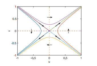
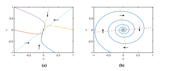
Now, to examine the possibility of traveling wave solutions, we look for a solution of the form $u(\xi, \tau)=U(\xi-c \tau), s(\xi, \tau)=S(\xi-c \tau)$, and find the system of ordinary differential equations
$$
\begin{aligned}
0 &=\frac{d^{2} U}{d \zeta^{2}}+c \frac{d U}{d \zeta}+U S \
0 &=\delta \frac{d^{2} S}{d \zeta^{2}}+c \frac{d S}{d \zeta}-U S
\end{aligned}
$$

数学代写|微分方程代写differential equation代考|Spread of Rabies—SIR with Diffusion

It has been observed in England that rabid foxes tend to travel across much larger distances than rabies free animals. This observation has led to consideration of the spread of an infectious disease where the infected animals diffuse, but susceptible animals do not [51]. For this we consider the standard SIR disease dynamics
$$
S+I \stackrel{\alpha}{\longrightarrow} 2 I, \quad I \stackrel{\beta}{\longrightarrow} R,
$$
where $S$ represents the susceptible population, $I$ represents the infected population, and $R$ represents the recovered (or removed) population. The corresponding differential equations are
$$
\begin{aligned}
&\frac{\partial s}{\partial t}=-\alpha s i \
&\frac{\partial i}{\partial t}=\alpha s i-\beta i+D \frac{\partial^{2} i}{\partial x^{2}} .
\end{aligned}
$$
Introducing dimensionless variables $\sigma=\frac{s}{S_{0}}, u=\frac{i}{S_{0}}, t=\frac{\tau}{\alpha S_{0}}$, and $x=\sqrt{\frac{D}{\alpha S_{0}}} \xi$, we find the dimensionless equations
$$
\begin{aligned}
&\frac{\partial \sigma}{\partial \tau}=-\sigma u, \
&\frac{\partial u}{\partial \tau}=\sigma u-\eta u+\frac{\partial^{2} u}{\partial \xi^{2}},
\end{aligned}
$$
depending on the single parameter $\eta=\frac{\beta}{\alpha S_{0}}=\frac{1}{R_{0}}$. A simulation of these equations is shown in Figure 6.15, and was computed using the Matlab code $\mathrm{CN}_{\text {_diffusion_SIR.m. }}$
As you can see from this figure, an initial amount of $u$ grows and spreads as a traveling wave, leading to a permanent decrease in the amount of $\sigma$, while the spreading bulge of $u$ is only temporary, as recovery eventually restores $u$ to zero. We would like to determine how fast this infection spreads and how much of the initial susceptible population is affected by it.

微分方程代考

数学代写|微分方程代写differential equation代考|Growth with a Carrying Capacity—Fisher’s Equation

现在我们考虑一个扩散和繁殖的人口，其中存在人口规模依赖性死亡。我们可以用两个反应来表示这一点

在⟶一个2在,在+在⟶b在.
对于这些反应，守恒方程为

∂在∂吨=D∂2在∂X2+一个在−b在2.
通常以稍微不同的形式写出这个方程

∂在∂吨=D∂2在∂X2+一个在(1−在ķ),
在哪里ķ=一个b称为承载能力。通过设置重新调整变量在= 一个b在=ķ在,吨=τ一个， 和X=D一个X，方程简化为

∂在∂τ=∂2在∂X2+在−在2
没有自由参数。
该方程的第二个推导与 SIR 流行病模型有关。这里我们假设有两个种群，表示为小号和我，分别代表易感人群和感染人群。易感个体可以通过与另一个受感染个体接触而被感染，但不可能从感染中恢复；受感染的个体具有永久传染性。这个过程可以用反应来表示

小号+我⟶一个2我这两个种群的守恒方程是

∂s∂吨=Ds∂2s∂X2−一个s一世,∂一世∂吨=D一世∂2一世∂X2+一个s一世.
在假设两个群体的扩散系数相同的情况下，Ds=D一世， 数量s+一世满足扩散方程，因此具有稳定、恒定的解s+一世=小号0. 有了这个守恒量，方程为一世变成

∂一世∂吨=D一世∂2一世∂X2+一个一世(小号0−一世)
通过设置重新调整变量一世=小号0在,吨=τ一个小号0,X=D一世一个小号0X，方程简化为(6.30).

数学代写|微分方程代写differential equation代考|Resource Consumption

现在考虑生物体（例如细菌）消耗资源基质（例如葡萄糖）的情况，而葡萄糖的供应是有限的。例如，假设细菌在 Petrie 培养皿上的琼脂凝胶上生长。描述这个的反应是

在+小号⟶一个2在.
上的单位在和小号是这样的，一个单位小号转换为一个单位在. 我们假设葡萄糖和细菌都通过扩散移动。因此，描述这种演变的微分方程（在一个空间维度上）是

∂在∂吨=D在∂2在∂X2+一个在s ∂s∂吨=DG∂2s∂X2−一个在s
在哪里s表示资源底物（即葡萄糖）的浓度。该方程组的数值模拟如图 6.13 所示。该仿真的 Matlab 代码名为 CN_diffusion_gluc_micro_X.m。该模拟再次表明应该存在行波解决方案。分析的第一步是通过引入缩放变量来简化方程吨=τ一个,X=D在一个X，据此方程变为

∂在∂τ=∂2在∂X2+在s ∂s∂τ=d∂2s∂X2−在s
在哪里d=DGD在.
现在，为了检验行波解的可能性，我们寻找以下形式的解在(X,τ)=在(X−Cτ),s(X,τ)=小号(X−Cτ), 并找到常微分方程组

0=d2在dG2+Cd在dG+在小号 0=dd2小号dG2+Cd小号dG−在小号

数学代写|微分方程代写differential equation代考|Spread of Rabies—SIR with Diffusion

在英格兰已经观察到，与没有狂犬病的动物相比，患有狂犬病的狐狸往往会穿越更远的距离。这一观察结果导致人们考虑传染病的传播，其中受感染的动物扩散，但易感动物没有[51]。为此，我们考虑标准 SIR 疾病动态

小号+我⟶一个2我,我⟶bR,
在哪里小号代表易感人群，我代表受感染的人群，并且R代表恢复（或删除）的人口。对应的微分方程是

∂s∂吨=−一个s一世 ∂一世∂吨=一个s一世−b一世+D∂2一世∂X2.
引入无量纲变量σ=s小号0,在=一世小号0,吨=τ一个小号0， 和X=D一个小号0X，我们找到无量纲方程

∂σ∂τ=−σ在, ∂在∂τ=σ在−这在+∂2在∂X2,
取决于单个参数这=b一个小号0=1R0. 这些方程的模拟如图 6.15 所示，并使用 Matlab 代码计算Cñ_diffusion_SIR.m。 
从图中可以看出，初始数量为在以行波的形式增长和传播，导致数量永久减少σ，而膨胀的膨胀在只是暂时的，因为恢复最终会恢复在为零。我们想确定这种感染的传播速度以及有多少最初的易感人群受到它的影响。

统计代写请认准statistics-lab™. statistics-lab™为您的留学生涯保驾护航。

金融工程代写

金融工程是使用数学技术来解决金融问题。金融工程使用计算机科学、统计学、经济学和应用数学领域的工具和知识来解决当前的金融问题，以及设计新的和创新的金融产品。

非参数统计代写

非参数统计指的是一种统计方法，其中不假设数据来自于由少数参数决定的规定模型；这种模型的例子包括正态分布模型和线性回归模型。

广义线性模型代考

广义线性模型（GLM）归属统计学领域，是一种应用灵活的线性回归模型。该模型允许因变量的偏差分布有除了正态分布之外的其它分布。

术语 广义线性模型（GLM）通常是指给定连续和/或分类预测因素的连续响应变量的常规线性回归模型。它包括多元线性回归，以及方差分析和方差分析（仅含固定效应）。

有限元方法代写

有限元方法（FEM）是一种流行的方法，用于数值解决工程和数学建模中出现的微分方程。典型的问题领域包括结构分析、传热、流体流动、质量运输和电磁势等传统领域。

有限元是一种通用的数值方法，用于解决两个或三个空间变量的偏微分方程（即一些边界值问题）。为了解决一个问题，有限元将一个大系统细分为更小、更简单的部分，称为有限元。这是通过在空间维度上的特定空间离散化来实现的，它是通过构建对象的网格来实现的：用于求解的数值域，它有有限数量的点。边界值问题的有限元方法表述最终导致一个代数方程组。该方法在域上对未知函数进行逼近。[1] 然后将模拟这些有限元的简单方程组合成一个更大的方程系统，以模拟整个问题。然后，有限元通过变化微积分使相关的误差函数最小化来逼近一个解决方案。

tatistics-lab作为专业的留学生服务机构，多年来已为美国、英国、加拿大、澳洲等留学热门地的学生提供专业的学术服务，包括但不限于Essay代写，Assignment代写，Dissertation代写，Report代写，小组作业代写，Proposal代写，Paper代写，Presentation代写，计算机作业代写，论文修改和润色，网课代做，exam代考等等。写作范围涵盖高中，本科，研究生等海外留学全阶段，辐射金融，经济学，会计学，审计学，管理学等全球99%专业科目。写作团队既有专业英语母语作者，也有海外名校硕博留学生，每位写作老师都拥有过硬的语言能力，专业的学科背景和学术写作经验。我们承诺100%原创，100%专业，100%准时，100%满意。

随机分析代写

随机微积分是数学的一个分支，对随机过程进行操作。它允许为随机过程的积分定义一个关于随机过程的一致的积分理论。这个领域是由日本数学家伊藤清在第二次世界大战期间创建并开始的。

时间序列分析代写

随机过程，是依赖于参数的一组随机变量的全体，参数通常是时间。 随机变量是随机现象的数量表现，其时间序列是一组按照时间发生先后顺序进行排列的数据点序列。通常一组时间序列的时间间隔为一恒定值（如1秒，5分钟，12小时，7天，1年），因此时间序列可以作为离散时间数据进行分析处理。研究时间序列数据的意义在于现实中，往往需要研究某个事物其随时间发展变化的规律。这就需要通过研究该事物过去发展的历史记录，以得到其自身发展的规律。

回归分析代写

多元回归分析渐进（Multiple Regression Analysis Asymptotics）属于计量经济学领域，主要是一种数学上的统计分析方法，可以分析复杂情况下各影响因素的数学关系，在自然科学、社会和经济学等多个领域内应用广泛。

MATLAB代写

MATLAB 是一种用于技术计算的高性能语言。它将计算、可视化和编程集成在一个易于使用的环境中，其中问题和解决方案以熟悉的数学符号表示。典型用途包括：数学和计算算法开发建模、仿真和原型制作数据分析、探索和可视化科学和工程图形应用程序开发，包括图形用户界面构建MATLAB 是一个交互式系统，其基本数据元素是一个不需要维度的数组。这使您可以解决许多技术计算问题，尤其是那些具有矩阵和向量公式的问题，而只需用 C 或 Fortran 等标量非交互式语言编写程序所需的时间的一小部分。MATLAB 名称代表矩阵实验室。MATLAB 最初的编写目的是提供对由 LINPACK 和 EISPACK 项目开发的矩阵软件的轻松访问，这两个项目共同代表了矩阵计算软件的最新技术。MATLAB 经过多年的发展，得到了许多用户的投入。在大学环境中，它是数学、工程和科学入门和高级课程的标准教学工具。在工业领域，MATLAB 是高效研究、开发和分析的首选工具。MATLAB 具有一系列称为工具箱的特定于应用程序的解决方案。对于大多数 MATLAB 用户来说非常重要，工具箱允许您学习和应用专业技术。工具箱是 MATLAB 函数（M 文件）的综合集合，可扩展 MATLAB 环境以解决特定类别的问题。可用工具箱的领域包括信号处理、控制系统、神经网络、模糊逻辑、小波、仿真等。

R语言代写	问卷设计与分析代写
PYTHON代写	回归分析与线性模型代写
MATLAB代写	方差分析与试验设计代写
STATA代写	机器学习/统计学习代写
SPSS代写	计量经济学代写
EVIEWS代写	时间序列分析代写
EXCEL代写	深度学习代写
SQL代写	各种数据建模与可视化代写

如果你也在 怎样代写微分方程differential equation这个学科遇到相关的难题，请随时右上角联系我们的24/7代写客服。

微分方程（ODE）是一个微分方程，包含一个或多个独立变量的函数以及这些函数的导数。术语普通是与术语偏微分方程相对应的，后者可能与一个以上的独立变量有关。

statistics-lab™ 为您的留学生涯保驾护航 在代写微分方程differential equation方面已经树立了自己的口碑, 保证靠谱, 高质且原创的统计Statistics代写服务。我们的专家在代写微分方程differential equation代写方面经验极为丰富，各种代写微分方程differential equation相关的作业也就用不着说。

我们提供的微分方程differential equation及其相关学科的代写，服务范围广, 其中包括但不限于:

• Statistical Inference 统计推断
• Statistical Computing 统计计算
• Advanced Probability Theory 高等概率论
• Advanced Mathematical Statistics 高等数理统计学
• (Generalized) Linear Models 广义线性模型
• Statistical Machine Learning 统计机器学习
• Longitudinal Data Analysis 纵向数据分析
• Foundations of Data Science 数据科学基础

数学代写|微分方程代写differential equation代考|Numerical Methods

The first method to numerically simulate the diffusion equation is one that we have already used, namely the method of lines. With this method, we discretize the spatial region into a grid with points at $x_{j}=j \Delta x$, $j=0,1, \ldots, N$, and then write the diffusion equation approximately as the system of ordinary differential equations
$$
\frac{d u_{j}}{d t}=\frac{D}{\Delta x^{2}}\left(u_{j+1}-2 u_{j}+u_{j-1}\right) .
$$
At the endpoints, take the equations to be
$$
\frac{d u_{0}}{d t}=\frac{2 D}{\Delta x^{2}}\left(u_{1}-u_{0}\right), \quad \frac{d u_{N}}{d t}=\frac{2 D}{\Delta x^{2}}\left(u_{j-1}-u_{N}\right) .
$$
This choice follows from the approximation to the derivative of $u,\left.\frac{\partial u}{\partial x}\right|{x=j \Delta x} \approx \frac{u{j+1}-u_{j-1}}{2 \Delta x}$, so at the boundaries the zero derivative (Neumann) boundary condition implies that $u_{-1}=u_{1}$, and $u_{N+1}=u_{N-1}$. (The points at $j=-1$ and $j=N+1$ are called ghost points and are useful for this calculation, but are never actually computed.)

This system of equations is then simulated using a numerical ordinary differential equation solver. The Matlab code for this for Neumann or Robin boundary conditions is titled Diffusion_NK_via_MUL.m and for Dirichlet boundary conditions is titled Diffusion_Dirichlet_via_MOL.m.

It is convenient for future discussions to represent $u(j \Delta x, t)$ as a vector $\mathbf{u}(t)=\left(u_{j}\right)$, and then to rewrite (5.37) using vector/matrix notation as
$$
\frac{d \mathbf{u}}{d t}=\frac{D}{\Delta x^{2}} A \mathbf{u}
$$
where the matrix $A$ has diagonal elements $-2$, and first upper and lower off-diagonal elements 1 , except the first element of the upper diagonal and last element of the lower diagonal are both 2, i.e.,
$$
A=\left(\begin{array}{ccccc}
-2 & 2 & 0 & \cdots & 0 \
1 & -2 & 1 & 0 & \cdots \
& & \vdots & & \
0 & \cdots & 1 & -2 & 1 \
0 & \cdots & 0 & 2 & -2
\end{array}\right)
$$

数学代写|微分方程代写differential equation代考|Other Boundary Conditions

Everything discussed in the previous section was for Neumann boundary conditions. However, the only difference for the numerical methods with different boundary conditions is with the definition of the corner entries of the matrix $A$. For homogeneous Robin boundary conditions (5.23), we write the approximations
$$
D\left(\frac{u_{1}-u_{-1}}{2 \Delta x}\right)=\delta u_{0}, \quad-D\left(\frac{u_{N+1}-u_{N-1}}{2 \Delta x}\right)=\delta u_{N}
$$
which when substituted into the finite difference approximation of the diffusion equation (5.37) yields
$$
\frac{d u_{0}}{d t}=\frac{D}{\Delta x^{2}}\left(2 u_{1}-2\left(1+\frac{\delta \Delta x}{D}\right) u_{0}\right)
$$
$$
\frac{d u_{N}}{d t}=\frac{D}{\Delta x^{2}}\left(2\left(-1-\frac{\delta \Delta x}{D}\right) u_{N}+2 u_{N-1}\right) .
$$
This implies that the matrix $A$ in (5.40) needs to be modified slightly to have first and last diagonal elements
$$
A_{1,1}=-2-2 \frac{\delta \Delta x}{D}, \quad A_{N+1, N+1}=-2-2 \frac{\delta \Delta x}{D}
$$
For homogeneous Dirichlet boundary conditions, the unknown variables are $u_{j}$, $j=1,2, \ldots, u_{N-1}$, (two less than for Neumann and Robin conditions) and the finite difference approximation (5.37) for $u_{1}$ and $u_{N ~}$
$$
\text { (5.56) } \frac{d u_{1}}{d t}=\frac{D}{\Delta x^{2}}\left(u_{2}-2 u_{1}\right), \quad \frac{d u_{N-1}}{d t}=\frac{D}{\Delta x^{2}}\left(-2 u_{N-1}+u_{N-2}\right)
$$
(since $u_{0}=u_{N}=0$ ) and consequently, the matrix $A$ (which is now an $N-1 \times N-1$ matrix) is
$$
A=\left(\begin{array}{ccccc}
-2 & 1 & 0 & \cdots & 0 \
1 & -2 & 1 & 0 & \cdots \
& & \vdots & & \
0 & \cdots & 1 & -2 & 1 \
0 & \cdots & 0 & 1 & -2
\end{array}\right)
$$
For Dirichlet boundary conditions, the Matlab codes are FEuler_diffusion_dirichlet.m, BEuler_diffusion_Dirichlet.m, and CN_diffusion_Dirichlet.m for forward Euler, backward Euler, and Crank-Nicolson methods, respectively.

数学代写|微分方程代写differential equation代考|Birth-Death with Diffusion

Suppose that there is some population or chemical species $U$ that diffuses on an infinite domain and experiences either decay, as in
$$
U \stackrel{\alpha}{\longrightarrow} \emptyset,
$$
or birth via asexual duplication as in
$$
U \stackrel{\alpha}{\longrightarrow} 2 U
$$
Setting $u=[U]$, the equation describing the evolution of this population is
$$
\frac{\partial u}{\partial t}=D \frac{\partial^{2} u}{\partial x^{2}}+\sigma \alpha u,
$$
where $\alpha>0, \sigma=-1$ for decay, and $\sigma=1$ for growth.
As an example, suppose that signaling molecules are produced at some point, and that the target of the signal is some distance away. Specifically, many copies of a transcription factor may be made when only one is needed to activate transcription of a gene. What percentage, if any, of the signaling molecules reach the target before they degrade? Roughly $10^{8}$ sperm cells are initially released to reach the oocyte in human fertilization when only one is required. What are the consequences of releasing fewer sperm cells? This could also be a model to determine the distribution of seeds falling

to the ground after release from a seed pod into the air. This seed dispersal problem is discussed more in Chapter $13 .$

Let’s begin our study of this problem of diffusion with decay with a stochastic simulation. To do this, we modify the algorithm from Chapter 4 that simulates diffusing particles to account for the possibility of degradation. At each time step, the particle can move or degrade, and if it degrades, its motion is terminated. The Matlab code to implement this is titled decay_probability.m, and the result of a simulation is shown in Figure 6.1. What we see in this figure may be a bit surprising; the distribution of decay position is clearly not a Gaussian distribution. But what is it?

微分方程代考

数学代写|微分方程代写differential equation代考|Numerical Methods

第一种数值模拟扩散方程的方法是我们已经使用过的方法，即线法。使用这种方法，我们将空间区域离散化为一个网格，其中的点位于Xj=jΔX, j=0,1,…,ñ，然后将扩散方程近似写为常微分方程组

d在jd吨=DΔX2(在j+1−2在j+在j−1).
在端点处，取方程为

d在0d吨=2DΔX2(在1−在0),d在ñd吨=2DΔX2(在j−1−在ñ).
这种选择是从近似到导数得出的在,∂在∂X|X=jΔX≈在j+1−在j−12ΔX，因此在边界处，零导数 (Neumann) 边界条件意味着在−1=在1， 和在ñ+1=在ñ−1. （点在j=−1和j=ñ+1被称为鬼点，对这种计算很有用，但实际上从未计算过。）

然后使用数值常微分方程求解器模拟该方程组。用于 Neumann 或 Robin 边界条件的 Matlab 代码标题为 Diffusion_NK_via_MUL.m，Dirichlet 边界条件的标题为 Diffusion_Dirichlet_via_MOL.m。

方便以后讨论代表在(jΔX,吨)作为向量在(吨)=(在j)，然后使用向量/矩阵表示法将 (5.37) 重写为

d在d吨=DΔX2一个在
矩阵在哪里一个有对角线元素−2, 和第一个上和下非对角元素 1 ，除了上对角线的第一个元素和下对角线的最后一个元素都是 2，即

一个=(−220⋯0 1−210⋯ ⋮ 0⋯1−21 0⋯02−2)

数学代写|微分方程代写differential equation代考|Other Boundary Conditions

上一节讨论的所有内容都是针对 Neumann 边界条件的。然而，具有不同边界条件的数值方法的唯一区别是矩阵的角条目的定义一个. 对于齐次 Robin 边界条件 (5.23)，我们写出近似值

D(在1−在−12ΔX)=d在0,−D(在ñ+1−在ñ−12ΔX)=d在ñ
当代入扩散方程（5.37）的有限差分近似时，得到

d在0d吨=DΔX2(2在1−2(1+dΔXD)在0)

d在ñd吨=DΔX2(2(−1−dΔXD)在ñ+2在ñ−1).
这意味着矩阵一个在（5.40）中需要稍微修改以具有第一个和最后一个对角线元素

一个1,1=−2−2dΔXD,一个ñ+1,ñ+1=−2−2dΔXD
对于齐次狄利克雷边界条件，未知变量为在j, j=1,2,…,在ñ−1,（Neumann 和 Robin 条件下小于两个）和有限差分近似 (5.37)在1和在ñ 

 (5.56) d在1d吨=DΔX2(在2−2在1),d在ñ−1d吨=DΔX2(−2在ñ−1+在ñ−2)
（自从在0=在ñ=0)，因此，矩阵一个（现在是一个ñ−1×ñ−1矩阵）是

一个=(−210⋯0 1−210⋯ ⋮ 0⋯1−21 0⋯01−2)
对于 Dirichlet 边界条件，Matlab 代码分别为 FEuler_diffusion_dirichlet.m、BEuler_diffusion_Dirichlet.m 和 CN_diffusion_Dirichlet.m，用于正向 Euler、反向 Euler 和 Crank-Nicolson 方法。

数学代写|微分方程代写differential equation代考|Birth-Death with Diffusion

假设有一些种群或化学物种在它扩散到无限的领域并经历衰变，如

在⟶一个∅,
或通过无性复制出生，如

在⟶一个2在
环境在=[在]，描述这个种群进化的方程是

∂在∂吨=D∂2在∂X2+σ一个在,
在哪里一个>0,σ=−1腐烂，和σ=1为了成长。
举个例子，假设信号分子是在某个点产生的，并且信号的目标距离很远。具体而言，当只需要一个来激活基因的转录时，可能会产生许多拷贝的转录因子。信号分子在降解之前达到目标的百分比（如果有的话）？大致108当只需要一个时，精子细胞最初会在人类受精过程中被释放以到达卵母细胞。释放更少的精子细胞会有什么后果？这也可以作为确定落下种子分布的模型

从种子荚释放到空中后落到地面上。种子传播问题将在本章中详细讨论13.

让我们通过随机模拟开始研究这个带有衰减的扩散问题。为此，我们修改了第 4 章中模拟扩散粒子的算法，以考虑降解的可能性。在每个时间步，粒子可以移动或退化，如果退化，它的运动就会终止。实现这一点的 Matlab 代码名为 decay_probability.m，仿真结果如图 6.1 所示。我们在这张图中看到的可能有点令人惊讶；衰减位置的分布显然不是高斯分布。但它是什么？

统计代写请认准statistics-lab™. statistics-lab™为您的留学生涯保驾护航。

金融工程代写

金融工程是使用数学技术来解决金融问题。金融工程使用计算机科学、统计学、经济学和应用数学领域的工具和知识来解决当前的金融问题，以及设计新的和创新的金融产品。

非参数统计代写

非参数统计指的是一种统计方法，其中不假设数据来自于由少数参数决定的规定模型；这种模型的例子包括正态分布模型和线性回归模型。

广义线性模型代考

广义线性模型（GLM）归属统计学领域，是一种应用灵活的线性回归模型。该模型允许因变量的偏差分布有除了正态分布之外的其它分布。

术语 广义线性模型（GLM）通常是指给定连续和/或分类预测因素的连续响应变量的常规线性回归模型。它包括多元线性回归，以及方差分析和方差分析（仅含固定效应）。

有限元方法代写

有限元方法（FEM）是一种流行的方法，用于数值解决工程和数学建模中出现的微分方程。典型的问题领域包括结构分析、传热、流体流动、质量运输和电磁势等传统领域。

有限元是一种通用的数值方法，用于解决两个或三个空间变量的偏微分方程（即一些边界值问题）。为了解决一个问题，有限元将一个大系统细分为更小、更简单的部分，称为有限元。这是通过在空间维度上的特定空间离散化来实现的，它是通过构建对象的网格来实现的：用于求解的数值域，它有有限数量的点。边界值问题的有限元方法表述最终导致一个代数方程组。该方法在域上对未知函数进行逼近。[1] 然后将模拟这些有限元的简单方程组合成一个更大的方程系统，以模拟整个问题。然后，有限元通过变化微积分使相关的误差函数最小化来逼近一个解决方案。

tatistics-lab作为专业的留学生服务机构，多年来已为美国、英国、加拿大、澳洲等留学热门地的学生提供专业的学术服务，包括但不限于Essay代写，Assignment代写，Dissertation代写，Report代写，小组作业代写，Proposal代写，Paper代写，Presentation代写，计算机作业代写，论文修改和润色，网课代做，exam代考等等。写作范围涵盖高中，本科，研究生等海外留学全阶段，辐射金融，经济学，会计学，审计学，管理学等全球99%专业科目。写作团队既有专业英语母语作者，也有海外名校硕博留学生，每位写作老师都拥有过硬的语言能力，专业的学科背景和学术写作经验。我们承诺100%原创，100%专业，100%准时，100%满意。

随机分析代写

随机微积分是数学的一个分支，对随机过程进行操作。它允许为随机过程的积分定义一个关于随机过程的一致的积分理论。这个领域是由日本数学家伊藤清在第二次世界大战期间创建并开始的。

时间序列分析代写

随机过程，是依赖于参数的一组随机变量的全体，参数通常是时间。 随机变量是随机现象的数量表现，其时间序列是一组按照时间发生先后顺序进行排列的数据点序列。通常一组时间序列的时间间隔为一恒定值（如1秒，5分钟，12小时，7天，1年），因此时间序列可以作为离散时间数据进行分析处理。研究时间序列数据的意义在于现实中，往往需要研究某个事物其随时间发展变化的规律。这就需要通过研究该事物过去发展的历史记录，以得到其自身发展的规律。

回归分析代写

多元回归分析渐进（Multiple Regression Analysis Asymptotics）属于计量经济学领域，主要是一种数学上的统计分析方法，可以分析复杂情况下各影响因素的数学关系，在自然科学、社会和经济学等多个领域内应用广泛。

MATLAB代写

MATLAB 是一种用于技术计算的高性能语言。它将计算、可视化和编程集成在一个易于使用的环境中，其中问题和解决方案以熟悉的数学符号表示。典型用途包括：数学和计算算法开发建模、仿真和原型制作数据分析、探索和可视化科学和工程图形应用程序开发，包括图形用户界面构建MATLAB 是一个交互式系统，其基本数据元素是一个不需要维度的数组。这使您可以解决许多技术计算问题，尤其是那些具有矩阵和向量公式的问题，而只需用 C 或 Fortran 等标量非交互式语言编写程序所需的时间的一小部分。MATLAB 名称代表矩阵实验室。MATLAB 最初的编写目的是提供对由 LINPACK 和 EISPACK 项目开发的矩阵软件的轻松访问，这两个项目共同代表了矩阵计算软件的最新技术。MATLAB 经过多年的发展，得到了许多用户的投入。在大学环境中，它是数学、工程和科学入门和高级课程的标准教学工具。在工业领域，MATLAB 是高效研究、开发和分析的首选工具。MATLAB 具有一系列称为工具箱的特定于应用程序的解决方案。对于大多数 MATLAB 用户来说非常重要，工具箱允许您学习和应用专业技术。工具箱是 MATLAB 函数（M 文件）的综合集合，可扩展 MATLAB 环境以解决特定类别的问题。可用工具箱的领域包括信号处理、控制系统、神经网络、模糊逻辑、小波、仿真等。

R语言代写	问卷设计与分析代写
PYTHON代写	回归分析与线性模型代写
MATLAB代写	方差分析与试验设计代写
STATA代写	机器学习/统计学习代写
SPSS代写	计量经济学代写
EVIEWS代写	时间序列分析代写
EXCEL代写	深度学习代写
SQL代写	各种数据建模与可视化代写

如果你也在 怎样代写微分方程differential equation这个学科遇到相关的难题，请随时右上角联系我们的24/7代写客服。

微分方程（ODE）是一个微分方程，包含一个或多个独立变量的函数以及这些函数的导数。术语普通是与术语偏微分方程相对应的，后者可能与一个以上的独立变量有关。

statistics-lab™ 为您的留学生涯保驾护航 在代写微分方程differential equation方面已经树立了自己的口碑, 保证靠谱, 高质且原创的统计Statistics代写服务。我们的专家在代写微分方程differential equation代写方面经验极为丰富，各种代写微分方程differential equation相关的作业也就用不着说。

我们提供的微分方程differential equation及其相关学科的代写，服务范围广, 其中包括但不限于:

• Statistical Inference 统计推断
• Statistical Computing 统计计算
• Advanced Probability Theory 高等概率论
• Advanced Mathematical Statistics 高等数理统计学
• (Generalized) Linear Models 广义线性模型
• Statistical Machine Learning 统计机器学习
• Longitudinal Data Analysis 纵向数据分析
• Foundations of Data Science 数据科学基础

数学代写|微分方程代写differential equation代考|With Boundary Conditions

Up to this point we have not discussed much about boundary conditions, but these can be avoided no longer. As the name implies, a boundary condition is a condition on the solution at the boundary of the domain of interest. In general, one needs one condition for every derivative that appears in the equation. Thus, for example, for a differential equation that describes the time evolution of some object with an equation of the form $u_{t}=f(u, t)$, one needs one initial condition to specify $u\left(t_{0}\right)$, where $t_{0}$ is the start time. On the other hand for a differential equation that can be written as $u_{x x}=g\left(u, u_{x}, x\right)$, one needs two conditions at the boundaries in order to specify $u$ completely. Thus, for the diffusion equation on a finite domain, one needs to specify an initial condition at $t=0$ for all values of $x$ in the domain, and two boundary conditions at the ends of the spatial domain. For a one dimensional spatial domain there are four possibilities:

• Dirichlet condition is when the value of the unknown $u$ is specified at the boundary. If $u$ is a probability, the condition $u=0$ is said to be an absorbing boundary condition, because a particle that crosses the boundary disappears and cannot re-enter the domain.
• Neumann condition is when the flux of the unknown $u$ across the boundary is specified. In a biological context, the flux across a boundary is zero if the boundary is impermeable to the particles, and is often called a no-flux condition. If $u$ is a probability, $\nabla u \cdot \mathbf{n}=0$ is called a reflecting boundary condition.
• Robin condition is a weighted combination of Dirichlet and Neumann boundary conditions, typically of the form $D \nabla u \cdot \mathbf{n}+a u=b$ and is often appropriate when the diffusing species can undergo a chemical reaction at the boundary, or, as we see below, when the species can diffuse across a porous boundary.
• Periodic conditions apply when the one dimensional domain is actually a closed loop of length $L$, with the point at $x=0$ the same as the point at $x=L$. In this case, one requires that the function $u$ and its derivative be continuous at the “boundary”.

数学代写|微分方程代写differential equation代考|At Steady State

Before we move on to solve the diffusion equation with different boundary conditions, it is worthwhile to gain some exposure to these by examining what happens when a diffusion process is at steady state. Steady state means that $u$ is not changing in time, i.e., $\frac{\partial u}{\partial t}=0$, so that the process is in equilibrium, but it does not mean that nothing is happening.

To illustrate, suppose $u$ is held fixed at $u=u_{0}$ at $x=0$ and $u=u_{L}$ at $x=L$. Then, the steady state solution satisfies $u_{x x}=0$, which implies that $u$ is a linear function satisfying the boundary conditions, i.e.,
$$
u(x)=u_{L} \frac{x}{L}+u_{0}\left(1-\frac{x}{L}\right) .
$$
To verify that something is happening, notice that the flux is
$$
J=-D u_{x}=\frac{D}{L}\left(u_{0}-u_{L}\right),
$$
which is not zero, unless $u_{L}=u_{0}$.

Suppose, instead, that the boundaries at $x=0$ and $x=L$ are porous membranes, with $u=u_{0}$ and $u=u_{L}$ just outside the domain, and the species $u$ can diffuse through the boundaries and therefore must satisfy the Robin boundary conditions
$$
\left.D u_{x}\right|{x=0}=\delta\left(u(0)-u{0}\right), \quad-\left.D u_{x}\right|{x=L}=\delta\left(u(L)-u{L}\right) .
$$
where $\delta>0$ represents the porosity of the boundary membrane, and $u(0), u(L)$ are the values of $u$ at the membrane just inside the domain. Notice what these conditions mean in words: the term $\delta\left(u(0)-u_{0}\right)$ is the diffusive flux of u across the membrane to the outside, and $\left.D u_{x}\right|{x=0}$ is the flux of $u$ out of the domain at $x=0$. Clearly these must match. Notice also the difference in the sign for these two conditions. This is because if $u(0)>u{0}$, the flux will be out of the domain to the left, i.e., negative (and because flux is the negative spatial derivative of $u, u$ must therefore have positive slope). If $u(L)>u_{L}$, the flux will be out of the domain to the right, i.e., positive (hence $u$ must have a negative slope). As before, $u$ is a linear function in the interior of the domain, and the requirement that it satisfy the two Robin boundary conditions yields that
$$
u(x)=\frac{1}{1+2 \Delta}\left(u_{L}-u_{0}\right) \frac{x}{L}+\frac{\Delta\left(u_{0}+u_{L}\right)+u_{0}}{1+2 \Delta}
$$
where $\Delta=\frac{D}{\delta L}$. Once again, the flux is nontrivial, being
$$
J=-D u_{x}=\frac{D}{1+2 \Delta} \frac{u_{0}-u_{L}}{L} .
$$
The quantity $D_{\text {eff }}=\frac{D}{1+2 \Delta}$ is the effective diffusion coefficient for this membrane bound medium, since the species must diffuse across both membranes and well as through the interior of the medium. Notice also the identity
$$
\frac{L}{D_{\text {eff }}}=\frac{1}{\delta}+\frac{L}{D}+\frac{1}{\delta}
$$
(What do you suspect the answer is if the two porosities are different? Can you verify this suspicion? See Exercise 5.5.) Clearly, in the limit that the porosity of the membrane $\delta \rightarrow \infty$, the problem reduces to the Dirichlet boundary condition with solution (5.22) (see Figure 5.2).

数学代写|微分方程代写differential equation代考|Separation of Variables

In biological applications, the most common boundary condition is the no-flux (homogeneous Neumann) condition, when particles are trapped inside a bounded domain, and this is where we begin our study of time dependent solutions of the diffusion equation on a bounded domain.

An important feature of the no-flux boundary condition is that the total amount of the quantity $u$ is conserved; this follows immediately from the conservation law as stated in (2.1). When solving any differential equation (in time) with constant coefficients, it is reasonable to try a solution that is exponential in time. For the diffusion

equation, we try a solution of the form
$$
u(x, t)=U(x) \exp (\lambda t),
$$
and upon substituting into the diffusion equation (3.2), we find
$$
D \frac{d^{2} U}{d x^{2}}-\lambda U=0 .
$$
This equation must be solved subject to the no-flux boundary condition $U^{\prime}(0)=$ $U^{\prime}(L)=0 .$

There are an infinite number of possible solutions, but they are all of the same form, namely
$$
U_{n}(x)=a_{n} \cos \left(\frac{n \pi x}{L}\right),
$$
with the important restriction that
$$
\lambda=\lambda_{n} \equiv-\frac{n^{2} \pi^{2} D}{L^{2}},
$$
with $n=0,1,2, \ldots$
Since there are an infinite number of possible solutions, and the diffusion equation is linear, the fully general solution is an arbitrary linear combination of the possible solutions, namely
$$
u(x, t)=\sum_{n=0}^{\infty} a_{n} \exp \left(-\frac{D n^{2} \pi^{2} t}{L^{2}}\right) \cos \left(\frac{n \pi x}{L}\right)
$$

微分方程代考

数学代写|微分方程代写differential equation代考|With Boundary Conditions

到目前为止，我们还没有过多地讨论边界条件，但这些已经无法避免了。顾名思义，边界条件是对感兴趣域边界处的解的条件。一般来说，方程中出现的每一个导数都需要一个条件。因此，例如，对于描述某个对象的时间演化的微分方程，其方程为在吨=F(在,吨), 需要一个初始条件来指定在(吨0)， 在哪里吨0是开始时间。另一方面，对于可以写成的微分方程在XX=G(在,在X,X), 在边界处需要两个条件才能指定在完全地。因此，对于有限域上的扩散方程，需要指定初始条件吨=0对于所有值X在域中，在空间域的末端有两个边界条件。对于一维空间域，有四种可能性：

• 狄利克雷条件是当未知值在在边界处指定。如果在是概率，条件在=0被称为吸收边界条件，因为穿过边界的粒子消失并且不能重新进入域。
• 诺伊曼条件是当未知的通量在指定跨界。在生物学背景下，如果边界对粒子是不可渗透的，则跨边界的通量为零，并且通常称为无通量条件。如果在是概率，∇在⋅n=0称为反射边界条件。
• Robin 条件是 Dirichlet 和 Neumann 边界条件的加权组合，通常形式为D∇在⋅n+一个在=b当扩散物质可以在边界发生化学反应时，或者正如我们在下面看到的，当物质可以扩散穿过多孔边界时，通常是合适的。
• 当一维域实际上是一个长度的闭环时，周期性条件适用大号, 点在X=0与点相同X=大号. 在这种情况下，需要函数在并且它的导数在“边界”处是连续的。

数学代写|微分方程代写differential equation代考|At Steady State

在我们继续求解具有不同边界条件的扩散方程之前，有必要通过检查扩散过程处于稳态时发生的情况来了解这些情况。稳定状态意味着在不随时间变化，即∂在∂吨=0，因此过程处于平衡状态，但这并不意味着什么都没有发生。

为了说明，假设在固定在在=在0在X=0和在=在大号在X=大号. 那么稳态解满足在XX=0，这意味着在是满足边界条件的线性函数，即

在(X)=在大号X大号+在0(1−X大号).
要验证某事正在发生，请注意通量是

Ĵ=−D在X=D大号(在0−在大号),
这不是零，除非在大号=在0.

相反，假设边界在X=0和X=大号是多孔膜，具有在=在0和在=在大号就在领域之外，物种在可以通过边界扩散，因此必须满足 Robin 边界条件

D在X|X=0=d(在(0)−在0),−D在X|X=大号=d(在(大号)−在大号).
在哪里d>0表示边界膜的孔隙率，并且在(0),在(大号)是的值在在域内的膜上。请注意这些条件在文字中的含义：术语d(在(0)−在0)是 u 穿过膜到外部的扩散通量，并且D在X|X=0是通量在在域外X=0. 显然，这些必须匹配。还要注意这两个条件的符号差异。这是因为如果在(0)>在0，通量将在左侧的域外，即负（并且因为通量是负空间导数在,在因此必须具有正斜率）。如果在(大号)>在大号，通量将在域外向右，即正（因此在必须有一个负斜率）。和以前一样，在是域内部的线性函数，并且它满足两个 Robin 边界条件的要求产生

在(X)=11+2Δ(在大号−在0)X大号+Δ(在0+在大号)+在01+2Δ
在哪里Δ=Dd大号. 再一次，通量是不平凡的，即

Ĵ=−D在X=D1+2Δ在0−在大号大号.
数量D效果 =D1+2Δ是这种膜结合介质的有效扩散系数，因为物质必须扩散穿过两个膜并穿过介质内部。还要注意身份

大号D效果 =1d+大号D+1d
（如果两个孔隙率不同，你怀疑答案是什么？你能证实这个怀疑吗？见习题 5.5。）显然，在膜孔隙率的极限内d→∞，问题归结为狄利克雷边界条件，解为 (5.22)（见图 5.2）。

数学代写|微分方程代写differential equation代考|Separation of Variables

在生物应用中，最常见的边界条件是无通量（齐次诺依曼）条件，当粒子被困在有界域内时，我们开始研究有界域上扩散方程的时间相关解。

无通量边界条件的一个重要特征是数量的总量在是保守的；这直接来自 (2.1) 中所述的守恒定律。在求解任何具有常数系数的微分方程（时间）时，尝试时间上的指数解是合理的。对于扩散

方程，我们尝试以下形式的解

在(X,吨)=在(X)经验⁡(λ吨),
并代入扩散方程（3.2），我们发现

Dd2在dX2−λ在=0.
该方程必须在无通量边界条件下求解在′(0)= 在′(大号)=0.

有无数种可能的解，但它们的形式都是一样的，即

在n(X)=一个n因⁡(n圆周率X大号),
有一个重要的限制，即

λ=λn≡−n2圆周率2D大号2,
和n=0,1,2,…
由于有无限多的可能解，并且扩散方程是线性的，所以完全一般解是可能解的任意线性组合，即

在(X,吨)=∑n=0∞一个n经验⁡(−Dn2圆周率2吨大号2)因⁡(n圆周率X大号)

统计代写请认准statistics-lab™. statistics-lab™为您的留学生涯保驾护航。

金融工程代写

金融工程是使用数学技术来解决金融问题。金融工程使用计算机科学、统计学、经济学和应用数学领域的工具和知识来解决当前的金融问题，以及设计新的和创新的金融产品。

非参数统计代写

非参数统计指的是一种统计方法，其中不假设数据来自于由少数参数决定的规定模型；这种模型的例子包括正态分布模型和线性回归模型。

广义线性模型代考

广义线性模型（GLM）归属统计学领域，是一种应用灵活的线性回归模型。该模型允许因变量的偏差分布有除了正态分布之外的其它分布。

术语 广义线性模型（GLM）通常是指给定连续和/或分类预测因素的连续响应变量的常规线性回归模型。它包括多元线性回归，以及方差分析和方差分析（仅含固定效应）。

有限元方法代写

有限元方法（FEM）是一种流行的方法，用于数值解决工程和数学建模中出现的微分方程。典型的问题领域包括结构分析、传热、流体流动、质量运输和电磁势等传统领域。

有限元是一种通用的数值方法，用于解决两个或三个空间变量的偏微分方程（即一些边界值问题）。为了解决一个问题，有限元将一个大系统细分为更小、更简单的部分，称为有限元。这是通过在空间维度上的特定空间离散化来实现的，它是通过构建对象的网格来实现的：用于求解的数值域，它有有限数量的点。边界值问题的有限元方法表述最终导致一个代数方程组。该方法在域上对未知函数进行逼近。[1] 然后将模拟这些有限元的简单方程组合成一个更大的方程系统，以模拟整个问题。然后，有限元通过变化微积分使相关的误差函数最小化来逼近一个解决方案。

tatistics-lab作为专业的留学生服务机构，多年来已为美国、英国、加拿大、澳洲等留学热门地的学生提供专业的学术服务，包括但不限于Essay代写，Assignment代写，Dissertation代写，Report代写，小组作业代写，Proposal代写，Paper代写，Presentation代写，计算机作业代写，论文修改和润色，网课代做，exam代考等等。写作范围涵盖高中，本科，研究生等海外留学全阶段，辐射金融，经济学，会计学，审计学，管理学等全球99%专业科目。写作团队既有专业英语母语作者，也有海外名校硕博留学生，每位写作老师都拥有过硬的语言能力，专业的学科背景和学术写作经验。我们承诺100%原创，100%专业，100%准时，100%满意。

随机分析代写

随机微积分是数学的一个分支，对随机过程进行操作。它允许为随机过程的积分定义一个关于随机过程的一致的积分理论。这个领域是由日本数学家伊藤清在第二次世界大战期间创建并开始的。

时间序列分析代写

随机过程，是依赖于参数的一组随机变量的全体，参数通常是时间。 随机变量是随机现象的数量表现，其时间序列是一组按照时间发生先后顺序进行排列的数据点序列。通常一组时间序列的时间间隔为一恒定值（如1秒，5分钟，12小时，7天，1年），因此时间序列可以作为离散时间数据进行分析处理。研究时间序列数据的意义在于现实中，往往需要研究某个事物其随时间发展变化的规律。这就需要通过研究该事物过去发展的历史记录，以得到其自身发展的规律。

回归分析代写

多元回归分析渐进（Multiple Regression Analysis Asymptotics）属于计量经济学领域，主要是一种数学上的统计分析方法，可以分析复杂情况下各影响因素的数学关系，在自然科学、社会和经济学等多个领域内应用广泛。

MATLAB代写

MATLAB 是一种用于技术计算的高性能语言。它将计算、可视化和编程集成在一个易于使用的环境中，其中问题和解决方案以熟悉的数学符号表示。典型用途包括：数学和计算算法开发建模、仿真和原型制作数据分析、探索和可视化科学和工程图形应用程序开发，包括图形用户界面构建MATLAB 是一个交互式系统，其基本数据元素是一个不需要维度的数组。这使您可以解决许多技术计算问题，尤其是那些具有矩阵和向量公式的问题，而只需用 C 或 Fortran 等标量非交互式语言编写程序所需的时间的一小部分。MATLAB 名称代表矩阵实验室。MATLAB 最初的编写目的是提供对由 LINPACK 和 EISPACK 项目开发的矩阵软件的轻松访问，这两个项目共同代表了矩阵计算软件的最新技术。MATLAB 经过多年的发展，得到了许多用户的投入。在大学环境中，它是数学、工程和科学入门和高级课程的标准教学工具。在工业领域，MATLAB 是高效研究、开发和分析的首选工具。MATLAB 具有一系列称为工具箱的特定于应用程序的解决方案。对于大多数 MATLAB 用户来说非常重要，工具箱允许您学习和应用专业技术。工具箱是 MATLAB 函数（M 文件）的综合集合，可扩展 MATLAB 环境以解决特定类别的问题。可用工具箱的领域包括信号处理、控制系统、神经网络、模糊逻辑、小波、仿真等。

R语言代写	问卷设计与分析代写
PYTHON代写	回归分析与线性模型代写
MATLAB代写	方差分析与试验设计代写
STATA代写	机器学习/统计学习代写
SPSS代写	计量经济学代写
EVIEWS代写	时间序列分析代写
EXCEL代写	深度学习代写
SQL代写	各种数据建模与可视化代写

如果你也在 怎样代写微分方程differential equation这个学科遇到相关的难题，请随时右上角联系我们的24/7代写客服。

微分方程（ODE）是一个微分方程，包含一个或多个独立变量的函数以及这些函数的导数。术语普通是与术语偏微分方程相对应的，后者可能与一个以上的独立变量有关。

statistics-lab™ 为您的留学生涯保驾护航 在代写微分方程differential equation方面已经树立了自己的口碑, 保证靠谱, 高质且原创的统计Statistics代写服务。我们的专家在代写微分方程differential equation代写方面经验极为丰富，各种代写微分方程differential equation相关的作业也就用不着说。

我们提供的微分方程differential equation及其相关学科的代写，服务范围广, 其中包括但不限于:

• Statistical Inference 统计推断
• Statistical Computing 统计计算
• Advanced Probability Theory 高等概率论
• Advanced Mathematical Statistics 高等数理统计学
• (Generalized) Linear Models 广义线性模型
• Statistical Machine Learning 统计机器学习
• Longitudinal Data Analysis 纵向数据分析
• Foundations of Data Science 数据科学基础

数学代写|微分方程代写differential equation代考|An Agent-Based Approach

A popular way to simulate a population of particles is with an agent-based (or individual-based) approach, in which particles are tracked separately, but simultaneously.

Suppose, for example, we want to simulate a population (say, several hundred) of one dimensional run and tumble organisms. In the last section, we followed the motion of individuals one at a time, using a next reaction time algorithm to determine changes of state and position. This will not work for following several particles at once, since the transitions and movement are not synchronous.

So how does an agent-based approach work? We suppose that there are $N$ particles with position $x_{n}, n=1,2, \ldots, N$, each in state $s_{n}, n=1,2, \ldots, N$, where $s_{j}$ is one of the $K$ possible states $1,2, \ldots, K$. Now, there are rules for how a particle in state $k$ moves, say, with velocity $v(k)=v_{k}$, and there are rates for transitioning between states, say $\lambda_{j k}$ is the rate of transitioning from state $k$ to state $j$. We discretize time with a fixed time step $\Delta t$, and with each time step, let $\lambda_{j k} \Delta t$ be the probability of changing from the state $k$ to state $j$. The algorithm proceeds by first moving each particle by the amount $v\left(s_{n}\right) \Delta t$ and then modifying the states based on the probabilities $\lambda_{j k} \Delta t$ and $N$ uniformly distributed random numbers $R_{n}$.

To be specific, for the one dimensional run and tumble model, there are three states, say, $s={1,2,3}$ corresponding to leftward, resting, and rightward motion. The velocities in these three states are $-v, 0, v$, respectively. The rates of transition are $\lambda_{21}=\lambda_{23}=k_{\text {off }}$ and $\lambda_{12}=\lambda_{32}=\frac{k_{\text {on }}}{2}$.

The Matlab code that simulates this agent-based particle movement for run and tumble particles in one dimension is titled agent_based_run_and_tumble.m.

A reason that agent-based modeling is both useful and popular is that the rules for movement and change of state can be diverse and can be easily simulated, even though a partial differential equation description of the dynamics may not be known. We use agent-based modeling throughout this book, especially in Chapter 14 on Collective Behavior, where we discuss swarming behaviors of things like flying birds.

数学代写|微分方程代写differential equation代考|On an Infinite Domain

If the domain is the infinite line, and the initial data are concentrated at the origin, a solution is the normal distribution $\mathcal{N}(0,2 D t)$, found in Chapter 3 and given by
$$
u(x, t)=\frac{1}{\sqrt{4 \pi D t}} \exp \left(-\frac{x^{2}}{4 D t}\right)
$$
If the domain is the two dimensional plane, we look for radially symmetric solutions, and therefore need a solution of the equation
$$
\frac{\partial u}{\partial t}=\frac{D}{r} \frac{\partial}{\partial r}\left(r \frac{\partial u}{\partial r}\right),
$$
where $r$ is the radius. We guess a solution of the form
$$
u(r, t)=\frac{1}{a(t)} \exp \left(\frac{-r^{2}}{b(t)}\right),
$$
and find it must be that
$$
a\left(\frac{d b}{d t}-4 D\right) r^{2}+4 a b D-b^{2} \frac{d a}{d t}=0
$$
for all $r$. This is a quadratic polynomial in $r$ which can be identically zero for all $r$ only if the individual coefficients of powers of $r$ are zero, or, that
$$
\frac{d b}{d t}=4 D, \quad \frac{d a}{d t}=4 D \frac{a}{b}
$$

so that $b(t)=4 D t, a(t)=a_{0} t$. Consequently, the solution is
$$
u(r, t)=\frac{1}{4 \pi D t} \exp \left(\frac{-r^{2}}{4 D t}\right),
$$
and this solution has the property
$$
2 \pi \int_{0}^{\infty} u(r, t) r d r=1
$$
for all time. Furthermore, the percentage of the population contained within a circle of radius $R$ is given by
$$
2 \pi \int_{0}^{R} u(r, t) r d r=\int_{0}^{R} \frac{1}{2 D t} \exp \left(\frac{-r^{2}}{4 D t}\right) r d r=1-\exp \left(\frac{-R^{2}}{4 D t}\right)
$$
confirming what we observed in the particle diffusion simulation in the last chapter. (See Figures $4.5$ and 4.6.)

数学代写|微分方程代写differential equation代考|On the Semi-infinite Line

Suppose that a long capillary, open at one end, with uniform cross-sectional area $A$ and filled with water, is inserted into a solution of known chemical concentration $u_{0}$, and the chemical species is free to diffuse into the capillary through the open end. Since the concentration of the chemical species depends only on the distance along the tube and time, it is governed by the diffusion equation (3.2), and for convenience we assume that the capillary is infinitely long, so that $0<x<\infty$. Because the solute bath in which the capillary sits is large, it is reasonable to assume that the chemical concentration at the tip is fixed at $u(0, t)=u_{0}$, and since the tube is initially filled with pure water, $u(x, 0)=0$ for all $x, 0<x<\infty$.

There are (at least) two ways to find the solution of this problem. One is to use the Fourier-Sine transform, a technique which is beyond the scope of this text (but you can learn about it in [34]). The second is to make a lucky (or semi-informed) guess. Here, we make the guess that the solution should be of the form $u(x, t)=f(\xi)$, where $\xi=\frac{x}{\sqrt{2 D t}}$. Substitute this guess into the diffusion equation and find
$$
f^{\prime} \xi+f^{\prime}=0 .
$$
This is a separable equation for $f^{\prime}$ and can be written as
$$
\frac{d f^{\prime}}{f^{\prime}}=-\xi d \xi
$$
so that
$$
\frac{d f}{d \xi}=a \exp \left(-\frac{\xi^{2}}{2}\right)
$$
where $a$ is a yet to be determined constant. From this we determine that a solution of the diffusion equation is given by
$$
u(x, t)=b+a \int_{0}^{z} \exp \left(-\frac{s^{2}}{2}\right) d s, \quad z=\frac{x}{\sqrt{2 D t}},
$$
with constants $a$ and $b$ determined from boundary and initial data. Setting $x=z=0$, and requiring $u(0, t)=u_{0}$ determines that $b=u_{0}$. Setting $t=0$, i.e., $z=\infty$, and requiring $u(x, 0)=0$ implies that $a=-u_{0} \sqrt{\frac{2}{\pi}}$, and consequently,
$$
u(x, t)=u_{0}\left(1-\sqrt{\frac{2}{\pi}} \int_{0}^{z} \exp \left(-\frac{s^{2}}{2}\right) d s\right), \quad z=\frac{x}{\sqrt{2 D t}}
$$
Plots of this solution plotted as a function of $z$ (a surrogate for $x$ ), and as a function of $z^{-\frac{1}{2}}$ (a surrogate for $t$ ) are shown in Figure $5.1$ and were made using Matlab code tube_diffusion.m.

微分方程代考

数学代写|微分方程代写differential equation代考|An Agent-Based Approach

模拟粒子群的一种流行方法是使用基于代理（或基于个体）的方法，其中粒子被单独跟踪，但同时进行。

例如，假设我们要模拟一维奔跑和翻滚生物的种群（例如，数百个）。在上一节中，我们一次跟随一个人的运动，使用下一个反应时间算法来确定状态和位置的变化。这不适用于一次跟随多个粒子，因为过渡和移动不是同步的。

那么基于代理的方法是如何工作的呢？我们假设有ñ有位置的粒子Xn,n=1,2,…,ñ, 每个都处于状态sn,n=1,2,…,ñ， 在哪里sj其中一个ķ可能的状态1,2,…,ķ. 现在，对于粒子如何处于状态有一些规则ķ比如说，以速度移动在(ķ)=在ķ，并且有状态之间的转换率，比如说λjķ是从状态转换的速率ķ陈述j. 我们用固定的时间步长离散时间Δ吨，并且随着每个时间步长，让λjķΔ吨是从状态改变的概率ķ陈述j. 该算法首先将每个粒子移动一定量在(sn)Δ吨然后根据概率修改状态λjķΔ吨和ñ均匀分布的随机数Rn.

具体来说，对于一维奔跑和翻滚模型，存在三种状态，例如，s=1,2,3对应于向左、静止和向右运动。这三种状态下的速度是−在,0,在， 分别。过渡率是λ21=λ23=ķ离开 和λ12=λ32=ķ上 2.

模拟这种基于代理的粒子在一维中运行和翻滚的粒子运动的 Matlab 代码名为 agent_based_run_and_tumble.m。

基于代理的建模既有用又流行的一个原因是，运动和状态变化的规则可以是多种多样的，并且可以很容易地模拟，即使可能不知道动力学的偏微分方程描述。我们在整本书中都使用了基于代理的建模，特别是在第 14 章集体行为中，我们讨论了像飞鸟这样的物体的集群行为。

数学代写|微分方程代写differential equation代考|On an Infinite Domain

如果域是无限线，并且初始数据集中在原点，则解为正态分布ñ(0,2D吨), 在第 3 章中找到并由

在(X,吨)=14圆周率D吨经验⁡(−X24D吨)
如果域是二维平面，我们寻找径向对称解，因此需要方程的解

∂在∂吨=Dr∂∂r(r∂在∂r),
在哪里r是半径。我们猜测形式的解决方案

在(r,吨)=1一个(吨)经验⁡(−r2b(吨)),
并发现它一定是

一个(dbd吨−4D)r2+4一个bD−b2d一个d吨=0
对所有人r. 这是一个二次多项式r所有的都可以为零r仅当单个幂系数为r为零，或者，

dbd吨=4D,d一个d吨=4D一个b

以便b(吨)=4D吨,一个(吨)=一个0吨. 因此，解决方案是

在(r,吨)=14圆周率D吨经验⁡(−r24D吨),
该解决方案具有以下属性

2圆周率∫0∞在(r,吨)rdr=1
一直以来。此外，半径圆内包含的人口百分比R是（谁）给的

2圆周率∫0R在(r,吨)rdr=∫0R12D吨经验⁡(−r24D吨)rdr=1−经验⁡(−R24D吨)
证实了我们在上一章的粒子扩散模拟中观察到的情况。（见图4.5和 4.6.)

数学代写|微分方程代写differential equation代考|On the Semi-infinite Line

假设一根长毛细管，一端开口，横截面积均匀一个并充满水，插入已知化学浓度的溶液中在0，并且化学物质通过开口端自由地扩散到毛细管中。由于化学物质的浓度仅取决于沿管的距离和时间，它由扩散方程（3.2）控制，为方便起见，我们假设毛细管​​是无限长的，因此0<X<∞. 由于毛细管所在的溶质浴很大，因此可以合理地假设尖端的化学浓度固定为在(0,吨)=在0，并且由于管子最初充满纯水，在(X,0)=0对所有人X,0<X<∞.

有（至少）两种方法可以找到这个问题的解决方案。一种是使用傅里叶-正弦变换，这是一种超出本文范围的技术（但您可以在 [34] 中了解它）。第二个是做一个幸运的（或半明智的）猜测。在这里，我们猜测解的形式应该是在(X,吨)=F(X)， 在哪里X=X2D吨. 将此猜测代入扩散方程并找到

F′X+F′=0.
这是一个可分方程F′并且可以写成

dF′F′=−XdX
以便

dFdX=一个经验⁡(−X22)
在哪里一个是一个尚未确定的常数。由此我们确定扩散方程的解由下式给出

在(X,吨)=b+一个∫0和经验⁡(−s22)ds,和=X2D吨,
有常数一个和b由边界和初始数据确定。环境X=和=0，并且要求在(0,吨)=在0确定b=在0. 环境吨=0， IE，和=∞，并且要求在(X,0)=0暗示一个=−在02圆周率， 因此，

在(X,吨)=在0(1−2圆周率∫0和经验⁡(−s22)ds),和=X2D吨
此解决方案的图绘制为函数和（一个替代品X)，并且作为和−12（一个替代品吨) 如图5.1并使用 Matlab 代码 tube_diffusion.m 制作。

统计代写请认准statistics-lab™. statistics-lab™为您的留学生涯保驾护航。

金融工程代写

金融工程是使用数学技术来解决金融问题。金融工程使用计算机科学、统计学、经济学和应用数学领域的工具和知识来解决当前的金融问题，以及设计新的和创新的金融产品。

非参数统计代写

非参数统计指的是一种统计方法，其中不假设数据来自于由少数参数决定的规定模型；这种模型的例子包括正态分布模型和线性回归模型。

广义线性模型代考

广义线性模型（GLM）归属统计学领域，是一种应用灵活的线性回归模型。该模型允许因变量的偏差分布有除了正态分布之外的其它分布。

术语 广义线性模型（GLM）通常是指给定连续和/或分类预测因素的连续响应变量的常规线性回归模型。它包括多元线性回归，以及方差分析和方差分析（仅含固定效应）。

有限元方法代写

有限元方法（FEM）是一种流行的方法，用于数值解决工程和数学建模中出现的微分方程。典型的问题领域包括结构分析、传热、流体流动、质量运输和电磁势等传统领域。

有限元是一种通用的数值方法，用于解决两个或三个空间变量的偏微分方程（即一些边界值问题）。为了解决一个问题，有限元将一个大系统细分为更小、更简单的部分，称为有限元。这是通过在空间维度上的特定空间离散化来实现的，它是通过构建对象的网格来实现的：用于求解的数值域，它有有限数量的点。边界值问题的有限元方法表述最终导致一个代数方程组。该方法在域上对未知函数进行逼近。[1] 然后将模拟这些有限元的简单方程组合成一个更大的方程系统，以模拟整个问题。然后，有限元通过变化微积分使相关的误差函数最小化来逼近一个解决方案。

tatistics-lab作为专业的留学生服务机构，多年来已为美国、英国、加拿大、澳洲等留学热门地的学生提供专业的学术服务，包括但不限于Essay代写，Assignment代写，Dissertation代写，Report代写，小组作业代写，Proposal代写，Paper代写，Presentation代写，计算机作业代写，论文修改和润色，网课代做，exam代考等等。写作范围涵盖高中，本科，研究生等海外留学全阶段，辐射金融，经济学，会计学，审计学，管理学等全球99%专业科目。写作团队既有专业英语母语作者，也有海外名校硕博留学生，每位写作老师都拥有过硬的语言能力，专业的学科背景和学术写作经验。我们承诺100%原创，100%专业，100%准时，100%满意。

随机分析代写

随机微积分是数学的一个分支，对随机过程进行操作。它允许为随机过程的积分定义一个关于随机过程的一致的积分理论。这个领域是由日本数学家伊藤清在第二次世界大战期间创建并开始的。

时间序列分析代写

随机过程，是依赖于参数的一组随机变量的全体，参数通常是时间。 随机变量是随机现象的数量表现，其时间序列是一组按照时间发生先后顺序进行排列的数据点序列。通常一组时间序列的时间间隔为一恒定值（如1秒，5分钟，12小时，7天，1年），因此时间序列可以作为离散时间数据进行分析处理。研究时间序列数据的意义在于现实中，往往需要研究某个事物其随时间发展变化的规律。这就需要通过研究该事物过去发展的历史记录，以得到其自身发展的规律。

回归分析代写

多元回归分析渐进（Multiple Regression Analysis Asymptotics）属于计量经济学领域，主要是一种数学上的统计分析方法，可以分析复杂情况下各影响因素的数学关系，在自然科学、社会和经济学等多个领域内应用广泛。

MATLAB代写

MATLAB 是一种用于技术计算的高性能语言。它将计算、可视化和编程集成在一个易于使用的环境中，其中问题和解决方案以熟悉的数学符号表示。典型用途包括：数学和计算算法开发建模、仿真和原型制作数据分析、探索和可视化科学和工程图形应用程序开发，包括图形用户界面构建MATLAB 是一个交互式系统，其基本数据元素是一个不需要维度的数组。这使您可以解决许多技术计算问题，尤其是那些具有矩阵和向量公式的问题，而只需用 C 或 Fortran 等标量非交互式语言编写程序所需的时间的一小部分。MATLAB 名称代表矩阵实验室。MATLAB 最初的编写目的是提供对由 LINPACK 和 EISPACK 项目开发的矩阵软件的轻松访问，这两个项目共同代表了矩阵计算软件的最新技术。MATLAB 经过多年的发展，得到了许多用户的投入。在大学环境中，它是数学、工程和科学入门和高级课程的标准教学工具。在工业领域，MATLAB 是高效研究、开发和分析的首选工具。MATLAB 具有一系列称为工具箱的特定于应用程序的解决方案。对于大多数 MATLAB 用户来说非常重要，工具箱允许您学习和应用专业技术。工具箱是 MATLAB 函数（M 文件）的综合集合，可扩展 MATLAB 环境以解决特定类别的问题。可用工具箱的领域包括信号处理、控制系统、神经网络、模糊逻辑、小波、仿真等。

R语言代写	问卷设计与分析代写
PYTHON代写	回归分析与线性模型代写
MATLAB代写	方差分析与试验设计代写
STATA代写	机器学习/统计学习代写
SPSS代写	计量经济学代写
EVIEWS代写	时间序列分析代写
EXCEL代写	深度学习代写
SQL代写	各种数据建模与可视化代写

如果你也在 怎样代写微分方程differential equation这个学科遇到相关的难题，请随时右上角联系我们的24/7代写客服。

微分方程（ODE）是一个微分方程，包含一个或多个独立变量的函数以及这些函数的导数。术语普通是与术语偏微分方程相对应的，后者可能与一个以上的独立变量有关。

statistics-lab™ 为您的留学生涯保驾护航 在代写微分方程differential equation方面已经树立了自己的口碑, 保证靠谱, 高质且原创的统计Statistics代写服务。我们的专家在代写微分方程differential equation代写方面经验极为丰富，各种代写微分方程differential equation相关的作业也就用不着说。

我们提供的微分方程differential equation及其相关学科的代写，服务范围广, 其中包括但不限于:

• Statistical Inference 统计推断
• Statistical Computing 统计计算
• Advanced Probability Theory 高等概率论
• Advanced Mathematical Statistics 高等数理统计学
• (Generalized) Linear Models 广义线性模型
• Statistical Machine Learning 统计机器学习
• Longitudinal Data Analysis 纵向数据分析
• Foundations of Data Science 数据科学基础

数学代写|微分方程代写differential equation代考|Following Individual Particles

It may be that one is interested in following a single diffusing object. To do this, we make use of a fact about Brownian motion (which is the name for this process). Suppose one were able to precisely follow a particle and collect large amounts of data on its change of position, denoted $d x$, in a fixed time increment $d t$. Recall from above that the solution of the diffusion equation has the feature that the expected value of position of a particle is unchanging in time while the variance of position grows linearly in time with rate $2 D$. What this means for a fixed (small) time increment $d t$ is that $d x$ is random but distributed according to
$$
d x=\sqrt{2 D d t} \mathcal{N}(0,1) .
$$
In other words, $d x$ is a continuous random variable that is normally distributed with mean zero and variance 2 Ddt. The equation (4.1) is is called a stochastic differential equation as it specifies the change of position of the particle as a stochastic process, not as a deterministic process.

This, then, gives a formula for how to simulate a diffusion process. Specifically, let the position of the particle after $n$ time steps be denoted by $x_{n}$. Then, $x_{n}$ is updated by the formula
$$
x_{n+1}=x_{n}+d x_{n},
$$
where $d x_{n}$ is a random number chosen according to (4.1). The Matlab code that carries this out is entitled single_particle_diffusion.m, and ten examples of sample paths for a diffusing particle are shown in Figure 4.1.

数学代写|微分方程代写differential equation代考|Other Features of Brownian Particle Motion

Now that we know a little bit about how a diffusing particle moves, we can ask several other interesting questions. The first is to determine escape times. The question is as follows: How long, on average, does it take for a diffusing particle to escape from some region? In biological terms, how long does it take, on average, for a molecule that is made in the nucleus of a cell to diffuse to the boundary of the cell? Or, how long does it take a signaling molecule that is produced at the boundary of a cell to diffuse to the nucleus? A second question is, if there are two different places that a particle can escape from a region, what are the probabilities of escape through each exit? (This is called the splitting probability.)

Let’s begin by simulating this. First, for the exit time problem, simulate (using Matlab code first_exit_times.m) the motion of a Brownian particle on a one-dimensional line that starts at some position $0<x<L$, and let the simulation run until the particle hits $x=L$, with the additional restriction that the particle reflects off the boundary at $x=0$, i.e., the particle position is never allowed to be negative. For obvious reasons, the boundary at $x=0$ is called a reflecting boundary and the boundary at $x=L$ is called an absorbing boundary.

An example of a simulation result is shown in Figure $4.2$, where several sample particle trajectories (a) and a histogram of first exit times for a simulation with 1,000 particles (b) are shown, with $D=1$ and $L=1$. In Figure $4.3$ are shown the simulated mean first exit times plotted as a function of initial position.

To simulate the splitting probability, start the particle at some position between $x=0$ and $x=L$ and allow the simulation to run until either $x \geq L$ or $x \leq 0$ and record the fraction of time the simulation terminates with $x \geq L$, call this $\pi_{L}$. A plot of the result from a simulation using Matlab code splitting_probability.m is shown in Figure 4.4.

数学代写|微分方程代写differential equation代考|Following Several Particles

It is possible to follow a small number of particles using the above simulation method. However, it is definitely not possible if the particle numbers are large, say a mole. To follow the diffusion of a medium number (whatever that means) of particles, we adopt the model (3.4) and do a stochastic simulation of it.

The direct stochastic simulation of (3.4) can be done using the Gillespie algorithm. To describe this algorithm, we start with the simple example of exponential decay, modeled by the equation
$$
\frac{d u}{d t}=-\alpha u .
$$
Since we already know how to track the number of particles in a single compartment, we can think about multiple compartments. Suppose there are a total of $M$ particles that are distributed among $N$ boxes, arranged in a row. Let $u_{j}, j=1, \ldots, N$, represent the integer number of particles in box $j$. We assume that each particle can leave its box and move to one of its nearest neighbors by an exponential process with rate $2 \alpha$ if it is an interior box, and rate $\alpha$ if it is a boundary box. Consequently, the rate of reaction, where by reaction we mean leaving its box, is $r_{j}=2 \alpha u_{j}$ for $j=2, \ldots, N-1$, and $r_{j}=\alpha u_{j}$ for $j=1, N$. Now, pick three uniformly distributed random numbers between 0 and 1 ; the first, $R_{1}$, we use to determine when the next reaction occurs, and the second two, $R_{2}$ and $R_{3}$, we use to determine which of the possible reactions it is. As described in Chapter 1 , the time increment to the $n$th reaction, $\delta t_{n}$, is taken to he
$$
\delta t_{n}=\frac{-1}{R_{\Sigma}} \ln R_{1},
$$
where $R_{\Sigma}=\sum_{j=1}^{K} r_{j}$. Then, take $j$ to be the smallest integer for which $R_{2}<\rho_{j}=$ $\frac{1}{R_{\Sigma}} \sum_{i=1}^{j} r_{i}$, and if $2 \leq j \leq N-1$, take the particle in the $j$ th box to move to the right if $R_{3}>\frac{1}{2}$ and to the left if $R_{3} \leq \frac{1}{2}$. If $j=1$, the particle moves to the right, and if $j=N$ it moves to the left.

Matlab code to simulate this process is titled discrete_diffusion_via_Gillespie.m. One thing worth noting is that the process becomes less and less noisy, and much slower to simulate, as more particles are included in the system, suggesting that for a sufficiently large number of particles we need not (and should not) use a Gillespie algorithm, but rather a direct simulation of the diffusion equation.

微分方程代考

数学代写|微分方程代写differential equation代考|Following Individual Particles

可能有人对跟踪单个漫射对象感兴趣。为此，我们利用了一个关于布朗运动的事实（这是这个过程的名称）。假设一个人能够精确地跟踪一个粒子并收集大量关于其位置变化的数据，表示为dX, 以固定的时间增量d吨. 回想一下，扩散方程的解具有粒子位置的期望值随时间不变而位置的方差随时间线性增长的特点。2D. 这对于固定（小）时间增量意味着什么d吨就是它dX是随机的，但根据

dX=2Dd吨ñ(0,1).
换句话说，dX是一个连续随机变量，正态分布，均值为 0，方差为 2 Ddt。方程（4.1）被称为随机微分方程，因为它将粒子位置的变化指定为随机过程，而不是确定性过程。

然后，这给出了如何模拟扩散过程的公式。具体来说，让粒子的位置在n时间步长表示为Xn. 然后，Xn由公式更新

Xn+1=Xn+dXn,
在哪里dXn是根据 (4.1) 选择的随机数。执行此操作的 Matlab 代码名为 single_particle_diffusion.m，图 4.1 显示了扩散粒子的十个样本路径示例。

数学代写|微分方程代写differential equation代考|Other Features of Brownian Particle Motion

既然我们对漫射粒子的运动方式有了一些了解，我们可以问其他几个有趣的问题。首先是确定逃生时间。问题如下：平均而言，扩散粒子从某个区域逸出需要多长时间？用生物学术语来说，在细胞核中制造的分子平均需要多长时间才能扩散到细胞边界？或者，在细胞边界产生的信号分子需要多长时间才能扩散到细胞核？第二个问题是，如果一个粒子可以从一个区域逃逸到两个不同的地方，那么通过每个出口逃逸的概率是多少？（这称为分裂概率。）

让我们从模拟这个开始。首先，对于退出时间问题，模拟（使用 Matlab 代码 first_exit_times.m）布朗粒子在从某个位置开始的一维线上的运动0<X<大号，并让模拟运行直到粒子击中X=大号, 附加限制是粒子在边界处反射X=0，即永远不允许粒子位置为负。由于显而易见的原因，边界在X=0被称为反射边界和边界在X=大号称为吸收边界。

一个模拟结果的例子如图所示4.2，其中显示了具有 1,000 个粒子的模拟的几个样本粒子轨迹 (a) 和第一次退出时间的直方图 (b)，其中D=1和大号=1. 如图4.3显示了作为初始位置函数绘制的模拟平均首次退出时间。

为了模拟分裂概率，在两个之间的某个位置开始粒子X=0和X=大号并允许模拟运行直到X≥大号或者X≤0并记录模拟终止的时间分数X≥大号, 称之为圆周率大号. 图 4.4 显示了使用 Matlab 代码 split_probability.m 模拟的结果图。

数学代写|微分方程代写differential equation代考|Following Several Particles

使用上述模拟方法可以跟踪少量粒子。但是，如果粒子数很大，比如一摩尔，那肯定是不可能的。为了跟踪中等数量（无论这意味着什么）粒子的扩散，我们采用模型（3.4）并对其进行随机模拟。

(3.4) 的直接随机模拟可以使用 Gillespie 算法来完成。为了描述这个算法，我们从指数衰减的简单例子开始，由方程建模

d在d吨=−一个在.
由于我们已经知道如何跟踪单个隔间中的粒子数量，我们可以考虑多个隔间。假设总共有米分布于其中的粒子ñ盒子，排成一排。让在j,j=1,…,ñ, 表示框内粒子的整数个数j. 我们假设每个粒子可以离开它的盒子并通过指数过程移动到它的最近邻居之一，速率为2一个如果是内箱，则打分一个如果它是一个边界框。因此，反应速率，我们所说的反应是指离开它的盒子，是rj=2一个在j为了j=2,…,ñ−1， 和rj=一个在j为了j=1,ñ. 现在，在 0 和 1 之间选择三个均匀分布的随机数；首先，R1，我们用来确定下一个反应何时发生，以及后两个，R2和R3，我们用来确定它是哪些可能的反应。如第 1 章所述，时间增量为n反应，d吨n, 被带到他

d吨n=−1RΣln⁡R1,
在哪里RΣ=∑j=1ķrj. 然后，取j是最小的整数R2<ρj= 1RΣ∑一世=1jr一世， 而如果2≤j≤ñ−1, 取粒子jth 框向右移动 ifR3>12如果在左边R3≤12. 如果j=1，粒子向右移动，如果j=ñ它向左移动。

用于模拟此过程的 Matlab 代码名为discrete_diffusion_via_Gillespie.m。值得注意的一点是，随着系统中包含更多粒子，该过程变得越来越少，模拟速度也越来越慢，这表明对于足够多的粒子，我们不需要（也不应该）使用 Gillespie 算法，而是直接模拟扩散方程。

统计代写请认准statistics-lab™. statistics-lab™为您的留学生涯保驾护航。

金融工程代写

金融工程是使用数学技术来解决金融问题。金融工程使用计算机科学、统计学、经济学和应用数学领域的工具和知识来解决当前的金融问题，以及设计新的和创新的金融产品。

非参数统计代写

非参数统计指的是一种统计方法，其中不假设数据来自于由少数参数决定的规定模型；这种模型的例子包括正态分布模型和线性回归模型。

广义线性模型代考

广义线性模型（GLM）归属统计学领域，是一种应用灵活的线性回归模型。该模型允许因变量的偏差分布有除了正态分布之外的其它分布。

术语 广义线性模型（GLM）通常是指给定连续和/或分类预测因素的连续响应变量的常规线性回归模型。它包括多元线性回归，以及方差分析和方差分析（仅含固定效应）。

有限元方法代写

有限元方法（FEM）是一种流行的方法，用于数值解决工程和数学建模中出现的微分方程。典型的问题领域包括结构分析、传热、流体流动、质量运输和电磁势等传统领域。

有限元是一种通用的数值方法，用于解决两个或三个空间变量的偏微分方程（即一些边界值问题）。为了解决一个问题，有限元将一个大系统细分为更小、更简单的部分，称为有限元。这是通过在空间维度上的特定空间离散化来实现的，它是通过构建对象的网格来实现的：用于求解的数值域，它有有限数量的点。边界值问题的有限元方法表述最终导致一个代数方程组。该方法在域上对未知函数进行逼近。[1] 然后将模拟这些有限元的简单方程组合成一个更大的方程系统，以模拟整个问题。然后，有限元通过变化微积分使相关的误差函数最小化来逼近一个解决方案。

tatistics-lab作为专业的留学生服务机构，多年来已为美国、英国、加拿大、澳洲等留学热门地的学生提供专业的学术服务，包括但不限于Essay代写，Assignment代写，Dissertation代写，Report代写，小组作业代写，Proposal代写，Paper代写，Presentation代写，计算机作业代写，论文修改和润色，网课代做，exam代考等等。写作范围涵盖高中，本科，研究生等海外留学全阶段，辐射金融，经济学，会计学，审计学，管理学等全球99%专业科目。写作团队既有专业英语母语作者，也有海外名校硕博留学生，每位写作老师都拥有过硬的语言能力，专业的学科背景和学术写作经验。我们承诺100%原创，100%专业，100%准时，100%满意。

随机分析代写

随机微积分是数学的一个分支，对随机过程进行操作。它允许为随机过程的积分定义一个关于随机过程的一致的积分理论。这个领域是由日本数学家伊藤清在第二次世界大战期间创建并开始的。

时间序列分析代写

随机过程，是依赖于参数的一组随机变量的全体，参数通常是时间。 随机变量是随机现象的数量表现，其时间序列是一组按照时间发生先后顺序进行排列的数据点序列。通常一组时间序列的时间间隔为一恒定值（如1秒，5分钟，12小时，7天，1年），因此时间序列可以作为离散时间数据进行分析处理。研究时间序列数据的意义在于现实中，往往需要研究某个事物其随时间发展变化的规律。这就需要通过研究该事物过去发展的历史记录，以得到其自身发展的规律。

回归分析代写

多元回归分析渐进（Multiple Regression Analysis Asymptotics）属于计量经济学领域，主要是一种数学上的统计分析方法，可以分析复杂情况下各影响因素的数学关系，在自然科学、社会和经济学等多个领域内应用广泛。

MATLAB代写

MATLAB 是一种用于技术计算的高性能语言。它将计算、可视化和编程集成在一个易于使用的环境中，其中问题和解决方案以熟悉的数学符号表示。典型用途包括：数学和计算算法开发建模、仿真和原型制作数据分析、探索和可视化科学和工程图形应用程序开发，包括图形用户界面构建MATLAB 是一个交互式系统，其基本数据元素是一个不需要维度的数组。这使您可以解决许多技术计算问题，尤其是那些具有矩阵和向量公式的问题，而只需用 C 或 Fortran 等标量非交互式语言编写程序所需的时间的一小部分。MATLAB 名称代表矩阵实验室。MATLAB 最初的编写目的是提供对由 LINPACK 和 EISPACK 项目开发的矩阵软件的轻松访问，这两个项目共同代表了矩阵计算软件的最新技术。MATLAB 经过多年的发展，得到了许多用户的投入。在大学环境中，它是数学、工程和科学入门和高级课程的标准教学工具。在工业领域，MATLAB 是高效研究、开发和分析的首选工具。MATLAB 具有一系列称为工具箱的特定于应用程序的解决方案。对于大多数 MATLAB 用户来说非常重要，工具箱允许您学习和应用专业技术。工具箱是 MATLAB 函数（M 文件）的综合集合，可扩展 MATLAB 环境以解决特定类别的问题。可用工具箱的领域包括信号处理、控制系统、神经网络、模糊逻辑、小波、仿真等。

R语言代写	问卷设计与分析代写
PYTHON代写	回归分析与线性模型代写
MATLAB代写	方差分析与试验设计代写
STATA代写	机器学习/统计学习代写
SPSS代写	计量经济学代写
EVIEWS代写	时间序列分析代写
EXCEL代写	深度学习代写
SQL代写	各种数据建模与可视化代写

如果你也在 怎样代写微分方程differential equation这个学科遇到相关的难题，请随时右上角联系我们的24/7代写客服。

微分方程（ODE）是一个微分方程，包含一个或多个独立变量的函数以及这些函数的导数。术语普通是与术语偏微分方程相对应的，后者可能与一个以上的独立变量有关。

statistics-lab™ 为您的留学生涯保驾护航 在代写微分方程differential equation方面已经树立了自己的口碑, 保证靠谱, 高质且原创的统计Statistics代写服务。我们的专家在代写微分方程differential equation代写方面经验极为丰富，各种代写微分方程differential equation相关的作业也就用不着说。

我们提供的微分方程differential equation及其相关学科的代写，服务范围广, 其中包括但不限于:

• Statistical Inference 统计推断
• Statistical Computing 统计计算
• Advanced Probability Theory 高等概率论
• Advanced Mathematical Statistics 高等数理统计学
• (Generalized) Linear Models 广义线性模型
• Statistical Machine Learning 统计机器学习
• Longitudinal Data Analysis 纵向数据分析
• Foundations of Data Science 数据科学基础

数学代写|微分方程代写differential equation代考|Discrete Boxes

Suppose there are a number of boxes connected side-by-side along a one-dimensional line, with concentration of some chemical species $u_{j}$ in box $j,-\infty<j<\infty$. Now suppose that the chemical leaves box $j$ at rate $2 \lambda$, so that the concentration in box $j$ is governed by
$$
\frac{d u_{j}}{d t}=-2 \lambda u_{j},
$$
provided there is no inflow. This is exactly the decay process described in Section 1.3.1. However, here we assume that the particles that flow out of box $j$ are evenly split to go into the neighboring boxes $j-1$ and $j+1$. Consequently, half of the particles that leave boxes $j-1$ and $j+1$ enter box $j$, so that
$$
\frac{d u_{j}}{d t}=\lambda u_{j-1}-2 \lambda u_{j}+\lambda u_{j+1}
$$

It is a straightforward matter to simulate this system of ordinary differential equations. The Matlab file to do so is titled diffusion_via_MOL.m, and you are encouraged to run this code to see if what happens matches with your intuition.

Now suppose that $u_{j}$ is a sample of a smooth function $u(x, t)$ at points $x=j \Delta x$, i.e., $u_{j}=u(j \Delta x, t)$. Using Taylor’s theorem,
$$
\begin{aligned}
u_{j \pm 1} \equiv & u\left(x_{j} \pm \Delta x, t\right) \
=& u\left(x_{j}, t\right) \pm \Delta x \frac{\partial}{\partial x} u\left(x_{j}, t\right)+\frac{1}{2} \Delta x^{2} \frac{\partial^{2}}{\partial x^{2}} u\left(x_{j}, t\right) \
& \pm \frac{1}{6} \Delta x^{3} \frac{\partial^{3}}{\partial x^{3}} u\left(x_{j}, t\right)+O\left(\Delta x^{4}\right)
\end{aligned}
$$
Substituting this Taylor series into (3.4), It follows that
$$
\frac{\partial u}{\partial t}=\lambda \Delta x^{2} \frac{\partial^{2} u}{\partial x^{2}}+O\left(\Delta x^{4}\right)
$$
which, keeping only the largest terms in $\Delta x$, is the diffusion equation with diffusion constant $D=\lambda \Delta x^{2}$.

数学代写|微分方程代写differential equation代考|A Random Walk

Consider the problem where we take a number of random steps at discrete times, and for each step we make a decision to take a step of length $m \Delta x$ where $m=-1,0$, or 1 , with probability $\alpha, 1-2 \alpha$, and $\alpha$, respectively. Let $x_{n}$ be the position after $n$ steps, $x_{n}=\Delta x \sum_{j=1}^{n} m_{j}$.

The first thing to do here is to simulate this process. This is easy to do, and the Matlab code for this is entitled discrete_random_walk.m. (Or, with a group of friends or classmates, perform this experiment for yourselves, taking steps on a sidewalk to the left when a coin flip gives heads and a step to the right when a coin flip gives tails.) Examples of sample paths for this process are shown in Figure 3.1(a) and the mean squared displacement $\left\langle x_{n}^{2}\right\rangle$, defined as $\left\langle x_{n}^{2}\right\rangle=\frac{1}{N} \sum_{N \text { trials }} x_{n}^{2}$, as a function of time step $n$, averaged over $N=1000$ particle trajectories, is shown in Figure 3.1(b).

Lel’s nuw salculate the probability that $x_{n}$ has the value $k \Delta x$, denuted $p_{k, n}=$ $P\left(x_{n}=k \Delta x\right)$
$$
p_{k, n}=\alpha p_{k-1, n-1}+(1-2 \alpha) p_{k, n-1}+\alpha p_{k+1, n-1} .
$$
In words, the probability that $x_{n}$ is $k \Delta x$ is the sum of three terms, $\alpha$ times the probability that $x_{n-1}$ is $(k-1) \Delta x, \alpha$ times the probability that $x_{n-1}$ is $(k+1) \Delta x$, and $1-2 \alpha$ times the probability that $x_{n-1}$ is $k \Delta x$. Now, suppose that $p_{k, n}=P\left(x_{n}=k \Delta x\right)$ is the sampling of a smooth function $p(x, t)$, where $p_{k, n}=P\left(x_{n}=k \Delta x\right)=p(k \Delta x, n \Delta t)$. Again, using Taylor series, it follows that, to leading order in $\Delta t$ and $\Delta x$ (i.e., keeping only the largest terms in $\Delta t$ and $\Delta x$,
$$
\frac{\partial p}{\partial t}=\alpha \frac{\Delta x^{2}}{\Delta t} \frac{\partial^{2} p}{\partial x^{2}}
$$
which is, once again, the diffusion equation, with diffusion coefficient $D=\alpha \frac{\Delta x^{2}}{\Delta t}$. This is the same diffusion coefficient as above if we make the identification $\lambda=\frac{\alpha}{\Delta t}$.

数学代写|微分方程代写differential equation代考|The Cable Equation

The third derivation of the diffusion equation comes from a completely different, and perhaps surprising, consideration.

The membrane of a cell is a phospholipid bilayer that acts as a barrier to the movement of ions between the intracellular (inside) and extracellular (outside) spaces. As a barrier, it can store charge much like a capacitor. Further, the movement of ions across a membrane is carefully regulated and they flow through a variety of ion channels. This is true for many electrically active cells, including neurons, cardiac cells, and smooth muscle cells. For example, the neurons studied by Hodgkin and Huxley (see Exercise 1.11) have three different ion species that flow through ion channels. These are depicted in Figure $3.2$ as $I_{N a}, I_{K}$, and $I_{l}$, for sodium, potassium, and leak, respectively. Consequently, the electrical nature of these cells can be described by a capacitor (the membrane) and resistors (the ion channels) in parallel, as shown in the circuit diagram in Figure 3.2. For this diagram there are two transmembrane currents, the ionic currents $I_{\text {ion }}$, and the capacitive current. The fundamental law of capacitance states that the total charge on the capacitor is capacitance times voltage, $Q=C_{m} V$, where $C_{m}$ is the membrane capacitance, and $V=V_{i}-V_{e}$ is the transmembrane voltage potential, $V_{i}$ and $V_{e}$ are the intracellular and extracellular voltage potentials, respectively. This implies that the capacitive current is $I_{c}=\frac{d Q}{d t}=C_{m} \frac{d V}{d t}$. Thus, the total transmembrane current, $I_{t}$, is the sum of capacitive and ionic currents, i.e.,
$$
C_{m} \frac{d V}{d t}+I_{\text {ion }}=I_{t} .
$$
This model applies only for a small homogeneous patch of membrane. However, nerve cells, or neurons, have axons, that are long slender cylindrical projections that extend away from the neuron’s cell body, or soma, and can be quite long (cf. Figure 3.3). For example, the human sciatic nerve originates in the lower back and extends down the back of the thigh and leg, ending in the foot.

To incorporate the effects of an elongated membrane, we view the axon as a long cylindrical piece of membrane surrounding an interior of cytoplasm (called a cable), and suppose that everywhere along its length, the potential depends only on the length variable and not on radial or angular variables. We divide the cable into a number of short pieces of isopotential membrane each of length $d x$, two sections of which are depicted in Figure 3.4.

微分方程代考

数学代写|微分方程代写differential equation代考|Discrete Boxes

假设有许多沿着一维线并排连接的盒子，其中有一些化学物质的浓度在j在盒子里j,−∞<j<∞. 现在假设化学品离开盒子j以速率2λ, 使箱内的浓度j由

d在jd吨=−2λ在j,
前提是没有流入。这正是 1.3.1 节中描述的衰减过程。但是，这里我们假设流出盒子的粒子j均分进入相邻的盒子j−1和j+1. 因此，离开盒子的粒子有一半j−1和j+1输入框j， 以便

d在jd吨=λ在j−1−2λ在j+λ在j+1

模拟这个常微分方程系统是一件简单的事情。执行此操作的 Matlab 文件的标题是diffusion_via_MOL.m，我们鼓励您运行此代码以查看发生的情况是否符合您的直觉。

现在假设在j是一个平滑函数的样本在(X,吨)在点X=jΔX， IE，在j=在(jΔX,吨). 使用泰勒定理，

在j±1≡在(Xj±ΔX,吨) =在(Xj,吨)±ΔX∂∂X在(Xj,吨)+12ΔX2∂2∂X2在(Xj,吨) ±16ΔX3∂3∂X3在(Xj,吨)+○(ΔX4)
将这个泰勒级数代入（3.4），可以得出

∂在∂吨=λΔX2∂2在∂X2+○(ΔX4)
其中，只保留最大的条款ΔX, 是具有扩散常数的扩散方程D=λΔX2.

数学代写|微分方程代写differential equation代考|A Random Walk

考虑我们在离散时间采取许多随机步骤的问题，并且对于每一步我们决定采取一个长度的步骤米ΔX在哪里米=−1,0, 或 1 , 有概率一个,1−2一个， 和一个， 分别。让Xn成为之后的位置n脚步，Xn=ΔX∑j=1n米j.

这里要做的第一件事就是模拟这个过程。这很容易做到，Matlab 代码命名为discrete_random_walk.m。（或者，和一群朋友或同学一起，自己做这个实验，当抛硬币正面朝左走一步，抛硬币反面走右边一步。）这个过程如图 3.1(a) 和均方位移⟨Xn2⟩， 定义为⟨Xn2⟩=1ñ∑ñ 试验 Xn2, 作为时间步长的函数n, 平均超过ñ=1000粒子轨迹，如图 3.1(b) 所示。

Lel’s nuw 计算出以下概率Xn有价值ķΔX, 表示pķ,n= 磷(Xn=ķΔX)

pķ,n=一个pķ−1,n−1+(1−2一个)pķ,n−1+一个pķ+1,n−1.
换句话说，概率Xn是ķΔX是三项之和，一个乘以概率Xn−1是(ķ−1)ΔX,一个乘以概率Xn−1是(ķ+1)ΔX， 和1−2一个乘以概率Xn−1是ķΔX. 现在，假设pķ,n=磷(Xn=ķΔX)是平滑函数的采样p(X,吨)， 在哪里pķ,n=磷(Xn=ķΔX)=p(ķΔX,nΔ吨). 再次，使用泰勒级数，它遵循的是，领先的顺序Δ吨和ΔX（即，只保留最大的项Δ吨和ΔX,

∂p∂吨=一个ΔX2Δ吨∂2p∂X2
这又是扩散方程，具有扩散系数D=一个ΔX2Δ吨. 如果我们进行识别，这与上述相同的扩散系数λ=一个Δ吨.

数学代写|微分方程代写differential equation代考|The Cable Equation

扩散方程的第三个推导来自一个完全不同的、也许令人惊讶的考虑。

细胞膜是一种磷脂双层，可作为离子在细胞内（内部）和细胞外（外部）空间之间移动的屏障。作为屏障，它可以像电容器一样存储电荷。此外，离子穿过膜的运动受到仔细调节，它们流经各种离子通道。这适用于许多电活性细胞，包括神经元、心肌细胞和平滑肌细胞。例如，霍奇金和赫胥黎研究的神经元（见练习 1.11）具有三种不同的离子种类，它们流经离子通道。这些在图3.2作为我ñ一个,我ķ， 和我l，分别用于钠、钾和泄漏。因此，这些电池的电气特性可以通过并联的电容器（膜）和电阻器（离子通道）来描述，如图 3.2 中的电路图所示。对于该图，有两个跨膜电流，离子电流我离子 和电容电流。电容的基本定律指出，电容器上的总电荷是电容乘以电压，问=C米在， 在哪里C米是膜电容，并且在=在一世−在和是跨膜电压，在一世和在和分别是细胞内和细胞外电压。这意味着电容电流是我C=d问d吨=C米d在d吨. 因此，总跨膜电流，我吨, 是电容电流和离子电流的总和，即

C米d在d吨+我离子 =我吨.
该模型仅适用于一小块均匀的膜。然而，神经细胞或神经元具有轴突，轴突是细长的圆柱形突起，从神经元的细胞体或胞体向外延伸，并且可能相当长（参见图 3.3）。例如，人的坐骨神经起源于下背部，向下延伸到大腿和小腿的后部，止于足部。

为了结合拉长膜的影响，我们将轴突视为围绕细胞质内部的长圆柱形膜片（称为电缆），并假设沿其长度的任何地方，电位仅取决于长度变量而不取决于径向或角度变量。我们将电缆分成若干个短片，每片长度为dX，其中的两个部分如图 3.4 所示。

统计代写请认准statistics-lab™. statistics-lab™为您的留学生涯保驾护航。

金融工程代写

金融工程是使用数学技术来解决金融问题。金融工程使用计算机科学、统计学、经济学和应用数学领域的工具和知识来解决当前的金融问题，以及设计新的和创新的金融产品。

非参数统计代写

非参数统计指的是一种统计方法，其中不假设数据来自于由少数参数决定的规定模型；这种模型的例子包括正态分布模型和线性回归模型。

广义线性模型代考

广义线性模型（GLM）归属统计学领域，是一种应用灵活的线性回归模型。该模型允许因变量的偏差分布有除了正态分布之外的其它分布。

术语 广义线性模型（GLM）通常是指给定连续和/或分类预测因素的连续响应变量的常规线性回归模型。它包括多元线性回归，以及方差分析和方差分析（仅含固定效应）。

有限元方法代写

有限元方法（FEM）是一种流行的方法，用于数值解决工程和数学建模中出现的微分方程。典型的问题领域包括结构分析、传热、流体流动、质量运输和电磁势等传统领域。

有限元是一种通用的数值方法，用于解决两个或三个空间变量的偏微分方程（即一些边界值问题）。为了解决一个问题，有限元将一个大系统细分为更小、更简单的部分，称为有限元。这是通过在空间维度上的特定空间离散化来实现的，它是通过构建对象的网格来实现的：用于求解的数值域，它有有限数量的点。边界值问题的有限元方法表述最终导致一个代数方程组。该方法在域上对未知函数进行逼近。[1] 然后将模拟这些有限元的简单方程组合成一个更大的方程系统，以模拟整个问题。然后，有限元通过变化微积分使相关的误差函数最小化来逼近一个解决方案。

tatistics-lab作为专业的留学生服务机构，多年来已为美国、英国、加拿大、澳洲等留学热门地的学生提供专业的学术服务，包括但不限于Essay代写，Assignment代写，Dissertation代写，Report代写，小组作业代写，Proposal代写，Paper代写，Presentation代写，计算机作业代写，论文修改和润色，网课代做，exam代考等等。写作范围涵盖高中，本科，研究生等海外留学全阶段，辐射金融，经济学，会计学，审计学，管理学等全球99%专业科目。写作团队既有专业英语母语作者，也有海外名校硕博留学生，每位写作老师都拥有过硬的语言能力，专业的学科背景和学术写作经验。我们承诺100%原创，100%专业，100%准时，100%满意。

随机分析代写

随机微积分是数学的一个分支，对随机过程进行操作。它允许为随机过程的积分定义一个关于随机过程的一致的积分理论。这个领域是由日本数学家伊藤清在第二次世界大战期间创建并开始的。

时间序列分析代写

随机过程，是依赖于参数的一组随机变量的全体，参数通常是时间。 随机变量是随机现象的数量表现，其时间序列是一组按照时间发生先后顺序进行排列的数据点序列。通常一组时间序列的时间间隔为一恒定值（如1秒，5分钟，12小时，7天，1年），因此时间序列可以作为离散时间数据进行分析处理。研究时间序列数据的意义在于现实中，往往需要研究某个事物其随时间发展变化的规律。这就需要通过研究该事物过去发展的历史记录，以得到其自身发展的规律。

回归分析代写

多元回归分析渐进（Multiple Regression Analysis Asymptotics）属于计量经济学领域，主要是一种数学上的统计分析方法，可以分析复杂情况下各影响因素的数学关系，在自然科学、社会和经济学等多个领域内应用广泛。

MATLAB代写

MATLAB 是一种用于技术计算的高性能语言。它将计算、可视化和编程集成在一个易于使用的环境中，其中问题和解决方案以熟悉的数学符号表示。典型用途包括：数学和计算算法开发建模、仿真和原型制作数据分析、探索和可视化科学和工程图形应用程序开发，包括图形用户界面构建MATLAB 是一个交互式系统，其基本数据元素是一个不需要维度的数组。这使您可以解决许多技术计算问题，尤其是那些具有矩阵和向量公式的问题，而只需用 C 或 Fortran 等标量非交互式语言编写程序所需的时间的一小部分。MATLAB 名称代表矩阵实验室。MATLAB 最初的编写目的是提供对由 LINPACK 和 EISPACK 项目开发的矩阵软件的轻松访问，这两个项目共同代表了矩阵计算软件的最新技术。MATLAB 经过多年的发展，得到了许多用户的投入。在大学环境中，它是数学、工程和科学入门和高级课程的标准教学工具。在工业领域，MATLAB 是高效研究、开发和分析的首选工具。MATLAB 具有一系列称为工具箱的特定于应用程序的解决方案。对于大多数 MATLAB 用户来说非常重要，工具箱允许您学习和应用专业技术。工具箱是 MATLAB 函数（M 文件）的综合集合，可扩展 MATLAB 环境以解决特定类别的问题。可用工具箱的领域包括信号处理、控制系统、神经网络、模糊逻辑、小波、仿真等。

R语言代写	问卷设计与分析代写
PYTHON代写	回归分析与线性模型代写
MATLAB代写	方差分析与试验设计代写
STATA代写	机器学习/统计学习代写
SPSS代写	计量经济学代写
EVIEWS代写	时间序列分析代写
EXCEL代写	深度学习代写
SQL代写	各种数据建模与可视化代写

如果你也在 怎样代写微分方程differential equation这个学科遇到相关的难题，请随时右上角联系我们的24/7代写客服。

微分方程（ODE）是一个微分方程，包含一个或多个独立变量的函数以及这些函数的导数。术语普通是与术语偏微分方程相对应的，后者可能与一个以上的独立变量有关。

statistics-lab™ 为您的留学生涯保驾护航 在代写微分方程differential equation方面已经树立了自己的口碑, 保证靠谱, 高质且原创的统计Statistics代写服务。我们的专家在代写微分方程differential equation代写方面经验极为丰富，各种代写微分方程differential equation相关的作业也就用不着说。

我们提供的微分方程differential equation及其相关学科的代写，服务范围广, 其中包括但不限于:

• Statistical Inference 统计推断
• Statistical Computing 统计计算
• Advanced Probability Theory 高等概率论
• Advanced Mathematical Statistics 高等数理统计学
• (Generalized) Linear Models 广义线性模型
• Statistical Machine Learning 统计机器学习
• Longitudinal Data Analysis 纵向数据分析
• Foundations of Data Science 数据科学基础

数学代写|微分方程代写differential equation代考|Multiple Species

This method of simulation and analysis generalizes readily to the situation where there are multiple species and multiple reactions. At any given time, the state vector is the vector of integers $\mathcal{S}=\left(n_{1}, n_{2}, \ldots, n_{K}\right)$, and there are $J$ reactions with rates $r_{j}$ that depend on the state of the system $\mathcal{S}$. For each reaction there is a change in the state vector $c(j, k)$, meaning that if reaction $j$ occurs, the $k$ th integer $n_{k}$ changes by the amount $c(j, k)$.
As an example, consider the SIR reactions
$$
S+I \stackrel{\alpha}{\longrightarrow} 2 I, \quad I \stackrel{\beta}{\longrightarrow} R .
$$
Here $S$ represents susceptible individuals in a population, $I$ represents the infected and contagious individuals, and $R$ represents those individuals who are removed and no longer contagious. The deterministic differential equations for these reactions are given by (1.63), however, as we all know from experience with COVID-19, the evolution of an epidemic is highly stochastic.

An interesting question to ask is how many individuals have been infected and how many susceptibles remain (or survive) after an infection has run its course, and we can address this question using a stochastic simulation. The setup for this stochastic simulation is straightforward. The state space is identified by the three integers $n_{s}, n_{i}$, and $n_{r}$, and the two reactions are at rates
$$
r_{1}=\alpha n_{s} n_{i}, \quad r_{2}=\beta n_{i},
$$
and the change matrix $C=c(j, k)$ is
$$
C=\left(\begin{array}{ccc}
-1 & 1 & 0 \
0 & -1 & 1
\end{array}\right)
$$
This is easily implemented in Matlab code and in fact, the code that does this is titled stochastic_SIR.m.

Scatter plots of recovery times vs. number of survivors for the SIR stochastic process shown in Figure $1.10$ are surprising, and are certainly different than what is predicted by the deterministic model. (Recovery time refers to the first time at which there are no more infected individuals.) The deterministic model predicts a unique outcome (recall (1.67)), with an epidemic spreading if $R_{0}=\frac{\alpha s(0)}{\beta}>1$ and not spreading if $R_{0}=\frac{\alpha s(0)}{\beta}<1$. However, in Figure $1.10(\mathrm{a})$, where $R_{0}=2.5$, the results of the stochastic simulation show a biphasic outcome, with many of the trials, as expected, having a large epidemic with few survivors and long recovery times, but also with a significant number of trials with little spread of the infection, a large percentage of survivors, and a short recovery time. Similarly, in Figure $1.10(\mathrm{~b})$, where $R_{0}=0.9$, most of the trials result in a short-lived epidemic with a high percentage of survivors. However, there are nonetheless quite a few trials showing a substantial epidemic with few survivors and long recovery times, noticeably different than the prediction of the deterministic model.

数学代写|微分方程代写differential equation代考|The Conservation Law

The purpose of this text can be summarized as learning how to count biological objects as they change over time. Demographers do this by taking a census of their population of interest from time to time and then making a plot of the pointwise values and connecting the points with lines. This approach is of limited value because it gives no explanation, or mechanism, for the observed changes, and it has no predictive value. Even if data points are fit to a regression curve, there is no confidence that the fit curve can be extrapolated to values outside the range of times for which data was collected.
The approach taken here is to recognize that for any quantity of some material with density $u$ (i.e., number per unit volume) which is changing in time, it must be that the total amount of the material in some region of space can change only because of flux (i.e., movement) across the boundary or production/destruction in the interior of the region. In mathematical language, this can be stated as
$$
\frac{d}{d t} \int_{\Omega} u d V=-\int_{\partial \Omega} \mathbf{J} \cdot \mathbf{n} d S+\int_{\Omega} f d V
$$
where $\Omega$ is a closed region in space, $\partial \Omega$ is its boundary surface, and $\mathbf{n}$ is the outward unit normal to the boundary of $\Omega$. Here, $f$ is the rate of production (or destruction, if $f$ is negative) of $u$. Since the units of the terms on the left and right hand side of this equation must match, $f$ must have units of $u$ /time. Since $d V$ has units of volume, and $d S$ has units of area, the flux $\mathbf{J}$ is the vector-valued quantity with units of $u$ times length/time, i.e., units of $u$ times velocity, which is the same as number per unit area per time. ${ }^{1}$ The minus sign here is to recognize that if $\mathbf{J} \cdot \mathbf{n}$ is positive, then the flux of material is outward across the boundary, hence decreasing the amount of material in the domain.

数学代写|微分方程代写differential equation代考|Examples of Flux—How Things Move

There are several examples of flux that are important in biology.
Advection. Suppose particles with concentration $u$ are dissolved in water and the water is moving with velocity $\mathbf{v}$ and that the dissolved particles are moving with the same velocity. The flux of concentration at any point is the velocity of the water times the concentration
$$
\mathbf{J}=\mathbf{v} u
$$
This flux is a pointwise object having units of concentration times velocity. If this is constant in a tube like a vein or artery. with crossectional area $A$, then the flow in the tube is given by
$$
Q=A \mathbf{J}=A \mathbf{v} u,
$$
which has units of volume times concentration per unit time $=$ number of particles per unit time. This formula will be useful for Exercise 2.3.

Fick’s law. If individual particles have a velocity that is different than that of the water in which they are dissolved, for example, a random motion, then we might reasonably expect that they would tend to spread out, by moving, on average, down their concentration gradient. This is certainly what happens in our ordinary experience. For example, if you put a drop of ink into water, it will very quickly disperse, or diffuse, away, and eventually the ink will be uniformly distributed throughout the water, with no regions with higher or lower concentration. In math language, this is stated as
$$
\mathbf{J}=-D \nabla u,
$$
and is called Fick’s law, and $D$ is called the diffusion coefficient. Notice that $D$ must have units of (length) ${ }^{2}$ /time, since the flux must have units of velocity times units of $u$.
Fick’s law is not truly a law, but a model, hence appropriate in certain contexts. For example, it applies if the particles are diffuse with no self-interactions, but not so few that $u$ cannot be viewed as a continuous variable.

微分方程代考

数学代写|微分方程代写differential equation代考|Multiple Species

这种模拟和分析方法很容易推广到存在多种物质和多种反应的情况。在任何给定时间，状态向量都是整数向量小号=(n1,n2,…,nķ), 并且有Ĵ反应速率rj这取决于系统的状态小号. 对于每个反应，状态向量都会发生变化C(j,ķ), 意思是如果反应j发生时，ķ第一个整数nķ金额变化C(j,ķ).
例如，考虑 SIR 反应

小号+我⟶一个2我,我⟶bR.
这里小号代表人群中的易感个体，我代表受感染和具有传染性的个人，以及R代表那些被移除且不再具有传染性的个人。这些反应的确定性微分方程由 (1.63) 给出，但是，正如我们从 COVID-19 的经验中所知，流行病的演变是高度随机的。

一个有趣的问题是，有多少人被感染，多少易感者在感染结束后仍然存在（或存活），我们可以使用随机模拟来解决这个问题。这种随机模拟的设置很简单。状态空间由三个整数标识ns,n一世， 和nr, 并且这两个反应的速率是

r1=一个nsn一世,r2=bn一世,
和变化矩阵C=C(j,ķ)是

C=(−110 0−11)
这在 Matlab 代码中很容易实现，事实上，执行此操作的代码名为 stochastic_SIR.m。

SIR 随机过程的恢复时间与幸存者数量的散点图如图所示1.10令人惊讶，并且肯定与确定性模型所预测的不同。（恢复时间是指第一次没有更多受感染的个体。）确定性模型预测一个独特的结果（回忆（1.67）），如果流行病传播，R0=一个s(0)b>1如果不传播R0=一个s(0)b<1. 然而，在图1.10(一个)， 在哪里R0=2.5，随机模拟的结果显示出双相结果，正如预期的那样，许多试验具有大规模流行病，幸存者很少，恢复时间长，但也有大量试验，感染传播很少，大存活率高，恢复时间短。同样，在图1.10( b)， 在哪里R0=0.9，大多数试验导致一种短暂的流行病，幸存者比例很高。然而，仍有相当多的试验表明，大规模流行病几乎没有幸存者，恢复时间很长，这与确定性模型的预测明显不同。

数学代写|微分方程代写differential equation代考|The Conservation Law

本文的目的可以概括为学习如何计算随时间变化的生物对象。人口统计学家不时对其感兴趣的人口进行普查，然后绘制逐点值的图并将点与线连接起来。这种方法的价值有限，因为它没有对观察到的变化给出解释或机制，也没有预测价值。即使数据点拟合到回归曲线，也没有信心可以将拟合曲线外推到收集数据的时间范围之外的值。
这里采用的方法是认识到对于任何数量的具有密度的材料在（即每单位体积的数量）随时间变化，一定是空间某个区域的物质总量只能因为跨边界的通量（即运动）或内部的生产/破坏而变化该地区的。在数学语言中，这可以表示为

dd吨∫Ω在d在=−∫∂ΩĴ⋅nd小号+∫ΩFd在
在哪里Ω是空间上的封闭区域，∂Ω是它的边界面，并且n是垂直于边界的向外单位Ω. 这里，F是生产率（或破坏率，如果F是负数）的在. 由于该等式左侧和右侧的项的单位必须匹配，F必须有单位在/时间。自从d在有体积单位，并且d小号有面积单位，通量Ĵ是向量值量，单位为在乘以长度/时间，即单位在乘以速度，与每单位时间单位面积的数量相同。1这里的减号是为了认识到如果Ĵ⋅n为正，则材料的通量向外越过边界，因此减少了域中的材料量。

数学代写|微分方程代写differential equation代考|Examples of Flux—How Things Move

有几个通量的例子在生物学中很重要。
平流。假设有浓度的粒子在溶解在水中并且水以速度移动在并且溶解的粒子以相同的速度移动。任何一点的浓度通量是水的速度乘以浓度

Ĵ=在在
该通量是具有浓度乘以速度单位的逐点对象。如果这在像静脉或动脉这样的管子中是恒定的。有截面积一个，则管中的流量由下式给出

问=一个Ĵ=一个在在,
它的单位是体积乘以每单位时间的浓度=单位时间内的粒子数。这个公式对练习 2.3 很有用。

菲克定律。如果单个粒子的速度与溶解它们的水的速度不同，例如随机运动，那么我们可以合理地预期它们会通过平均向下移动其浓度梯度而散布. 这当然是我们日常经验中发生的事情。例如，如果您将一滴墨水放入水中，它会非常迅速地分散或扩散，最终墨水将均匀分布在整个水中，没有浓度较高或较低的区域。在数学语言中，这表示为

Ĵ=−D∇在,
并且被称为菲克定律，并且D称为扩散系数。请注意D必须有（长度）的单位2/time，因为通量必须有速度单位乘以单位在.
菲克定律并不是真正的定律，而是一个模型，因此在某些情况下是合适的。例如，如果粒子是漫反射的，没有自相互作用，但不是那么少在不能被视为一个连续变量。

统计代写请认准statistics-lab™. statistics-lab™为您的留学生涯保驾护航。

金融工程代写

金融工程是使用数学技术来解决金融问题。金融工程使用计算机科学、统计学、经济学和应用数学领域的工具和知识来解决当前的金融问题，以及设计新的和创新的金融产品。

非参数统计代写

非参数统计指的是一种统计方法，其中不假设数据来自于由少数参数决定的规定模型；这种模型的例子包括正态分布模型和线性回归模型。

广义线性模型代考

广义线性模型（GLM）归属统计学领域，是一种应用灵活的线性回归模型。该模型允许因变量的偏差分布有除了正态分布之外的其它分布。

术语 广义线性模型（GLM）通常是指给定连续和/或分类预测因素的连续响应变量的常规线性回归模型。它包括多元线性回归，以及方差分析和方差分析（仅含固定效应）。

有限元方法代写

有限元方法（FEM）是一种流行的方法，用于数值解决工程和数学建模中出现的微分方程。典型的问题领域包括结构分析、传热、流体流动、质量运输和电磁势等传统领域。

有限元是一种通用的数值方法，用于解决两个或三个空间变量的偏微分方程（即一些边界值问题）。为了解决一个问题，有限元将一个大系统细分为更小、更简单的部分，称为有限元。这是通过在空间维度上的特定空间离散化来实现的，它是通过构建对象的网格来实现的：用于求解的数值域，它有有限数量的点。边界值问题的有限元方法表述最终导致一个代数方程组。该方法在域上对未知函数进行逼近。[1] 然后将模拟这些有限元的简单方程组合成一个更大的方程系统，以模拟整个问题。然后，有限元通过变化微积分使相关的误差函数最小化来逼近一个解决方案。

tatistics-lab作为专业的留学生服务机构，多年来已为美国、英国、加拿大、澳洲等留学热门地的学生提供专业的学术服务，包括但不限于Essay代写，Assignment代写，Dissertation代写，Report代写，小组作业代写，Proposal代写，Paper代写，Presentation代写，计算机作业代写，论文修改和润色，网课代做，exam代考等等。写作范围涵盖高中，本科，研究生等海外留学全阶段，辐射金融，经济学，会计学，审计学，管理学等全球99%专业科目。写作团队既有专业英语母语作者，也有海外名校硕博留学生，每位写作老师都拥有过硬的语言能力，专业的学科背景和学术写作经验。我们承诺100%原创，100%专业，100%准时，100%满意。

随机分析代写

随机微积分是数学的一个分支，对随机过程进行操作。它允许为随机过程的积分定义一个关于随机过程的一致的积分理论。这个领域是由日本数学家伊藤清在第二次世界大战期间创建并开始的。

时间序列分析代写

随机过程，是依赖于参数的一组随机变量的全体，参数通常是时间。 随机变量是随机现象的数量表现，其时间序列是一组按照时间发生先后顺序进行排列的数据点序列。通常一组时间序列的时间间隔为一恒定值（如1秒，5分钟，12小时，7天，1年），因此时间序列可以作为离散时间数据进行分析处理。研究时间序列数据的意义在于现实中，往往需要研究某个事物其随时间发展变化的规律。这就需要通过研究该事物过去发展的历史记录，以得到其自身发展的规律。

回归分析代写

多元回归分析渐进（Multiple Regression Analysis Asymptotics）属于计量经济学领域，主要是一种数学上的统计分析方法，可以分析复杂情况下各影响因素的数学关系，在自然科学、社会和经济学等多个领域内应用广泛。

MATLAB代写

MATLAB 是一种用于技术计算的高性能语言。它将计算、可视化和编程集成在一个易于使用的环境中，其中问题和解决方案以熟悉的数学符号表示。典型用途包括：数学和计算算法开发建模、仿真和原型制作数据分析、探索和可视化科学和工程图形应用程序开发，包括图形用户界面构建MATLAB 是一个交互式系统，其基本数据元素是一个不需要维度的数组。这使您可以解决许多技术计算问题，尤其是那些具有矩阵和向量公式的问题，而只需用 C 或 Fortran 等标量非交互式语言编写程序所需的时间的一小部分。MATLAB 名称代表矩阵实验室。MATLAB 最初的编写目的是提供对由 LINPACK 和 EISPACK 项目开发的矩阵软件的轻松访问，这两个项目共同代表了矩阵计算软件的最新技术。MATLAB 经过多年的发展，得到了许多用户的投入。在大学环境中，它是数学、工程和科学入门和高级课程的标准教学工具。在工业领域，MATLAB 是高效研究、开发和分析的首选工具。MATLAB 具有一系列称为工具箱的特定于应用程序的解决方案。对于大多数 MATLAB 用户来说非常重要，工具箱允许您学习和应用专业技术。工具箱是 MATLAB 函数（M 文件）的综合集合，可扩展 MATLAB 环境以解决特定类别的问题。可用工具箱的领域包括信号处理、控制系统、神经网络、模糊逻辑、小波、仿真等。

R语言代写	问卷设计与分析代写
PYTHON代写	回归分析与线性模型代写
MATLAB代写	方差分析与试验设计代写
STATA代写	机器学习/统计学习代写
SPSS代写	计量经济学代写
EVIEWS代写	时间序列分析代写
EXCEL代写	深度学习代写
SQL代写	各种数据建模与可视化代写

如果你也在 怎样代写微分方程differential equation这个学科遇到相关的难题，请随时右上角联系我们的24/7代写客服。

微分方程（ODE）是一个微分方程，包含一个或多个独立变量的函数以及这些函数的导数。术语普通是与术语偏微分方程相对应的，后者可能与一个以上的独立变量有关。

statistics-lab™ 为您的留学生涯保驾护航 在代写微分方程differential equation方面已经树立了自己的口碑, 保证靠谱, 高质且原创的统计Statistics代写服务。我们的专家在代写微分方程differential equation代写方面经验极为丰富，各种代写微分方程differential equation相关的作业也就用不着说。

我们提供的微分方程differential equation及其相关学科的代写，服务范围广, 其中包括但不限于:

• Statistical Inference 统计推断
• Statistical Computing 统计计算
• Advanced Probability Theory 高等概率论
• Advanced Mathematical Statistics 高等数理统计学
• (Generalized) Linear Models 广义线性模型
• Statistical Machine Learning 统计机器学习
• Longitudinal Data Analysis 纵向数据分析
• Foundations of Data Science 数据科学基础

数学代写|微分方程代写differential equation代考|Modeling Chemical Reactions

1.2.4. Modeling Chemical Reactions. One of the important uses of differential equations, at least in this book, is to model the dynamics of chemical reactions. The two elementary reactions that are of most importance here are conversion between species, denoted
$$
A \stackrel{\alpha}{\rightleftarrows} B,
$$

called a first order reaction, and formation and degradation of a product from two component species, denoted
$$
A+B \underset{\approx}{\rightleftarrows} C
$$
called a second order reaction.
The differential equations describing the first of these are
$$
\frac{d a}{d t}=\beta b-\alpha a, \quad \frac{d b}{d t}=-\beta b+\alpha a
$$
where $a=[A]$ and $b=[B]$, is the statement in math symbols that $B$ is created from $A$ at rate $\alpha[A]$ and $A$ is created from $B$ at rate $\beta[B]$. Of course, the total of $A$ and $B$ is a conserved quantity, since $\frac{d}{d t}(a+b)=0$.
The second of these reactions is described by the three differential equations
$$
\frac{d a}{d t}=-\gamma a b+\delta c, \quad \frac{d b}{d t}=-\gamma a b+\delta c, \quad \frac{d c}{d t}=\gamma a b-\delta c
$$
where $c=[C]$, which puts into math symbols the fact that $C$ is created from the combination of $A$ and $B$ at a rate that is proportional to the product $[A][B]$, called the law of mass action. Notice that the units of $\gamma$ are different ((time) ${ }^{-1}$ (concentration $)^{-1}$ ) than those for first order reactions ((time) $\left.{ }^{-1}\right)$. The degradation of $C$ into $A$ and $B$ is a first order reaction. For this reaction there are two conserved quantities, namely $[A]+[C]$ and $[B]+[C]$

An important example of reaction kinetics occurs in the study of epidemics, with the so-called SIR epidemic. Here $S$ represents susceptible individuals, I represents infected individuals, and $R$ represents recovered or removed individuals. We represent the disease process by the reaction scheme
$$
S+I \stackrel{\alpha}{\longrightarrow} 2 I, \quad I \stackrel{\beta}{\longrightarrow} R
$$
This implies that a susceptible individual can become infected following contact with an infected individual, and that infected individuals recover at an exponential rate.

数学代写|微分方程代写differential equation代考|Stochastic Processes

1.3.1. Decay Processes. Now that we have the review of differential equations behind us, we must face the fact that differential equation descriptions of biological processes are at best, highly idealized. This is because biological processes, and in fact many physical processes, are not deterministic, but noisy, or stochastic. This noise, or randomness, could be because, while the process actually is deterministic, we do not have the ability or the patience to accurately calculate the outcome of the process. For example, the flipping of a coin or the spin of a roulette wheel has a deterministic result, in that, if initial conditions were known with sufficient accuracy, an accurate calculation of the end result could be made. However, this is so impractical that it is not worth pursuing. Similarly, the motion of water vapor molecules in the air is by completely deterministic process (following Newton’s Second Law, no quantum physics required) but determining the behavior of a gas by solving the governing differential equations for the position of each particle is completely out of the question.

There are other processes for which deterministic laws are not even known. This is because they are governed by quantum dynamics, having possible changes of state that cannot be described by a deterministic equation. For example, the decay of a radioactive particle and the change of conformation of a protein molecule, such as an ion channel, cannot, as far as we know, be described by a deterministic process. Similarly, the mistakes made by the reproductive machinery of a cell when duplicating its DNA (i.e., the mutations) cannot, as far as we currently know, be described by a deterministic process.

Given this reality, we are forced to come up with another way to describe interesting processes. And this is by keeping track of various statistics as time proceeds. For example, it may not be possible to exactly track the numbers of people who get the flu every year, but an understanding of how the average number changes over several years may be sufficient for health care policy makers. Similarly, with carbon dating techniques, it is not necessary to know exactly how many carbon- 14 molecules there are in a particular painting at a particular time, but an estimate of an average or expected number of molecules can be sufficient to decide if the painting is genuine or a forgery.
1.3.1.1. Probability Theory. To make some progress in this way of describing things, we must define some terms. First, there must be some object that we wish to measure or quantify, also called a random variable, and the collection of all possible outcomes of this measurement is called its state space, or sample space. For example, the flip of a coin can result in it landing with head or tail up, and these two outcomes constitute the state space. Similarly, an ion channel may at any given time be either open or closed, and this also constitutes its state space. The random variable could be a discrete or continuous variable taking on only integer values if it is discrete or a real valued number or vector if it is continuous.

数学代写|微分方程代写differential equation代考|Several Reactions

1.3.2. Several Reactions. In the example of particle decay there was only one reaction possible. However, this is not typical as most chemical reactions involve a range of possible reactions. For example, suppose a particle (like a bacterium) may reproduce at some rate or it may die at a different rate. The question addressed here is how to do a stochastic simulation of this process.

Suppose the state $S_{j}$ can transition to the state $S_{k}$ at rate $\lambda_{k j}$. To do a stochastic simulation of this process, we must decide when the next reaction takes place and which reaction it is that takes place.

To decide when the next reaction takes place, we use the fact that the probability that the next reaction has taken place by time $t$ is 1 minus the probability that the next reaction has not taken place by time $t$. Furthermore, the probability that the reaction from state $j$ to state $k$ has not taken place by time $t$ is $\exp \left(-\lambda_{k j} t\right)$. So, the probability that no reaction has taken place by time $t$ (since these reactions are assumed to be independent) is
$$
\prod_{k} \exp \left(-\lambda_{k j} t\right)=\exp \left(-\sum_{k} \lambda_{k j} t\right) .
$$
It follows that the cdf for the next reaction is
$$
1-\exp \left(-\sum_{k} \lambda_{k j} t\right)=1-\exp (-r t),
$$
where $r=\sum_{k} \lambda_{k j}$. In other words, the next reaction is an exponential process with rate $r$
Next, the probability that the next reaction is the $i$ th reaction $S_{j} \rightarrow S_{i}$ is
$$
p_{i j}=\frac{\lambda_{i j}}{\sum_{k} \lambda_{k j}}=\frac{\lambda_{i j}}{r} .
$$
To be convinced of this, apply the results of Exercise $1.26$ to the case where either the $S_{j} \rightarrow S_{i}$ reaction occurs first or another reaction occurs first.

With these facts in hand, as we did above, we pick the next reaction time increment to be
$$
\dot{\delta} t=\frac{-1}{r} \ln R_{1} \text {, }
$$
where $0<R_{1}<1$ is a uniformly distributed random number. Next, to decide which of the reactions to implement, construct the vector $x_{k}=\frac{1}{r} \sum_{i=1}^{k} \lambda_{i j}$, the scaled vector of cumulative sums of $\lambda_{i j}$. Notice that the vector $x_{k}$ is ordered with $0 \leq x_{1} \leq x_{2} \leq \cdots \leq$ $x_{N}=1$, where $N$ is the total number of states. Now, pick a second random number $R_{2}$, uniformly distributed between zero and one, and pick the next reaction to be $S_{j} \rightarrow S_{k}$ where
$$
k=\min {j}\left{R{2} \leq x_{j}\right}
$$

微分方程代考

数学代写|微分方程代写differential equation代考|Modeling Chemical Reactions

1.2.4。模拟化学反应。至少在本书中，微分方程的重要用途之一是模拟化学反应的动力学。这里最重要的两个基本反应是物种之间的转化，表示为

一个⇄一个乙,

称为一级反应，以及由两种组分物质形成和降解产物，表示为

一个+乙⇄≈C
称为二级反应。
描述第一个的微分方程是

d一个d吨=bb−一个一个,dbd吨=−bb+一个一个
在哪里一个=[一个]和b=[乙], 是数学符号中的陈述乙创建自一个以速率一个[一个]和一个创建自乙以速率b[乙]. 当然，总一个和乙是一个守恒量，因为dd吨(一个+b)=0.
这些反应中的第二个由三个微分方程描述

d一个d吨=−C一个b+dC,dbd吨=−C一个b+dC,dCd吨=C一个b−dC
在哪里C=[C]，这将以下事实放入数学符号中C是从组合创建的一个和乙以与产品成比例的速率[一个][乙]，称为质量作用定律。请注意，单位C不同（（时间）−1（专注)−1) 比一级反应 ((time)−1). 的退化C进入一个和乙是一级反应。对于这个反应有两个守恒量，即[一个]+[C]和[乙]+[C]

反应动力学的一个重要例子发生在流行病的研究中，即所谓的 SIR 流行病。这里小号代表易感个体，I 代表受感染个体，并且R代表恢复或移除的个人。我们用反应方案来表示疾病过程

小号+我⟶一个2我,我⟶bR
这意味着易感个体在与受感染个体接触后可能会被感染，并且受感染个体会以指数速度恢复。

数学代写|微分方程代写differential equation代考|Stochastic Processes

1.3.1。衰减过程。既然我们已经回顾了微分方程，我们必须面对这样一个事实，即生物过程的微分方程描述充其量是高度理想化的。这是因为生物过程，实际上是许多物理过程，不是确定性的，而是嘈杂的或随机的。这种噪音或随机性可能是因为虽然过程实际上是确定性的，但我们没有能力或耐心来准确计算过程的结果。例如，掷硬币或转动轮盘赌具有确定性结果，因为如果初始条件足够准确，则可以对最终结果进行准确计算。然而，这太不切实际了，不值得追求。相似地，

还有其他一些过程甚至不知道确定性定律。这是因为它们受量子动力学控制，可能会发生无法用确定性方程描述的状态变化。例如，就我们所知，放射性粒子的衰变和蛋白质分子（如离子通道）的构象变化不能用确定性过程来描述。同样，就我们目前所知，细胞的生殖机制在复制其 DNA（即突变）时所犯的错误不能用确定性过程来描述。

鉴于这一现实，我们不得不想出另一种方式来描述有趣的过程。这是通过随着时间的推移跟踪各种统计数据。例如，可能无法准确跟踪每年感染流感的人数，但了解平均人数在几年内的变化可能对医疗保健政策制定者来说就足够了。类似地，使用碳测年技术，不必确切知道特定绘画中在特定时间有多少碳 14 分子，但对平均或预期分子数量的估计就足以决定绘画是否是真品还是赝品。
1.3.1.1。概率论。为了在这种描述事物的方式上取得一些进展，我们必须定义一些术语。首先，必须有一些我们希望测量或量化的对象，也称为随机变量，并且该测量的所有可能结果的集合称为其状态空间或样本空间。例如，抛硬币会导致它头朝上或尾部朝上落地，这两种结果构成了状态空间。类似地，离子通道可以在任何给定时间打开或关闭，这也构成了它的状态空间。随机变量可以是离散变量或连续变量，如果它是离散的，则它可以是仅取整数值的变量，或者如果它是连续的，则可以是实数值或向量。

数学代写|微分方程代写differential equation代考|Several Reactions

1.3.2. 几个反应。在粒子衰变的例子中，只有一种反应可能。然而，这并不典型，因为大多数化学反应都涉及一系列可能的反应。例如，假设一个粒子（如细菌）可能以某种速度繁殖，或者它可能以不同的速度死亡。这里解决的问题是如何对这个过程进行随机模拟。

假设状态小号j可以过渡到状态小号ķ以速率λķj. 要对这个过程进行随机模拟，我们必须确定下一个反应何时发生以及发生的是哪个反应。

为了确定下一个反应何时发生，我们使用了下一个反应发生的概率按时间计算的事实吨是 1 减去按时间没有发生下一个反应的概率吨. 此外，来自状态的反应的概率j陈述ķ没有按时发生吨是经验⁡(−λķj吨). 因此，按时间没有发生反应的概率吨（因为假设这些反应是独立的）是

∏ķ经验⁡(−λķj吨)=经验⁡(−∑ķλķj吨).
因此，下一个反应的 cdf 是

1−经验⁡(−∑ķλķj吨)=1−经验⁡(−r吨),
在哪里r=∑ķλķj. 换句话说，下一个反应是一个指数过程，速率r
接下来，下一个反应的概率是一世反应小号j→小号一世是

p一世j=λ一世j∑ķλķj=λ一世jr.
要确信这一点，请应用练习的结果1.26的情况下，无论是小号j→小号一世反应先发生或另一个反应先发生。

有了这些事实，正如我们上面所做的那样，我们选择下一个反应时间增量为

d˙吨=−1rln⁡R1, 
在哪里0<R1<1是一个均匀分布的随机数。接下来，要决定执行哪些反应，请构建向量Xķ=1r∑一世=1ķλ一世j, 的累积和的缩放向量λ一世j. 注意向量Xķ订购0≤X1≤X2≤⋯≤ Xñ=1， 在哪里ñ是状态的总数。现在，选择第二个随机数R2, 均匀分布在 0 和 1 之间，并选择下一个反应为小号j→小号ķ在哪里

k=\min {j}\left{R{2} \leq x_{j}\right}

统计代写请认准statistics-lab™. statistics-lab™为您的留学生涯保驾护航。

金融工程代写

金融工程是使用数学技术来解决金融问题。金融工程使用计算机科学、统计学、经济学和应用数学领域的工具和知识来解决当前的金融问题，以及设计新的和创新的金融产品。

非参数统计代写

非参数统计指的是一种统计方法，其中不假设数据来自于由少数参数决定的规定模型；这种模型的例子包括正态分布模型和线性回归模型。

广义线性模型代考

广义线性模型（GLM）归属统计学领域，是一种应用灵活的线性回归模型。该模型允许因变量的偏差分布有除了正态分布之外的其它分布。

术语 广义线性模型（GLM）通常是指给定连续和/或分类预测因素的连续响应变量的常规线性回归模型。它包括多元线性回归，以及方差分析和方差分析（仅含固定效应）。

有限元方法代写

有限元方法（FEM）是一种流行的方法，用于数值解决工程和数学建模中出现的微分方程。典型的问题领域包括结构分析、传热、流体流动、质量运输和电磁势等传统领域。

有限元是一种通用的数值方法，用于解决两个或三个空间变量的偏微分方程（即一些边界值问题）。为了解决一个问题，有限元将一个大系统细分为更小、更简单的部分，称为有限元。这是通过在空间维度上的特定空间离散化来实现的，它是通过构建对象的网格来实现的：用于求解的数值域，它有有限数量的点。边界值问题的有限元方法表述最终导致一个代数方程组。该方法在域上对未知函数进行逼近。[1] 然后将模拟这些有限元的简单方程组合成一个更大的方程系统，以模拟整个问题。然后，有限元通过变化微积分使相关的误差函数最小化来逼近一个解决方案。

tatistics-lab作为专业的留学生服务机构，多年来已为美国、英国、加拿大、澳洲等留学热门地的学生提供专业的学术服务，包括但不限于Essay代写，Assignment代写，Dissertation代写，Report代写，小组作业代写，Proposal代写，Paper代写，Presentation代写，计算机作业代写，论文修改和润色，网课代做，exam代考等等。写作范围涵盖高中，本科，研究生等海外留学全阶段，辐射金融，经济学，会计学，审计学，管理学等全球99%专业科目。写作团队既有专业英语母语作者，也有海外名校硕博留学生，每位写作老师都拥有过硬的语言能力，专业的学科背景和学术写作经验。我们承诺100%原创，100%专业，100%准时，100%满意。

随机分析代写

随机微积分是数学的一个分支，对随机过程进行操作。它允许为随机过程的积分定义一个关于随机过程的一致的积分理论。这个领域是由日本数学家伊藤清在第二次世界大战期间创建并开始的。

时间序列分析代写

随机过程，是依赖于参数的一组随机变量的全体，参数通常是时间。 随机变量是随机现象的数量表现，其时间序列是一组按照时间发生先后顺序进行排列的数据点序列。通常一组时间序列的时间间隔为一恒定值（如1秒，5分钟，12小时，7天，1年），因此时间序列可以作为离散时间数据进行分析处理。研究时间序列数据的意义在于现实中，往往需要研究某个事物其随时间发展变化的规律。这就需要通过研究该事物过去发展的历史记录，以得到其自身发展的规律。

回归分析代写

多元回归分析渐进（Multiple Regression Analysis Asymptotics）属于计量经济学领域，主要是一种数学上的统计分析方法，可以分析复杂情况下各影响因素的数学关系，在自然科学、社会和经济学等多个领域内应用广泛。

MATLAB代写

MATLAB 是一种用于技术计算的高性能语言。它将计算、可视化和编程集成在一个易于使用的环境中，其中问题和解决方案以熟悉的数学符号表示。典型用途包括：数学和计算算法开发建模、仿真和原型制作数据分析、探索和可视化科学和工程图形应用程序开发，包括图形用户界面构建MATLAB 是一个交互式系统，其基本数据元素是一个不需要维度的数组。这使您可以解决许多技术计算问题，尤其是那些具有矩阵和向量公式的问题，而只需用 C 或 Fortran 等标量非交互式语言编写程序所需的时间的一小部分。MATLAB 名称代表矩阵实验室。MATLAB 最初的编写目的是提供对由 LINPACK 和 EISPACK 项目开发的矩阵软件的轻松访问，这两个项目共同代表了矩阵计算软件的最新技术。MATLAB 经过多年的发展，得到了许多用户的投入。在大学环境中，它是数学、工程和科学入门和高级课程的标准教学工具。在工业领域，MATLAB 是高效研究、开发和分析的首选工具。MATLAB 具有一系列称为工具箱的特定于应用程序的解决方案。对于大多数 MATLAB 用户来说非常重要，工具箱允许您学习和应用专业技术。工具箱是 MATLAB 函数（M 文件）的综合集合，可扩展 MATLAB 环境以解决特定类别的问题。可用工具箱的领域包括信号处理、控制系统、神经网络、模糊逻辑、小波、仿真等。

R语言代写	问卷设计与分析代写
PYTHON代写	回归分析与线性模型代写
MATLAB代写	方差分析与试验设计代写
STATA代写	机器学习/统计学习代写
SPSS代写	计量经济学代写
EVIEWS代写	时间序列分析代写
EXCEL代写	深度学习代写
SQL代写	各种数据建模与可视化代写

如果你也在 怎样代写微分方程differential equation这个学科遇到相关的难题，请随时右上角联系我们的24/7代写客服。

微分方程（ODE）是一个微分方程，包含一个或多个独立变量的函数以及这些函数的导数。术语普通是与术语偏微分方程相对应的，后者可能与一个以上的独立变量有关。

statistics-lab™ 为您的留学生涯保驾护航 在代写微分方程differential equation方面已经树立了自己的口碑, 保证靠谱, 高质且原创的统计Statistics代写服务。我们的专家在代写微分方程differential equation代写方面经验极为丰富，各种代写微分方程differential equation相关的作业也就用不着说。

我们提供的微分方程differential equation及其相关学科的代写，服务范围广, 其中包括但不限于:

• Statistical Inference 统计推断
• Statistical Computing 统计计算
• Advanced Probability Theory 高等概率论
• Advanced Mathematical Statistics 高等数理统计学
• (Generalized) Linear Models 广义线性模型
• Statistical Machine Learning 统计机器学习
• Longitudinal Data Analysis 纵向数据分析
• Foundations of Data Science 数据科学基础

数学代写|微分方程代写differential equation代考|Background Material

1.1.1. Partial Derivatives. In what is to come, we will be dealing with functions of both space and time. We may be interested in the electrolyte balance within muscle tissue, or the distribution of microorganisms occupying a lake; either way, we are studying how something occupying a region in space evolves over time. We often describe position in this space by using the Cartesian coordinates $x, y$, and $z$, and time by the variable $t$ (although other coordinate representations like polar or spherical coordinates are sometimes useful).

The quantity of interest may be the concentration (= number per unit volume) of calcium ions in a cell or the concentration of microorganisms in the lake, but it is typically denoted by some scalar function $u=u(x, y, z, t)$. If $u$ changes smoothly in time, then it has a time derivative $\frac{\partial u}{\partial t}$ defined by ${ }^{1}$
$$
\frac{\partial u}{\partial t}=\lim {\Delta t \rightarrow 0} \frac{u(x, y, z, t+\Delta t)-u(x, y, z, t)}{\Delta t} $$ The fundamental theorem of calculus states that $$ u(x, y, z, b)-u(x, y, z, a)=\int{a}^{b} \frac{\partial u}{\partial t} d t
$$
In words, the cumulative change in $u$ over an interval of time can be measured by observing the difference between $u$ at the end and the beginning of the interval.

Similarly, if $u$ varies smoothly in space, spatial derivatives can be defined, such as
$$
\frac{\partial u}{\partial x}=\lim _{\Delta x \rightarrow 0} \frac{u(x+\Delta x, y, z, t)-u(x, y, z, t)}{\Delta x},
$$
and this is one component of the gradient of $u$, the vector-valued function
$$
\nabla u=\left(\frac{\partial u}{\partial x}, \frac{\partial u}{\partial y}, \frac{\partial u}{\partial z}\right)
$$
The gradient holds all of the information we need about how $u$ changes in space, but since there are an infinite number of directions in which we could move from a particular point, to find the derivative of $u$ in a particular direction, $\mathbf{v}$, where $\mathbf{v}$ is a unit vector, we define the directional derivative,
$$
\frac{\partial u}{\partial \mathbf{v}}=\nabla u \cdot \mathbf{v} \text {. }
$$
One important object that uses the gradient is
$$
\mathbf{n}=\frac{\nabla u}{|\nabla u|},
$$
which, provided $|\nabla u| \neq 0$, is a unit vector pointing in the direction of the greatest increase of the function $u$. The importance of this to a skier or snowboarder is obvious, pointing in the direction parallel to the “fall-line”. It is also noteworthy that $\mathbf{n}$ is perpendicular (orthogonal) to level surfaces of the function $u$. We can verify this by noting that if $(x(s), y(s), z(s))$ is a curve in space parametrized by $s$, the tangent direction of the curve is the vector $(\dot{x}(s), \dot{y}(s), \dot{z}(s))$. If the function $u(x, y, z)$ is a constant on this curve, $u(x(s), y(s), z(s))=C$, then differentiating this with respect to $s$, we find that
$$
0=\frac{\partial u}{\partial x} \dot{x}(s)+\frac{\partial u}{\partial y} \dot{y}(s)+\frac{\partial u}{\partial z} \approx(s) \equiv \nabla u \cdot\left(\begin{array}{c}
\dot{x}(s) \
\dot{y}(s) \
\dot{z}(s)
\end{array}\right)
$$
as claimed.

数学代写|微分方程代写differential equation代考|Ordinary Differential Equations

1.2.1. First Order Equations. An nrdinary differential equation specifies a relationship between the (time) derivative of some quantity $u$ and its values through, say,
$$
\frac{d u}{d t}=f(u, t) .
$$
This equation is autonomous if $f$ is independent of $t$, so that
$$
\frac{d u}{d t}=f(u) .
$$
Many of the problems discussed in this book are autonomous in time.
If $u$ is a scalar quantity, the solution of equation (1.25) can be readily understood using graphical means, i.e., by plotting $\frac{d u}{d t}$ vs. $u$. An example is shown in Figure $1.1$.
Figure 1.1. Plot of $\frac{d u}{d t}$ vs. $u$ for the bistable function $f(u)=a u(1-u)(u-\alpha)$ with $\alpha=0.25, a=10 .$
The first things to notice are the zeros of $f(u)$, i.e., the equilibria. For the example $f(u)=a u(u-1)(\alpha-u)$, shown in Figure 1.1, the equilibria are at $u_{0}=0, u_{0}=$ $\alpha$, and $u_{0}=1$. Next, one can determine the direction of movement if $u$ is not at an equilibrium. These are shown with arrows in Figure 1.1. For example, if $00$ so that $u$ is increasing there. This is our first indication that $u_{0}=0$ and $u_{0}=1$ are stable equilibria, while $u_{0}=\alpha$ is unstable.

The next thing to do is to linearize the equations about the equilibria. Linearization is a very important procedure by which one reduces a nonlinear equation to a linear equation. ${ }^{3}$ It is a good idea to understand it thoroughly, because it is used often in this text.

数学代写|微分方程代写differential equation代考|Systems of first order equations

1.2.2. Systems of first order equations. We now turn our attention to systems of first order equations, which can still be written in the form of (1.24) provided we recognize that $u$ is a vector, rather than a scalar, quantity. The most important example for this text is when there are two unknown scalar functions $u(t)$ and $v(t)$ and the equations describing their evolution are in the form
$$
\begin{aligned}
\frac{d u}{d t} &=f(u, v) \
\frac{d v}{d t} &=g(u, v)
\end{aligned}
$$
As with first order equations, a useful way to proceed is with a graphical, or phase plane, analysis. The first step of this analysis is to plot the nullclines, the curves in the $u-v$ plane along which either $u$ or $v$ do not change, i.e., $\frac{d u}{d t}=0$ or $\frac{d v}{d t}=0$.

There are many examples of this procedure in this book, however, for purposes of illustration, let’s look at solutions of the second order differential equation
$$
\frac{d^{2} u}{d t^{2}}+f(u)=0
$$
where $f(u)=a u(1-u)(u-\alpha)$, the same function as used above. To write this equation as a first order system, we set $v=\frac{d u}{d t}$, and then the equations are
$$
\begin{aligned}
&\frac{d u}{d t}=v \
&\frac{d v}{d t}=-f(u)
\end{aligned}
$$
The nullclines for this system are easily determined, being the line $v=0$ for the $u$ nullcline, and $f(u)=0$ for the $v$ nullclines, i.e., the lines $u=0, u=\alpha$, and $u=1$. These are shown plotted in Figure $1.3$ as dashed lines.

The next step is to identify all the critical points, i.e., the points at which $\frac{d u}{d t}$ and $\frac{d v}{d t}$ are simultaneously zero, hence, points of equilibrium. These are, of course, all the intersections of the $u$ and $v$ nullclines. For this example, they are the points with $v=0$ and $u=0, \alpha$ and 1 .

微分方程代考

数学代写|微分方程代写differential equation代考|Background Material

1.1.1。偏导数。在接下来的内容中，我们将处理空间和时间的功能。我们可能对肌肉组织内的电解质平衡或占据湖泊的微生物分布感兴趣；无论哪种方式，我们都在研究占据空间区域的事物如何随着时间的推移而演变。我们经常使用笛卡尔坐标来描述这个空间中的位置X,是， 和和, 和时间由变量吨（尽管有时极坐标或球坐标等其他坐标表示很有用）。

感兴趣的量可能是细胞中钙离子的浓度（=每单位体积的数量）或湖中微生物的浓度，但它通常由一些标量函数表示在=在(X,是,和,吨). 如果在随时间平滑变化，则有时间导数∂在∂吨被定义为1

∂在∂吨=林Δ吨→0在(X,是,和,吨+Δ吨)−在(X,是,和,吨)Δ吨微积分基本定理指出

在(X,是,和,b)−在(X,是,和,一个)=∫一个b∂在∂吨d吨
换句话说，累积变化在可以通过观察一段时间内的差异来测量在在间隔的结束和开始。

同样，如果在在空间上平滑变化，可以定义空间导数，例如

∂在∂X=林ΔX→0在(X+ΔX,是,和,吨)−在(X,是,和,吨)ΔX,
这是梯度的一个组成部分在, 向量值函数

∇在=(∂在∂X,∂在∂是,∂在∂和)
梯度包含我们需要的所有信息在空间的变化，但是由于我们可以从一个特定点移动的方向有无数个，因此要找到在在特定的方向，在， 在哪里在是单位向量，我们定义方向导数，

∂在∂在=∇在⋅在. 
使用渐变的一个重要对象是

n=∇在|∇在|,
其中，提供|∇在|≠0, 是指向函数最大增量方向的单位向量在. 这对滑雪者或单板滑雪者的重要性是显而易见的，指向与“下降线”平行的方向。还值得注意的是n与函数的水平面垂直（正交）在. 我们可以通过注意到如果(X(s),是(s),和(s))是一条空间曲线，参数化为s，曲线的切线方向为向量(X˙(s),是˙(s),和˙(s)). 如果函数在(X,是,和)在这条曲线上是一个常数，在(X(s),是(s),和(s))=C，然后将其区分为s, 我们发现

0=∂在∂XX˙(s)+∂在∂是是˙(s)+∂在∂和≈(s)≡∇在⋅(X˙(s) 是˙(s) 和˙(s))
如声称的那样。

数学代写|微分方程代写differential equation代考|Ordinary Differential Equations

1.2.1。一阶方程。一个普通微分方程指定了某个量的（时间）导数之间的关系在以及它的价值，比如说，

d在d吨=F(在,吨).
这个方程是自治的，如果F独立于吨， 以便

d在d吨=F(在).
本书中讨论的许多问题在时间上都是自主的。
如果在是一个标量，方程（1.25）的解可以很容易地使用图形方法来理解，即通过绘制d在d吨对比在. 一个例子如图所示1.1.
图 1.1。情节d在d吨对比在对于双稳态函数F(在)=一个在(1−在)(在−一个)和一个=0.25,一个=10.
首先要注意的是零F(在)，即均衡。例如F(在)=一个在(在−1)(一个−在)，如图 1.1 所示，平衡点位于在0=0,在0= 一个， 和在0=1. 接下来，可以确定运动的方向，如果在不处于平衡状态。这些在图 1.1 中用箭头表示。例如，如果00以便在那里正在增加。这是我们的第一个迹象表明在0=0和在0=1是稳定的平衡，而在0=一个不稳定。

接下来要做的是线性化关于平衡的方程。线性化是一个非常重要的过程，通过它可以将非线性方程简化为线性方程。3彻底理解它是个好主意，因为它在本文中经常使用。

数学代写|微分方程代写differential equation代考|Systems of first order equations

1.2.2。一阶方程组。我们现在将注意力转向一阶方程组，只要我们认识到在是一个向量，而不是一个标量，数量。本文最重要的例子是当有两个未知的标量函数时在(吨)和在(吨)描述它们演化的方程是

d在d吨=F(在,在) d在d吨=G(在,在)
与一阶方程一样，一种有用的方法是使用图形或相平面分析。该分析的第一步是绘制零斜线，即在−在沿哪个平面在或者在不要改变，即d在d吨=0或者d在d吨=0.

本书中有很多这个过程的例子，然而，为了说明的目的，让我们看看二阶微分方程的解

d2在d吨2+F(在)=0
在哪里F(在)=一个在(1−在)(在−一个)，与上面使用的功能相同。为了把这个方程写成一阶系统，我们设置在=d在d吨，然后方程是

d在d吨=在 d在d吨=−F(在)
该系统的零斜线很容易确定，即在=0为了在零斜线，和F(在)=0为了在nullclines，即线条在=0,在=一个， 和在=1. 这些显示在图1.3作为虚线。

下一步是识别所有关键点，即d在d吨和d在d吨同时为零，因此是平衡点。当然，这些都是在和在空斜线。对于这个例子，它们是与在=0和在=0,一个和 1。

统计代写请认准statistics-lab™. statistics-lab™为您的留学生涯保驾护航。

金融工程代写

金融工程是使用数学技术来解决金融问题。金融工程使用计算机科学、统计学、经济学和应用数学领域的工具和知识来解决当前的金融问题，以及设计新的和创新的金融产品。

非参数统计代写

非参数统计指的是一种统计方法，其中不假设数据来自于由少数参数决定的规定模型；这种模型的例子包括正态分布模型和线性回归模型。

广义线性模型代考

广义线性模型（GLM）归属统计学领域，是一种应用灵活的线性回归模型。该模型允许因变量的偏差分布有除了正态分布之外的其它分布。

术语 广义线性模型（GLM）通常是指给定连续和/或分类预测因素的连续响应变量的常规线性回归模型。它包括多元线性回归，以及方差分析和方差分析（仅含固定效应）。

有限元方法代写

有限元方法（FEM）是一种流行的方法，用于数值解决工程和数学建模中出现的微分方程。典型的问题领域包括结构分析、传热、流体流动、质量运输和电磁势等传统领域。

有限元是一种通用的数值方法，用于解决两个或三个空间变量的偏微分方程（即一些边界值问题）。为了解决一个问题，有限元将一个大系统细分为更小、更简单的部分，称为有限元。这是通过在空间维度上的特定空间离散化来实现的，它是通过构建对象的网格来实现的：用于求解的数值域，它有有限数量的点。边界值问题的有限元方法表述最终导致一个代数方程组。该方法在域上对未知函数进行逼近。[1] 然后将模拟这些有限元的简单方程组合成一个更大的方程系统，以模拟整个问题。然后，有限元通过变化微积分使相关的误差函数最小化来逼近一个解决方案。

tatistics-lab作为专业的留学生服务机构，多年来已为美国、英国、加拿大、澳洲等留学热门地的学生提供专业的学术服务，包括但不限于Essay代写，Assignment代写，Dissertation代写，Report代写，小组作业代写，Proposal代写，Paper代写，Presentation代写，计算机作业代写，论文修改和润色，网课代做，exam代考等等。写作范围涵盖高中，本科，研究生等海外留学全阶段，辐射金融，经济学，会计学，审计学，管理学等全球99%专业科目。写作团队既有专业英语母语作者，也有海外名校硕博留学生，每位写作老师都拥有过硬的语言能力，专业的学科背景和学术写作经验。我们承诺100%原创，100%专业，100%准时，100%满意。

随机分析代写

随机微积分是数学的一个分支，对随机过程进行操作。它允许为随机过程的积分定义一个关于随机过程的一致的积分理论。这个领域是由日本数学家伊藤清在第二次世界大战期间创建并开始的。

时间序列分析代写

随机过程，是依赖于参数的一组随机变量的全体，参数通常是时间。 随机变量是随机现象的数量表现，其时间序列是一组按照时间发生先后顺序进行排列的数据点序列。通常一组时间序列的时间间隔为一恒定值（如1秒，5分钟，12小时，7天，1年），因此时间序列可以作为离散时间数据进行分析处理。研究时间序列数据的意义在于现实中，往往需要研究某个事物其随时间发展变化的规律。这就需要通过研究该事物过去发展的历史记录，以得到其自身发展的规律。

回归分析代写

多元回归分析渐进（Multiple Regression Analysis Asymptotics）属于计量经济学领域，主要是一种数学上的统计分析方法，可以分析复杂情况下各影响因素的数学关系，在自然科学、社会和经济学等多个领域内应用广泛。

MATLAB代写

MATLAB 是一种用于技术计算的高性能语言。它将计算、可视化和编程集成在一个易于使用的环境中，其中问题和解决方案以熟悉的数学符号表示。典型用途包括：数学和计算算法开发建模、仿真和原型制作数据分析、探索和可视化科学和工程图形应用程序开发，包括图形用户界面构建MATLAB 是一个交互式系统，其基本数据元素是一个不需要维度的数组。这使您可以解决许多技术计算问题，尤其是那些具有矩阵和向量公式的问题，而只需用 C 或 Fortran 等标量非交互式语言编写程序所需的时间的一小部分。MATLAB 名称代表矩阵实验室。MATLAB 最初的编写目的是提供对由 LINPACK 和 EISPACK 项目开发的矩阵软件的轻松访问，这两个项目共同代表了矩阵计算软件的最新技术。MATLAB 经过多年的发展，得到了许多用户的投入。在大学环境中，它是数学、工程和科学入门和高级课程的标准教学工具。在工业领域，MATLAB 是高效研究、开发和分析的首选工具。MATLAB 具有一系列称为工具箱的特定于应用程序的解决方案。对于大多数 MATLAB 用户来说非常重要，工具箱允许您学习和应用专业技术。工具箱是 MATLAB 函数（M 文件）的综合集合，可扩展 MATLAB 环境以解决特定类别的问题。可用工具箱的领域包括信号处理、控制系统、神经网络、模糊逻辑、小波、仿真等。

R语言代写	问卷设计与分析代写
PYTHON代写	回归分析与线性模型代写
MATLAB代写	方差分析与试验设计代写
STATA代写	机器学习/统计学习代写
SPSS代写	计量经济学代写
EVIEWS代写	时间序列分析代写
EXCEL代写	深度学习代写
SQL代写	各种数据建模与可视化代写