计算机代写|流形学习代写Manifold learning代考|Math214
如果你也在 怎样代写流形学习Manifold learning 这个学科遇到相关的难题,请随时右上角联系我们的24/7代写客服。流形学习Manifold learning是一种用于机器学习的降维技术,旨在保留高维数据的底层结构,同时在低维环境中表示它。
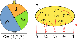
流形学习Manifold learningPCA识别数据中的三个主要成分。投影到前两个PCA分量导致沿歧管混合的颜色。流形学习(LLE和IsoMap)在投影数据时保留了局部结构,防止了颜色的混合。
statistics-lab™ 为您的留学生涯保驾护航 在代写流形学习Manifold learning方面已经树立了自己的口碑, 保证靠谱, 高质且原创的统计Statistics代写服务。我们的专家在代写流形学习Manifold learning代写方面经验极为丰富,各种代写流形学习Manifold learning相关的作业也就用不着说。
计算机代写|流形学习代写Manifold learning代考|Diffusion Maps
The basic idea of Diffusion MAPs (Nadler, Lafon, Coifman, and Kevrekidis, 2005; Coifman and Lafon, 2006) uses a Markov chain constructed over a graph of the data points, followed by an eigenanalysis of the probability transition matrix of the Markov chain. As with the other algorithms in this Section, there are three steps in this algorithm, with the first and second steps the same as for Laplacian eigenmaps. Although a nearest-neighbor search (Step 1) was not explicitly considered in the above papers on diffusion maps as a means of constructing the graph (Step 2), a nearest-neighbor search is included in software packages for computing diffusion maps. For an example in astronomy of a diffusion map incorporating a nearest-neighbor search, see Freeman, Newman, Lee, Richards, and Schafer (2009).
- Nearest-Neighbor Search. Fix an integer $K$ or an $\epsilon>0$. Define a $K$-neighborhood $N_i^K$ or an $\epsilon$-neighborhood $N_i^\epsilon$ of the point $\mathbf{x}_i$ as in Step 1 of Laplacian eigenmaps. In general, let $N_i$ denote the neighborhood of $\mathbf{x}_i$.
- Pairwise Adjacency Matrix. The $n$ data points $\left{\mathbf{x}i\right}$ in $\Re^r$ can be regarded as a graph $\mathcal{G}=\mathcal{G}(\mathcal{V}, \mathcal{E})$ with the data points playing the role of vertices $\mathcal{V}=\left{\mathbf{x}_1, \ldots, \mathbf{x}_n\right}$, and the set of edges $\mathcal{E}$ are the connection strengths (or weights), $w\left(\mathbf{x}_i, \mathbf{x}_j\right)$, between pairs of adjacent vertices, $$ w{i j}=w\left(\mathbf{x}i, \mathbf{x}_j\right)= \begin{cases}\exp \left{-\frac{\left|\mathbf{x}_i-\mathbf{x}_j\right|^2}{2 \sigma^2}\right}, & \text { if } \mathbf{x}_j \in N_i ; \ 0, & \text { otherwise. }\end{cases} $$ This is a Gaussian kernel with width $\sigma$; however, other kernels may be used. Kernels such as (1.52) ensure that the closer two points are to each other, the larger the value of $w$. For convenience in exposition, we will suppress the fact that the elements of most of the matrices depend upon the value of $\sigma$. Then, $\mathbf{W}=\left(w{i j}\right)$ is a pairwise adjacency matrix between the $n$ points. To make the matrix $\mathbf{W}$ even more sparse, values of its entries that are smaller than some given threshold (i.e., the points in question are far apart from each other) can be set to zero. The graph $\mathcal{G}$ with weight matrix $\mathbf{W}$ gives information on the local geometry of the data.
- Spectral embedding. Define $\mathbf{D}=\left(d_{i j}\right)$ to be a diagonal matrix formed from the matrix $\mathbf{W}$ by setting the diagonal elements, $d_{i i}=\sum_j w_{i j}$, to be the column sums of $\mathbf{W}$ and the off-diagonal elements to be zero. The $(n \times n)$ symmetric matrix $\mathbf{L}=\mathbf{D}-\mathbf{W}$ is the graph Laplacian for the graph $\mathcal{G}$. We are interested in the solutions of the generalized eigenequation, $\mathbf{L v}=\lambda \mathbf{D v}$, or, equivalently, of the matrix
$$
\mathbf{P}=\mathbf{D}^{-1 / 2} \mathbf{L} \mathbf{D}^{-1 / 2}=\mathbf{I}_n-\mathbf{D}^{-1 / 2} \mathbf{W} \mathbf{D}^{-1 / 2},
$$
which is the normalized graph Laplacian. The matrix $\mathbf{H}=e^{t \mathbf{P}}, t \geq 0$, is usually referred to as the heat kernel. By construction, $\mathbf{P}$ is a stochastic matrix with all row sums equal to one, and, thus, can be interpreted as defining a random walk on the graph $\mathcal{G}$.
计算机代写|流形学习代写Manifold learning代考|Hessian Eigenmaps
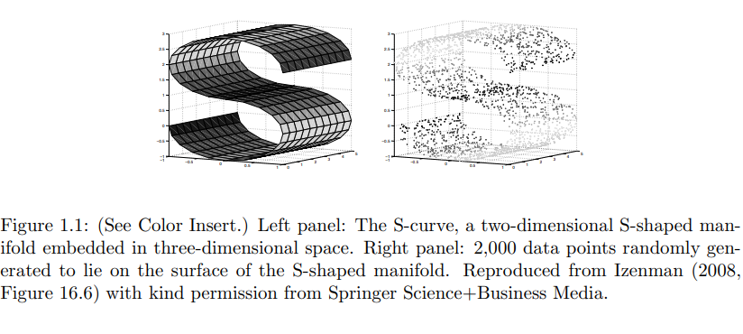
Recall that, in certain situations, the convexity assumption for IsomAP may be too restrictive. Instead, we may require that the manifold $\mathcal{M}$ be locally isometric to an open, connected subset of $\Re^t$. Popular examples include families of “articulated” images (i.e., translated or rotated images of the same object, possibly through time) that are found in a high-dimensional, digitized-image library (e.g., faces, pictures, handwritten numbers or letters). However, if the pixel elements of each 64-pixel-by-64-pixel digitized image are represented as a 4,096-dimensional vector in “pixel space,” it would be very difficult to show that the images really live on a low-dimensional manifold, especially if that image manifold is unknown.
We can model such images using a vector of smoothly varying articulation parameters $\boldsymbol{\theta} \in \Theta$. For example, digitized images of a person’s face that are varied by pose and illumination can be parameterized by two pose parameters (expression [happy, sad, sleepy, surprised, wink] and glasses-no glasses) and a lighting direction (centerlight, leftlight, rightlight, normal); similarly, handwritten “2”s appear to be parameterized essentially by two features, bottom loop and top arch (Tenenbaum, de Silva, and Langford, 2000; Roweis and Saul, 2000). To some extent, learning about an underlying image manifold depends upon whether the images are sufficiently scattered around the manifold and how good is the quality of digitization of each image?
Hessian Eigenmaps (Donoho and Grimes, 2003b) were proposed for recovering manifolds of high-dimensional libraries of articulated images where the convexity assumption is often violated. Let $\Theta \subset \Re^t$ be the parameter space and suppose that $\phi: \Theta \rightarrow \Re^r$, where $t<r$. Assume $\mathcal{M}=\phi(\Theta)$ is a smooth manifold of articulated images. The isometry and convexity requirements of IsOMAP are replaced by the following weaker requirements:
- Local Isometry: $\phi$ is a locally isometric embedding of $\Theta$ into $\Re^r$. For any point $\mathbf{x}^{\prime}$ in a sufficiently small neighborhood around each point $\mathrm{x}$ on the manifold $\mathcal{M}$, the geodesic distance equals the Euclidean distance between their corresponding parameter points $\boldsymbol{\theta}, \boldsymbol{\theta}^{\prime} \in \Theta ;$ that is,
$$
d^{\mathcal{M}}\left(\mathbf{x}, \mathbf{x}^{\prime}\right)=\left|\boldsymbol{\theta}-\boldsymbol{\theta}^{\prime}\right|_{\Theta},
$$
where $\mathbf{x}=\phi(\boldsymbol{\theta})$ and $\mathbf{x}^{\prime}=\phi\left(\boldsymbol{\theta}^{\prime}\right)$. - Connectedness: The parameter space $\Theta$ is an open, connected subset of $\Re^t$.
流形学习代写
计算机代写|流形学习代写Manifold learning代考|Diffusion Maps
扩散地图的基本思想(Nadler, Lafon, Coifman, and Kevrekidis, 2005;Coifman和Lafon, 2006)使用在数据点图上构造的马尔可夫链,然后对马尔可夫链的概率转移矩阵进行特征分析。与本节中的其他算法一样,该算法有三个步骤,第一步和第二步与拉普拉斯特征映射相同。尽管在上述关于扩散图的论文中,没有明确地将最近邻搜索(步骤1)作为构造图的一种方法(步骤2),但用于计算扩散图的软件包中包含了最近邻搜索。关于天文学中包含最近邻搜索的扩散图的例子,见Freeman, Newman, Lee, Richards, and Schafer(2009)。
最近邻搜索。修复整数$K$或$\epsilon>0$。定义点$\mathbf{x}_i$的$K$ -邻域$N_i^K$或$\epsilon$ -邻域$N_i^\epsilon$,如拉普拉斯特征映射的步骤1所示。通常,设$N_i$表示$\mathbf{x}_i$的邻域。
成对邻接矩阵。The $n$ 数据点 $\left{\mathbf{x}i\right}$ 在 $\Re^r$ 可以看作是一个图形吗 $\mathcal{G}=\mathcal{G}(\mathcal{V}, \mathcal{E})$ 用数据点扮演顶点的角色 $\mathcal{V}=\left{\mathbf{x}_1, \ldots, \mathbf{x}_n\right}$,以及边的集合 $\mathcal{E}$ 是连接强度(或权重), $w\left(\mathbf{x}_i, \mathbf{x}_j\right)$,相邻顶点对之间, $$ w{i j}=w\left(\mathbf{x}i, \mathbf{x}_j\right)= \begin{cases}\exp \left{-\frac{\left|\mathbf{x}_i-\mathbf{x}_j\right|^2}{2 \sigma^2}\right}, & \text { if } \mathbf{x}_j \in N_i ; \ 0, & \text { otherwise. }\end{cases} $$ 这是一个有宽度的高斯核 $\sigma$;但是,也可以使用其他内核。像(1.52)这样的核确保两个点越接近,的值就越大 $w$. 为了说明方便,我们将省略大多数矩阵的元素依赖于的值这一事实 $\sigma$. 然后, $\mathbf{W}=\left(w{i j}\right)$ 之间的成对邻接矩阵 $n$ 分。来制作矩阵 $\mathbf{W}$ 更稀疏的是,小于某个给定阈值(即,所讨论的点彼此相距很远)的条目值可以设置为零。图表 $\mathcal{G}$ 带权矩阵 $\mathbf{W}$ 给出有关数据局部几何形状的信息。
频谱嵌入。将$\mathbf{D}=\left(d_{i j}\right)$定义为由矩阵$\mathbf{W}$形成的对角矩阵,方法是将对角元素$d_{i i}=\sum_j w_{i j}$设置为$\mathbf{W}$的列和,并将非对角元素设置为零。$(n \times n)$对称矩阵$\mathbf{L}=\mathbf{D}-\mathbf{W}$是图$\mathcal{G}$的图拉普拉斯式。我们感兴趣的是广义特征方程$\mathbf{L v}=\lambda \mathbf{D v}$的解,或者,等价地,矩阵的解
$$
\mathbf{P}=\mathbf{D}^{-1 / 2} \mathbf{L} \mathbf{D}^{-1 / 2}=\mathbf{I}_n-\mathbf{D}^{-1 / 2} \mathbf{W} \mathbf{D}^{-1 / 2},
$$
也就是拉普拉斯归一化图。矩阵$\mathbf{H}=e^{t \mathbf{P}}, t \geq 0$,通常被称为热核。通过构造,$\mathbf{P}$是一个所有行和都等于1的随机矩阵,因此,可以解释为在图$\mathcal{G}$上定义了一个随机游走。
计算机代写|流形学习代写Manifold learning代考|Hessian Eigenmaps
回想一下,在某些情况下,IsomAP的凸性假设可能过于严格。相反,我们可能要求流形$\mathcal{M}$与$\Re^t$的一个开放的、连通的子集局部等距。流行的例子包括在高维数字化图像库(如面孔、图片、手写数字或字母)中发现的“关节”图像家族(即同一物体的翻译或旋转图像,可能是通过时间)。然而,如果每个64 × 64像素的数字化图像的像素元素在“像素空间”中被表示为一个4096维的向量,那么就很难表明这些图像确实存在于低维流形上,尤其是在该图像流形未知的情况下。
我们可以使用平滑变化的关节参数的向量$\boldsymbol{\theta} \in \Theta$对这样的图像进行建模。例如,根据姿势和光照变化的人脸数字化图像可以通过两个姿势参数(表情[高兴,悲伤,困倦,惊讶,眨眼]和戴眼镜-不戴眼镜)和光照方向(中心光,左光,右光,正常)来参数化;类似地,手写的“2”似乎主要由两个特征参数化,即底部环和顶部拱(Tenenbaum, de Silva, and Langford, 2000;Roweis and Saul, 2000)。在某种程度上,对底层图像流形的了解取决于图像是否充分分散在流形周围,以及每张图像的数字化质量有多好。
Hessian Eigenmaps (Donoho and Grimes, 2003b)被提出用于恢复经常违反凹凸性假设的高维铰接图像库的流形。设$\Theta \subset \Re^t$为参数空间,假设$\phi: \Theta \rightarrow \Re^r$,其中$t<r$。假设$\mathcal{M}=\phi(\Theta)$是一个平滑的铰接图像集合。IsOMAP的等距和凹凸性要求被以下较弱的要求所取代:
局部等距:$\phi$是在$\Re^r$中嵌入$\Theta$的局部等距。对于流形$\mathcal{M}$上每个点$\mathrm{x}$周围足够小的邻域内的任意点$\mathbf{x}^{\prime}$,测地线距离等于其对应参数点$\boldsymbol{\theta}, \boldsymbol{\theta}^{\prime} \in \Theta ;$之间的欧氏距离,即:
$$
d^{\mathcal{M}}\left(\mathbf{x}, \mathbf{x}^{\prime}\right)=\left|\boldsymbol{\theta}-\boldsymbol{\theta}^{\prime}\right|_{\Theta},
$$
其中$\mathbf{x}=\phi(\boldsymbol{\theta})$和$\mathbf{x}^{\prime}=\phi\left(\boldsymbol{\theta}^{\prime}\right)$。
连接性:参数空间$\Theta$是$\Re^t$的一个开放的、连接的子集。

统计代写请认准statistics-lab™. statistics-lab™为您的留学生涯保驾护航。
金融工程代写
金融工程是使用数学技术来解决金融问题。金融工程使用计算机科学、统计学、经济学和应用数学领域的工具和知识来解决当前的金融问题,以及设计新的和创新的金融产品。
非参数统计代写
非参数统计指的是一种统计方法,其中不假设数据来自于由少数参数决定的规定模型;这种模型的例子包括正态分布模型和线性回归模型。
广义线性模型代考
广义线性模型(GLM)归属统计学领域,是一种应用灵活的线性回归模型。该模型允许因变量的偏差分布有除了正态分布之外的其它分布。
术语 广义线性模型(GLM)通常是指给定连续和/或分类预测因素的连续响应变量的常规线性回归模型。它包括多元线性回归,以及方差分析和方差分析(仅含固定效应)。
有限元方法代写
有限元方法(FEM)是一种流行的方法,用于数值解决工程和数学建模中出现的微分方程。典型的问题领域包括结构分析、传热、流体流动、质量运输和电磁势等传统领域。
有限元是一种通用的数值方法,用于解决两个或三个空间变量的偏微分方程(即一些边界值问题)。为了解决一个问题,有限元将一个大系统细分为更小、更简单的部分,称为有限元。这是通过在空间维度上的特定空间离散化来实现的,它是通过构建对象的网格来实现的:用于求解的数值域,它有有限数量的点。边界值问题的有限元方法表述最终导致一个代数方程组。该方法在域上对未知函数进行逼近。[1] 然后将模拟这些有限元的简单方程组合成一个更大的方程系统,以模拟整个问题。然后,有限元通过变化微积分使相关的误差函数最小化来逼近一个解决方案。
tatistics-lab作为专业的留学生服务机构,多年来已为美国、英国、加拿大、澳洲等留学热门地的学生提供专业的学术服务,包括但不限于Essay代写,Assignment代写,Dissertation代写,Report代写,小组作业代写,Proposal代写,Paper代写,Presentation代写,计算机作业代写,论文修改和润色,网课代做,exam代考等等。写作范围涵盖高中,本科,研究生等海外留学全阶段,辐射金融,经济学,会计学,审计学,管理学等全球99%专业科目。写作团队既有专业英语母语作者,也有海外名校硕博留学生,每位写作老师都拥有过硬的语言能力,专业的学科背景和学术写作经验。我们承诺100%原创,100%专业,100%准时,100%满意。
随机分析代写
随机微积分是数学的一个分支,对随机过程进行操作。它允许为随机过程的积分定义一个关于随机过程的一致的积分理论。这个领域是由日本数学家伊藤清在第二次世界大战期间创建并开始的。
时间序列分析代写
随机过程,是依赖于参数的一组随机变量的全体,参数通常是时间。 随机变量是随机现象的数量表现,其时间序列是一组按照时间发生先后顺序进行排列的数据点序列。通常一组时间序列的时间间隔为一恒定值(如1秒,5分钟,12小时,7天,1年),因此时间序列可以作为离散时间数据进行分析处理。研究时间序列数据的意义在于现实中,往往需要研究某个事物其随时间发展变化的规律。这就需要通过研究该事物过去发展的历史记录,以得到其自身发展的规律。
回归分析代写
多元回归分析渐进(Multiple Regression Analysis Asymptotics)属于计量经济学领域,主要是一种数学上的统计分析方法,可以分析复杂情况下各影响因素的数学关系,在自然科学、社会和经济学等多个领域内应用广泛。
MATLAB代写
MATLAB 是一种用于技术计算的高性能语言。它将计算、可视化和编程集成在一个易于使用的环境中,其中问题和解决方案以熟悉的数学符号表示。典型用途包括:数学和计算算法开发建模、仿真和原型制作数据分析、探索和可视化科学和工程图形应用程序开发,包括图形用户界面构建MATLAB 是一个交互式系统,其基本数据元素是一个不需要维度的数组。这使您可以解决许多技术计算问题,尤其是那些具有矩阵和向量公式的问题,而只需用 C 或 Fortran 等标量非交互式语言编写程序所需的时间的一小部分。MATLAB 名称代表矩阵实验室。MATLAB 最初的编写目的是提供对由 LINPACK 和 EISPACK 项目开发的矩阵软件的轻松访问,这两个项目共同代表了矩阵计算软件的最新技术。MATLAB 经过多年的发展,得到了许多用户的投入。在大学环境中,它是数学、工程和科学入门和高级课程的标准教学工具。在工业领域,MATLAB 是高效研究、开发和分析的首选工具。MATLAB 具有一系列称为工具箱的特定于应用程序的解决方案。对于大多数 MATLAB 用户来说非常重要,工具箱允许您学习和应用专业技术。工具箱是 MATLAB 函数(M 文件)的综合集合,可扩展 MATLAB 环境以解决特定类别的问题。可用工具箱的领域包括信号处理、控制系统、神经网络、模糊逻辑、小波、仿真等。