标签: MATH2722

数学代写|数值分析代写numerical analysis代考|Inequality Constrained Optimization

如果你也在 怎样代写数值分析numerical analysis这个学科遇到相关的难题,请随时右上角联系我们的24/7代写客服。

数值分析是数学的一个分支,使用数字近似法解决连续问题。它涉及到设计能给出近似但精确的数字解决方案的方法,这在精确解决方案不可能或计算成本过高的情况下很有用。

statistics-lab™ 为您的留学生涯保驾护航 在代写数值分析numerical analysis方面已经树立了自己的口碑, 保证靠谱, 高质且原创的统计Statistics代写服务。我们的专家在代写数值分析numerical analysis代写方面经验极为丰富,各种代写数值分析numerical analysis相关的作业也就用不着说。

我们提供的数值分析numerical analysis及其相关学科的代写,服务范围广, 其中包括但不限于:

  • Statistical Inference 统计推断
  • Statistical Computing 统计计算
  • Advanced Probability Theory 高等概率论
  • Advanced Mathematical Statistics 高等数理统计学
  • (Generalized) Linear Models 广义线性模型
  • Statistical Machine Learning 统计机器学习
  • Longitudinal Data Analysis 纵向数据分析
  • Foundations of Data Science 数据科学基础

数学代写|数值分析代写numerical analysis代考|Inequality Constrained Optimization

Inequality constrained optimization is more complex, both in theory and practice. The theorem giving necessary conditions for inequality constrained optimization was only discovered in the middle of the twentieth century, while Lagrange used Lagrange multipliers in his Mécanique Analytique 151. The necessary conditions for inequality constrained optimization are called Kuhn-Tucker or Karush-Kuhn-Tucker conditions. The first journal publication with these conditions was a paper by Kuhn and Tucker in 149, although the essence of these conditions was contained in an unpublished Master’s thesis of Karush 139.

The work of Kuhn and Tucker was intended to build on the work of G. Dantzig and others [69] on linear programming:
$\min x c^T x \quad$ (8.6.7) subject to $$ A \boldsymbol{x} \geq \boldsymbol{b} $$ where ” $\boldsymbol{a} \geq \boldsymbol{b}$ ” is understood to mean ” $a_i \geq b_i$ for all $i$ “. It was Dantzig who created the simplex algorithm in 1946 [69], being the first general-purpose and efficient algorithm for solving linear programs (8.6.7, 8.6.8). The simplex method can be considered an example of an active set method as it tracks which of the inequalities $(A x)_i \geq b_i$ is actually an equality as it updates the candidate optimizer $\boldsymbol{x}$. Since then there has been a great deal of work on alternative methods, most notably interior point methods that typically minimize a sequence of penalized problems such as $$ c^T \boldsymbol{x}-\alpha \sum{i=1}^m \ln \left((A x)_i-b_i\right)
$$
where $\alpha>0$ is a parameter that is reduced to zero in the limit. The first published interior point method was due to Karmarkar 138. Another approach is the ellipsoidal method of Khachiyan 120, which at each step $k$ minimizes $\boldsymbol{c}^T \boldsymbol{x}$ over $\boldsymbol{x}$ lying inside an ellipsoid centered at $\boldsymbol{x}_k$ that is guaranteed to be inside the feasible set ${\boldsymbol{x} \mid A x \geq \boldsymbol{b}}$. Khachiyan’s ellipsoidal method built on previous ideas of N.Z. Shor but was the first guaranteed polynomial time algorithm for linear programming. Karmarkar’s algorithm also guaranteed polynomial time, but was much faster in practice than Khachiyan’s method and the first algorithm to have a better time than the simplex method on average.

数学代写|数值分析代写numerical analysis代考|Proving the Karush–Kuhn–Tucker Conditions

To prove the Karush-Kuhn-Tucker conditions we need a constraint qualification to ensure that
$$
T_{\Omega}(\boldsymbol{x})=\left{\boldsymbol{d} \mid \nabla g_i(\boldsymbol{x})^T \boldsymbol{d}=0 \text { for all } i \in \mathcal{E},\right.
$$
(8.6.9) $\nabla g_i(\boldsymbol{x})^T \boldsymbol{d} \geq 0$ for all $i \in \mathcal{I}$ where $\left.g_i(\boldsymbol{x})=0\right}=C_{\Omega}(\boldsymbol{x})$.
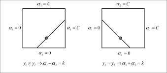
A constraint $g_i(\boldsymbol{x}) \geq 0$ is called active at $\boldsymbol{x}$ if $g_i(\boldsymbol{x})=0$ and inactive at $\boldsymbol{x}$ if $g_i(\boldsymbol{x})>0$. Inactive inequality constraints at $x$ do not affect the shape of the feasible set $\Omega$ near to $\boldsymbol{x}$. We designate the set of active constraints by
$$
\mathcal{A}(\boldsymbol{x})=\left{i \mid i \in \mathcal{E} \cup \mathcal{I} \text { and } g_i(\boldsymbol{x})=0\right} .
$$
The equivalence (8.6.9) holds under a number of constraint qualifications, the most used of which is the Linear Independence Constraint Qualification (LICQ) for inequality constrained optimization:
(8.6.11) $\quad\left{\nabla g_i(\boldsymbol{x}) \mid i \in \mathcal{A}(\boldsymbol{x})\right}$ is a linearly independent set.
Weaker constraint qualifications that guarantee (8.6.9) include the MangasarianFromowitz constraint qualification (MFCQ):
$\left{\nabla g_i(\boldsymbol{x}) \mid i \in \mathcal{E}\right}$ is a linearly independent set, and there is $\boldsymbol{d}$ where $\nabla g_i(\boldsymbol{x})^T \boldsymbol{d}=0$ for all $i \in \mathcal{E}$, and
$$
\nabla g_i(\boldsymbol{x})^T \boldsymbol{d}>0 \text { for all } i \in \mathcal{I} \cap \mathcal{A}(\boldsymbol{x}) .
$$
With a suitable constraint qualification, we can prove the existence of Lagrange multipliers satisfying the Karush-Kuhn-Tucker conditions.

数值分析代考

数学代写|数值分析代写numerical analysis代考|Inequality Constrained Optimization

不等式约束优化在理论上和实践上都更为复杂。给出不等式约束优化必要条件的定理直到二十世纪中叶 才被发现,而拉格朗日在他的《力学分析》151中使用了拉格朗日乘数。不等式约束优化的必要条件称为 Kuhn-Tucker 或 Karush-Kuhn-Tucker 条件。第一篇具有这些条件的期刊出版物是 Kuhn 和 Tucker 在 149发表的一篇论文,尽管这些条件的本质包含在 Karush 139末发表的硕士论文中。
Kuhn 和 Tucker 的工作旨在建立在 G. Dantzig 和其他人 [69] 关于线性规划的工作之上: $\min x c^T x \quad(8.6 .7)$ 受制于
$$
A \boldsymbol{x} \geq \boldsymbol{b}
$$
于求解线性规划的通用且高效的算法 (8.6.7,8.6.8)。单纯形法可以被认为是活动集方法的一个例子,因为 它跟踪哪些不等式 $(A x)_i \geq b_i$ 实际上是一个等式,因为它更新了候选优化器 $\boldsymbol{x}$. 从那时起,就替代方法 进行了大量工作,最著名的是内点方法,它通常最大限度地减少一系列惩恩问题,例如
$$
c^T \boldsymbol{x}-\alpha \sum i=1^m \ln \left((A x)_i-b_i\right)
$$
在哪里 $\alpha>0$ 是一个参数,在极限中减少到零。第一个发布的内点方法是由于 Karmarkar 138。另一种 方法是 Khachiyan 120的椭圆方法,它在每一步 $k$ 最小化 $\boldsymbol{c}^T \boldsymbol{x}$ 超过 $\boldsymbol{x}$ 位于以 为中心的椭圆体内 $\boldsymbol{x}_k$ 保证在 可行集内 $\boldsymbol{x} \mid A \boldsymbol{x} \geq \boldsymbol{b}$. Khachiyan 的椭圆体方法建立在 NZ Shor 之前的思想之上,但却是线性规划的第 一个保证多项式时间算法。Karmarkar 的算法也保证多项式时间,但在实践中比 Khachiyan 的方法快得 多,并且是第一个平均时间比单纯形法有更好时间的算法。

数学代写|数值分析代写numerical analysis代考|Proving the Karush–Kuhn–Tucker Conditions

为了证明 Karush-Kuhn-Tucker 条件,我们需要一个约束条件来确保
$$
T_{\Omega}(\boldsymbol{x})=\left{\boldsymbol{d} \mid \nabla g_i(\boldsymbol{x})^T \boldsymbol{d}=0 \text { for all } i \在 \mathcal{E} 中,\对。
$$
(8.6.9) $\nabla g_i(\boldsymbol{x})^T \boldsymbol{d} \geq 0$ 对于所有 $i \in \mathcal{I}$ 其中 $\left.g_i(\boldsymbol{x })=0\right}=C_{\Omega}(\boldsymbol{x})$。
如果 $g_i(\boldsymbol{x})=0$,约束 $g_i(\boldsymbol{x}) \geq 0$ 被称为在 $\boldsymbol{x}$ 处于活动状态,如果 $\boldsymbol{x}$ 处于非活动状态,则$g_i(\boldsymbol{x})>0$。 $x$ 处的非活动不等式约束不会影响 $\boldsymbol{x}$ 附近可行集 $\Omega$ 的形状。我们通过以下方式指定一组活动约束
$$
\mathcal{A}(\boldsymbol{x})=\left{i \mid i \in \mathcal{E} \cup \mathcal{I} \text { and } g_i(\boldsymbol{x})=0\正确的} 。
$$
等价 (8.6.9) 在许多约束条件下成立,其中最常用的是用于不等式约束优化的线性独立约束条件 (LICQ):
(8.6.11) $\quad\left{\nabla g_i(\boldsymbol{x}) \mid i \in \mathcal{A}(\boldsymbol{x})\right}$ 是线性独立集。
保证 (8.6.9) 的较弱约束条件包括 MangasarianFromowitz 约束条件 (MFCQ):
$\left{\nabla g_i(\boldsymbol{x}) \mid i \in \mathcal{E}\right}$ 是线性独立集,有 $\boldsymbol{d}$ 其中 $\nabla g_i( \boldsymbol{x})^T \boldsymbol{d}=0$ 对于所有 $i \in \mathcal{E}$,并且
$$
\nabla g_i(\boldsymbol{x})^T \boldsymbol{d}>0 \text { for all } i \in \mathcal{I} \cap \mathcal{A}(\boldsymbol{x}) 。
$$
通过适当的约束条件,我们可以证明满足 Karush-Kuhn-Tucker 条件的拉格朗日乘子的存在性
数学代写|数值分析代写numerical analysis代考 请认准statistics-lab™

统计代写请认准statistics-lab™. statistics-lab™为您的留学生涯保驾护航。

金融工程代写

金融工程是使用数学技术来解决金融问题。金融工程使用计算机科学、统计学、经济学和应用数学领域的工具和知识来解决当前的金融问题,以及设计新的和创新的金融产品。

非参数统计代写

非参数统计指的是一种统计方法,其中不假设数据来自于由少数参数决定的规定模型;这种模型的例子包括正态分布模型和线性回归模型。

广义线性模型代考

广义线性模型(GLM)归属统计学领域,是一种应用灵活的线性回归模型。该模型允许因变量的偏差分布有除了正态分布之外的其它分布。

术语 广义线性模型(GLM)通常是指给定连续和/或分类预测因素的连续响应变量的常规线性回归模型。它包括多元线性回归,以及方差分析和方差分析(仅含固定效应)。

有限元方法代写

有限元方法(FEM)是一种流行的方法,用于数值解决工程和数学建模中出现的微分方程。典型的问题领域包括结构分析、传热、流体流动、质量运输和电磁势等传统领域。

有限元是一种通用的数值方法,用于解决两个或三个空间变量的偏微分方程(即一些边界值问题)。为了解决一个问题,有限元将一个大系统细分为更小、更简单的部分,称为有限元。这是通过在空间维度上的特定空间离散化来实现的,它是通过构建对象的网格来实现的:用于求解的数值域,它有有限数量的点。边界值问题的有限元方法表述最终导致一个代数方程组。该方法在域上对未知函数进行逼近。[1] 然后将模拟这些有限元的简单方程组合成一个更大的方程系统,以模拟整个问题。然后,有限元通过变化微积分使相关的误差函数最小化来逼近一个解决方案。

tatistics-lab作为专业的留学生服务机构,多年来已为美国、英国、加拿大、澳洲等留学热门地的学生提供专业的学术服务,包括但不限于Essay代写,Assignment代写,Dissertation代写,Report代写,小组作业代写,Proposal代写,Paper代写,Presentation代写,计算机作业代写,论文修改和润色,网课代做,exam代考等等。写作范围涵盖高中,本科,研究生等海外留学全阶段,辐射金融,经济学,会计学,审计学,管理学等全球99%专业科目。写作团队既有专业英语母语作者,也有海外名校硕博留学生,每位写作老师都拥有过硬的语言能力,专业的学科背景和学术写作经验。我们承诺100%原创,100%专业,100%准时,100%满意。

随机分析代写


随机微积分是数学的一个分支,对随机过程进行操作。它允许为随机过程的积分定义一个关于随机过程的一致的积分理论。这个领域是由日本数学家伊藤清在第二次世界大战期间创建并开始的。

时间序列分析代写

随机过程,是依赖于参数的一组随机变量的全体,参数通常是时间。 随机变量是随机现象的数量表现,其时间序列是一组按照时间发生先后顺序进行排列的数据点序列。通常一组时间序列的时间间隔为一恒定值(如1秒,5分钟,12小时,7天,1年),因此时间序列可以作为离散时间数据进行分析处理。研究时间序列数据的意义在于现实中,往往需要研究某个事物其随时间发展变化的规律。这就需要通过研究该事物过去发展的历史记录,以得到其自身发展的规律。

回归分析代写

多元回归分析渐进(Multiple Regression Analysis Asymptotics)属于计量经济学领域,主要是一种数学上的统计分析方法,可以分析复杂情况下各影响因素的数学关系,在自然科学、社会和经济学等多个领域内应用广泛。

MATLAB代写

MATLAB 是一种用于技术计算的高性能语言。它将计算、可视化和编程集成在一个易于使用的环境中,其中问题和解决方案以熟悉的数学符号表示。典型用途包括:数学和计算算法开发建模、仿真和原型制作数据分析、探索和可视化科学和工程图形应用程序开发,包括图形用户界面构建MATLAB 是一个交互式系统,其基本数据元素是一个不需要维度的数组。这使您可以解决许多技术计算问题,尤其是那些具有矩阵和向量公式的问题,而只需用 C 或 Fortran 等标量非交互式语言编写程序所需的时间的一小部分。MATLAB 名称代表矩阵实验室。MATLAB 最初的编写目的是提供对由 LINPACK 和 EISPACK 项目开发的矩阵软件的轻松访问,这两个项目共同代表了矩阵计算软件的最新技术。MATLAB 经过多年的发展,得到了许多用户的投入。在大学环境中,它是数学、工程和科学入门和高级课程的标准教学工具。在工业领域,MATLAB 是高效研究、开发和分析的首选工具。MATLAB 具有一系列称为工具箱的特定于应用程序的解决方案。对于大多数 MATLAB 用户来说非常重要,工具箱允许您学习应用专业技术。工具箱是 MATLAB 函数(M 文件)的综合集合,可扩展 MATLAB 环境以解决特定类别的问题。可用工具箱的领域包括信号处理、控制系统、神经网络、模糊逻辑、小波、仿真等。

R语言代写问卷设计与分析代写
PYTHON代写回归分析与线性模型代写
MATLAB代写方差分析与试验设计代写
STATA代写机器学习/统计学习代写
SPSS代写计量经济学代写
EVIEWS代写时间序列分析代写
EXCEL代写深度学习代写
SQL代写各种数据建模与可视化代写

数学代写|数值分析代写numerical analysis代考|Constrained Optimization

如果你也在 怎样代写数值分析numerical analysis这个学科遇到相关的难题,请随时右上角联系我们的24/7代写客服。

数值分析是数学的一个分支,使用数字近似法解决连续问题。它涉及到设计能给出近似但精确的数字解决方案的方法,这在精确解决方案不可能或计算成本过高的情况下很有用。

statistics-lab™ 为您的留学生涯保驾护航 在代写数值分析numerical analysis方面已经树立了自己的口碑, 保证靠谱, 高质且原创的统计Statistics代写服务。我们的专家在代写数值分析numerical analysis代写方面经验极为丰富,各种代写数值分析numerical analysis相关的作业也就用不着说。

我们提供的数值分析numerical analysis及其相关学科的代写,服务范围广, 其中包括但不限于:

  • Statistical Inference 统计推断
  • Statistical Computing 统计计算
  • Advanced Probability Theory 高等概率论
  • Advanced Mathematical Statistics 高等数理统计学
  • (Generalized) Linear Models 广义线性模型
  • Statistical Machine Learning 统计机器学习
  • Longitudinal Data Analysis 纵向数据分析
  • Foundations of Data Science 数据科学基础

数学代写|数值分析代写numerical analysis代考|Constrained Optimization

Constrained optimization can be represented most abstractly in terms of a feasible set, often denoted $\Omega \subseteq \mathbb{R}^n$ :
(8.6.1) $\min _x f(x) \quad$ subject to $x \in \Omega$
Solutions exist if $f$ is continuous and either $\Omega$ is a compact (closed and bounded) subset of $\mathbb{R}^n$, or if $\Omega$ is closed and $f$ is coercive. Usually $\Omega$ is represented by equations and inequalities:
(8.6.2) $\Omega=\left{\boldsymbol{x} \in \mathbb{R}^n \mid g_i(\boldsymbol{x})=0\right.$ for $i \in \mathcal{E}$, and $g_i(\boldsymbol{x}) \geq 0$ for $\left.i \in \mathcal{I}\right}$.
If $\mathcal{I}$ is empty but $\mathcal{E}$ is not empty, then we say (8.6.1) is an equality constrained optimization problem. If $\mathcal{I}$ is non-empty, we say (8.6.1) is an inequality constrained optimization problem.

For a general constrained optimization problem, first-order conditions can be given in terms of the tangent cone
$(8.6 .3)$
$$
T_{\Omega}(\boldsymbol{x})=\left{\lim _{k \rightarrow \infty} \frac{\boldsymbol{x}_k-\boldsymbol{x}}{t_k} \mid \boldsymbol{x}_k \in \Omega, \boldsymbol{x}_k \rightarrow \boldsymbol{x} \text { as } k \rightarrow \infty \text {, and } t_k \downarrow 0 \text { as } k \rightarrow \infty\right}
$$

Lemma 8.19 If $\boldsymbol{x}=x^$ minimizes $f(x)$ over $\boldsymbol{x} \in \Omega$ and $f$ is differentiable at $\boldsymbol{x}^$, then
(8.6.4) $\nabla f\left(x^\right)^T d \geq 0 \quad$ for all $d \in T_{\Omega}\left(x^\right)$.
Proof Suppose $x=x^* \in \Omega$ minimizes $f(x)$ over $x \in \Omega$ and $f$ is differentiable. Then for any $\boldsymbol{d} \in T_{\Omega}\left(\boldsymbol{x}^\right)$, there is a sequence $\boldsymbol{x}k \rightarrow \boldsymbol{x}^$ as $k \rightarrow \infty$ with $\boldsymbol{x}_k \in \Omega$ where $\boldsymbol{d}_k:=\left(\boldsymbol{x}_k-\boldsymbol{x}^\right) / t_k \rightarrow \boldsymbol{d}$ as $k \rightarrow \infty$. Since $f\left(\boldsymbol{x}^\right) \leq f\left(\boldsymbol{x}_k\right)=f\left(\boldsymbol{x}^+t_k \boldsymbol{d}_k\right)$, $$ 0 \leq \lim {k \rightarrow \infty} \frac{f\left(x^+t_k \boldsymbol{d}k\right)-f\left(x^\right)}{t_k}=\nabla f\left(x^\right)^T \lim {k \rightarrow \infty} \boldsymbol{d}k=\nabla f\left(x^\right)^T \boldsymbol{d} . $$ This holds for any $d \in T{\Omega}\left(x^\right)$ showing (8.6.4), as we wanted.
Constraint qualifications relate the tangent cone $T_{\Omega}(\boldsymbol{x})$ to the linearizations of the constraint functions:
$$
\begin{aligned}
& C_{\Omega}(\boldsymbol{x})=\left{\boldsymbol{d} \in \mathbb{R}^n \mid \nabla g_i(\boldsymbol{x})^T \boldsymbol{d}=0 \text { for all } i \in \mathcal{E},\right. \
& \left.\quad \nabla g_i(\boldsymbol{x})^T \boldsymbol{d} \geq 0 \text { for all } i \in \mathcal{I} \text { where } g_i(\boldsymbol{x})=0\right} .
\end{aligned}
$$
For equality constrained optimization $(\mathcal{I}=\emptyset)$, the LICQ (8.1.2) implies that $T_{\Omega}(\boldsymbol{x})=C_{\Omega}(\boldsymbol{x})$ as noted in Section 8.1.3.

数学代写|数值分析代写numerical analysis代考|Equality Constrained Optimization

The theory of Section 8.1.3 for Lagrange multipliers and equality constrained optimization (8.1.5) can be immediately turned into a numerical method. To solve
$$
\begin{aligned}
& \mathbf{0}=\nabla f(\boldsymbol{x})-\sum_{i \in \mathcal{E}} \lambda_i \nabla g(\boldsymbol{x}) \
& 0=g_i(\boldsymbol{x}), \quad i \in \mathcal{E}
\end{aligned}
$$
for $(\boldsymbol{x}, \boldsymbol{\lambda})$ with $\boldsymbol{\lambda}=\left[\lambda_i \mid i \in \mathcal{E}\right]$ we can apply, for example, Newton’s method. For unconstrained optimization, we can then perform a line search to ensure that the step improves the solution estimate. The issue in constrained optimization is that $f(\boldsymbol{x})$ alone is no longer suitable for measuring improvements. Constrained optimization problems have two objectives: staying on the feasible set, and minimizing $f(\boldsymbol{x})$. It may be necessary to increase $f(\boldsymbol{x})$ in order to return to the feasible set. Solving the Newton equations for $(8.6 .5,8.6 .6)$ gives a direction $\boldsymbol{d}$. Because of the curvature of the feasible set $\Omega$ for general functions $g_i$, moving in the direction $\boldsymbol{d}$ even if $\boldsymbol{x}$ is feasible may take the point $\boldsymbol{x}+s \boldsymbol{d}$ off the feasible set. This can be offset by having a second order correction step to move back toward the feasible set. This second order correction uses a least squares version of Newton’s method to solve $g(\boldsymbol{x})=\mathbf{0}$.

Since this is an under-determined system for $|\mathcal{E}|<n$, we find the solution $\delta \boldsymbol{x}$ for $\nabla g_i(\boldsymbol{x})^T \delta \boldsymbol{x}=-g_i(\boldsymbol{x}), i \in \mathcal{E}$, that minimizes $|\delta \boldsymbol{x}|_2$, which can be done using the QR factorization of $\left[\nabla g_i(\boldsymbol{x}) \mid i \in \mathcal{E}\right]$.

For line search algorithms, we can use a merit function to determine the quality of the result of the step. Often, merit functions of the form $\boldsymbol{x} \mapsto f(\boldsymbol{x})+\alpha \sum_{i \in \mathcal{E}}\left|g_i(\boldsymbol{x})\right|$ are used where $\alpha>\max _{i \in \mathcal{E}}\left|\lambda_i\right|$. A basic method for solving equality constrained optimization problems is shown in Algorithm 82.

If the second-order correction is skipped, then the Newton method may fail to give rapid convergence, as was noted by N. Maratos in his PhD thesis [170].

数值分析代考

数学代写|数值分析代写numerical analysis代考|Constrained Optimization

约束优化可以用可行集最抽象地表示,通常表示为 $\Omega \subseteq \mathbb{R}^n$ :
(8.6.1) $\min x f(x) \quad$ 受制于 $x \in \Omega$ 如果存在解决方案 $f$ 是连续的,并且 $\Omega$ 是一个紧凑的(封闭和有界的) 子集 $\mathbb{R}^n$ ,或者如果 $\Omega$ 关闭并且 $f$ 是强制性的。通常 $\Omega$ 由方程式和不等式表示: $(8.6 .2)$ \Omega $=\backslash$ \eft $\left{\backslash\right.$ boldsymbol ${x} \backslash$ in $\backslash m a t h b b{R} \wedge n \backslash m i d g _i(\wedge b o l d s y m b o l{x})=0 \backslash r i g h t . \$$ 对于 $\$ i \backslash$ in $\backslash m a t h c a \mid{E} \$$ 和 如果 $\mathcal{I}$ 是空的但是 $\mathcal{E}$ 不为空,那么我们说 (8.6.1) 是一个等式约束优化问题。如果 $\mathcal{I}$ 是非空的,我们说 (8.6.1) 是一个不等式约束优化问题。 对于一般的约束优化问题,可以根据切锥给出一阶条件 $T{_} _{\backslash \text { omega }}($ boldsymbol ${x})=\backslash$ left ${\backslash$ lim_{k $\backslash$ rightarrow $\backslash$ infty $} \backslash f r a c\left{\backslash b o l d s y m b o l{x} _k-l b o l d s y m b o l{x}\right}\left{t _k\right} \backslash m i$
证明假设 $x=x^* \in \Omega$ 最小化 $f(x)$ 超过 $x \in \Omega$ 和 $f$ 是可微分的。然后对于任何
Iboldsymbol{x}k \rightarrow \boldsymbol{{x}^ 作为 $k \rightarrow \infty$ 和 $x_k \in \Omega$ 在哪里
$k \rightarrow \infty$. 自从
这适用于任何 $d \backslash$ in $T{\backslash O m e g a} \backslash$ left( $\left.x^{\wedge} \backslash r i g h t\right)$ 显示 (8.6.4),如我们所愿。
约束条件与切锥相关 $T_{\Omega}(x)$ 约束函数的线性化:
\begin{aligned } } \text { \& C_{१Omega } } ( \backslash b o l d s y m b o l { x } ) = \backslash \text { left } { \text { boldsymbol{d } } \text { in } \backslash m a t h b b { R } ^ { \wedge } n \backslash m i d \backslash \text { nabla g_i(\boldsy }
对于等式约束优化 $(\mathcal{I}=\emptyset) ,$ LICQ (8.1.2) 意味着 $T_{\Omega}(\boldsymbol{x})=C_{\Omega}(\boldsymbol{x})$ 如第 8.1.3 节所述。

数学代写|数值分析代写numerical analysis代考|Equality Constrained Optimization

8.1.3 节关于拉格朗日乘数和等式约束优化 (8.1.5) 的理论可以立即转化为数值方法。解决
$$
\mathbf{0}=\nabla f(\boldsymbol{x})-\sum_{i \in \mathcal{E}} \lambda_i \nabla g(\boldsymbol{x}) \quad 0=g_i(\boldsymbol{x}), \quad i \in \mathcal{E}
$$
为了 $(\boldsymbol{x}, \boldsymbol{\lambda})$ 和 $\boldsymbol{\lambda}=\left[\lambda_i \mid i \in \mathcal{E}\right]$ 例如,我们可以应用牛顿法。对于无约束优化,我们可以执行线搜索以 确保该步骙改进解估计。约束优化的问题是 $f(\boldsymbol{x})$ 单独不再适合衡量改进。约束优化问题有两个目标:保 持在可行集上,并最小化 $f(\boldsymbol{x})$. 可能需要增加 $f(\boldsymbol{x})$ 为了回到可行集。求解牛顿方程 $(8.6 .5,8.6 .6)$ 给出 方向 $\boldsymbol{d}$. 由于可行集的曲率 $\Omega$ 用于一般功能 $g_i$, 朝着这个方向移动 $\boldsymbol{d}$ 即使 $\boldsymbol{x}$ 可行可以拿点 $\boldsymbol{x}+s \boldsymbol{d}$ 脱离可行 集。这可以通过使用二阶校正步骙返回可行集来抵消。此二阶校正使用牛顿法的最小二乘法来求解 $g(\boldsymbol{x})=\mathbf{0}$
因为这是一个欠定的系统 $|\mathcal{E}|2$ ,这可以使用 QR 因式分解来完成 $\left[\nabla g_i(\boldsymbol{x}) \mid i \in \mathcal{E}\right]$. 对于线搜索算法,我们可以使用评价函数来确定步骤结果的质量。通常,形式的评价函数 $\boldsymbol{x} \mapsto f(\boldsymbol{x})+\alpha \sum{i \in \mathcal{E}}\left|g_i(\boldsymbol{x})\right|$ 在哪里使用 $\alpha>\max _{i \in \mathcal{E}}\left|\lambda_i\right|$. 算法 82 显示了解决等式约束优化问题的 基本方法。
如果跳过二阶校正,那么牛顿法可能无法提供快速收敛,正如 N. Maratos 在他的博士论文 [170] 中指出 的那样。

数学代写|数值分析代写numerical analysis代考 请认准statistics-lab™

统计代写请认准statistics-lab™. statistics-lab™为您的留学生涯保驾护航。

金融工程代写

金融工程是使用数学技术来解决金融问题。金融工程使用计算机科学、统计学、经济学和应用数学领域的工具和知识来解决当前的金融问题,以及设计新的和创新的金融产品。

非参数统计代写

非参数统计指的是一种统计方法,其中不假设数据来自于由少数参数决定的规定模型;这种模型的例子包括正态分布模型和线性回归模型。

广义线性模型代考

广义线性模型(GLM)归属统计学领域,是一种应用灵活的线性回归模型。该模型允许因变量的偏差分布有除了正态分布之外的其它分布。

术语 广义线性模型(GLM)通常是指给定连续和/或分类预测因素的连续响应变量的常规线性回归模型。它包括多元线性回归,以及方差分析和方差分析(仅含固定效应)。

有限元方法代写

有限元方法(FEM)是一种流行的方法,用于数值解决工程和数学建模中出现的微分方程。典型的问题领域包括结构分析、传热、流体流动、质量运输和电磁势等传统领域。

有限元是一种通用的数值方法,用于解决两个或三个空间变量的偏微分方程(即一些边界值问题)。为了解决一个问题,有限元将一个大系统细分为更小、更简单的部分,称为有限元。这是通过在空间维度上的特定空间离散化来实现的,它是通过构建对象的网格来实现的:用于求解的数值域,它有有限数量的点。边界值问题的有限元方法表述最终导致一个代数方程组。该方法在域上对未知函数进行逼近。[1] 然后将模拟这些有限元的简单方程组合成一个更大的方程系统,以模拟整个问题。然后,有限元通过变化微积分使相关的误差函数最小化来逼近一个解决方案。

tatistics-lab作为专业的留学生服务机构,多年来已为美国、英国、加拿大、澳洲等留学热门地的学生提供专业的学术服务,包括但不限于Essay代写,Assignment代写,Dissertation代写,Report代写,小组作业代写,Proposal代写,Paper代写,Presentation代写,计算机作业代写,论文修改和润色,网课代做,exam代考等等。写作范围涵盖高中,本科,研究生等海外留学全阶段,辐射金融,经济学,会计学,审计学,管理学等全球99%专业科目。写作团队既有专业英语母语作者,也有海外名校硕博留学生,每位写作老师都拥有过硬的语言能力,专业的学科背景和学术写作经验。我们承诺100%原创,100%专业,100%准时,100%满意。

随机分析代写


随机微积分是数学的一个分支,对随机过程进行操作。它允许为随机过程的积分定义一个关于随机过程的一致的积分理论。这个领域是由日本数学家伊藤清在第二次世界大战期间创建并开始的。

时间序列分析代写

随机过程,是依赖于参数的一组随机变量的全体,参数通常是时间。 随机变量是随机现象的数量表现,其时间序列是一组按照时间发生先后顺序进行排列的数据点序列。通常一组时间序列的时间间隔为一恒定值(如1秒,5分钟,12小时,7天,1年),因此时间序列可以作为离散时间数据进行分析处理。研究时间序列数据的意义在于现实中,往往需要研究某个事物其随时间发展变化的规律。这就需要通过研究该事物过去发展的历史记录,以得到其自身发展的规律。

回归分析代写

多元回归分析渐进(Multiple Regression Analysis Asymptotics)属于计量经济学领域,主要是一种数学上的统计分析方法,可以分析复杂情况下各影响因素的数学关系,在自然科学、社会和经济学等多个领域内应用广泛。

MATLAB代写

MATLAB 是一种用于技术计算的高性能语言。它将计算、可视化和编程集成在一个易于使用的环境中,其中问题和解决方案以熟悉的数学符号表示。典型用途包括:数学和计算算法开发建模、仿真和原型制作数据分析、探索和可视化科学和工程图形应用程序开发,包括图形用户界面构建MATLAB 是一个交互式系统,其基本数据元素是一个不需要维度的数组。这使您可以解决许多技术计算问题,尤其是那些具有矩阵和向量公式的问题,而只需用 C 或 Fortran 等标量非交互式语言编写程序所需的时间的一小部分。MATLAB 名称代表矩阵实验室。MATLAB 最初的编写目的是提供对由 LINPACK 和 EISPACK 项目开发的矩阵软件的轻松访问,这两个项目共同代表了矩阵计算软件的最新技术。MATLAB 经过多年的发展,得到了许多用户的投入。在大学环境中,它是数学、工程和科学入门和高级课程的标准教学工具。在工业领域,MATLAB 是高效研究、开发和分析的首选工具。MATLAB 具有一系列称为工具箱的特定于应用程序的解决方案。对于大多数 MATLAB 用户来说非常重要,工具箱允许您学习应用专业技术。工具箱是 MATLAB 函数(M 文件)的综合集合,可扩展 MATLAB 环境以解决特定类别的问题。可用工具箱的领域包括信号处理、控制系统、神经网络、模糊逻辑、小波、仿真等。

R语言代写问卷设计与分析代写
PYTHON代写回归分析与线性模型代写
MATLAB代写方差分析与试验设计代写
STATA代写机器学习/统计学习代写
SPSS代写计量经济学代写
EVIEWS代写时间序列分析代写
EXCEL代写深度学习代写
SQL代写各种数据建模与可视化代写

数学代写|数值分析代写numerical analysis代考|Convex and Non-convex

如果你也在 怎样代写数值分析numerical analysis这个学科遇到相关的难题,请随时右上角联系我们的24/7代写客服。

数值分析是数学的一个分支,使用数字近似法解决连续问题。它涉及到设计能给出近似但精确的数字解决方案的方法,这在精确解决方案不可能或计算成本过高的情况下很有用。

statistics-lab™ 为您的留学生涯保驾护航 在代写数值分析numerical analysis方面已经树立了自己的口碑, 保证靠谱, 高质且原创的统计Statistics代写服务。我们的专家在代写数值分析numerical analysis代写方面经验极为丰富,各种代写数值分析numerical analysis相关的作业也就用不着说。

我们提供的数值分析numerical analysis及其相关学科的代写,服务范围广, 其中包括但不限于:

  • Statistical Inference 统计推断
  • Statistical Computing 统计计算
  • Advanced Probability Theory 高等概率论
  • Advanced Mathematical Statistics 高等数理统计学
  • (Generalized) Linear Models 广义线性模型
  • Statistical Machine Learning 统计机器学习
  • Longitudinal Data Analysis 纵向数据分析
  • Foundations of Data Science 数据科学基础

数学代写|数值分析代写numerical analysis代考|Convex Functions

A function $\varphi: \mathbb{R}^n \rightarrow \mathbb{R}$ is convex if for any $\boldsymbol{x}, \boldsymbol{y} \in \mathbb{R}^n$ and $0 \leq \theta \leq 1$, then $\varphi(\theta \boldsymbol{x}+(1-\theta) \boldsymbol{y}) \leq \theta \varphi(\boldsymbol{x})+(1-\theta) \varphi(\boldsymbol{y})$.
Convex functions are very important in optimization theory. Convex functions can be smooth or not smooth. But they cannot be discontinuous unless we allow “+ + ” as a value they can have. We say that $\varphi$ is strictly convex if for any $\boldsymbol{x} \neq \boldsymbol{y} \in \mathbb{R}^n$ and $0<\theta<1$ $\varphi(\theta \boldsymbol{x}+(1-\theta) \boldsymbol{y})<\theta \varphi(\boldsymbol{x})+(1-\theta) \varphi(\boldsymbol{y})$ If $f$ is smooth there are equivalent ways of telling if a function is convex. Theorem 8.9 If $f: \mathbb{R}^n \rightarrow \mathbb{R}$ has continuous first derivatives, then $f$ is convex if and only if (8.2.3) $f(\boldsymbol{y}) \geq f(\boldsymbol{x})+\nabla f(\boldsymbol{x})^T(\boldsymbol{y}-\boldsymbol{x}) \quad$ for all $\boldsymbol{x}, \boldsymbol{y} \in \mathbb{R}^n$. Proof Suppose that $f$ is convex. Then for any $\boldsymbol{x}, \boldsymbol{y} \in \mathbb{R}^n$ and $0 \leq \theta \leq 1$, $$ f(\theta x+(1-\theta) y) \leq \theta f(x)+(1-\theta) f(y) $$ Put $\rho=1-\theta$, which is also between zero and one: $$ f((1-\rho) \boldsymbol{x}+\rho \boldsymbol{y}) \leq(1-\rho) f(\boldsymbol{x})+\rho f(\boldsymbol{y}) $$ Subtracting $f(\boldsymbol{x})$ from both sides and dividing by $\rho>0$ :
$$
\frac{f(\boldsymbol{x}+\rho(\boldsymbol{y}-\boldsymbol{x}))-f(\boldsymbol{x})}{\rho} \leq f(\boldsymbol{y})-f(\boldsymbol{x}) .
$$
Taking the limit as $\rho \downarrow 0$ gives
$$
\nabla f(\boldsymbol{x})^T(\boldsymbol{y}-\boldsymbol{x}) \leq f(\boldsymbol{y})-f(\boldsymbol{x})
$$

数学代写|数值分析代写numerical analysis代考|Convex Sets

A set $C$ in a real vector space is a convex set if
(8.2.5) $\boldsymbol{x}, \boldsymbol{y} \in C$ and $0 \leq \theta \leq 1$ implies $\theta \boldsymbol{x}+(1-\theta) \boldsymbol{y} \in C$.
If $\varphi: \mathbb{R}^n \rightarrow \mathbb{R}$ is a convex function and $L \in \mathbb{R}$, then the level sets $\left{x \in \mathbb{R}^n \mid \varphi(x) \leq L\right}$ are convex. Since norms are convex functions, the unit ball $\left{\boldsymbol{x} \in V \mid|x|_V<1\right}$ is also a convex set for each vector space with a norm $|\cdot|_V$. If we use a strict inequality ” $<$ “, then we have an open ball; if we use a non-strict inequality we get $\left{\boldsymbol{x} \in V \mid|\boldsymbol{x}|_V \leq 1\right}$, which is a closed ball.

If $C_1$ and $C_2$ are convex sets, then $C_1 \cap C_2$ is either empty or a convex set, but $C_1 \cup C_2$ usually is not convex. Every real vector space is a convex set. If $\varphi: \mathbb{R}^n \rightarrow \mathbb{R}$ is convex, then the set
(8.2.6) epi $\varphi=\left{(\boldsymbol{x}, y) \in \mathbb{R}^n \times \mathbb{R} \mid y \geq \varphi(\boldsymbol{x})\right}$,
called the epigraph of $\varphi$, is convex.
Given a set $S \subset \mathbb{R}^n$, the smallest convex set $C$ containing $S$ is called the convex hull of $S$ and denoted co $S$. To see why we can say “the” convex hull, suppose that $C_1 \neq C_2$ are two different candidates for the convex hull of $S$. Then $C:=C_1 \cap C_2$ also contains $S$ and is convex, but $C \subseteq C_1$ and $C_2$. This contradicts the claim that both $C_1$ and $C_2$ are convex hulls of $S$. The convex hull of three points not all on a common line is a triangle; the convex hull of four points not all on a common plane is a tetrahedron.
Many results on convex sets can be obtained through a single theorem:
Theorem 8.13 (Separating Hyperplane Theorem) If $C$ is a non-empty closed convex set and $\boldsymbol{y} \notin C$ all in $\mathbb{R}^n$, then there is a vector $\boldsymbol{n} \in \mathbb{R}^n$ and $\beta \in \mathbb{R}$ where
(8.2.7) $n^T x \leq \beta \quad$ for all $x \in C$, and
$(8.2 .8) \quad \boldsymbol{n}^T \boldsymbol{y}>\beta$.
This theorem can be generalized to any Banach space, so that it can be applied to questions about convex sets in infinite dimensional spaces.

数值分析代考

数学代写|数值分析代写numerical analysis代考|Convex Functions

一个函数 $\varphi: \mathbb{R}^n \rightarrow \mathbb{R}$ 是凸的,如果对于任何 $\boldsymbol{x}, \boldsymbol{y} \in \mathbb{R}^n$ 和 $0 \leq \theta \leq 1$ , 然后 $\varphi(\theta \boldsymbol{x}+(1-\theta) \boldsymbol{y}) \leq \theta \varphi(\boldsymbol{x})+(1-\theta) \varphi(\boldsymbol{y})$
凸函数在优化理论中非常重要。凸函数可以是光滑的也可以是不光滑的。但它们不能不连续,除非我们允 许”++”作为它们可以拥有的值。我们说 $\varphi$ 是严格凸的,如果对于任何 $\boldsymbol{x} \neq \boldsymbol{y} \in \mathbb{R}^n$ 和 $0<\theta<1$ $\varphi(\theta \boldsymbol{x}+(1-\theta) \boldsymbol{y})<\theta \varphi(\boldsymbol{x})+(1-\theta) \varphi(\boldsymbol{y})$ 如果 $f$ 是光滑的有等效的方法来判断一个函数是否是凸 的。定理 8.9 如果 $f: \mathbb{R}^n \rightarrow \mathbb{R}$ 具有连续的一阶导数,则 $f$ 是凸的当且仅当 (8.2.3) $f(\boldsymbol{y}) \geq f(\boldsymbol{x})+\nabla f(\boldsymbol{x})^T(\boldsymbol{y}-\boldsymbol{x}) \quad$ 对全部 $\boldsymbol{x}, \boldsymbol{y} \in \mathbb{R}^n$. 证明假设 $f$ 是凸的。然后对于任何 $\boldsymbol{x}, \boldsymbol{y} \in \mathbb{R}^n$ 和 $0 \leq \theta \leq 1$ $$ f(\theta x+(1-\theta) y) \leq \theta f(x)+(1-\theta) f(y) $$ 放 $\rho=1-\theta ,$ 也于 0 和 1 之间: $$ f((1-\rho) \boldsymbol{x}+\rho \boldsymbol{y}) \leq(1-\rho) f(\boldsymbol{x})+\rho f(\boldsymbol{y}) $$ 减去 $f(\boldsymbol{x})$ 从两边除以 $\rho>0$ :
$$
\frac{f(\boldsymbol{x}+\rho(\boldsymbol{y}-\boldsymbol{x}))-f(\boldsymbol{x})}{\rho} \leq f(\boldsymbol{y})-f(\boldsymbol{x})
$$
取极限为 $\rho \downarrow 0$ 给
$$
\nabla f(\boldsymbol{x})^T(\boldsymbol{y}-\boldsymbol{x}) \leq f(\boldsymbol{y})-f(\boldsymbol{x})
$$

数学代写|数值分析代写numerical analysis代考|Convex Sets

一个函数 $\varphi: \mathbb{R}^n \rightarrow \mathbb{R}$ 是凸的,如果对于任何 $\boldsymbol{x}, \boldsymbol{y} \in \mathbb{R}^n$ 和 $0 \leq \theta \leq 1$ , 然后 $\varphi(\theta \boldsymbol{x}+(1-\theta) \boldsymbol{y}) \leq \theta \varphi(\boldsymbol{x})+(1-\theta) \varphi(\boldsymbol{y})$
凸函数在优化理论中非常重要。凸函数可以是光滑的也可以是不光滑的。但它们不能不连续,除非我们允 许”++”作为它们可以拥有的值。我们说 $\varphi$ 是严格凸的,如果对于任何 $\boldsymbol{x} \neq \boldsymbol{y} \in \mathbb{R}^n$ 和 $0<\theta<1$ $\varphi(\theta \boldsymbol{x}+(1-\theta) \boldsymbol{y})<\theta \varphi(\boldsymbol{x})+(1-\theta) \varphi(\boldsymbol{y})$ 如果 $f$ 是光滑的有等效的方法来判断一个函数是否是凸 的。定理 8.9 如果 $f: \mathbb{R}^n \rightarrow \mathbb{R}$ 具有连续的一阶导数,则 $f$ 是凸的当且仅当 (8.2.3) $f(\boldsymbol{y}) \geq f(\boldsymbol{x})+\nabla f(\boldsymbol{x})^T(\boldsymbol{y}-\boldsymbol{x}) \quad$ 对全部 $\boldsymbol{x}, \boldsymbol{y} \in \mathbb{R}^n$. 证明假设 $f$ 是凸的。然后对于任何 $\boldsymbol{x}, \boldsymbol{y} \in \mathbb{R}^n$ 和 $0 \leq \theta \leq 1$ $$ f(\theta x+(1-\theta) y) \leq \theta f(x)+(1-\theta) f(y) $$ 放 $\rho=1-\theta ,$ 也于 0 和 1 之间: $$ f((1-\rho) \boldsymbol{x}+\rho \boldsymbol{y}) \leq(1-\rho) f(\boldsymbol{x})+\rho f(\boldsymbol{y}) $$ 减去 $f(\boldsymbol{x})$ 从两边除以 $\rho>0$ :
$$
\frac{f(\boldsymbol{x}+\rho(\boldsymbol{y}-\boldsymbol{x}))-f(\boldsymbol{x})}{\rho} \leq f(\boldsymbol{y})-f(\boldsymbol{x})
$$
取极限为 $\rho \downarrow 0$ 给
$$
\nabla f(\boldsymbol{x})^T(\boldsymbol{y}-\boldsymbol{x}) \leq f(\boldsymbol{y})-f(\boldsymbol{x})
$$

数学代写|数值分析代写numerical analysis代考 请认准statistics-lab™

统计代写请认准statistics-lab™. statistics-lab™为您的留学生涯保驾护航。

金融工程代写

金融工程是使用数学技术来解决金融问题。金融工程使用计算机科学、统计学、经济学和应用数学领域的工具和知识来解决当前的金融问题,以及设计新的和创新的金融产品。

非参数统计代写

非参数统计指的是一种统计方法,其中不假设数据来自于由少数参数决定的规定模型;这种模型的例子包括正态分布模型和线性回归模型。

广义线性模型代考

广义线性模型(GLM)归属统计学领域,是一种应用灵活的线性回归模型。该模型允许因变量的偏差分布有除了正态分布之外的其它分布。

术语 广义线性模型(GLM)通常是指给定连续和/或分类预测因素的连续响应变量的常规线性回归模型。它包括多元线性回归,以及方差分析和方差分析(仅含固定效应)。

有限元方法代写

有限元方法(FEM)是一种流行的方法,用于数值解决工程和数学建模中出现的微分方程。典型的问题领域包括结构分析、传热、流体流动、质量运输和电磁势等传统领域。

有限元是一种通用的数值方法,用于解决两个或三个空间变量的偏微分方程(即一些边界值问题)。为了解决一个问题,有限元将一个大系统细分为更小、更简单的部分,称为有限元。这是通过在空间维度上的特定空间离散化来实现的,它是通过构建对象的网格来实现的:用于求解的数值域,它有有限数量的点。边界值问题的有限元方法表述最终导致一个代数方程组。该方法在域上对未知函数进行逼近。[1] 然后将模拟这些有限元的简单方程组合成一个更大的方程系统,以模拟整个问题。然后,有限元通过变化微积分使相关的误差函数最小化来逼近一个解决方案。

tatistics-lab作为专业的留学生服务机构,多年来已为美国、英国、加拿大、澳洲等留学热门地的学生提供专业的学术服务,包括但不限于Essay代写,Assignment代写,Dissertation代写,Report代写,小组作业代写,Proposal代写,Paper代写,Presentation代写,计算机作业代写,论文修改和润色,网课代做,exam代考等等。写作范围涵盖高中,本科,研究生等海外留学全阶段,辐射金融,经济学,会计学,审计学,管理学等全球99%专业科目。写作团队既有专业英语母语作者,也有海外名校硕博留学生,每位写作老师都拥有过硬的语言能力,专业的学科背景和学术写作经验。我们承诺100%原创,100%专业,100%准时,100%满意。

随机分析代写


随机微积分是数学的一个分支,对随机过程进行操作。它允许为随机过程的积分定义一个关于随机过程的一致的积分理论。这个领域是由日本数学家伊藤清在第二次世界大战期间创建并开始的。

时间序列分析代写

随机过程,是依赖于参数的一组随机变量的全体,参数通常是时间。 随机变量是随机现象的数量表现,其时间序列是一组按照时间发生先后顺序进行排列的数据点序列。通常一组时间序列的时间间隔为一恒定值(如1秒,5分钟,12小时,7天,1年),因此时间序列可以作为离散时间数据进行分析处理。研究时间序列数据的意义在于现实中,往往需要研究某个事物其随时间发展变化的规律。这就需要通过研究该事物过去发展的历史记录,以得到其自身发展的规律。

回归分析代写

多元回归分析渐进(Multiple Regression Analysis Asymptotics)属于计量经济学领域,主要是一种数学上的统计分析方法,可以分析复杂情况下各影响因素的数学关系,在自然科学、社会和经济学等多个领域内应用广泛。

MATLAB代写

MATLAB 是一种用于技术计算的高性能语言。它将计算、可视化和编程集成在一个易于使用的环境中,其中问题和解决方案以熟悉的数学符号表示。典型用途包括:数学和计算算法开发建模、仿真和原型制作数据分析、探索和可视化科学和工程图形应用程序开发,包括图形用户界面构建MATLAB 是一个交互式系统,其基本数据元素是一个不需要维度的数组。这使您可以解决许多技术计算问题,尤其是那些具有矩阵和向量公式的问题,而只需用 C 或 Fortran 等标量非交互式语言编写程序所需的时间的一小部分。MATLAB 名称代表矩阵实验室。MATLAB 最初的编写目的是提供对由 LINPACK 和 EISPACK 项目开发的矩阵软件的轻松访问,这两个项目共同代表了矩阵计算软件的最新技术。MATLAB 经过多年的发展,得到了许多用户的投入。在大学环境中,它是数学、工程和科学入门和高级课程的标准教学工具。在工业领域,MATLAB 是高效研究、开发和分析的首选工具。MATLAB 具有一系列称为工具箱的特定于应用程序的解决方案。对于大多数 MATLAB 用户来说非常重要,工具箱允许您学习应用专业技术。工具箱是 MATLAB 函数(M 文件)的综合集合,可扩展 MATLAB 环境以解决特定类别的问题。可用工具箱的领域包括信号处理、控制系统、神经网络、模糊逻辑、小波、仿真等。

R语言代写问卷设计与分析代写
PYTHON代写回归分析与线性模型代写
MATLAB代写方差分析与试验设计代写
STATA代写机器学习/统计学习代写
SPSS代写计量经济学代写
EVIEWS代写时间序列分析代写
EXCEL代写深度学习代写
SQL代写各种数据建模与可视化代写

数学代写|数值分析代写numerical analysis代考|Shadow Costs and Lagrange Multipliers

如果你也在 怎样代写数值分析numerical analysis这个学科遇到相关的难题,请随时右上角联系我们的24/7代写客服。

数值分析是数学的一个分支,使用数字近似法解决连续问题。它涉及到设计能给出近似但精确的数字解决方案的方法,这在精确解决方案不可能或计算成本过高的情况下很有用。

statistics-lab™ 为您的留学生涯保驾护航 在代写数值分析numerical analysis方面已经树立了自己的口碑, 保证靠谱, 高质且原创的统计Statistics代写服务。我们的专家在代写数值分析numerical analysis代写方面经验极为丰富,各种代写数值分析numerical analysis相关的作业也就用不着说。

我们提供的数值分析numerical analysis及其相关学科的代写,服务范围广, 其中包括但不限于:

  • Statistical Inference 统计推断
  • Statistical Computing 统计计算
  • Advanced Probability Theory 高等概率论
  • Advanced Mathematical Statistics 高等数理统计学
  • (Generalized) Linear Models 广义线性模型
  • Statistical Machine Learning 统计机器学习
  • Longitudinal Data Analysis 纵向数据分析
  • Foundations of Data Science 数据科学基础

数学代写|数值分析代写numerical analysis代考|Shadow Costs and Lagrange Multipliers

Many ask what the Lagrange multipliers mean. While it can be tempting to think of them as just a mathematical device, they do have an important meaning: they are shadow costs. These measure the rate of change of the optimal value with respect to changes in the constraint functions. If the constraints represent resource limits, then the Lagrange multipliers represent the marginal cost (or value) of each additional unit of the resources represented. In mechanical systems, the Lagrange multipliers represent generalized forces.

To see how this works, we modify the constraints to $g(\boldsymbol{x})-s \gamma=\mathbf{0}$. The optimal solution for these modified constraints is $\widehat{\boldsymbol{x}}(s)$. For the problem with modified constraints,
$$
\nabla_{\boldsymbol{x}}\left[f(\boldsymbol{x})-\sum_{j=1}^m \lambda_j\left(g_j(\boldsymbol{x})-s \gamma_j\right)\right]=\mathbf{0} \quad \text { at } \boldsymbol{x}=\hat{\boldsymbol{x}}(s) .
$$
Since $\widehat{\boldsymbol{x}}(s)$ satisfied $g_j(\widehat{\boldsymbol{x}}(s))-\gamma_j s=0$ for $j=1,2, \ldots, m$,
$$
\begin{aligned}
f(\widehat{\boldsymbol{x}}(s)) & =f(\widehat{\boldsymbol{x}}(s))-\sum_{j=1}^m \lambda_j\left[g_j(\widehat{\boldsymbol{x}}(s))-\gamma_j s\right] \
& =f(\widehat{\boldsymbol{x}}(s))-\sum_{j=1}^m \lambda_j g_j(\widehat{\boldsymbol{x}}(s))+s \sum_{j=1}^m \lambda_j \gamma_j \
& =L(\widehat{\boldsymbol{x}}(s), \boldsymbol{\lambda})+s \boldsymbol{\lambda}^T \gamma \quad \text { so } \
\frac{d}{d s} f(\widehat{\boldsymbol{x}}(s)) & =\nabla_{\boldsymbol{x}} L(\widehat{\boldsymbol{x}}(s), \boldsymbol{\lambda})^T \frac{d \widehat{\boldsymbol{x}}}{d s}+\boldsymbol{\lambda}^T \boldsymbol{\gamma} \
& =\boldsymbol{\lambda}^T \boldsymbol{\gamma} \quad \text { since } \nabla_{\boldsymbol{x}} L(\widehat{\boldsymbol{x}}(s), \boldsymbol{\lambda})=\mathbf{0} .
\end{aligned}
$$
This means that changing the constraints by $s \gamma$ changes the function value at the constrained optimum $f(\widehat{\boldsymbol{x}}(s))$ by $\boldsymbol{\lambda}^T \gamma s+\mathcal{O}\left(s^2\right)$ provided all functions are smooth. The value of $\lambda_i$ is the “price” per unit change in constraint $i$, which is why $\lambda_i$ is called a shadow price.

数学代写|数值分析代写numerical analysis代考|Second-order Conditions

We can follow the theory of unconstrained optimization to obtain second- order necessary conditions for equality constrained local minimizers. These conditions can be developed in terms of the Lagrangian function: if $\widehat{x}+w \in \Omega$ so that $g(\widehat{x}+w)=$ 0 then
$$
\begin{aligned}
f(\widehat{\boldsymbol{x}}+\boldsymbol{w}) & =f(\widehat{\boldsymbol{x}}+\boldsymbol{w})-\sum_{j=1}^m \lambda_j g_j(\widehat{\boldsymbol{x}}+\boldsymbol{w}) \
& =L(\widehat{\boldsymbol{x}}+\boldsymbol{w}, \boldsymbol{\lambda}) \
& =L(\widehat{\boldsymbol{x}}, \boldsymbol{\lambda})+\nabla_x L(\widehat{\boldsymbol{x}}, \boldsymbol{\lambda})^T \boldsymbol{w}+\frac{1}{2} \boldsymbol{w}^T \operatorname{Hess}x L(\widehat{\boldsymbol{x}}, \boldsymbol{\lambda}) \boldsymbol{w}+\mathcal{O}\left(|\boldsymbol{w}|^3\right) \ & =L(\widehat{\boldsymbol{x}}, \boldsymbol{\lambda})+\frac{1}{2} \boldsymbol{w}^T \operatorname{Hess}_x L(\widehat{\boldsymbol{x}}, \boldsymbol{\lambda}) \boldsymbol{w}+\mathcal{O}\left(|\boldsymbol{w}|^3\right) \ & =f(\widehat{\boldsymbol{x}})+\frac{1}{2} \boldsymbol{w}^T \operatorname{Hess}_x L(\widehat{\boldsymbol{x}}, \boldsymbol{\lambda}) \boldsymbol{w}+\mathcal{O}\left(|\boldsymbol{w}|^3\right) \end{aligned} $$ Assuming the LICQ, let us set $w=Q_1 \boldsymbol{h}(z)+Q_2 z$, since $g(\widehat{\boldsymbol{x}}+\boldsymbol{w})=\mathbf{0}$. As $\nabla \boldsymbol{h}(\boldsymbol{0})=0$, and $\boldsymbol{h}$ is continuously differentiable, $|\boldsymbol{h}(z)|=\mathcal{O}\left(|z|^2\right)$ as $|z| \rightarrow 0$. This gives $|w|=\mathcal{O}(|z|)$. Substituting this into (8.1.7) gives $$ f\left(\widehat{\boldsymbol{x}}+Q_1 \boldsymbol{h}(z)+Q_2 z\right)=f(\widehat{\boldsymbol{x}})+\frac{1}{2} z^T Q_2^T \operatorname{Hess}{\boldsymbol{x}} L(\widehat{\boldsymbol{x}}, \boldsymbol{\lambda}) Q_2 z+\mathcal{O}\left(|z|^3\right) .
$$
Thus if $\widehat{\boldsymbol{x}}$ is a constrained local minimizer, $Q_2^T \operatorname{Hess}_x L(\widehat{\boldsymbol{x}}, \boldsymbol{\lambda}) Q_2$ must be positive semi-definite; further if $Q_2^T \operatorname{Hess}_x L(\widehat{\boldsymbol{x}}, \boldsymbol{\lambda}) Q_2$ is positive definite then $\widehat{\boldsymbol{x}}$ is a strict constrained local minimizer.

The matrix $Q_2^T \operatorname{Hess}_x L(\widehat{\boldsymbol{x}}, \boldsymbol{\lambda}) Q_2$ is the reduced Hessian matrix of the Lagrangian. These conditions are equivalent to
(8.1.8) necessary conditions: $\nabla_x L(\widehat{\boldsymbol{x}}, \boldsymbol{\lambda})=\mathbf{0}$ and
$\boldsymbol{d}^T \operatorname{Hess}_x L(\widehat{\boldsymbol{x}}, \lambda) d \geq 0 \quad$ for all $\quad d \in \operatorname{null}(\nabla \boldsymbol{g}(\widehat{\boldsymbol{x}}))$
(8.1.9) sufficient conditions: $\nabla_x L(\widehat{\boldsymbol{x}}, \boldsymbol{\lambda})=\mathbf{0}$ and
$\boldsymbol{d}^T \operatorname{Hess}_x L(\widehat{\boldsymbol{x}}, \boldsymbol{\lambda}) \boldsymbol{d}>0 \quad$ for all $\mathbf{0} \neq \boldsymbol{d} \in \operatorname{null}(\nabla \boldsymbol{g}(\widehat{\boldsymbol{x}}))$

数值分析代考

数学代写|数值分析代写numerical analysis代考|Shadow Costs and Lagrange Multipliers

许多人问拉格朗日乘数是什么意思。虽然很容易将它们视为一种数学工具,但它们确实具有重要意义:它 们是影子成本。这些测量最佳值相对于约束函数变化的变化率。如果约束表示资源限制,则拉格朗日乘数 表示所表示资源的每个额外单位的边际成本 (或价值)。在机械系统中,拉格朗日乘数代表广义力。
要查看这是如何工作的,我们将约束修改为 $g(\boldsymbol{x})-s \gamma=\mathbf{0}$. 这些修改后的约束的最优解是 $\widehat{\boldsymbol{x}}(s)$. 对于修 改约束的问题,
$$
\nabla_{\boldsymbol{x}}\left[f(\boldsymbol{x})-\sum_{j=1}^m \lambda_j\left(g_j(\boldsymbol{x})-s \gamma_j\right)\right]=\mathbf{0} \quad \text { at } \boldsymbol{x}=\hat{\boldsymbol{x}}(s)
$$
自从 $\widehat{\boldsymbol{x}}(s)$ 使满意 $g_j(\widehat{\boldsymbol{x}}(s))-\gamma_j s=0$ 为了 $j=1,2, \ldots, m$ ,
$$
f(\widehat{\boldsymbol{x}}(s))=f(\widehat{\boldsymbol{x}}(s))-\sum_{j=1}^m \lambda_j\left[g_j(\widehat{\boldsymbol{x}}(s))-\gamma_j s\right] \quad=f(\widehat{\boldsymbol{x}}(s))-\sum_{j=1}^m \lambda_j g_j(\widehat{\boldsymbol{x}}(s))+s \sum_{j=1}^m \lambda_j \gamma_j
$$
这意味着改变约束 $s \gamma$ 在约束最优处更改函数值 $f(\widehat{\boldsymbol{x}}(s))$ 经过 $\boldsymbol{\lambda}^T \gamma s+\mathcal{O}\left(s^2\right)$ 前提是所有功能都流畅。的 价值 $\lambda_i$ 是每单位约束变化的“价格”i,这就是为什么 $\lambda_i$ 称为影子价格。

数学代写|数值分析代写numerical analysis代考|Second-order Conditions

我们可以根据无约束优化理论来获得等式约束局部最小值的二阶必要条件。这些条件可以根据拉格朗日函 数展开: 如果 $\widehat{x}+w \in \Omega$ 以便 $g(\widehat{x}+w)=0$ 那么
$$
f(\widehat{\boldsymbol{x}}+\boldsymbol{w})=f(\widehat{\boldsymbol{x}}+\boldsymbol{w})-\sum_{j=1}^m \lambda_j g_j(\widehat{\boldsymbol{x}}+\boldsymbol{w})=L(\widehat{\boldsymbol{x}}+\boldsymbol{w}, \boldsymbol{\lambda})=L(\widehat{\boldsymbol{x}}, \boldsymbol{\lambda})+\nabla_x L(\widehat{\boldsymbol{x}}, \boldsymbol{\lambda})^T \boldsymbol{w}
$$
假设 LICQ,让我们设置 $w=Q_1 \boldsymbol{h}(z)+Q_2 z$ ,自从 $g(\widehat{\boldsymbol{x}}+\boldsymbol{w})=\mathbf{0}$. 作为 $\nabla \boldsymbol{h}(\mathbf{0})=0$ ,和 $\boldsymbol{h}$ 是连续 可微的, $|\boldsymbol{h}(z)|=\mathcal{O}\left(|z|^2\right)$ 作为 $|z| \rightarrow 0$. 这给 $|w|=\mathcal{O}(|z|)$. 将其代入 (8.1.7) 得到
$$
f\left(\widehat{\boldsymbol{x}}+Q_1 \boldsymbol{h}(z)+Q_2 z\right)=f(\widehat{\boldsymbol{x}})+\frac{1}{2} z^T Q_2^T \operatorname{Hess} \boldsymbol{x} L(\widehat{\boldsymbol{x}}, \boldsymbol{\lambda}) Q_2 z+\mathcal{O}\left(|z|^3\right)
$$
因此,如果 $\widehat{\boldsymbol{x}}$ 是一个受约束的局部最小化器, $Q_2^T \operatorname{Hess}_x L(\widehat{\boldsymbol{x}}, \boldsymbol{\lambda}) Q_2$ 必须是半正定的;进一步如果 $Q_2^T \operatorname{Hess}_x L(\widehat{\boldsymbol{x}}, \boldsymbol{\lambda}) Q_2$ 是正定的那么 $\widehat{\boldsymbol{x}}$ 是一个严格约束的局部最小化器。
矩阵 $Q_2^T \operatorname{Hess}_x L(\widehat{\boldsymbol{x}}, \boldsymbol{\lambda}) Q_2$ 是拉格朗日矩阵的简化 Hessian 矩阵。这些条件等同于
(8.1.8) 必要条件: $\nabla_x L(\widehat{\boldsymbol{x}}, \boldsymbol{\lambda})=\mathbf{0}$ 和
$\boldsymbol{d}^T \operatorname{Hess}_x L(\widehat{\boldsymbol{x}}, \lambda) d \geq 0 \quad$ 对全部 $\quad d \in \operatorname{null}(\nabla \boldsymbol{g}(\widehat{\boldsymbol{x}}))$
(8.1.9) 充分条件: $\nabla_x L(\widehat{\boldsymbol{x}}, \boldsymbol{\lambda})=\mathbf{0}$ 和
$\boldsymbol{d}^T \operatorname{Hess}_x L(\widehat{\boldsymbol{x}}, \boldsymbol{\lambda}) \boldsymbol{d}>0 \quad$ 对全部 $\boldsymbol{0} \neq \boldsymbol{d} \in \operatorname{null}(\nabla \boldsymbol{g}(\widehat{\boldsymbol{x}}))$

数学代写|数值分析代写numerical analysis代考 请认准statistics-lab™

统计代写请认准statistics-lab™. statistics-lab™为您的留学生涯保驾护航。

金融工程代写

金融工程是使用数学技术来解决金融问题。金融工程使用计算机科学、统计学、经济学和应用数学领域的工具和知识来解决当前的金融问题,以及设计新的和创新的金融产品。

非参数统计代写

非参数统计指的是一种统计方法,其中不假设数据来自于由少数参数决定的规定模型;这种模型的例子包括正态分布模型和线性回归模型。

广义线性模型代考

广义线性模型(GLM)归属统计学领域,是一种应用灵活的线性回归模型。该模型允许因变量的偏差分布有除了正态分布之外的其它分布。

术语 广义线性模型(GLM)通常是指给定连续和/或分类预测因素的连续响应变量的常规线性回归模型。它包括多元线性回归,以及方差分析和方差分析(仅含固定效应)。

有限元方法代写

有限元方法(FEM)是一种流行的方法,用于数值解决工程和数学建模中出现的微分方程。典型的问题领域包括结构分析、传热、流体流动、质量运输和电磁势等传统领域。

有限元是一种通用的数值方法,用于解决两个或三个空间变量的偏微分方程(即一些边界值问题)。为了解决一个问题,有限元将一个大系统细分为更小、更简单的部分,称为有限元。这是通过在空间维度上的特定空间离散化来实现的,它是通过构建对象的网格来实现的:用于求解的数值域,它有有限数量的点。边界值问题的有限元方法表述最终导致一个代数方程组。该方法在域上对未知函数进行逼近。[1] 然后将模拟这些有限元的简单方程组合成一个更大的方程系统,以模拟整个问题。然后,有限元通过变化微积分使相关的误差函数最小化来逼近一个解决方案。

tatistics-lab作为专业的留学生服务机构,多年来已为美国、英国、加拿大、澳洲等留学热门地的学生提供专业的学术服务,包括但不限于Essay代写,Assignment代写,Dissertation代写,Report代写,小组作业代写,Proposal代写,Paper代写,Presentation代写,计算机作业代写,论文修改和润色,网课代做,exam代考等等。写作范围涵盖高中,本科,研究生等海外留学全阶段,辐射金融,经济学,会计学,审计学,管理学等全球99%专业科目。写作团队既有专业英语母语作者,也有海外名校硕博留学生,每位写作老师都拥有过硬的语言能力,专业的学科背景和学术写作经验。我们承诺100%原创,100%专业,100%准时,100%满意。

随机分析代写


随机微积分是数学的一个分支,对随机过程进行操作。它允许为随机过程的积分定义一个关于随机过程的一致的积分理论。这个领域是由日本数学家伊藤清在第二次世界大战期间创建并开始的。

时间序列分析代写

随机过程,是依赖于参数的一组随机变量的全体,参数通常是时间。 随机变量是随机现象的数量表现,其时间序列是一组按照时间发生先后顺序进行排列的数据点序列。通常一组时间序列的时间间隔为一恒定值(如1秒,5分钟,12小时,7天,1年),因此时间序列可以作为离散时间数据进行分析处理。研究时间序列数据的意义在于现实中,往往需要研究某个事物其随时间发展变化的规律。这就需要通过研究该事物过去发展的历史记录,以得到其自身发展的规律。

回归分析代写

多元回归分析渐进(Multiple Regression Analysis Asymptotics)属于计量经济学领域,主要是一种数学上的统计分析方法,可以分析复杂情况下各影响因素的数学关系,在自然科学、社会和经济学等多个领域内应用广泛。

MATLAB代写

MATLAB 是一种用于技术计算的高性能语言。它将计算、可视化和编程集成在一个易于使用的环境中,其中问题和解决方案以熟悉的数学符号表示。典型用途包括:数学和计算算法开发建模、仿真和原型制作数据分析、探索和可视化科学和工程图形应用程序开发,包括图形用户界面构建MATLAB 是一个交互式系统,其基本数据元素是一个不需要维度的数组。这使您可以解决许多技术计算问题,尤其是那些具有矩阵和向量公式的问题,而只需用 C 或 Fortran 等标量非交互式语言编写程序所需的时间的一小部分。MATLAB 名称代表矩阵实验室。MATLAB 最初的编写目的是提供对由 LINPACK 和 EISPACK 项目开发的矩阵软件的轻松访问,这两个项目共同代表了矩阵计算软件的最新技术。MATLAB 经过多年的发展,得到了许多用户的投入。在大学环境中,它是数学、工程和科学入门和高级课程的标准教学工具。在工业领域,MATLAB 是高效研究、开发和分析的首选工具。MATLAB 具有一系列称为工具箱的特定于应用程序的解决方案。对于大多数 MATLAB 用户来说非常重要,工具箱允许您学习应用专业技术。工具箱是 MATLAB 函数(M 文件)的综合集合,可扩展 MATLAB 环境以解决特定类别的问题。可用工具箱的领域包括信号处理、控制系统、神经网络、模糊逻辑、小波、仿真等。

R语言代写问卷设计与分析代写
PYTHON代写回归分析与线性模型代写
MATLAB代写方差分析与试验设计代写
STATA代写机器学习/统计学习代写
SPSS代写计量经济学代写
EVIEWS代写时间序列分析代写
EXCEL代写深度学习代写
SQL代写各种数据建模与可视化代写

数学代写|数值分析代写numerical analysis代考|Necessary Conditions for Local Minimizers

如果你也在 怎样代写数值分析numerical analysis这个学科遇到相关的难题,请随时右上角联系我们的24/7代写客服。

数值分析是数学的一个分支,使用数字近似法解决连续问题。它涉及到设计能给出近似但精确的数字解决方案的方法,这在精确解决方案不可能或计算成本过高的情况下很有用。

statistics-lab™ 为您的留学生涯保驾护航 在代写数值分析numerical analysis方面已经树立了自己的口碑, 保证靠谱, 高质且原创的统计Statistics代写服务。我们的专家在代写数值分析numerical analysis代写方面经验极为丰富,各种代写数值分析numerical analysis相关的作业也就用不着说。

我们提供的数值分析numerical analysis及其相关学科的代写,服务范围广, 其中包括但不限于:

  • Statistical Inference 统计推断
  • Statistical Computing 统计计算
  • Advanced Probability Theory 高等概率论
  • Advanced Mathematical Statistics 高等数理统计学
  • (Generalized) Linear Models 广义线性模型
  • Statistical Machine Learning 统计机器学习
  • Longitudinal Data Analysis 纵向数据分析
  • Foundations of Data Science 数据科学基础

数学代写|数值分析代写numerical analysis代考|Necessary Conditions for Local Minimizers

What we have been calling the minimizer is also called the global minimizer or absolute minimizer. This distinguishes it from a local minimizer: $\widehat{\boldsymbol{x}}$ is a local minimizer of $f$ if there is a $\delta>0$ where $|\boldsymbol{x}-\hat{\boldsymbol{x}}|<\delta$ implies $f(\hat{\boldsymbol{x}}) \leq f(\boldsymbol{x})$. We also say that $f(\widehat{\boldsymbol{x}})$ is a local minimum. We say $\widehat{\boldsymbol{x}}$ is a strict local minimizer if there is a $\delta>0$ where $0<|\boldsymbol{x}-\widehat{\boldsymbol{x}}|<\delta$ implies $f(\widehat{\boldsymbol{x}})<f(\boldsymbol{x})$. In this case, we say $f(\widehat{\boldsymbol{x}})$ is a strict local minimum.

We use tools from calculus to find local minimizers. But telling if a local minimizer is also a global minimizer takes extra information. We can look for all local minimizers. As long as a global minimizer exists, one of the local minimizers will also be a global minimizer. We simply need to look at the function values at each local minimizer: the minimum of these local minima is the global minimum, again, provided a global minimizer exists.

The usual rule from calculus is that if $x^$ is a local minimizer of a function $f: \mathbb{R} \rightarrow \mathbb{R}$, then $f^{\prime}\left(x^\right)=0$. We can extend this to the multivariate case.

Theorem 8.4 (Fermat’s principle) If $f: \mathbb{R}^n \rightarrow \mathbb{R}$ has continuous first derivatives and a local mimimzer $\boldsymbol{x}^$ then $\nabla f\left(\boldsymbol{x}^\right)=\mathbf{0}$.

To be clear, Fermat enunciated his principle for a single variable in 1636 [73], before either Newton or Leibniz had developed calculus.

Proof Let $\boldsymbol{d} \in \mathbb{R}^n$ and take $s>0$. Assume that $\delta>0$ where $\left|\boldsymbol{x}-\boldsymbol{x}^\right|<\delta$ implies that $f(\boldsymbol{x}) \geq f\left(\boldsymbol{x}^\right)$. Then provided $|s||\boldsymbol{d}|<\delta$ we have $f\left(\boldsymbol{x}^+s \boldsymbol{d}\right) \geq f\left(\boldsymbol{x}^\right)$. For $s>0$, subtracting $f\left(x^\right)$ and dividing by $s$ gives $$ \frac{f\left(x^+s d\right)-f\left(x^*\right)}{s} \geq 0
$$

数学代写|数值分析代写numerical analysis代考|Lagrange Multipliers and Equality-Constrained

In equality constrained optimization, we look to minimize a function $f(\boldsymbol{x})$ subject to equality constraints $g_j(\boldsymbol{x})=0$ for $j=1,2, \ldots, m$. That is, the feasible set is
$$
\Omega=\left{\boldsymbol{x} \in \mathbb{R}^n \mid g_j(\boldsymbol{x})=0 \text { for } j=1,2, \ldots, m\right}=\left{\boldsymbol{x} \in \mathbb{R}^n \mid \boldsymbol{g}(\boldsymbol{x})=\mathbf{0}\right} .
$$
We will show how we can use Lagrange multipliers to give necessary conditions for constrained local minimizers. Lagrange multipliers were developed by Lagrange in his Mécanique Analytique (1788-89) [43, 151] in dealing with a mechanical system with constraints.

To be precise, $\boldsymbol{x}^$ is a constrained local minimizer means that there is a $\delta>0$ where (8.1.1) $\boldsymbol{x}^ \in \Omega$ and $\left[\left|x-\boldsymbol{x}^\right|<\delta\right.$ and $\left.\boldsymbol{x} \in \Omega\right]$ implies $f(x) \geq f\left(\boldsymbol{x}^\right)$.
We make an assumption about the functions $g_j(\boldsymbol{x})$ :
(8.1.2) if $\boldsymbol{g}(\boldsymbol{x})=\mathbf{0}$ then $\left{\nabla g_j(\boldsymbol{x}) \mid j=1,2, \ldots, m\right}$ is linearly independent.
The condition (8.1.2) is known as the linearly independent constraint qualification (LICQ). The LICQ condition is sufficient to ensure that the feasible set $\mathcal{A}$ is a manifold of dimension $n-m$. In general, the solution set of even a single equation ${\boldsymbol{x} \mid g(\boldsymbol{x})=0}$ can be extremely complex; in fact, every closed subset of $\mathbb{R}^n$ is ${\boldsymbol{x} \mid g(\boldsymbol{x})=0}$ for some $C^{\infty}$ function $g$ (this is an easy consequence of the results in [260]). The LICQ ensures that the feasible set has a suitable structure.

The Lagrange multiplier theorem we prove uses some results involving orthogonal complements (2.2.1). Recall that the orthogonal complement of a vector space $V \subseteq$ $\mathbb{R}^n$ is
$$
V^{\perp}=\left{u \in \mathbb{R}^n \mid u^T v=0 \text { for all } v \in V\right} .
$$
The orthogonal complement of a vector subspace is another vector subspace, and the dimension of $V^{\perp}$ is $n-\operatorname{dim} V$. We use this for a useful piece of linear algebra:
Theorem 8.6 If $B$ is an $m \times n$ real matrix, then range $(B)=\left{B \boldsymbol{x} \mid \boldsymbol{x} \in \mathbb{R}^n\right}$ and $\operatorname{null}(B)=\left{u \in \mathbb{R}^n \mid B u=\mathbf{0}\right}$ are related through

数值分析代考

数学代写|数值分析代写numerical analysis代考|Necessary Conditions for Local Minimizers

我们一直所说的最小化器也称为全局最小化器或绝对最小化器。这将它与局部最小化器区分开来: $\widehat{x}$ 是局 部最小值 $f$ 如果有 $\delta>0$ 在哪里 $|\boldsymbol{x}-\hat{\boldsymbol{x}}|<\delta$ 暗示 $f(\hat{\boldsymbol{x}}) \leq f(\boldsymbol{x})$. 我们还说 $f(\widehat{\boldsymbol{x}})$ 是局部最小值。我们说 $\widehat{\boldsymbol{x}}$ 是一个严格的局部最小化器,如果有 $\delta>0$ 在哪里 $0<|\boldsymbol{x}-\widehat{\boldsymbol{x}}|<\delta$ 暗示 $f(\widehat{\boldsymbol{x}})0$. 假使,假设 $\delta>0$ 在哪里 \left } | \text { |boldsymbol } { x } \text { –boldsymbol } { x } \wedge | \text { right } | < | d e l t a 暗示 $\mathrm{f}(\backslash b o l d s y m b o l{x}) \backslash g e q$ flleft(boldsymbol ${x} \wedge \backslash r i g h t)$. 然后提供 $|s | \boldsymbol{d}|<\delta$ 我们有 $\mathrm{fic}$ 左( $\mathrm{x}^{\wedge} \backslash$ 右) 并除以 $s$ 给
$$
\frac{f\left(x^{+} s d\right)-f\left(x^*\right)}{s} \geq 0
$$

数学代写|数值分析代写numerical analysis代考|Lagrange Multipliers and Equality-Constrained

在等式约束优化中,我们㹷望最小化一个函数 $f(\boldsymbol{x})$ 受平等约束 $g_j(\boldsymbol{x})=0$ 为了 $j=1,2, \ldots, m$. 也就是 说,可行集是
我们将展示如何使用拉格朗日乘数为受约束的局部最小值提供必要条件。拉格朗日乘子是由拉格朗日在他 的《机械分析》 (Mécanique Analytique) (1788-89) $[43,151]$ 中开发的,用于处理具有约束的机械系统。
准确地说, \boldsymbol{x}^ 是受约束的局部最小化器意味着有 $\delta>0$ 其中 (8.1.1) $\boldsymbol{x} \in \Omega$ 和
我们对函数做一个假设 $g_j(\boldsymbol{x})$ : 条件 (8.1.2) 称为线性独立约束条件 (LICQ)。LICQ 条件足以确保可行集 $\mathcal{A}$ 是维度的流形 $n-m$. 一般来 说,即使是单个方程的解集 $\boldsymbol{x} \mid g(\boldsymbol{x})=0$ 可能非常复杂;事实上,每个闭子集 $\mathbb{R}^n$ 是 $\boldsymbol{x} \mid g(\boldsymbol{x})=0$ 对于 一些 $C^{\infty}$ 功能 $g$ (这是 [260] 中结果的一个简单结果)。LICQ 确保可行集具有合适的结构。
我们证明的拉格朗日乘子定理使用了一些涉及正交补集的结果 (2.2.1)。回想一下向量空间的正交补集 $V \subseteq \mathbb{R}^n$ 是
$\vee^{\wedge}{\backslash$ perp $}=\backslash$ left $\left{u \backslash\right.$ in $\backslash m a t h b b{R}^{\wedge} n \backslash m i d u^{\wedge} T v=0 \backslash$ text ${$ for all $} \vee$ lin $\left.\backslash r i g h t\right}$ 。
一个向量子空间的正交补集是另一个向量子空间,维数为 $V^{\perp}$ 是 $n-\operatorname{dim} V$. 我们将其用于一段有用的线 性代数:
定理 8.6 如果 $B$ 是一个 $m \times n$ 实数矩阵,然后是范围
$(B)=\backslash$ left $\left{B \backslash b o l d s y m b o l{x} \backslash m i d \backslash b o l d s y m b o l{x} \backslash\right.$ in $\left.\left.\backslash m a t h b b{R}^{\wedge} \backslash \backslash r i g h t\right}\right}$ 和

数学代写|数值分析代写numerical analysis代考 请认准statistics-lab™

统计代写请认准statistics-lab™. statistics-lab™为您的留学生涯保驾护航。

金融工程代写

金融工程是使用数学技术来解决金融问题。金融工程使用计算机科学、统计学、经济学和应用数学领域的工具和知识来解决当前的金融问题,以及设计新的和创新的金融产品。

非参数统计代写

非参数统计指的是一种统计方法,其中不假设数据来自于由少数参数决定的规定模型;这种模型的例子包括正态分布模型和线性回归模型。

广义线性模型代考

广义线性模型(GLM)归属统计学领域,是一种应用灵活的线性回归模型。该模型允许因变量的偏差分布有除了正态分布之外的其它分布。

术语 广义线性模型(GLM)通常是指给定连续和/或分类预测因素的连续响应变量的常规线性回归模型。它包括多元线性回归,以及方差分析和方差分析(仅含固定效应)。

有限元方法代写

有限元方法(FEM)是一种流行的方法,用于数值解决工程和数学建模中出现的微分方程。典型的问题领域包括结构分析、传热、流体流动、质量运输和电磁势等传统领域。

有限元是一种通用的数值方法,用于解决两个或三个空间变量的偏微分方程(即一些边界值问题)。为了解决一个问题,有限元将一个大系统细分为更小、更简单的部分,称为有限元。这是通过在空间维度上的特定空间离散化来实现的,它是通过构建对象的网格来实现的:用于求解的数值域,它有有限数量的点。边界值问题的有限元方法表述最终导致一个代数方程组。该方法在域上对未知函数进行逼近。[1] 然后将模拟这些有限元的简单方程组合成一个更大的方程系统,以模拟整个问题。然后,有限元通过变化微积分使相关的误差函数最小化来逼近一个解决方案。

tatistics-lab作为专业的留学生服务机构,多年来已为美国、英国、加拿大、澳洲等留学热门地的学生提供专业的学术服务,包括但不限于Essay代写,Assignment代写,Dissertation代写,Report代写,小组作业代写,Proposal代写,Paper代写,Presentation代写,计算机作业代写,论文修改和润色,网课代做,exam代考等等。写作范围涵盖高中,本科,研究生等海外留学全阶段,辐射金融,经济学,会计学,审计学,管理学等全球99%专业科目。写作团队既有专业英语母语作者,也有海外名校硕博留学生,每位写作老师都拥有过硬的语言能力,专业的学科背景和学术写作经验。我们承诺100%原创,100%专业,100%准时,100%满意。

随机分析代写


随机微积分是数学的一个分支,对随机过程进行操作。它允许为随机过程的积分定义一个关于随机过程的一致的积分理论。这个领域是由日本数学家伊藤清在第二次世界大战期间创建并开始的。

时间序列分析代写

随机过程,是依赖于参数的一组随机变量的全体,参数通常是时间。 随机变量是随机现象的数量表现,其时间序列是一组按照时间发生先后顺序进行排列的数据点序列。通常一组时间序列的时间间隔为一恒定值(如1秒,5分钟,12小时,7天,1年),因此时间序列可以作为离散时间数据进行分析处理。研究时间序列数据的意义在于现实中,往往需要研究某个事物其随时间发展变化的规律。这就需要通过研究该事物过去发展的历史记录,以得到其自身发展的规律。

回归分析代写

多元回归分析渐进(Multiple Regression Analysis Asymptotics)属于计量经济学领域,主要是一种数学上的统计分析方法,可以分析复杂情况下各影响因素的数学关系,在自然科学、社会和经济学等多个领域内应用广泛。

MATLAB代写

MATLAB 是一种用于技术计算的高性能语言。它将计算、可视化和编程集成在一个易于使用的环境中,其中问题和解决方案以熟悉的数学符号表示。典型用途包括:数学和计算算法开发建模、仿真和原型制作数据分析、探索和可视化科学和工程图形应用程序开发,包括图形用户界面构建MATLAB 是一个交互式系统,其基本数据元素是一个不需要维度的数组。这使您可以解决许多技术计算问题,尤其是那些具有矩阵和向量公式的问题,而只需用 C 或 Fortran 等标量非交互式语言编写程序所需的时间的一小部分。MATLAB 名称代表矩阵实验室。MATLAB 最初的编写目的是提供对由 LINPACK 和 EISPACK 项目开发的矩阵软件的轻松访问,这两个项目共同代表了矩阵计算软件的最新技术。MATLAB 经过多年的发展,得到了许多用户的投入。在大学环境中,它是数学、工程和科学入门和高级课程的标准教学工具。在工业领域,MATLAB 是高效研究、开发和分析的首选工具。MATLAB 具有一系列称为工具箱的特定于应用程序的解决方案。对于大多数 MATLAB 用户来说非常重要,工具箱允许您学习应用专业技术。工具箱是 MATLAB 函数(M 文件)的综合集合,可扩展 MATLAB 环境以解决特定类别的问题。可用工具箱的领域包括信号处理、控制系统、神经网络、模糊逻辑、小波、仿真等。

R语言代写问卷设计与分析代写
PYTHON代写回归分析与线性模型代写
MATLAB代写方差分析与试验设计代写
STATA代写机器学习/统计学习代写
SPSS代写计量经济学代写
EVIEWS代写时间序列分析代写
EXCEL代写深度学习代写
SQL代写各种数据建模与可视化代写

数学代写|数值分析代写numerical analysis代考|Generating Samples from Other Distributions

如果你也在 怎样代写数值分析numerical analysis这个学科遇到相关的难题,请随时右上角联系我们的24/7代写客服。

数值分析是数学的一个分支,使用数字近似法解决连续问题。它涉及到设计能给出近似但精确的数字解决方案的方法,这在精确解决方案不可能或计算成本过高的情况下很有用。

statistics-lab™ 为您的留学生涯保驾护航 在代写数值分析numerical analysis方面已经树立了自己的口碑, 保证靠谱, 高质且原创的统计Statistics代写服务。我们的专家在代写数值分析numerical analysis代写方面经验极为丰富,各种代写数值分析numerical analysis相关的作业也就用不着说。

我们提供的数值分析numerical analysis及其相关学科的代写,服务范围广, 其中包括但不限于:

  • Statistical Inference 统计推断
  • Statistical Computing 统计计算
  • Advanced Probability Theory 高等概率论
  • Advanced Mathematical Statistics 高等数理统计学
  • (Generalized) Linear Models 广义线性模型
  • Statistical Machine Learning 统计机器学习
  • Longitudinal Data Analysis 纵向数据分析
  • Foundations of Data Science 数据科学基础

数学代写|数值分析代写numerical analysis代考|Generating Samples from Other Distributions

Often it is important to generate samples that have probability distributions other than a uniform distribution. However, we can use generators that produce outputs uniformly over the interval $[0,1]$ to produce real outputs that have a specified distribution. One of the most straightforward methods to do this by using the inverse function to the cumulative distribution function. To sample from a probability distribution with density function $p(x)$, we can use the cumulative distribution function $F(x)=\int_{-\infty}^x p(s) d s$ : Suppose $U$ is uniformly distributed on $[0,1]$, and $X=F^{-1}(U)$. Assuming that $F$ is strictly increasing,

$$
\operatorname{Pr}[X \leq x]=\operatorname{Pr}[F(X) \leq F(x)]=\operatorname{Pr}[U \leq F(x)]=F(x) .
$$
Thus $X$ has the cumulative distribution function $F$, as we wanted (Figure 7.2.2).
This can be applied to computing normally distributed pseudo-random variable: simply set $F(x)=\frac{1}{2}(1+\operatorname{erf}(x))$ where $\operatorname{erf}(x)=(2 / \sqrt{\pi}) \int_0^x \exp \left(-s^2 / 2\right) d s$ is the error function. Given $U$ sampled from a uniform distribution we solve $F(X)=U$ for $X$. Since pseudo-random uniformly distributed values can be zero or one, which would result in infinite results, we need to treat these extreme values carefully. If we use pseudo-random generators with values $k / n, k=0,1,2, \ldots, n-1$, then the value $0 / n$ should be replaced by either $1 / n$ or $\frac{1}{2} / n$. The value $n / n=1$ might also need to be replaced by $(n-1) / n=1-1 / n$ or $\left(n-\frac{1}{2}\right) / n$.

An alternative method for creating normally distributed pseudo-random samples from uniformly distributed samples is the Box-Muller method [27], as shown in Algorithm 67. Note that $U$ is a uniform generator providing samples uniformly distributed over $[0,1]$. Care should be taken to ensure that $U$ does not generate exactly zero. This can sometimes be achieved by replacing $U$ by $1-U$ if $U$ itself can exactly generate zero.
An alternative approach is the ziggurat algorithm [172].
The ziggurat algorithm assumes the probability density function $p(x)$ is a monotone decreasing function. Assuming $p$ is zero outside $\left[x_0, \infty\right)$, we subdivide the interval into pieces $\left[x_k, x_{k+1}\right), k=0,1,2, \ldots, n-2$, where $\int_{x_k}^{x_{k+1}} p(x) d x=1 / n$.

数学代写|数值分析代写numerical analysis代考|Parallel Generators

In many applications, such as for Monte Carlo methods, it is desirable to have multiple processors running pseudo-random number generators. These generators should be statistically independent, or at least appear to be independent. In a parallel computing environment, the same generator is typically used by each processor. Since pseudorandom generators are deterministic processes, we need to initialize each copy of the generator differently so as to at least avoid overlap in the generated sequences.
There is a way of doing this efficiently for large period linear generators. For example, the Mersenne Twister generator (see Section 7.2.2.1) has period $2^p-1$ where this is a Mersenne prime, with the value $p=19937$. We do not expect even very long running Monte Carlo methods to use more than, say, $2^{100} \approx 1.27 \times 10^{30}$ samples. (Avagadro’s number $\approx 6.0 \times 10^{23}$, is the number of hydrogen atoms in one gram of hydrogen. This is a rough upper bound to the number of objects that any current or future computer memory will be able to hold.) So if we ensure that the generators are initialized to have this spacing (or more) of the generated sequences, then there is unlikely to be any overlap between the sequences. It would also be wise to avoid spacing that is a divisor of the period of the generator.

Of course, with spacing $s$ we could, in principle, run the generator with the standard initialization $k s$ times to prepare the generator for processor $k$. If $s$ is as large as $2^{100}$, this would be unacceptably long. However, for linear generators, this can be done efficiently by repeated squaring. Consider first, linear congruential generators $(7.2 .1)$
$$
x_{k+1} \leftarrow m x_k+b \quad(\bmod n)
$$
This can be represented as a linear update of the state:
$$
\left[\begin{array}{c}
x_{k+1} \
1
\end{array}\right]=\left[\begin{array}{cc}
m & b \
0 & 1
\end{array}\right]\left[\begin{array}{c}
x_k \
1
\end{array}\right] \quad(\bmod n) .
$$
We can then compute
$$
\left[\begin{array}{c}
x_{k+s} \
1
\end{array}\right]=\left[\begin{array}{cc}
m & b \
0 & 1
\end{array}\right]^s\left[\begin{array}{c}
x_k \
1
\end{array}\right] \quad(\bmod n) .
$$
We can use repeated squaring to compute $A^s$ for a matrix $A$ using $\mathcal{O}(\log s)$ matrix multiplications, as shown in Algorithm 69.

This same idea can be applied to the Mersenne Twister generator, although the matrix is a $p \times p$ binary matrix, and for $p=19937$ each matrix multiplication can be expensive. An alternative is to combine several Mersenne Twister generators with Mersenne prime periods $2^{p_1}-1,2^{p_2}-1, \ldots, 2^{p_r}-1$ and with smaller distinct values for $p_1, p_2, \ldots, p_r$, combining the outputs using Algorithm 66 for example. The period of the combined generator would be $\prod_{j=1}^r\left(2^{p_j}-1\right) \approx 2^q$ where $q=\sum_{j=1}^r p_j$. Initializing a generator to start at $x_s$ would then require multiplying $r$ matrices of sizes $p_j \times p_j(j=1,2, \ldots, r) \mathcal{O}(\log s)$ times for a cost of $\mathcal{O}\left((\log s) \sum_{j=1}^r p_j^3\right)$ time and $\mathcal{O}\left((\log s) \sum_{j=1}^r p_j^2\right)$ memory.

数值分析代考

数学代写|数值分析代写numerical analysis代考|Generating Samples from Other Distributions

通常重要的是生成具有概率分布而不是均匀分布的样本。然而,我们可以使用在区间内均匀产生输出的生 成器 $[0,1]$ 产生具有指定分布的实际输出。最直接的方法之一是使用侽积分布函数的反函数。从具有密度 函数的概率分布中抽样 $p(x)$ ,我们可以使用侽积分布函数 $F(x)=\int_{-\infty}^x p(s) d s$ : 认为 $U$ 均匀分布在 $[0,1]$ ,和 $X=F^{-1}(U)$. 假如说 $F$ 严格递增,
$$
\operatorname{Pr}[X \leq x]=\operatorname{Pr}[F(X) \leq F(x)]=\operatorname{Pr}[U \leq F(x)]=F(x)
$$
因此 $X$ 具有侽积分布函数 $F$ ,如我们所愿 (图 7.2.2)。
这可以应用于计算正态分布的伪随机变量:简单地设置 $F(x)=\frac{1}{2}(1+\operatorname{erf}(x))$ 在哪里 $\operatorname{erf}(x)=(2 / \sqrt{\pi}) \int_0^x \exp \left(-s^2 / 2\right) d s$ 是误差函数。鉴于 $U$ 从我们解决的均匀分布中抽样 $F(X)=U$ 为了 $X$. 由于伪随机均匀分布的值可以是䨐或一,这将导致无穷大的结果,因此我们需要谨慎对待这些极 值。如果我们使用带有值的伪随机生成器 $k / n, k=0,1,2, \ldots, n-1$, 那么价值 $0 / n$ 应替换为 $1 / n$ 或者 $\frac{1}{2} / n$. 价值 $n / n=1$ 可能还需要替换为 $(n-1) / n=1-1 / n$ 或者 $\left(n-\frac{1}{2}\right) / n$.
从均匀分布的样本创建正态分布的伪随机样本的另一种方法是 Box-Muller 方法 [27],如算法 67 所示。 请注意, $U$ 是一个统一的生成器,提供均匀分布在 $[0,1]$. 应注意确保 $U$ 不生成完全为零。这有时可以通过 替换来实现 $U$ 经过 $1-U$ 如果 $U$ 本身可以准确地生成零。
另一种方法是 ziggurat 算法 [172]。
ziggurat 算法假设概率密度函数 $p(x)$ 是单调递减函数。假设 $p$ 外面为零 $\left[x_0, \infty\right)$ ,我们将区间细分为多个 部分 $\left[x_k, x_{k+1}\right), k=0,1,2, \ldots, n-2$ , 在哪里 $\int_{x_k}^{x_{k+1}} p(x) d x=1 / n$.

数学代写|数值分析代写numerical analysis代考|Parallel Generators

通常重要的是生成具有概率分布而不是均匀分布的样本。然而,我们可以使用在区间内均匀产生输出的生 成器 $[0,1]$ 产生具有指定分布的实际输出。最直接的方法之一是使用侽积分布函数的反函数。从具有密度 函数的概率分布中抽样 $p(x)$ ,我们可以使用侽积分布函数 $F(x)=\int_{-\infty}^x p(s) d s$ : 认为 $U$ 均匀分布在 $[0,1]$ ,和 $X=F^{-1}(U)$. 假如说 $F$ 严格递增,
$$
\operatorname{Pr}[X \leq x]=\operatorname{Pr}[F(X) \leq F(x)]=\operatorname{Pr}[U \leq F(x)]=F(x)
$$
因此 $X$ 具有侽积分布函数 $F$ ,如我们所愿 (图 7.2.2)。
这可以应用于计算正态分布的伪随机变量:简单地设置 $F(x)=\frac{1}{2}(1+\operatorname{erf}(x))$ 在哪里 $\operatorname{erf}(x)=(2 / \sqrt{\pi}) \int_0^x \exp \left(-s^2 / 2\right) d s$ 是误差函数。鉴于 $U$ 从我们解决的均匀分布中抽样 $F(X)=U$ 为了 $X$. 由于伪随机均匀分布的值可以是䨐或一,这将导致无穷大的结果,因此我们需要谨慎对待这些极 值。如果我们使用带有值的伪随机生成器 $k / n, k=0,1,2, \ldots, n-1$, 那么价值 $0 / n$ 应替换为 $1 / n$ 或者 $\frac{1}{2} / n$. 价值 $n / n=1$ 可能还需要替换为 $(n-1) / n=1-1 / n$ 或者 $\left(n-\frac{1}{2}\right) / n$.
从均匀分布的样本创建正态分布的伪随机样本的另一种方法是 Box-Muller 方法 [27],如算法 67 所示。 请注意, $U$ 是一个统一的生成器,提供均匀分布在 $[0,1]$. 应注意确保 $U$ 不生成完全为零。这有时可以通过 替换来实现 $U$ 经过 $1-U$ 如果 $U$ 本身可以准确地生成零。
另一种方法是 ziggurat 算法 [172]。
ziggurat 算法假设概率密度函数 $p(x)$ 是单调递减函数。假设 $p$ 外面为零 $\left[x_0, \infty\right)$ ,我们将区间细分为多个 部分 $\left[x_k, x_{k+1}\right), k=0,1,2, \ldots, n-2$ , 在哪里 $\int_{x_k}^{x_{k+1}} p(x) d x=1 / n$.

数学代写|数值分析代写numerical analysis代考 请认准statistics-lab™

统计代写请认准statistics-lab™. statistics-lab™为您的留学生涯保驾护航。

金融工程代写

金融工程是使用数学技术来解决金融问题。金融工程使用计算机科学、统计学、经济学和应用数学领域的工具和知识来解决当前的金融问题,以及设计新的和创新的金融产品。

非参数统计代写

非参数统计指的是一种统计方法,其中不假设数据来自于由少数参数决定的规定模型;这种模型的例子包括正态分布模型和线性回归模型。

广义线性模型代考

广义线性模型(GLM)归属统计学领域,是一种应用灵活的线性回归模型。该模型允许因变量的偏差分布有除了正态分布之外的其它分布。

术语 广义线性模型(GLM)通常是指给定连续和/或分类预测因素的连续响应变量的常规线性回归模型。它包括多元线性回归,以及方差分析和方差分析(仅含固定效应)。

有限元方法代写

有限元方法(FEM)是一种流行的方法,用于数值解决工程和数学建模中出现的微分方程。典型的问题领域包括结构分析、传热、流体流动、质量运输和电磁势等传统领域。

有限元是一种通用的数值方法,用于解决两个或三个空间变量的偏微分方程(即一些边界值问题)。为了解决一个问题,有限元将一个大系统细分为更小、更简单的部分,称为有限元。这是通过在空间维度上的特定空间离散化来实现的,它是通过构建对象的网格来实现的:用于求解的数值域,它有有限数量的点。边界值问题的有限元方法表述最终导致一个代数方程组。该方法在域上对未知函数进行逼近。[1] 然后将模拟这些有限元的简单方程组合成一个更大的方程系统,以模拟整个问题。然后,有限元通过变化微积分使相关的误差函数最小化来逼近一个解决方案。

tatistics-lab作为专业的留学生服务机构,多年来已为美国、英国、加拿大、澳洲等留学热门地的学生提供专业的学术服务,包括但不限于Essay代写,Assignment代写,Dissertation代写,Report代写,小组作业代写,Proposal代写,Paper代写,Presentation代写,计算机作业代写,论文修改和润色,网课代做,exam代考等等。写作范围涵盖高中,本科,研究生等海外留学全阶段,辐射金融,经济学,会计学,审计学,管理学等全球99%专业科目。写作团队既有专业英语母语作者,也有海外名校硕博留学生,每位写作老师都拥有过硬的语言能力,专业的学科背景和学术写作经验。我们承诺100%原创,100%专业,100%准时,100%满意。

随机分析代写


随机微积分是数学的一个分支,对随机过程进行操作。它允许为随机过程的积分定义一个关于随机过程的一致的积分理论。这个领域是由日本数学家伊藤清在第二次世界大战期间创建并开始的。

时间序列分析代写

随机过程,是依赖于参数的一组随机变量的全体,参数通常是时间。 随机变量是随机现象的数量表现,其时间序列是一组按照时间发生先后顺序进行排列的数据点序列。通常一组时间序列的时间间隔为一恒定值(如1秒,5分钟,12小时,7天,1年),因此时间序列可以作为离散时间数据进行分析处理。研究时间序列数据的意义在于现实中,往往需要研究某个事物其随时间发展变化的规律。这就需要通过研究该事物过去发展的历史记录,以得到其自身发展的规律。

回归分析代写

多元回归分析渐进(Multiple Regression Analysis Asymptotics)属于计量经济学领域,主要是一种数学上的统计分析方法,可以分析复杂情况下各影响因素的数学关系,在自然科学、社会和经济学等多个领域内应用广泛。

MATLAB代写

MATLAB 是一种用于技术计算的高性能语言。它将计算、可视化和编程集成在一个易于使用的环境中,其中问题和解决方案以熟悉的数学符号表示。典型用途包括:数学和计算算法开发建模、仿真和原型制作数据分析、探索和可视化科学和工程图形应用程序开发,包括图形用户界面构建MATLAB 是一个交互式系统,其基本数据元素是一个不需要维度的数组。这使您可以解决许多技术计算问题,尤其是那些具有矩阵和向量公式的问题,而只需用 C 或 Fortran 等标量非交互式语言编写程序所需的时间的一小部分。MATLAB 名称代表矩阵实验室。MATLAB 最初的编写目的是提供对由 LINPACK 和 EISPACK 项目开发的矩阵软件的轻松访问,这两个项目共同代表了矩阵计算软件的最新技术。MATLAB 经过多年的发展,得到了许多用户的投入。在大学环境中,它是数学、工程和科学入门和高级课程的标准教学工具。在工业领域,MATLAB 是高效研究、开发和分析的首选工具。MATLAB 具有一系列称为工具箱的特定于应用程序的解决方案。对于大多数 MATLAB 用户来说非常重要,工具箱允许您学习应用专业技术。工具箱是 MATLAB 函数(M 文件)的综合集合,可扩展 MATLAB 环境以解决特定类别的问题。可用工具箱的领域包括信号处理、控制系统、神经网络、模糊逻辑、小波、仿真等。

R语言代写问卷设计与分析代写
PYTHON代写回归分析与线性模型代写
MATLAB代写方差分析与试验设计代写
STATA代写机器学习/统计学习代写
SPSS代写计量经济学代写
EVIEWS代写时间序列分析代写
EXCEL代写深度学习代写
SQL代写各种数据建模与可视化代写

数学代写|数值分析代写numerical analysis代考|The Arithmetical Generation of Random Digits

如果你也在 怎样代写数值分析numerical analysis这个学科遇到相关的难题,请随时右上角联系我们的24/7代写客服。

数值分析是数学的一个分支,使用数字近似法解决连续问题。它涉及到设计能给出近似但精确的数字解决方案的方法,这在精确解决方案不可能或计算成本过高的情况下很有用。

statistics-lab™ 为您的留学生涯保驾护航 在代写数值分析numerical analysis方面已经树立了自己的口碑, 保证靠谱, 高质且原创的统计Statistics代写服务。我们的专家在代写数值分析numerical analysis代写方面经验极为丰富,各种代写数值分析numerical analysis相关的作业也就用不着说。

我们提供的数值分析numerical analysis及其相关学科的代写,服务范围广, 其中包括但不限于:

  • Statistical Inference 统计推断
  • Statistical Computing 统计计算
  • Advanced Probability Theory 高等概率论
  • Advanced Mathematical Statistics 高等数理统计学
  • (Generalized) Linear Models 广义线性模型
  • Statistical Machine Learning 统计机器学习
  • Longitudinal Data Analysis 纵向数据分析
  • Foundations of Data Science 数据科学基础

数学代写|数值分析代写numerical analysis代考|The Arithmetical Generation of Random Digits

The generation of pseudo-random numbers often involves number theory, which is used to analyze their behavior. John von Neumann’s favored method was the socalled “middle-square” method [255]: take an $n$-digit integer $x$ with $n$ even. We pad $x$ on the left with zeros if necessary. Compute $y=x^2$ and then take the middle $n$ digits as the next item in the pseudo-random sequence. Unfortunately, this method often ends up in short cycles or becomes constant.

An approach that creates better behaved pseudo-random generators is to use linear congruential generators:
$$
x_{k+1} \leftarrow m x_k+b \quad(\bmod n)
$$
Note that $a(\bmod n)$ is taken to mean the reminder when $a$ is divided by $n: a$ $(\bmod n)=r$ means that $a=q n+r$ with $q$ an integer and $0 \leq r<n$. If $a=q b$ for integers $a, b$ and $q$, we say that $b$ divides $a$, denoted $b \mid a$.

Analyzing these pseudo-random generators involves basic number theory [216]. Since there are only finitely many possible values of $x_k\left(0 \leq x_k0$ should be much larger than the number of samples taken. Modern pseudo-random number generators should have extremely long cycle lengths.

To carry out the analysis, we need to introduce some concepts from number theory: the greatest common divisor (gcd) of two integers $x$ and $y$, denoted $d=\operatorname{gcd}(x, y)$,which is the largest positive integer $d$ that divides both $x$ and $y$, or zero if $x=$ $y=0$. This can be computed by the Euclidean algorithm or the extended Euclidean algorithm. The extended Euclidean algorithm is shown as Algorithm 65, which not only computes $d=\operatorname{gcd}(x, y)$ but also integers $r$ and $s$ where $d=r x+s y$. Two non-zero integers $x$ and $y$ are relatively prime if $\operatorname{gcd}(x, y)=1$.

数学代写|数值分析代写numerical analysis代考|Mersenne Twister

Mersenne Twister [174] is a generator developed to overcome the limitations of linear congruential generators with a period that is a Mersenne prime: $2^p-1$ where $p$ is itself prime. The specific method described uses $p=19937$ giving an extremely long period. The basic idea can be described in terms of polynomials over $\mathbb{Z}_2={0,1}$. Arithmetic in $\mathbb{Z}_2$ can be implemented very easily in modern computer hardware: addition in $\mathbb{Z}_2$ is implemented as exclusive or, while multiplication is simply “and”ing the two values.

To describe this method, let $\mathbb{Z}_2[t]$ be the set of polynomials in $t$ with coefficients in $\mathbb{Z}_2$. We can do computations in $\mathbb{Z}_2[t]$ modulo $f(t)$ for a polynomial $f(t)$ using synthetic division. If $f(t)$ is irreducible (that is, cannot be written as $f(t)=g(t) h(t)$ with non-constant polynomials $g(t)$ and $h(t)$ ), then $\mathbb{Z}_2[t] / f(t)$ (the polynomials in $\mathbb{Z}_2[t]$ reduced modulo $f(t)$ ) forms a field – that is, every polynomial in $\mathbb{Z}_2[t]$ has an inverse modulo $f(t)$. The number of elements of this field is $2^{\operatorname{deg} f}$. So if $f(t)$ has degree $p$, then the number of non-zero elements of $\mathbb{Z}_2[t] / f(t)$ is $2^{\operatorname{deg} f}-1=2^p-1$. The non-zero elements of a field form a group under multiplication, and so the order of any non-zero element of $\mathbb{Z}_2[t] / f(t)$ under multiplication must divide $2^p-1$. As $p$ was chosen to make $2^p-1$ a prime, this means that there are only two possible orders: one and $2^p-1$. The only element of $\mathbb{Z}_2[t] / f(t)$ with order one under multiplication is the constant polynomial 1 . All other non-zero elements of $\mathbb{Z}_2[t] / f(t)$ have order $2^p-1$.

The hardest problem in creating a method of this type is to find a suitable irreducible polynomial $f(t) \in \mathbb{Z}2[t]$ of the desired degree. The authors of $[174]$ found an efficient way to test for irreducibility of polynomials in $\mathbb{Z}_2[t]$. Part of the trick used is noting that for any polynomial $g(t)$ in $\mathbb{Z}_2[t]$ we have $g\left(t^2\right)=g(t)^2$. The irreducible polynomial found is a sparse polynomial in the sense that most coefficients are zero, which is important for efficiency of the generator. Finding an irreducible polynomial in $\mathbb{Z}_2[t]$ of degree $p$ consists of generating polynomials of this degree and then testing to see if the generated polynomial is irreducible. Fortunately, irreducible polynomials of degree $p$ in $\mathbb{Z}_2[t]$ are fairly common. The number of irreducible polynomials of degree $n$ in $\mathbb{Z}_2[t]$ is given by the formula (see [217, Chap. 2]): $$ \frac{1}{n} \sum{d \mid n} \mu(n / d) 2^d,
$$
where $\mu$ is the Möbius function: $\mu(k)$ is zero if $k$ has a non-trivial square factor, is +1 if $k$ is the product of an even number of distinct primes, and is -1 if $k$ is the product of an odd number of distinct primes. In particular, if $n=p$ is prime, then the number of irreducible polynomials of degree $p$ in $\mathbb{Z}_2[t]$ is $\left(2^p-1\right) / p$ out of $2^p$ possible polynomials of degree $p$ in $\mathbb{Z}_2[t]$. Thus “randomly” selecting polynomials of degree $p$ has a probability of $\approx 1 / p$ of selecting an irreducible polynomial. For $p=19937$, finding an irreducible polynomial would still require an automated search, but it is still quite feasible.

数值分析代考

数学代写|数值分析代写numerical analysis代考|The Arithmetical Generation of Random Digits

伪随机数的产生往往涉及数论,用来分析它们的行为。John von Neumann 最喜欢的方法是所谓的“中间 方”方法 [255]:取一个 $n$ – 数字整数 $x$ 和 $n$ 甚至。我们垫 $x$ 如有必要,在左边用零。计算 $y=x^2$ 然后取中间 $n$ 数字作为伪随机序列中的下一项。不幸的是,这种方法通常以短周期结束或变得恒定。
创建性能更好的伪随机生成器的方法是使用线性同余生成器:
$$
x_{k+1} \leftarrow m x_k+b \quad(\bmod n)
$$
注意 $a(\bmod n)$ 被认为是指提醒时 $a$ 除以 $n: a(\bmod n)=r$ 意思是 $a=q n+r$ 和 $q$ 一个整数和 $0 \leq r<n$. 如果 $a=q b$ 对于整数 $a, b$ 和 $q$ ,我们说 $b$ 分裂 $a$, 表示 $b \mid a$.
分析这些伪随机生成器涉及基本数论 [216]。因为只有有限多个可能的值 $\times _k \backslash l e f t\left(0 \backslash l e q \times _k 0\right.$ 应该比采样的 数量大得多。现代伪随机数生成器应该具有极长的周期长度。
为了进行分析,我们需要引入数论中的一些概念:两个整数的最大公约数 (gcd) $x$ 和 $y$ ,表示 $d=\operatorname{gcd}(x, y)$ , 这是最大的正整数 $d$ 将两者分开 $x$ 和 $y$, 或零如果 $x=y=0$. 这可以通过欧几里德算法或 扩展欧几里得算法来计算。扩展欧氏算法如算法 65 所示,它不仅计算 $d=\operatorname{gcd}(x, y)$ 还有整数 $r$ 和 $s$ 在哪 里 $d=r x+s y$. 两个非零整数 $x$ 和 $y$ 是相对质数的,如果 $\operatorname{gcd}(x, y)=1$.

数学代写|数值分析代写numerical analysis代考|Mersenne Twister

伪随机数的产生往往涉及数论,用来分析它们的行为。John von Neumann 最喜欢的方法是所谓的“中间 方”方法 [255]:取一个 $n$ – 数字整数 $x$ 和 $n$ 甚至。我们垫 $x$ 如有必要,在左边用零。计算 $y=x^2$ 然后取中间 $n$ 数字作为伪随机序列中的下一项。不幸的是,这种方法通常以短周期结束或变得恒定。
创建性能更好的伪随机生成器的方法是使用线性同余生成器:
$$
x_{k+1} \leftarrow m x_k+b \quad(\bmod n)
$$
注意 $a(\bmod n)$ 被认为是指提醒时 $a$ 除以 $n: a(\bmod n)=r$ 意思是 $a=q n+r$ 和 $q$ 一个整数和 $0 \leq r<n$. 如果 $a=q b$ 对于整数 $a, b$ 和 $q$ ,我们说 $b$ 分裂 $a$, 表示 $b \mid a$.
分析这些伪随机生成器涉及基本数论 [216]。因为只有有限多个可能的值 $\times _k \backslash l e f t\left(0 \backslash l e q \times _k 0\right.$ 应该比采样的 数量大得多。现代伪随机数生成器应该具有极长的周期长度。
为了进行分析,我们需要引入数论中的一些概念:两个整数的最大公约数 (gcd) $x$ 和 $y$ ,表示 $d=\operatorname{gcd}(x, y)$ , 这是最大的正整数 $d$ 将两者分开 $x$ 和 $y$, 或零如果 $x=y=0$. 这可以通过欧几里德算法或 扩展欧几里得算法来计算。扩展欧氏算法如算法 65 所示,它不仅计算 $d=\operatorname{gcd}(x, y)$ 还有整数 $r$ 和 $s$ 在哪 里 $d=r x+s y$. 两个非零整数 $x$ 和 $y$ 是相对质数的,如果 $\operatorname{gcd}(x, y)=1$.

数学代写|数值分析代写numerical analysis代考 请认准statistics-lab™

统计代写请认准statistics-lab™. statistics-lab™为您的留学生涯保驾护航。

金融工程代写

金融工程是使用数学技术来解决金融问题。金融工程使用计算机科学、统计学、经济学和应用数学领域的工具和知识来解决当前的金融问题,以及设计新的和创新的金融产品。

非参数统计代写

非参数统计指的是一种统计方法,其中不假设数据来自于由少数参数决定的规定模型;这种模型的例子包括正态分布模型和线性回归模型。

广义线性模型代考

广义线性模型(GLM)归属统计学领域,是一种应用灵活的线性回归模型。该模型允许因变量的偏差分布有除了正态分布之外的其它分布。

术语 广义线性模型(GLM)通常是指给定连续和/或分类预测因素的连续响应变量的常规线性回归模型。它包括多元线性回归,以及方差分析和方差分析(仅含固定效应)。

有限元方法代写

有限元方法(FEM)是一种流行的方法,用于数值解决工程和数学建模中出现的微分方程。典型的问题领域包括结构分析、传热、流体流动、质量运输和电磁势等传统领域。

有限元是一种通用的数值方法,用于解决两个或三个空间变量的偏微分方程(即一些边界值问题)。为了解决一个问题,有限元将一个大系统细分为更小、更简单的部分,称为有限元。这是通过在空间维度上的特定空间离散化来实现的,它是通过构建对象的网格来实现的:用于求解的数值域,它有有限数量的点。边界值问题的有限元方法表述最终导致一个代数方程组。该方法在域上对未知函数进行逼近。[1] 然后将模拟这些有限元的简单方程组合成一个更大的方程系统,以模拟整个问题。然后,有限元通过变化微积分使相关的误差函数最小化来逼近一个解决方案。

tatistics-lab作为专业的留学生服务机构,多年来已为美国、英国、加拿大、澳洲等留学热门地的学生提供专业的学术服务,包括但不限于Essay代写,Assignment代写,Dissertation代写,Report代写,小组作业代写,Proposal代写,Paper代写,Presentation代写,计算机作业代写,论文修改和润色,网课代做,exam代考等等。写作范围涵盖高中,本科,研究生等海外留学全阶段,辐射金融,经济学,会计学,审计学,管理学等全球99%专业科目。写作团队既有专业英语母语作者,也有海外名校硕博留学生,每位写作老师都拥有过硬的语言能力,专业的学科背景和学术写作经验。我们承诺100%原创,100%专业,100%准时,100%满意。

随机分析代写


随机微积分是数学的一个分支,对随机过程进行操作。它允许为随机过程的积分定义一个关于随机过程的一致的积分理论。这个领域是由日本数学家伊藤清在第二次世界大战期间创建并开始的。

时间序列分析代写

随机过程,是依赖于参数的一组随机变量的全体,参数通常是时间。 随机变量是随机现象的数量表现,其时间序列是一组按照时间发生先后顺序进行排列的数据点序列。通常一组时间序列的时间间隔为一恒定值(如1秒,5分钟,12小时,7天,1年),因此时间序列可以作为离散时间数据进行分析处理。研究时间序列数据的意义在于现实中,往往需要研究某个事物其随时间发展变化的规律。这就需要通过研究该事物过去发展的历史记录,以得到其自身发展的规律。

回归分析代写

多元回归分析渐进(Multiple Regression Analysis Asymptotics)属于计量经济学领域,主要是一种数学上的统计分析方法,可以分析复杂情况下各影响因素的数学关系,在自然科学、社会和经济学等多个领域内应用广泛。

MATLAB代写

MATLAB 是一种用于技术计算的高性能语言。它将计算、可视化和编程集成在一个易于使用的环境中,其中问题和解决方案以熟悉的数学符号表示。典型用途包括:数学和计算算法开发建模、仿真和原型制作数据分析、探索和可视化科学和工程图形应用程序开发,包括图形用户界面构建MATLAB 是一个交互式系统,其基本数据元素是一个不需要维度的数组。这使您可以解决许多技术计算问题,尤其是那些具有矩阵和向量公式的问题,而只需用 C 或 Fortran 等标量非交互式语言编写程序所需的时间的一小部分。MATLAB 名称代表矩阵实验室。MATLAB 最初的编写目的是提供对由 LINPACK 和 EISPACK 项目开发的矩阵软件的轻松访问,这两个项目共同代表了矩阵计算软件的最新技术。MATLAB 经过多年的发展,得到了许多用户的投入。在大学环境中,它是数学、工程和科学入门和高级课程的标准教学工具。在工业领域,MATLAB 是高效研究、开发和分析的首选工具。MATLAB 具有一系列称为工具箱的特定于应用程序的解决方案。对于大多数 MATLAB 用户来说非常重要,工具箱允许您学习应用专业技术。工具箱是 MATLAB 函数(M 文件)的综合集合,可扩展 MATLAB 环境以解决特定类别的问题。可用工具箱的领域包括信号处理、控制系统、神经网络、模糊逻辑、小波、仿真等。

R语言代写问卷设计与分析代写
PYTHON代写回归分析与线性模型代写
MATLAB代写方差分析与试验设计代写
STATA代写机器学习/统计学习代写
SPSS代写计量经济学代写
EVIEWS代写时间序列分析代写
EXCEL代写深度学习代写
SQL代写各种数据建模与可视化代写

数学代写|数值分析代写numerical analysis代考|CIVL2060

如果你也在 怎样代写数值分析numerical analysis这个学科遇到相关的难题,请随时右上角联系我们的24/7代写客服。

数值分析是数学的一个分支,使用数字近似法解决连续问题。它涉及到设计能给出近似但精确的数字解决方案的方法,这在精确解决方案不可能或计算成本过高的情况下很有用。

statistics-lab™ 为您的留学生涯保驾护航 在代写数值分析numerical analysis方面已经树立了自己的口碑, 保证靠谱, 高质且原创的统计Statistics代写服务。我们的专家在代写数值分析numerical analysis代写方面经验极为丰富,各种代写数值分析numerical analysis相关的作业也就用不着说。

我们提供的数值分析numerical analysis及其相关学科的代写,服务范围广, 其中包括但不限于:

  • Statistical Inference 统计推断
  • Statistical Computing 统计计算
  • Advanced Probability Theory 高等概率论
  • Advanced Mathematical Statistics 高等数理统计学
  • (Generalized) Linear Models 广义线性模型
  • Statistical Machine Learning 统计机器学习
  • Longitudinal Data Analysis 纵向数据分析
  • Foundations of Data Science 数据科学基础

数学代写|数值分析代写numerical analysis代考|Finite Difference Approximations

Another approach to boundary value problems for ordinary differential equations, is to directly approximate the derivatives. This is particularly useful for second-order differential equations, such as the equations for diffusion (6.2.3). The basic idea is to approximate $d^2 y / d x^2$ with the finite difference approximation $(y(x+h)-2 y(x)+$ $y(x-h)) / h^2=d^2 y / d x^2(x)+\mathcal{O}\left(h^2\right)$. If we use equally spaced points $x_j=a+$ $j h, n h=L$, then (6.2.3)

$D \frac{d^2 c}{d x^2}=b c \quad$ becomes
We need boundary conditions for the two end points, and these are $c(L)=c_{\text {end }}$ and $d c / d x(0)=0$. Discretizing these in the obvious way, we get $c_n=c_{\text {end }}$ and $\left(c_1-c_0\right) / h=0$. Note that the second equation uses the one-sided difference approximation. Using the centered difference approximation is not useful here as that would require $c_{-1}$, which is not available. This gives a linear system

Multiplying the first row by $D / h$ gives a symmetric matrix $A_h$. Provided $D, b>0$, $-A_h$ is also positive definite. To see that $-A_h$ is positive definite, note that
$$
-\boldsymbol{c}^T A_h \boldsymbol{c}=\left(D / h^2\right)\left[\sum_{j=0}^{n-2}\left(c_{j+1}-c_j\right)^2+c_{n-1}^2\right]+b \sum_{j=1}^{n-1} c_j^2 .
$$
The condition number of $A_h$ is $\mathcal{O}\left(h^{-2}\right)$. There is also the bound $\left|A_h^{-1}\right|_2 \leq 4 L^2 /\left(\pi^2 D\right)$ for all $h$. Solving this linear system can be done using standard sparse matrix techniques.

数学代写|数值分析代写numerical analysis代考|Partial Differential Equations—Elliptic Problems

Partial differential equations come in a number of different essential types, which are best exemplified in two spatial dimensions below:
(6.3.1) $\quad \frac{\partial^2 u}{\partial x^2}+\frac{\partial^2 u}{\partial y^2}=f(x, y) \quad$ (Poisson equation)
(6.3.2) $\frac{\partial u}{\partial t}=D\left(\frac{\partial^2 u}{\partial x^2}+\frac{\partial^2 u}{\partial y^2}\right)+f(t, x, y) \quad$ (Diffusion equation)
(6.3.3) $\quad \frac{\partial^2 u}{\partial t^2}=c^2\left(\frac{\partial^2 u}{\partial x^2}+\frac{\partial^2 u}{\partial y^2}\right)+f(t, x, y) \quad$ (Wave equation)
The Poisson equation is an example of an elliptic partial differential equation; the diffusion (or heat) equation is an example of a parabolic partial differential equation; while the wave equation is an example of a hyperbolic partial differential equation.
To understand the difference between these different types, consider $u(x, y)=$ $\exp \left(i\left(k_x x+k_y y\right)\right)$ for the Poisson equation, and $u(t, x, y)=\exp \left(i\left(k_t t+k_x x+\right.\right.$ $\left.\left.k_y y\right)\right)$ for the diffusion and wave equations. The corresponding $f(x, y)$ and $f(t, x, y)$ that gives these solutions are
$f(x, y)=-\left(k_x^2+k_y^2\right) \exp \left(i\left(k_x x+k_y y\right)\right)$ for Poisson equation,
$f(t, x, y)=\left(i k_t+D\left(k_x^2+k_y^2\right)\right) \exp \left(i\left(k_t t+k_x x+k_y y\right)\right) \quad$ for diffusion equation, and $f(t, x, y)=\left(-k_t^2+c^2\left(k_x^2+k_y^2\right)\right) \exp \left(i\left(k_t t+k_x x+k_y y\right)\right) \quad$ for the wave equation.
The wave equation is different from the others as if $k_t^2=c^2\left(k_x^2+k_y^2\right)$ then $f(t, x, y)=$ 0 . This means that information can travel in the direction $k=\left(k_t, k_x, k_y\right)$ in the solution $u(t, x, y)$ even with $f(t, x, y)=0$ for all $(t, x, y)$.

For the diffusion equation, we get $k_t$ imaginary for $k_x$ and $k_y$ real: $k_t=i D\left(k_x^2+\right.$ $\left.k_y^2\right)$ so $\exp \left(i\left(k_t t+k_x x+k_y y\right)\right)=\exp \left(-D\left(k_x^2+k_y^2\right) t+i\left(k_x x+k_y y\right)\right)$ which decays exponentially as $t$ increases. This means that high frequency components of $u(t, x, y)$ decay rapidly as $t$ increases. Flipping the sign of $\partial u / \partial t$ changes rapid exponential decay to rapid exponential growth, which is very undesirable. So the sign of $\partial u / \partial t$ is very important for diffusion equations.

For the Poisson equation, if $\boldsymbol{k}=\left(k_x, k_y\right) \neq \mathbf{0}$ a component of the solution $u(x, y)$ of the form $\exp \left(i\left(k_x x+k_y y\right)\right)$ must be reflected in $f(x, y)$. Furthermore, the coefficient of $\exp \left(i\left(k_x x+k_y y\right)\right)$ is $-1 /\left(k_x^2+k_y^2\right)$ times the coefficient of $\exp \left(i\left(k_x x+k_y y\right)\right)$ in $f(x, y)$. So the coefficient of a high frequency component $\left(\left(k_x, k_y\right)\right.$ large $)$ in the solution is much less than the corresponding coefficient of $f(x, y)$. Thus the solution $u(x, y)$ is generally much smoother than $f(x, y)$.

数值分析代考

数学代写|数值分析代写numerical analysis代考|Finite Difference Approximations

解决常微分方程边值问题的另一种方法是直接逼近导数。这对于二阶微分方程特别有用,例如扩散方程 (6.2.3)。基本思想是近似 $d^2 y / d x^2$ 用有限差分近似 $(y(x+h)-2 y(x)+$ $y(x-h)) / h^2=d^2 y / d x^2(x)+\mathcal{O}\left(h^2\right)$. 如果我们使用等距点 $x_j=a+j h, n h=L$ ,那么 (6.2.3) $D \frac{d^2 c}{d x^2}=b c \quad$ 变成
我们需要两个端点的边界条件,这些是 $c(L)=c_{\text {end }}$ 和 $d c / d x(0)=0$. 以明显的方式将这些离散化,我 们得到 $c_n=c_{\text {end }}$ 和 $\left(c_1-c_0\right) / h=0$. 请注意,第二个方程使用单边差分近似。使用中心差分近似在 这里没有用,因为那需要 $c_{-1}$ ,这是不可用的。这给出了一个线性系统
将第一行乘以 $D / h$ 给出一个对称矩阵 $A_h$. 假如 $D, b>0,-A_h$ 也是正定的。看到那个 $-A_h$ 是正定的, 注意
$$
-\boldsymbol{c}^T A_h \boldsymbol{c}=\left(D / h^2\right)\left[\sum_{j=0}^{n-2}\left(c_{j+1}-c_j\right)^2+c_{n-1}^2\right]+b \sum_{j=1}^{n-1} c_j^2
$$
的条件数 $A_h$ 是 $\mathcal{O}\left(h^{-2}\right)$. 也有界 $\left|A_h^{-1}\right|_2 \leq 4 L^2 /\left(\pi^2 D\right)$ 对全部 $h$. 可以使用标准稀疏矩阵技术求解此线 性系统。

数学代写|数值分析代写numerical analysis代考|Partial Differential Equations—Elliptic Problems

偏微分方程有许多不同的基本类型,最好在下面的两个空间维度中举例说明:
(6.3.1) $\quad \frac{\partial^2 u}{\partial x^2}+\frac{\partial^2 u}{\partial y^2}=f(x, y) \quad$ (泊松方程)
$(6.3 .2) \frac{\partial u}{\partial t}=D\left(\frac{\partial^2 u}{\partial x^2}+\frac{\partial^2 u}{\partial y^2}\right)+f(t, x, y)$
(扩散方程)
(6.3.3) $\frac{\partial^2 u}{\partial t^2}=c^2\left(\frac{\partial^2 u}{\partial x^2}+\frac{\partial^2 u}{\partial y^2}\right)+f(t, x, y) \quad$ (波动方程)
泊松方程是椭圆偏微分方程的一个例子;扩散(或热)方程是抛物线偏微分方程的一个例子;而波动方程 是双曲偏微分方程的一个例子。
要了解这些不同类型之间的区别,请考虑 $u(x, y)=\exp \left(i\left(k_x x+k_y y\right)\right)$ 对于泊松方程,和 $u(t, x, y)=\exp \left(i\left(k_t t+k_x x+k_y y\right)\right)$ 对于扩散和波动方程。相应的 $f(x, y)$ 和 $f(t, x, y)$ 给出这些解 决方案的是
$f(x, y)=-\left(k_x^2+k_y^2\right) \exp \left(i\left(k_x x+k_y y\right)\right)$ 对于泊松方程,
$f(t, x, y)=\left(i k_t+D\left(k_x^2+k_y^2\right)\right) \exp \left(i\left(k_t t+k_x x+k_y y\right)\right) \quad$ 对于扩散方程,和
$f(t, x, y)=\left(-k_t^2+c^2\left(k_x^2+k_y^2\right)\right) \exp \left(i\left(k_t t+k_x x+k_y y\right)\right)$ 对于波动方程。
波动方程与其他的不同,好像 $k_t^2=c^2\left(k_x^2+k_y^2\right)$ 然后 $f(t, x, y)=0$ 。这意味着信息可以沿着 $k=\left(k_t, k_x, k_y\right)$ 在溶液中 $u(t, x, y)$ 即使 $f(t, x, y)=0$ 对全部 $(t, x, y)$.
对于扩散方程,我们得到 $k_t$ 假想的 $k_x$ 和 $k_y$ 真实的: $k_t=i D\left(k_x^2+k_y^2\right)$ 所以
$\exp \left(i\left(k_t t+k_x x+k_y y\right)\right)=\exp \left(-D\left(k_x^2+k_y^2\right) t+i\left(k_x x+k_y y\right)\right)$ 呈指数衰减为 $t$ 增加。这意 味着高频分量 $u(t, x, y)$ 迅速衰减为 $t$ 增加。翻转标志 $\partial u / \partial t$ 将快速指数衰减变为快速指数增长,这是非 常不可取的。所以标志 $\partial u / \partial t$ 对于扩散方程非常重要。
对于泊松方程,如果 $\boldsymbol{k}=\left(k_x, k_y\right) \neq \mathbf{0}$ 解决方案的一个组成部分 $u(x, y)$ 形式的 $\exp \left(i\left(k_x x+k_y y\right)\right)$ 必须反映在 $f(x, y)$. 此外,系数 $\exp \left(i\left(k_x x+k_y y\right)\right)$ 是 $-1 /\left(k_x^2+k_y^2\right)$ 乘以系数
$\exp \left(i\left(k_x x+k_y y\right)\right)$ 在 $f(x, y)$. 所以高频分量的系数 $\left(\left(k_x, k_y\right)\right.$ 大的) 在解决方案中远小于相应的系数 $f(x, y)$. 因此解决方案 $u(x, y)$ 通常比 $f(x, y)$.

数学代写|数值分析代写numerical analysis代考 请认准statistics-lab™

统计代写请认准statistics-lab™. statistics-lab™为您的留学生涯保驾护航。

金融工程代写

金融工程是使用数学技术来解决金融问题。金融工程使用计算机科学、统计学、经济学和应用数学领域的工具和知识来解决当前的金融问题,以及设计新的和创新的金融产品。

非参数统计代写

非参数统计指的是一种统计方法,其中不假设数据来自于由少数参数决定的规定模型;这种模型的例子包括正态分布模型和线性回归模型。

广义线性模型代考

广义线性模型(GLM)归属统计学领域,是一种应用灵活的线性回归模型。该模型允许因变量的偏差分布有除了正态分布之外的其它分布。

术语 广义线性模型(GLM)通常是指给定连续和/或分类预测因素的连续响应变量的常规线性回归模型。它包括多元线性回归,以及方差分析和方差分析(仅含固定效应)。

有限元方法代写

有限元方法(FEM)是一种流行的方法,用于数值解决工程和数学建模中出现的微分方程。典型的问题领域包括结构分析、传热、流体流动、质量运输和电磁势等传统领域。

有限元是一种通用的数值方法,用于解决两个或三个空间变量的偏微分方程(即一些边界值问题)。为了解决一个问题,有限元将一个大系统细分为更小、更简单的部分,称为有限元。这是通过在空间维度上的特定空间离散化来实现的,它是通过构建对象的网格来实现的:用于求解的数值域,它有有限数量的点。边界值问题的有限元方法表述最终导致一个代数方程组。该方法在域上对未知函数进行逼近。[1] 然后将模拟这些有限元的简单方程组合成一个更大的方程系统,以模拟整个问题。然后,有限元通过变化微积分使相关的误差函数最小化来逼近一个解决方案。

tatistics-lab作为专业的留学生服务机构,多年来已为美国、英国、加拿大、澳洲等留学热门地的学生提供专业的学术服务,包括但不限于Essay代写,Assignment代写,Dissertation代写,Report代写,小组作业代写,Proposal代写,Paper代写,Presentation代写,计算机作业代写,论文修改和润色,网课代做,exam代考等等。写作范围涵盖高中,本科,研究生等海外留学全阶段,辐射金融,经济学,会计学,审计学,管理学等全球99%专业科目。写作团队既有专业英语母语作者,也有海外名校硕博留学生,每位写作老师都拥有过硬的语言能力,专业的学科背景和学术写作经验。我们承诺100%原创,100%专业,100%准时,100%满意。

随机分析代写


随机微积分是数学的一个分支,对随机过程进行操作。它允许为随机过程的积分定义一个关于随机过程的一致的积分理论。这个领域是由日本数学家伊藤清在第二次世界大战期间创建并开始的。

时间序列分析代写

随机过程,是依赖于参数的一组随机变量的全体,参数通常是时间。 随机变量是随机现象的数量表现,其时间序列是一组按照时间发生先后顺序进行排列的数据点序列。通常一组时间序列的时间间隔为一恒定值(如1秒,5分钟,12小时,7天,1年),因此时间序列可以作为离散时间数据进行分析处理。研究时间序列数据的意义在于现实中,往往需要研究某个事物其随时间发展变化的规律。这就需要通过研究该事物过去发展的历史记录,以得到其自身发展的规律。

回归分析代写

多元回归分析渐进(Multiple Regression Analysis Asymptotics)属于计量经济学领域,主要是一种数学上的统计分析方法,可以分析复杂情况下各影响因素的数学关系,在自然科学、社会和经济学等多个领域内应用广泛。

MATLAB代写

MATLAB 是一种用于技术计算的高性能语言。它将计算、可视化和编程集成在一个易于使用的环境中,其中问题和解决方案以熟悉的数学符号表示。典型用途包括:数学和计算算法开发建模、仿真和原型制作数据分析、探索和可视化科学和工程图形应用程序开发,包括图形用户界面构建MATLAB 是一个交互式系统,其基本数据元素是一个不需要维度的数组。这使您可以解决许多技术计算问题,尤其是那些具有矩阵和向量公式的问题,而只需用 C 或 Fortran 等标量非交互式语言编写程序所需的时间的一小部分。MATLAB 名称代表矩阵实验室。MATLAB 最初的编写目的是提供对由 LINPACK 和 EISPACK 项目开发的矩阵软件的轻松访问,这两个项目共同代表了矩阵计算软件的最新技术。MATLAB 经过多年的发展,得到了许多用户的投入。在大学环境中,它是数学、工程和科学入门和高级课程的标准教学工具。在工业领域,MATLAB 是高效研究、开发和分析的首选工具。MATLAB 具有一系列称为工具箱的特定于应用程序的解决方案。对于大多数 MATLAB 用户来说非常重要,工具箱允许您学习应用专业技术。工具箱是 MATLAB 函数(M 文件)的综合集合,可扩展 MATLAB 环境以解决特定类别的问题。可用工具箱的领域包括信号处理、控制系统、神经网络、模糊逻辑、小波、仿真等。

R语言代写问卷设计与分析代写
PYTHON代写回归分析与线性模型代写
MATLAB代写方差分析与试验设计代写
STATA代写机器学习/统计学习代写
SPSS代写计量经济学代写
EVIEWS代写时间序列分析代写
EXCEL代写深度学习代写
SQL代写各种数据建模与可视化代写

数学代写|数值分析代写numerical analysis代考|MATH3820

如果你也在 怎样代写数值分析numerical analysis这个学科遇到相关的难题,请随时右上角联系我们的24/7代写客服。

数值分析是数学的一个分支,使用数字近似法解决连续问题。它涉及到设计能给出近似但精确的数字解决方案的方法,这在精确解决方案不可能或计算成本过高的情况下很有用。

statistics-lab™ 为您的留学生涯保驾护航 在代写数值分析numerical analysis方面已经树立了自己的口碑, 保证靠谱, 高质且原创的统计Statistics代写服务。我们的专家在代写数值分析numerical analysis代写方面经验极为丰富,各种代写数值分析numerical analysis相关的作业也就用不着说。

我们提供的数值分析numerical analysis及其相关学科的代写,服务范围广, 其中包括但不限于:

  • Statistical Inference 统计推断
  • Statistical Computing 统计计算
  • Advanced Probability Theory 高等概率论
  • Advanced Mathematical Statistics 高等数理统计学
  • (Generalized) Linear Models 广义线性模型
  • Statistical Machine Learning 统计机器学习
  • Longitudinal Data Analysis 纵向数据分析
  • Foundations of Data Science 数据科学基础

数学代写|数值分析代写numerical analysis代考|Shooting Methods

Shooting methods aim to use the solution map $S: x(a) \mapsto \boldsymbol{x}(b)$ of the differential equation $d \boldsymbol{x} / d t=\boldsymbol{f}(t, \boldsymbol{x})$ to help solve the problem. The equation $\mathbf{0}=$ $\boldsymbol{g}(\boldsymbol{x}(a), \boldsymbol{x}(b))$ can be written as $0=\boldsymbol{g}(\boldsymbol{x}(a), \boldsymbol{S}(\boldsymbol{x}(a)))$. For this we can use Newton’s method, for example. This requires computing an estimate of the Jacobian matrix
$$
\nabla_{\boldsymbol{x}(a)}[\boldsymbol{g}(\boldsymbol{x}(a), \boldsymbol{S}(\boldsymbol{x}(a)))]=\nabla_{\boldsymbol{x}1} \boldsymbol{g}(\boldsymbol{x}(a), \boldsymbol{S}(\boldsymbol{x}(a)))+\nabla{\boldsymbol{x}2} \boldsymbol{g}(\boldsymbol{x}(a), \boldsymbol{S}(\boldsymbol{x}(a))) \nabla \boldsymbol{S}(\boldsymbol{x}(a)) . $$ We need to determine $\nabla \boldsymbol{S}(\boldsymbol{x}(a))$. Let $\boldsymbol{x}\left(t ; \boldsymbol{x}_0\right)$ be the solution of the differential equation $d x / d t=f(t, x)$ with $\boldsymbol{x}(a)=x_0$. If $\Phi(t)=\nabla{x_0} \boldsymbol{x}\left(t ; x_0\right)$ then
$$
\begin{aligned}
\frac{d}{d t} \Phi(t) & =\frac{d}{d t} \nabla_{x_0} x\left(t ; x_0\right)=\nabla_{x_0} \frac{d}{d t} x\left(t ; x_0\right) \
& =\nabla_{x_0}\left[f\left(t, x\left(t ; x_0\right)\right)\right] \
& =\nabla_x f\left(t, x\left(t ; x_0\right)\right) \nabla_{x_0} x\left(t ; x_0\right) \
& =\nabla_x f\left(t, x\left(t ; x_0\right)\right) \Phi(t) .
\end{aligned}
$$

This is the variational equation for the differential equation $d x d t=f(t, \boldsymbol{x})$. For initial conditions for $\Phi$, we note that $\boldsymbol{x}\left(a ; \boldsymbol{x}0\right)=\boldsymbol{x}_0$. So $\Phi(a)=\nabla{x_0} \boldsymbol{x}\left(a ; \boldsymbol{x}0\right)=$ $\nabla{x_0} x_0=I$. Then $x(t)$ and $\Phi(t)$ can be computed together using a standard numerical ODE solver applied to
$$
\frac{d}{d t}\left[\begin{array}{l}
x \
\Phi
\end{array}\right]=\left[\begin{array}{c}
f(t, x) \
\nabla_x f(t, x) \Phi
\end{array}\right], \quad\left[\begin{array}{l}
x(a) \
\Phi(a)
\end{array}\right]=\left[\begin{array}{c}
x_0 \
I
\end{array}\right] .
$$
This does require computing the Jacobian matrix of $\boldsymbol{f}(t, \boldsymbol{x})$ with respect to $\boldsymbol{x}$. This can be done using symbolic computation, numerical differentiation formulas (see Section 5.5.1.1), or automatic differentiation (see Section 5.5.2).

Once $\Phi(t)$ has been computed, $\nabla \boldsymbol{S}\left(\boldsymbol{x}_0\right)=\Phi(b)$, and we can apply Newton’s method.

数学代写|数值分析代写numerical analysis代考|Multiple Shooting

The most important issue with shooting methods is that the condition number of the Jacobian matrix $\Phi(t)$ in the variational equation (6.2.10) typically grows exponentially as $t \rightarrow \infty$. This can result in extremely ill-conditioned equations to solve for the starting point. We can avoid this extreme ill-conditioning by sub-dividing the interval $[a, b]$ into smaller pieces $a=t_0<t_1<\cdots<t_m=b$. Then to solve $g(\boldsymbol{x}(a), \boldsymbol{x}(b))=\mathbf{0}$ where $d \boldsymbol{x} / d t=\boldsymbol{f}(t, \boldsymbol{x})$ we now have additional equations to satisfy so that $\boldsymbol{x}\left(t_j^{+}\right)=\boldsymbol{x}\left(t_j^{-}\right)$at every interior break point $t_j, j=1,2, \ldots, m-1$. We have the functions $\boldsymbol{S}j\left(\boldsymbol{x}_j\right)=z\left(t{j+1}\right)$ where $d z / d t=\boldsymbol{f}(t, z(t))$ and $z\left(t_j\right)=\boldsymbol{x}j$. As for the standard shooting algorithm, $\nabla \boldsymbol{S}_j\left(\boldsymbol{x}_j\right)$ can be computed by means of the variational equation (6.2.10) except that $\nabla \boldsymbol{S}_j\left(\boldsymbol{x}_j\right)=\Phi_j\left(t{j+1}\right)$ where $\Phi_j\left(t_j\right)=I$. Provided we make $L\left|t_{j+1}-t_j\right|$ modest, the condition number of each $\Phi\left(t_{j+1}\right)$ should also be modest, and the overall system should not be ill-conditioned. The overall linear system to be solved for each step of Newton’s method for solving $g(x(a), \boldsymbol{x}(b))=\mathbf{0}$ is Ill-conditioning can still occur, but then it will be inherent in the problem, not an artifact of the shooting method. Also, the multiple shooting matrix is relatively sparse, so block-sparse matrix techniques can be used. For example, we can apply a block LU factorization to the matrix in (6.2.12), utilizing the block sparsity of the matrix. If $x(t) \in \mathbb{R}^n$ then (6.2.12) can be solved in $\mathcal{O}\left(m n^3\right)$ operations. Of course, LU factorization without pivoting can be numerically unstable. On the other hand, a block QR factorization can be performed in $\mathcal{O}\left(m n^3\right)$ operations without the risk of numerical instability, and the block sparsity of the matrix is still preserved.

数值分析代考

数学代写|数值分析代写numerical analysis代考|Shooting Methods

拍摄方法旨在使用解图 $S: x(a) \mapsto \boldsymbol{x}(b)$ 微分方程 $d \boldsymbol{x} / d t=\boldsymbol{f}(t, \boldsymbol{x})$ 帮助解决问题。方程式 $0=$ $\boldsymbol{g}(\boldsymbol{x}(a), \boldsymbol{x}(b))$ 可以写成 $0=\boldsymbol{g}(\boldsymbol{x}(a), \boldsymbol{S}(\boldsymbol{x}(a)))$. 例如,为此我们可以使用牛顿法。这需要计算雅可比 矩阵的估计值
$$
\nabla_{\boldsymbol{x}(a)}[\boldsymbol{g}(\boldsymbol{x}(a), \boldsymbol{S}(\boldsymbol{x}(a)))]=\nabla_{\boldsymbol{x} 1} \boldsymbol{g}(\boldsymbol{x}(a), \boldsymbol{S}(\boldsymbol{x}(a)))+\nabla \boldsymbol{x} 2 \boldsymbol{g}(\boldsymbol{x}(a), \boldsymbol{S}(\boldsymbol{x}(a))) \nabla \boldsymbol{S}(\boldsymbol{x}(a))
$$
我们需要确定 $\nabla \boldsymbol{S}(\boldsymbol{x}(a))$. 让 $\boldsymbol{x}\left(t ; \boldsymbol{x}0\right)$ 是微分方程的解 $d x / d t=f(t, x)$ 和 $\boldsymbol{x}(a)=x_0$. 如果 $\Phi(t)=\nabla x_0 \boldsymbol{x}\left(t ; x_0\right)$ 然后 $$ \frac{d}{d t} \Phi(t)=\frac{d}{d t} \nabla{x_0} x\left(t ; x_0\right)=\nabla_{x_0} \frac{d}{d t} x\left(t ; x_0\right) \quad=\nabla_{x_0}\left[f\left(t, x\left(t ; x_0\right)\right)\right]=\nabla_x f\left(t, x\left(t ; x_0\right)\right)
$$
这是微分方程的变分方程 $d x d t=f(t, \boldsymbol{x})$. 对于初始条件 $\Phi$, 我们注意到 $\boldsymbol{x}(a ; \boldsymbol{x} 0)=\boldsymbol{x}_0$. 所以 $\Phi(a)=\nabla x_0 \boldsymbol{x}(a ; \boldsymbol{x} 0)=\nabla x_0 x_0=I$. 然后 $x(t)$ 和 $\Phi(t)$ 可以使用应用到的标准数值 ODE 求解器一 起计十算
$$
\frac{d}{d t}[x \Phi]=\left[f(t, x) \nabla_x f(t, x) \Phi\right], \quad[x(a) \Phi(a)]=\left[x_0 I\right]
$$
这确实需要计算雅可比矩阵 $\boldsymbol{f}(t, \boldsymbol{x})$ 关于 $\boldsymbol{x}$. 这可以使用符号计算、数值微分公式(参见第 5.5.1.1 节) 或 自动微分 (参见第 5.5 .2 节) 来完成。
一次 $\Phi(t)$ 已被计算, $\nabla \boldsymbol{S}\left(\boldsymbol{x}_0\right)=\Phi(b)$ ,我们可以应用牛顿法。

数学代写|数值分析代写numerical analysis代考|Multiple Shooting

射击方法最重要的问题是雅可比矩阵的条件数 $\Phi(t)$ 在变分方程 (6.2.10) 中,通常呈指数增长 $t \rightarrow \infty$. 这 可能会导致极度病态的方程式求解起点。我们可以通过细分间隔来避免这种极端的病态 $[a, b]$ 分成小块 $a=t_0<t_1<\cdots<t_m=b$. 然后去解决 $g(\boldsymbol{x}(a), \boldsymbol{x}(b))=\mathbf{0}$ 在哪里 $d \boldsymbol{x} / d t=\boldsymbol{f}(t, \boldsymbol{x})$ 我们现在有 额外的方程来满足 $\boldsymbol{x}\left(t_j^{+}\right)=\boldsymbol{x}\left(t_j^{-}\right)$在每个内部断点 $t_j, j=1,2, \ldots, m-1$. 我们有功能 $\boldsymbol{S} j\left(\boldsymbol{x}j\right)=z(t j+1)$ 在哪里 $d z / d t=\boldsymbol{f}(t, z(t))$ 和 $z\left(t_j\right)=\boldsymbol{x} j$. 至于标准的拍摄算法, $\nabla \boldsymbol{S}_j\left(\boldsymbol{x}_j\right)$ 可 以通过变分方程 (6.2.10) 计算,除了 $\nabla \boldsymbol{S}_j\left(\boldsymbol{x}_j\right)=\Phi_j(t j+1)$ 在哪里 $\Phi_j\left(t_j\right)=I$. 只要我们让 $L\left|t{j+1}-t_j\right|$ 谦虚,每个的条件数 $\Phi\left(t_{j+1}\right)$ 也要适度,整体系统不能有病态。牛顿法求解每一步要求解 的整体线性系统 $g(x(a), \boldsymbol{x}(b))=\mathbf{0}$ 就是状态不佳还是会出现,但那会是固有的问题,不是拍摄方法的 人为因素。此外,多重射击矩阵相对稀疏,因此可以使用块稀疏矩阵技术。例如,我们可以利用矩阵的块 稀疏性对 (6.2.12) 中的矩阵应用块 $\mathrm{LU}$ 分解。如果 $x(t) \in \mathbb{R}^n$ 那么 (6.2.12) 可以求解 $\mathcal{O}\left(m n^3\right)$ 操作。当 然,没有主元的 LU 分解在数值上可能不稳定。另一方面,块 $\mathrm{QR}$ 分解可以在 $\mathcal{O}\left(m n^3\right)$ 操作没有数值不 稳定的风险,并且矩阵的块稀疏性仍然保留。

数学代写|数值分析代写numerical analysis代考 请认准statistics-lab™

统计代写请认准statistics-lab™. statistics-lab™为您的留学生涯保驾护航。

金融工程代写

金融工程是使用数学技术来解决金融问题。金融工程使用计算机科学、统计学、经济学和应用数学领域的工具和知识来解决当前的金融问题,以及设计新的和创新的金融产品。

非参数统计代写

非参数统计指的是一种统计方法,其中不假设数据来自于由少数参数决定的规定模型;这种模型的例子包括正态分布模型和线性回归模型。

广义线性模型代考

广义线性模型(GLM)归属统计学领域,是一种应用灵活的线性回归模型。该模型允许因变量的偏差分布有除了正态分布之外的其它分布。

术语 广义线性模型(GLM)通常是指给定连续和/或分类预测因素的连续响应变量的常规线性回归模型。它包括多元线性回归,以及方差分析和方差分析(仅含固定效应)。

有限元方法代写

有限元方法(FEM)是一种流行的方法,用于数值解决工程和数学建模中出现的微分方程。典型的问题领域包括结构分析、传热、流体流动、质量运输和电磁势等传统领域。

有限元是一种通用的数值方法,用于解决两个或三个空间变量的偏微分方程(即一些边界值问题)。为了解决一个问题,有限元将一个大系统细分为更小、更简单的部分,称为有限元。这是通过在空间维度上的特定空间离散化来实现的,它是通过构建对象的网格来实现的:用于求解的数值域,它有有限数量的点。边界值问题的有限元方法表述最终导致一个代数方程组。该方法在域上对未知函数进行逼近。[1] 然后将模拟这些有限元的简单方程组合成一个更大的方程系统,以模拟整个问题。然后,有限元通过变化微积分使相关的误差函数最小化来逼近一个解决方案。

tatistics-lab作为专业的留学生服务机构,多年来已为美国、英国、加拿大、澳洲等留学热门地的学生提供专业的学术服务,包括但不限于Essay代写,Assignment代写,Dissertation代写,Report代写,小组作业代写,Proposal代写,Paper代写,Presentation代写,计算机作业代写,论文修改和润色,网课代做,exam代考等等。写作范围涵盖高中,本科,研究生等海外留学全阶段,辐射金融,经济学,会计学,审计学,管理学等全球99%专业科目。写作团队既有专业英语母语作者,也有海外名校硕博留学生,每位写作老师都拥有过硬的语言能力,专业的学科背景和学术写作经验。我们承诺100%原创,100%专业,100%准时,100%满意。

随机分析代写


随机微积分是数学的一个分支,对随机过程进行操作。它允许为随机过程的积分定义一个关于随机过程的一致的积分理论。这个领域是由日本数学家伊藤清在第二次世界大战期间创建并开始的。

时间序列分析代写

随机过程,是依赖于参数的一组随机变量的全体,参数通常是时间。 随机变量是随机现象的数量表现,其时间序列是一组按照时间发生先后顺序进行排列的数据点序列。通常一组时间序列的时间间隔为一恒定值(如1秒,5分钟,12小时,7天,1年),因此时间序列可以作为离散时间数据进行分析处理。研究时间序列数据的意义在于现实中,往往需要研究某个事物其随时间发展变化的规律。这就需要通过研究该事物过去发展的历史记录,以得到其自身发展的规律。

回归分析代写

多元回归分析渐进(Multiple Regression Analysis Asymptotics)属于计量经济学领域,主要是一种数学上的统计分析方法,可以分析复杂情况下各影响因素的数学关系,在自然科学、社会和经济学等多个领域内应用广泛。

MATLAB代写

MATLAB 是一种用于技术计算的高性能语言。它将计算、可视化和编程集成在一个易于使用的环境中,其中问题和解决方案以熟悉的数学符号表示。典型用途包括:数学和计算算法开发建模、仿真和原型制作数据分析、探索和可视化科学和工程图形应用程序开发,包括图形用户界面构建MATLAB 是一个交互式系统,其基本数据元素是一个不需要维度的数组。这使您可以解决许多技术计算问题,尤其是那些具有矩阵和向量公式的问题,而只需用 C 或 Fortran 等标量非交互式语言编写程序所需的时间的一小部分。MATLAB 名称代表矩阵实验室。MATLAB 最初的编写目的是提供对由 LINPACK 和 EISPACK 项目开发的矩阵软件的轻松访问,这两个项目共同代表了矩阵计算软件的最新技术。MATLAB 经过多年的发展,得到了许多用户的投入。在大学环境中,它是数学、工程和科学入门和高级课程的标准教学工具。在工业领域,MATLAB 是高效研究、开发和分析的首选工具。MATLAB 具有一系列称为工具箱的特定于应用程序的解决方案。对于大多数 MATLAB 用户来说非常重要,工具箱允许您学习应用专业技术。工具箱是 MATLAB 函数(M 文件)的综合集合,可扩展 MATLAB 环境以解决特定类别的问题。可用工具箱的领域包括信号处理、控制系统、神经网络、模糊逻辑、小波、仿真等。

R语言代写问卷设计与分析代写
PYTHON代写回归分析与线性模型代写
MATLAB代写方差分析与试验设计代写
STATA代写机器学习/统计学习代写
SPSS代写计量经济学代写
EVIEWS代写时间序列分析代写
EXCEL代写深度学习代写
SQL代写各种数据建模与可视化代写

数学代写|数值分析代写numerical analysis代考|COSC2500

如果你也在 怎样代写数值分析numerical analysis这个学科遇到相关的难题,请随时右上角联系我们的24/7代写客服。

数值分析是数学的一个分支,使用数字近似法解决连续问题。它涉及到设计能给出近似但精确的数字解决方案的方法,这在精确解决方案不可能或计算成本过高的情况下很有用。

statistics-lab™ 为您的留学生涯保驾护航 在代写数值分析numerical analysis方面已经树立了自己的口碑, 保证靠谱, 高质且原创的统计Statistics代写服务。我们的专家在代写数值分析numerical analysis代写方面经验极为丰富,各种代写数值分析numerical analysis相关的作业也就用不着说。

我们提供的数值分析numerical analysis及其相关学科的代写,服务范围广, 其中包括但不限于:

  • Statistical Inference 统计推断
  • Statistical Computing 统计计算
  • Advanced Probability Theory 高等概率论
  • Advanced Mathematical Statistics 高等数理统计学
  • (Generalized) Linear Models 广义线性模型
  • Statistical Machine Learning 统计机器学习
  • Longitudinal Data Analysis 纵向数据分析
  • Foundations of Data Science 数据科学基础
数学代写|数值分析代写numerical analysis代考|COSC2500

数学代写|数值分析代写numerical analysis代考|Use of Automatic Differentiation

Automatic differentiation is such a wonderful technique, there is tendency to apply it indiscriminately. Some recent work, such as [131], can seem to promote this point of view. However, automatic differentiation is not infallible. To illustrate this, consider using the bisection method to solve $f(x, p)=0$ for $x$ : the solution $x$ is implicitly a function of $p: x=x(p)$. Provided for $p \approx p_0$ we have $f(a, p)<0$ and $f(b, p)>0$ for given fixed numbers $a<b$, bisection will give the solution $x(p)$ for $p \approx p_0$. However, in the bisection algorithm (Algorithm 40), we first look at $c=(a+b) / 2$ and evaluate $f(c, p)$ and use the sign of this function value to determine how to update the endpoints $a$ and $b$. Since $a$ and $b$ are constant, $\partial a / \partial p=\partial a / \partial p=0$, and so $\partial c / \partial p=0$. Continuing through the bisection algorithm we find that the solution returned has $\partial x^* / \partial p=0$. Which is wrong.
From the Implicit Function Theorem we have
$$
\begin{aligned}
0 & =\frac{\partial f}{\partial x}(x, p) \frac{\partial x}{\partial p}+\frac{\partial f}{\partial p}(x, p), \
\frac{\partial x}{\partial p} & =-\left(\frac{\partial f}{\partial p}(x, p)\right) /\left(\frac{\partial f}{\partial x}(x, p)\right)
\end{aligned}
$$
Once the solution $x(p)$ is found, we can find the derivatives $\partial f / \partial p$ and $\partial f / \partial x$ using automatic differentiation. We can then compute $\partial x / \partial p$ using the above formula, regardless of how $x(p)$ is computed. In a multivariate setting, the computation of derivatives of the solution $\boldsymbol{x}(\boldsymbol{p})$ of equations $\boldsymbol{f}(\boldsymbol{x}, \boldsymbol{p})=\mathbf{0}$ with respect to a parameter $p$ will involve solving a linear system of equations: $\nabla_p \boldsymbol{x}(\boldsymbol{p})=$ $-\nabla_x f(x, p)^{-1} \nabla_p f(x, p)$

Automatic differentiation is also heavily used in machine learning and neural networks. The main neural network training algorithm backpropagation is essentially an application of the main ideas of automatic differentiation [18] combined with a version of gradient descent.

If gradients $\nabla f(\boldsymbol{x})$ can be computed in $\mathcal{O}(\operatorname{oper}(f(\boldsymbol{x})))$ operations, what about second derivatives? Can we compute Hess $f(\boldsymbol{x})$ in $\mathcal{O}(\operatorname{oper}(f(\boldsymbol{x})))$ operations? The answer is no. Take, for example, the function $f(\boldsymbol{x})=\left(\boldsymbol{x}^T \boldsymbol{x}\right)^2$. The computation of $f(\boldsymbol{x})$ only requires oper $(f(\boldsymbol{x}))=2 n+1$ arithmetic operations. Then
$$
\begin{aligned}
\nabla f(\boldsymbol{x}) & =4\left(\boldsymbol{x}^T \boldsymbol{x}\right) \boldsymbol{x}, \
\text { Hess } f(\boldsymbol{x}) & =4\left(\boldsymbol{x}^T \boldsymbol{x}\right) I+8 \boldsymbol{x} \boldsymbol{x}^T .
\end{aligned}
$$
For general $\boldsymbol{x}$, Hess $f(x)$ has $n^2$ non-zero entries $\left(\frac{1}{2} n(n+1)\right.$ independent entries), so we cannot expect to “compute” Hess $f(\boldsymbol{x})$ in $\mathcal{O}(n)$ operations.
However, we can compute
$$
\text { Hess } \begin{aligned}
f(\boldsymbol{x}) \boldsymbol{d} & =\left[4\left(\boldsymbol{x}^T \boldsymbol{x}\right) I+8 \boldsymbol{x} \boldsymbol{x}^T\right] \boldsymbol{d} \
& =4\left(\boldsymbol{x}^T \boldsymbol{x}\right) \boldsymbol{d}+8 \boldsymbol{x}\left(\boldsymbol{x}^T \boldsymbol{d}\right)
\end{aligned}
$$
in just $7 n+2=\mathcal{O}(n)$ arithmetic operations. In general, we can compute Hess $f(\boldsymbol{x}) \boldsymbol{d}$ in $\mathcal{O}(\operatorname{oper}(f(\boldsymbol{x})))$. We can do this by applying the forward mode to compute
$$
\left.\frac{d}{d s} \nabla f(\boldsymbol{x}+s \boldsymbol{d})\right|_{s=0}=\text { Hess } f(\boldsymbol{x}) \boldsymbol{d}
$$
where we use the reverse mode for computing $\nabla f(z)$.

数学代写|数值分析代写numerical analysis代考|Basic Theory

We start with an equivalent expression of the initial value problem (6.1.1):
$$
\boldsymbol{x}(t)=\boldsymbol{x}0+\int{t_0}^t \boldsymbol{f}(s, \boldsymbol{x}(s)) d s \quad \text { for all } t .
$$
Peano proved the existence and uniqueness of solutions to the initial value problem using a fixed point iteration [200] named in his honor:
(6.1.3) $\quad \boldsymbol{x}{k+1}(t)=\boldsymbol{x}_0+\int{t_0}^t \boldsymbol{f}\left(s, \boldsymbol{x}_k(s)\right) d s \quad$ for all $t$ for $k=0,1,2, \ldots$,
with $\boldsymbol{x}_0(t)=\boldsymbol{x}_0$ for all $t$. To show that the iteration (6.1.3) is well defined and converges, we need to make some assumptions about the right-hand side function $f$.
Most specifically we assume that $\boldsymbol{f}(t, \boldsymbol{x})$ is continuous in $(t, \boldsymbol{x})$ and Lipschitz continuous in $\boldsymbol{x}$ : there must be a constant $L$ where
(6.1.4) $|\boldsymbol{f}(t, \boldsymbol{u})-\boldsymbol{f}(t, \boldsymbol{v})| \leq L|\boldsymbol{u}-\boldsymbol{v}| \quad$ for all $t, \boldsymbol{u}$, and $\boldsymbol{v}$.
Caratheodory extended Peano’s existence theorem to allow for $\boldsymbol{f}(t, x)$ continuous in $\boldsymbol{x}$ and measurable in $t$ with a bound $|\boldsymbol{f}(t, \boldsymbol{x})| \leq m(t) \varphi(|\boldsymbol{x}|)$ with $m(t) \geq 0$ integrable in $t$ over $\left[t_0, T\right], \varphi$ continuous, and $\int_1^{\infty} d r / \varphi(r)=\infty$. Uniqueness holds if the Lipschitz continuity condition (6.1.4) holds with an integrable function $L(t)$ :
(6.1.5) $|\boldsymbol{f}(t, \boldsymbol{u})-\boldsymbol{f}(t, \boldsymbol{v})| \leq L(t)|\boldsymbol{u}-\boldsymbol{v}| \quad$ for all $t, \boldsymbol{u}, \boldsymbol{v}$.
We will focus on the case where $\boldsymbol{f}(t, \boldsymbol{x})$ is continuous in $t$ and Lipschitz in $\boldsymbol{x}$ (6.1.4) since numerical estimation of integrals of general measurable functions is essentially impossible.

Theorem 6.1 Suppose $\boldsymbol{f}: \mathbb{R} \times \mathbb{R}^n \rightarrow \mathbb{R}^n$ is continuous and (6.1.4) holds. Then the initial value problem (6.1.1) has a unique solution $\boldsymbol{x}(\cdot)$.

Proof We use the Peano iteration (6.1.3) to show the solution to the integral form (6.1.2) of (6.1.1) has a unique solution. To do that we show that the iteration (6.1.3) is a contraction mapping (Theorem 3.3) on the space of continuous functions $\left[t_0, t_0+\delta\right] \rightarrow \mathbb{R}^n$ for $\delta=1 /(2 L)$. This establishes the existence and uniqueness of the solution $x:\left[t_0, t_0+\delta\right] \rightarrow \mathbb{R}^n$. To show existence and uniqueness beyond this, let $t_1=t_0+\delta$ and $\boldsymbol{x}_1=\boldsymbol{x}\left(t_0+\delta\right)$.

数学代写|数值分析代写numerical analysis代考|COSC2500

数值分析代考

数学代写|数值分析代写numerical analysis代考|Use of Automatic Differentiation

自动微分是一种如此美妙的技术,有滥用它的倾向。最近的一些工作,例如 [131],似乎可以促进这种观 点。然而,自动微分并不是万无一失的。为了说明这一点,考虑使用二分法来解决 $f(x, p)=0$ 为了 $x$ : 解决方案 $x$ 隐式地是函数 $p: x=x(p)$. 为…提供 $p \approx p_0$ 我们有 $f(a, p)<0$ 和 $f(b, p)>0$ 对于给定的 固定数字 $a<b$, 二分法将给出解决方案 $x(p)$ 为了 $p \approx p_0$. 然而,在二分算法(算法 40)中,我们首先 看 $c=(a+b) / 2$ 并评估 $f(c, p)$ 并使用此函数值的符号来确定如何更新端点 $a$ 和 $b$. 自从 $a$ 和 $b$ 是恒定的, $\partial a / \partial p=\partial a / \partial p=0$ ,所以 $\partial c / \partial p=0$. 继续二分算法,我们发现返回的解有 $\partial x^* / \partial p=0$. 这是错 误的。
从隐函数定理我们有
$$
0=\frac{\partial f}{\partial x}(x, p) \frac{\partial x}{\partial p}+\frac{\partial f}{\partial p}(x, p), \frac{\partial x}{\partial p}=-\left(\frac{\partial f}{\partial p}(x, p)\right) /\left(\frac{\partial f}{\partial x}(x, p)\right)
$$
一旦解决 $x(p)$ 找到了,我们可以找到导数 $\partial f / \partial p$ 和 $\partial f / \partial x$ 使用自动微分。然后我们可以计算 $\partial x / \partial p$ 使 用上面的公式,不管怎样 $x(p)$ 被计算。在多变量设置中,计算解的导数 $\boldsymbol{x}(\boldsymbol{p})$ 方程组 $\boldsymbol{f}(\boldsymbol{x}, \boldsymbol{p})=\mathbf{0}$ 关于 参数 $p$ 将涉及求解线性方程组: $\nabla_p \boldsymbol{x}(\boldsymbol{p})=-\nabla_x f(x, p)^{-1} \nabla_p f(x, p)$
自动微分也大量用于机器学习和神经网络。主要的神经网络训练算法反向传播本质上是自动微分 [18] 的 主要思想与梯度下降的一个版本相结合的应用。
如果渐变 $\nabla f(\boldsymbol{x})$ 可以计算在 $\mathcal{O}(\operatorname{oper}(f(\boldsymbol{x})))$ 操作,二阶导数呢? 我们可以计算赫斯吗 $f(\boldsymbol{x})$ 在 $\mathcal{O}(\operatorname{oper}(f(\boldsymbol{x})))$ 操作? 答案是不。以函数为例 $f(\boldsymbol{x})=\left(\boldsymbol{x}^T \boldsymbol{x}\right)^2$. 的计算 $f(\boldsymbol{x})$ 只需要操作 $(f(\boldsymbol{x}))=2 n+1$ 算术运算。然后
$$
\nabla f(\boldsymbol{x})=4\left(\boldsymbol{x}^T \boldsymbol{x}\right) \boldsymbol{x}, \text { Hess } f(\boldsymbol{x})=4\left(\boldsymbol{x}^T \boldsymbol{x}\right) I+8 \boldsymbol{x} \boldsymbol{x}^T
$$
对于一般 $\boldsymbol{x}$ ,赫斯 $f(x)$ 有 $n^2$ 非零项 $\left(\frac{1}{2} n(n+1)\right.$ 独立条目 ),所以我们不能指望 “计算”赫斯 $f(\boldsymbol{x})$ 在 $\mathcal{O}(n)$ 操作。
然而,我们可以计算
Hess $f(\boldsymbol{x}) \boldsymbol{d}=\left[4\left(\boldsymbol{x}^T \boldsymbol{x}\right) I+8 \boldsymbol{x} \boldsymbol{x}^T\right] \boldsymbol{d}=4\left(\boldsymbol{x}^T \boldsymbol{x}\right) \boldsymbol{d}+8 \boldsymbol{x}\left(\boldsymbol{x}^T \boldsymbol{d}\right)$
在短短 $7 n+2=\mathcal{O}(n)$ 算术运算。一般来说,我们可以计算 $\operatorname{Hess} f(\boldsymbol{x}) \boldsymbol{d}$ 在 $\mathcal{O}(\operatorname{oper}(f(\boldsymbol{x})))$. 我们可以 通过应用正向模式来计算
$$
\left.\frac{d}{d s} \nabla f(\boldsymbol{x}+s \boldsymbol{d})\right|_{s=0}=\operatorname{Hess} f(\boldsymbol{x}) \boldsymbol{d}
$$
我们使用反向模式进行计算 $\nabla f(z)$.

数学代写|数值分析代写numerical analysis代考|Basic Theory

我们从初始值问题 (6.1.1) 的等价表达式开始:
$$
\boldsymbol{x}(t)=\boldsymbol{x} 0+\int t_0^t \boldsymbol{f}(s, \boldsymbol{x}(s)) d s \quad \text { for all } t .
$$
Peano 使用以他的名字命名的不动点迭代 [200] 证明了初始值问题解的存在性和唯一性:
(6.1.3) $\boldsymbol{x} k+1(t)=\boldsymbol{x}_0+\int t_0{ }^t \boldsymbol{f}\left(s, \boldsymbol{x}_k(s)\right) d s \quad$ 对全部 $t$ 为了 $k=0,1,2, \ldots$,
与 $\boldsymbol{x}_0(t)=\boldsymbol{x}_0$ 对全部 $t$. 为了表明迭代 (6.1.3) 定义明确且收玫,我们需要对右侧函数做一些假设 $f$.
最具体地说,我们假设 $\boldsymbol{f}(t, \boldsymbol{x})$ 是连续的 $(t, \boldsymbol{x})$ 和 Lipschitz 连续 $\boldsymbol{x}$ : 必须有一个常数 $L$ 其中
(6.1.4) $|\boldsymbol{f}(t, \boldsymbol{u})-\boldsymbol{f}(t, \boldsymbol{v})| \leq L|\boldsymbol{u}-\boldsymbol{v}| \quad$ 对全部 $t, \boldsymbol{u} , \quad$ 和 $\boldsymbol{v}$.
Caratheodory 扩展了 Peano 的存在定理以允许 $\boldsymbol{f}(t, x)$ 连续在 $\boldsymbol{x}$ 并且可以测量 $t$ 有界限
$|\boldsymbol{f}(t, \boldsymbol{x})| \leq m(t) \varphi(|\boldsymbol{x}|)$ 和 $m(t) \geq 0$ 整合于 $t$ 超过 $\left[t_0, T\right], \varphi$ 连续的,并且 $\int_1^{\infty} d r / \varphi(r)=\infty$. 如果 Lipschitz 连续性条件 (6.1.4) 对可积函数成立,则唯一性成立 $L(t)$ :
(6.1.5) $|\boldsymbol{f}(t, \boldsymbol{u})-\boldsymbol{f}(t, \boldsymbol{v})| \leq L(t)|\boldsymbol{u}-\boldsymbol{v}| \quad$ 对全部 $t, \boldsymbol{u}, \boldsymbol{v}$.
我们将重点关注以下情况 $\boldsymbol{f}(t, \boldsymbol{x})$ 是连续的 $t$ 和利普希茨在 $\boldsymbol{x}(6.1 .4)$ 由于一般可测函数积分的数值估计基本 上是不可能的。
定理 6.1 假设 $\boldsymbol{f}: \mathbb{R} \times \mathbb{R}^n \rightarrow \mathbb{R}^n$ 是连续的并且 (6.1.4) 成立。则初值问题 (6.1.1) 有唯一解 $\boldsymbol{x}(\cdot)$.
证明 我们使用 Peano 迭代 (6.1.3) 来证明 (6.1.1) 的积分形式 (6.1.2) 的解有唯一解。为此,我们证明迭代 (6.1.3) 是连续函数空间上的收缩映射 (定理 3.3) $\left[t_0, t_0+\delta\right] \rightarrow \mathbb{R}^n$ 为了 $\delta=1 /(2 L)$. 这确立了解决 方案的存在性和唯一性 $x:\left[t_0, t_0+\delta\right] \rightarrow \mathbb{R}^n$. 为了显示超出此范围的存在性和唯一性,让 $t_1=t_0+\delta$ 和 $\boldsymbol{x}_1=\boldsymbol{x}\left(t_0+\delta\right)$.

数学代写|数值分析代写numerical analysis代考 请认准statistics-lab™

统计代写请认准statistics-lab™. statistics-lab™为您的留学生涯保驾护航。

金融工程代写

金融工程是使用数学技术来解决金融问题。金融工程使用计算机科学、统计学、经济学和应用数学领域的工具和知识来解决当前的金融问题,以及设计新的和创新的金融产品。

非参数统计代写

非参数统计指的是一种统计方法,其中不假设数据来自于由少数参数决定的规定模型;这种模型的例子包括正态分布模型和线性回归模型。

广义线性模型代考

广义线性模型(GLM)归属统计学领域,是一种应用灵活的线性回归模型。该模型允许因变量的偏差分布有除了正态分布之外的其它分布。

术语 广义线性模型(GLM)通常是指给定连续和/或分类预测因素的连续响应变量的常规线性回归模型。它包括多元线性回归,以及方差分析和方差分析(仅含固定效应)。

有限元方法代写

有限元方法(FEM)是一种流行的方法,用于数值解决工程和数学建模中出现的微分方程。典型的问题领域包括结构分析、传热、流体流动、质量运输和电磁势等传统领域。

有限元是一种通用的数值方法,用于解决两个或三个空间变量的偏微分方程(即一些边界值问题)。为了解决一个问题,有限元将一个大系统细分为更小、更简单的部分,称为有限元。这是通过在空间维度上的特定空间离散化来实现的,它是通过构建对象的网格来实现的:用于求解的数值域,它有有限数量的点。边界值问题的有限元方法表述最终导致一个代数方程组。该方法在域上对未知函数进行逼近。[1] 然后将模拟这些有限元的简单方程组合成一个更大的方程系统,以模拟整个问题。然后,有限元通过变化微积分使相关的误差函数最小化来逼近一个解决方案。

tatistics-lab作为专业的留学生服务机构,多年来已为美国、英国、加拿大、澳洲等留学热门地的学生提供专业的学术服务,包括但不限于Essay代写,Assignment代写,Dissertation代写,Report代写,小组作业代写,Proposal代写,Paper代写,Presentation代写,计算机作业代写,论文修改和润色,网课代做,exam代考等等。写作范围涵盖高中,本科,研究生等海外留学全阶段,辐射金融,经济学,会计学,审计学,管理学等全球99%专业科目。写作团队既有专业英语母语作者,也有海外名校硕博留学生,每位写作老师都拥有过硬的语言能力,专业的学科背景和学术写作经验。我们承诺100%原创,100%专业,100%准时,100%满意。

随机分析代写


随机微积分是数学的一个分支,对随机过程进行操作。它允许为随机过程的积分定义一个关于随机过程的一致的积分理论。这个领域是由日本数学家伊藤清在第二次世界大战期间创建并开始的。

时间序列分析代写

随机过程,是依赖于参数的一组随机变量的全体,参数通常是时间。 随机变量是随机现象的数量表现,其时间序列是一组按照时间发生先后顺序进行排列的数据点序列。通常一组时间序列的时间间隔为一恒定值(如1秒,5分钟,12小时,7天,1年),因此时间序列可以作为离散时间数据进行分析处理。研究时间序列数据的意义在于现实中,往往需要研究某个事物其随时间发展变化的规律。这就需要通过研究该事物过去发展的历史记录,以得到其自身发展的规律。

回归分析代写

多元回归分析渐进(Multiple Regression Analysis Asymptotics)属于计量经济学领域,主要是一种数学上的统计分析方法,可以分析复杂情况下各影响因素的数学关系,在自然科学、社会和经济学等多个领域内应用广泛。

MATLAB代写

MATLAB 是一种用于技术计算的高性能语言。它将计算、可视化和编程集成在一个易于使用的环境中,其中问题和解决方案以熟悉的数学符号表示。典型用途包括:数学和计算算法开发建模、仿真和原型制作数据分析、探索和可视化科学和工程图形应用程序开发,包括图形用户界面构建MATLAB 是一个交互式系统,其基本数据元素是一个不需要维度的数组。这使您可以解决许多技术计算问题,尤其是那些具有矩阵和向量公式的问题,而只需用 C 或 Fortran 等标量非交互式语言编写程序所需的时间的一小部分。MATLAB 名称代表矩阵实验室。MATLAB 最初的编写目的是提供对由 LINPACK 和 EISPACK 项目开发的矩阵软件的轻松访问,这两个项目共同代表了矩阵计算软件的最新技术。MATLAB 经过多年的发展,得到了许多用户的投入。在大学环境中,它是数学、工程和科学入门和高级课程的标准教学工具。在工业领域,MATLAB 是高效研究、开发和分析的首选工具。MATLAB 具有一系列称为工具箱的特定于应用程序的解决方案。对于大多数 MATLAB 用户来说非常重要,工具箱允许您学习应用专业技术。工具箱是 MATLAB 函数(M 文件)的综合集合,可扩展 MATLAB 环境以解决特定类别的问题。可用工具箱的领域包括信号处理、控制系统、神经网络、模糊逻辑、小波、仿真等。

R语言代写问卷设计与分析代写
PYTHON代写回归分析与线性模型代写
MATLAB代写方差分析与试验设计代写
STATA代写机器学习/统计学习代写
SPSS代写计量经济学代写
EVIEWS代写时间序列分析代写
EXCEL代写深度学习代写
SQL代写各种数据建模与可视化代写